MSUHEP-90122

Jan 24, 1999

hep-ph/9901397

Rapidity-Separation Dependence and the Large Next-to-Leading Corrections to the BFKL Equation

Carl R. Schmidt

Department of Physics and Astronomy
Michigan State University
East Lansing, MI 48824, USA

Recent concerns about the very large next-to-leading logarithmic (NLL) corrections to the BFKL equation are addressed by the introduction of a physical rapidity-separation parameter $\Delta$. At the leading logarithm (LL) this parameter enforces the constraint that successive emitted gluons have a minimum separation in rapidity, $y_{i+1}-y_{i}>\Delta$. The most significant effect is to reduce the BFKL Pomeron intercept from the standard result as $\Delta$ is increased from 0 (standard BFKL). At NLL this $\Delta$-dependence is compensated by a modification of the BFKL kernel, such that the total dependence on $\Delta$ is formally next-to-next-to-leading logarithmic. In this formulation, as long as $\Delta\mathrel{\mathchoice{\lower 3.01385pt\vbox{\halign{$\matth\displaystyle\hfil#\hfil$\cr>\crcr\sim\crcr}}}{\lower 3.01385pt\vbox{\halign{$\matth\textstyle\hfil#\hfil$\cr>\crcr\sim\crcr}}}{\lower 3.01385pt\vbox{\halign{$\matth\scriptstyle\hfil#\hfil$\cr>\crcr\sim\crcr}}}{\lower 3.01385pt\vbox{\halign{$\matth\scriptscriptstyle\hfil#\hfil$\cr>\crcr\sim\crcr}}}}2.2$ (for $\alpha_{s}=0.15$): (i) the NLL BFKL pomeron intercept is stable with respect to variations of $\Delta$, and (ii) the NLL correction is small compared to the LL result. Implications for the applicability of the BFKL resummation to phenomenology are considered.

1 Introduction

Recently, the long-awaited next-to-leading-logarithmic (NLL) corrections to the Balitsky-Fadin-Kuraev-Lipatov (BFKL) equation [1]-[3] have been completed [4, 5]. The BFKL equation is used to resum the large logarithms in Quantum Chromodynamics (QCD) of the type $\ln(\hat{s}/|\hat{t}|)$, where $\hat{s}$ is the center-of-mass energy-squared of the partonic scattering process and $\hat{t}$ is of the order of the momentum transfer in the process. The most obvious result of this NLL calculation is the correction to the “BFKL Pomeron” intercept $\omega_{P}$, which describes the rise of the total cross section with $\hat{s}$. The asymptotic form of the high-energy partonic cross section predicted by the leading-logarithmic (LL) BFKL resummation is

$$\hat{\sigma}\approx{1\over\hat{t}}\left({\hat{s}\over|\hat{t}|}\right)^{\omega_{P}-1}\ ,$$ (1)

where

$$\omega_{P}-1\ =\ {4N_{c}\alpha_{s}\ln{2}\over\pi}$$ (2)

with $N_{c}=3$ the number of colors. At NLL one obtains the ${\cal O}(\alpha_{s}^{2})$ correction to $\omega_{P}-1$. Unfortunately, the NLL correction to this parameter is large and negative [4, 5]. In addition the saddle-point approximation, which was used to obtain the asymptotic form of equation (1) at LL, gives a cross section which is no longer strictly positive-definite at NLL [17]. These and other problems have led some researchers to call into question the reliability of the NLL BFKL resummation for phenomenological applications [18, 19]. At the very least one would like to know what is the meaning of these large NLL corrections. Can one understand them and can one control them?

On inspection, the NLL BFKL equation and solution as presented by Fadin and Lipatov appear to be free of any arbitrary parameters. Let us compare this with another logarithmic resummation, that of a fixed-order perturbative cross section, using a running coupling in the $\overline{\rm MS}$ scheme. At the Born-level one calculates the cross section with the running coupling evaluated to LL accuracy. This cross section depends on an arbitrary parameter $\mu$, the scale of the running coupling, which determines the size of the resummed logarithm and is usually chosen to be of the order of some relevant scale in the scattering process. At next-to-leading order (NLO) in the matrix element calculation, one uses the NLL calculation of the running coupling, and the dependence on $\mu$ cancels effectively to one higher order in the perturbation expansion. Thus, if all is well, the dependence on $\mu$ is reduced in the NLO calculation. In fact, the dependence on this parameter is often interpreted as an estimate of the theoretical uncertainty due to higher order corrections.

This leads one to ponder whether there might be a similar arbitrary-parameter dependence hidden in the BFKL resummation. Here the large logarithms that are being resummed arise from the integration over the rapidities of the real and virtual gluons in the squared amplitude. To LL accuracy, the exact range of these rapidity integrations is not precisely defined. One could reduce the range of integration by a small amount and still be within the validity of the LL approximation. The excluded rapidity range will then resurface as part of the NLL correction, and the dependence on this separation between LL and NLL should vanish, up to contributions which are formally next-to-next-to-leading-logarithmic (NNLL).

With this in mind we consider a modification of the BFKL equation, where the integration over gluon rapidities $y_{i}$ is subject to the constraint that $y_{i+1}-y_{i}>\Delta$, with the parameter $\Delta$ assumed to be much less than the total rapidity interval. This reduces to the standard BFKL equation for $\Delta=0$. There are several reasons why a nonzero value of $\Delta$ might be preferable. First, in the derivation of the LL BFKL equation the assumption of multi-Regge kinematics was used in extracting the BFKL amplitudes. That is, contributions which are formally ${\cal O}(e^{-|y_{i}-y_{j}|})$ are neglected in the amplitudes. Thus, the region $y_{i+1}\sim y_{i}$ is precisely the region where this approximation is worst. It makes sense to shift these regions of integration over rapidity into the NLL corrections where the assumption of multi-Regge kinematics is relaxed. Second, in certain processes such as dijet production at hadron colliders the BFKL calculations greatly overestimate the cross section due to the lack of energy-longitudinal momentum conservation at LL [22, 23]. By keeping the gluons away from the ends of the rapidity interval, one can reduce this effect. Again, at NLL these regions of the rapidity integration would be added back in, but with energy-longitudinal momentum conservation preserved for the first gluon in the ladder. Finally, we note that the large negative NLL corrections suggest that the LL prediction should be reduced, which naturally occurs for $\Delta>0$.

In the remainder of this paper we explore the consequences of this modification of the BFKL equation. In section 2 we solve the BFKL equation with the constraint on the rapidity separation at LL and show how this affects the LL prediction for the BFKL Pomeron intercept. In section 3 we show how the constraint on the rapidity separation in the BFKL equation is translated into a modification of the small-$x$ resummation of the gluon-gluon splitting functions. In section 4 we consider the constrained BFKL equation at NLL. Using the fact that the exact high-energy cross section should have no dependence on the arbitrary parameter $\Delta$, we can obtain the $\Delta$-dependence of the NLL BFKL kernel. This result is then combined with the standard NLL corrections to obtain the NLL prediction for the BFKL Pomeron intercept as a function of the parameter $\Delta$. Finally, in section 5 we discuss the phenomenological consequences of our results, and we present our conclusions.

2 BFKL Equation with Constraint on Rapidity Separations

In order to be precise, throughout this paper we use the term rapidity to mean the physical rapidity, defined by

$$y\ =\ {1\over 2}\ln{E+p_{z}\over E-p_{z}}\ .$$ (3)

Thus, in the multi-Regge kinematics, which presumes that the produced gluons are strongly ordered in rapidity and have comparable transverse momenta,

$$y_{b}\ll y_{1}\ll y_{2}\ll \cdots \ll y_{a}$$

$$|q_{b\perp}|\simeq|q_{1\perp}|\simeq|q_{2\perp}|\simeq \cdots \simeq|q_{a\perp}|\simeq|k_{1\perp}|\simeq|k_{2\perp}|\simeq\cdots\,,$$ (4)

the rapidity intervals are given by

$$y_{ij}\ =\ y_{i}-y_{j}\ \simeq\ \ln{s_{ij}\over|k_{i\perp}|\,|k_{j\perp}|}\ ;\qquad\qquad y_{i}\gg y_{j}\ .$$ (5)

In these equations, the $k_{i\perp}$ are the transverse momenta of the emitted gluons, the $q_{i\perp}$ are the transverse momenta of the reggeized gluons exchanged in the $t$-channel, and $s_{ij}=(k_{i}+k_{j})^{2}$. A typical diagram which is used to build the BFKL ladder at LL is shown in figure 1.

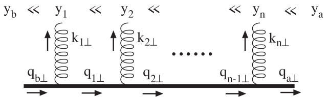
Figure 1: A BFKL ladder diagram. The heavy line represents the reggeized gluon exchanged in the $t$-channel.

We now consider the modified BFKL equation at LL, given by

$$f(y_{a}-y_{b},q_{a\perp},q_{b\perp}) = {1\over 2}\delta^{2}(q_{a\perp}-q_{b\perp})\Theta(y_{a}-y_{b}-\Delta)$$ (6)

$$+\ {\bar{\alpha}_{s}\over\pi}\int_{y_{b}+\Delta}^{y_{a}-\Delta}dy\int{d^{2}k_{\perp}\over k_{\perp}^{2}}\Biggl{[}f(y-y_{b},q_{a\perp}\!+\!k_{\perp},q_{b\perp})$$

$$\qquad\qquad\qquad-{q_{a\perp}^{2}\over k_{\perp}^{2}+(q_{a\perp}+k_{\perp})^{2}}f(y-y_{b},q_{a\perp},q_{b\perp})\Biggr{]}\ ,$$

where $\bar{\alpha}_{s}=\alpha_{s}N_{c}/\pi$. The function $f(y_{ab},q_{a\perp},q_{b\perp})$ is the BFKL Green’s function which describes the flow of transverse momentum from $q_{b\perp}$ to $q_{a\perp}$ by the emission of real and virtual gluons along the rapidity interval $y_{ab}=y_{a}-y_{b}$. The $\Delta$-dependence in this equation just enforces the constraint $y_{i+1}-y_{i}>\Delta$ for each successive emitted gluon in the ladder. To be consistent, the constraint is applied to the integrals in rapidity which are associated with both the real and virtual gluons. For $\Delta=0$ this equation just reduces to the standard BFKL equation, but eq. (6) gives an equally valid LL resummation for any $\Delta\ll y_{ab}$.

We can easily solve eq. (6) in the same manner as the original BFKL solution. First, perform a Mellin transform on this equation, defining

$$f_{\omega}(q_{a\perp},q_{b\perp})\ =\ \int_{\Delta}^{\infty}dy\,e^{-\omega(y-\Delta)}f(y,q_{a\perp},q_{b\perp}).$$ (7)

This gives the equation

$$\omega\,f_{\omega}(q_{a\perp},q_{b\perp})\ =\ {1\over 2}\delta^{2}(q_{a\perp}-q_{b\perp})$$ (8)

$$\qquad+\ e^{-\omega\Delta}\,{\bar{\alpha}_{s}\over\pi}\int{d^{2}k_{\perp}\over k_{\perp}^{2}}\Biggl{[}f_{\omega}(q_{a\perp}\!+\!k_{\perp},q_{b\perp})-{q_{a\perp}^{2}\over k_{\perp}^{2}+(q_{a\perp}+k_{\perp})^{2}}f_{\omega}(q_{a\perp},q_{b\perp})\Biggr{]}\ ,$$

The integral operator over the transverse momentum space has the same eigenfunctions and eigenvalues as the original BFKL equation, so we can immediately write down the solution to this equation:

$$f_{\omega}(q_{a\perp},q_{b\perp})\ =\ {1\over(2\pi)^{2}}\sum_{n=-\infty}^{\infty}e^{in\phi}\,\int_{-\infty}^{\infty}d\nu\,{(q_{a\perp}^{2})^{-1/2+i\nu}\,(q_{b\perp}^{2})^{-1/2-i\nu}\over\omega-\omega(n,\nu)\,e^{-\omega\Delta}}\ ,$$ (9)

where $\phi=\phi_{a}-\phi_{b}$ and the eigenvalue of the integral operator is

$$\omega(n,\nu)\ =\ 2\bar{\alpha}_{s}\left[\psi(1)-{\rm Re}\,\psi\left({|n|+1\over 2}+i\nu\right)\right]\ ,$$ (10)

where $\psi$ is the logarithmic derivative of the gamma function.

By performing the inverse Mellin transform, we obtain the BFKL Green’s function as a function of the rapidity interval $y$:

$$f(y,q_{a\perp},q_{b\perp})\ =\ {1\over(2\pi)^{2}}\sum_{n=-\infty}^{\infty}e^{in\phi}\,\int_{-\infty}^{\infty}d\nu\,{(q_{a\perp}^{2})^{-1/2+i\nu}\,(q_{b\perp}^{2})^{-1/2-i\nu}e^{\tilde{\omega}(n,\nu)(y-\Delta)}\over 1+\tilde{\omega}(n,\nu)\Delta}\ ,$$ (11)

where $\tilde{\omega}(n,\nu)$ is a solution of the equation [20, 21]

$$\tilde{\omega}(n,\nu)\ =\ \omega(n,\nu)e^{-\tilde{\omega}(n,\nu)\Delta}\ .$$ (12)

It is an interesting exercise to expand the equation (11) order-by-order as a power series in $\bar{\alpha}_{s}$. This is done using the formula:

$${e^{\tilde{\omega}(n,\nu)(y-\Delta)}\over 1+\tilde{\omega}(n,\nu)\Delta}\ =\ \sum_{m=0}{\omega(n,\nu)^{m}[y-(m+1)\Delta]^{m}\over m!}\ .$$ (13)

The factor $[y-(m+1)\Delta]^{m}/m!$ in (13) is exactly the phase space in rapidity for $m$ intermediate gluons, subject to the constraint $y_{i+1}-y_{i}>\Delta$. In fact, for a given rapidity interval $y$ the series should actually be truncated at the largest value of $m$ for which $[y-(m+1)\Delta]>0$, because one cannot put any more gluons in the rapidity interval and still obey the constraint. However, we also note that the power series converges only asymptotically to the analytic expression on the left-hand side of (13), and the best approximation is obtained by the truncated series. Thus, as $y/\Delta$ is increased, the analytic solution and the truncated series become arbitrarily close.

For asymptotically-large $y$ we can perform the integration over $\nu$ in eq. (11) using the saddle-point approximation. The eigenvalue $\tilde{\omega}(n,\nu)$ is largest for $n=0$ and is strongly peaked near $\nu=0$. Thus, we may keep only the first term in the Fourier series in $\phi$, and we can expand

$$\tilde{\omega}(0,\nu)\ =\ \tilde{A}-\tilde{B}\nu^{2}+\ \cdots\ .$$ (14)

The coefficients $\tilde{A}$ and $\tilde{B}$ are related to the standard BFKL saddle-point coefficients,

$$A\ =\ 4\bar{\alpha}_{s}\ln{2};\qquad\qquad B\ =\ 14\bar{\alpha}_{s}\zeta(3)\ ,$$ (15)

as solutions to the equations

$$\tilde{A} = Ae^{-\tilde{A}\Delta}$$

$$\tilde{B} = {B\,(\tilde{A}/A)\over 1+\tilde{A}\Delta}\ .$$ (16)

Evaluating the integral over $\nu$ in the saddle-point approximation gives

$$f(y,q_{a\perp},q_{b\perp})\ =\ {e^{\tilde{A}(y-\Delta)}\over 4\pi|q_{a\perp}||q_{b\perp}|\,(1+\tilde{A}\Delta)\,\sqrt{\tilde{B}\pi\tilde{y}}}\,\exp{\left(-{\ln^{2}(q_{a\perp}^{2}/q_{b\perp}^{2})\over 4\tilde{B}\tilde{y}}\right)}\ ,$$ (17)

where

$$\tilde{y}\ =\ y-\Delta{2+\tilde{A}\Delta\over 1+\tilde{A}\Delta}\ .$$ (18)

Using the relation $y=\ln(\hat{s}/|q_{a\perp}||q_{b\perp}|)$, we recognize that the quantity $\tilde{A}$ is related to the BFKL Pomeron intercept ($\tilde{A}=\omega_{P}-1$). For $\Delta\geq 0$ it is bounded by $0<\tilde{A}\leq A$. In table 1 we give the magnitude of $\tilde{A}$ for several representative values of the rapidity-separation parameter $\Delta$ with $\alpha_{s}=0.15$. For $\Delta=2$, the prediction for $\tilde{A}$ is reduced substantially, from 0.397 to 0.244. Recall that any of these predictions are equally valid in the LL approximation, assuming that $y\gg\Delta$.

$\phantom{\Biggl{[}}\Delta$	0	0.5	1	1.5	2
$\phantom{\Biggl{[}}\tilde{A}$	0.397	0.336	0.296	0.266	0.244

Table 1: BFKL Pomeron intercept $\tilde{A}=\omega_{P}-1$ at LL for several values of rapidity-separation parameter $\Delta$, with $\alpha_{s}=0.15$.

3 $\Delta$-dependent Gluon Anomalous Dimension

We can use eqs. (9) and (11) to obtain the gluon-gluon splitting function at small $x$ by introducing a $k_{\perp}$-dependent gluon distribution function ${\cal F}(x,k_{\perp})$, which is related to the standard gluon distribution function $g(x,M^{2})$ via

$$xg(x,M^{2})\ =\ \int d^{2}k_{\perp}{\cal F}(x,k_{\perp})\,\Theta(M^{2}-k_{\perp}^{2})\ ,$$ (19)

where $M$ is the factorization scale. The function ${\cal F}(x,k_{\perp})$ satisfies the inhomogeneous BFKL equation, so that it has a general solution of the form

$${\cal F}(x,k_{\perp})\ =\ \int_{x}^{1}{dz\over z}f(\ln{z/x},q_{\perp},k_{\perp})\,{\cal F}_{0}(z,q_{\perp})\bigg{|}_{q_{\perp}\rightarrow 0}\ ,$$ (20)

where ${\cal F}_{0}(z,q_{\perp})$ can be considered a “bare” gluon distribution and $q_{\perp}$ is used as an infrared cutoff. The splitting function can then be obtained by taking the derivative $\partial g(x,M^{2})/\partial\ln{M^{2}}$. In practice, it is more convenient to work with the moments of these equations to obtain the gluon-operator anomalous dimension, which is related to the gluon-gluon splitting function by

$$\gamma_{N}\ =\ {\alpha_{s}\over 2\pi}\int_{0}^{1}dx\,x^{N-1}P_{gg}(x)\ .$$ (21)

Following this line of argument, we obtain the anomalous dimension as the implicit solution to the equation [20]

$${\bar{\alpha}_{s}e^{-(N-1)\Delta}\over N-1}\left[2\psi(1)-\psi(\gamma_{N})-\psi(1-\gamma_{N})\right]\ =\ 1\ .$$ (22)

In order to interpret the $\Delta$-dependence of eq. (22), it is useful to solve it as a power series in $\bar{\alpha}_{s}$ and then transform back to $x$-space. The power series takes the form

$${\alpha_{s}\over 2\pi}P_{gg}(x)\ =\ {\bar{\alpha}_{s}\over x}\sum_{m=0}C_{m}{\bar{\alpha}_{s}^{m}\left[\ln{1/x}-(m+1)\Delta\right]^{m}\over m!}\ ,$$ (23)

where $C_{0}=1$, $C_{1}=C_{2}=0$, $C_{3}=2\zeta(3)$, etc. As in the last section we see that this expansion is an asymptotic series, which can be best approximated by truncating at the largest value of $m$ for which $[\ln{1/x}-(m+1)\Delta]>0$. The zeroth term in the expansion just corresponds to the standard double-logarithmic scaling of the DGLAP equation [25]. Thus, to see any effects of the resummation beyond double-logarithmic scaling, this expansion suggests that we must at the very least require

$$x\mathrel{\mathchoice{\lower 3.01385pt\vbox{\halign{$\matth\displaystyle\hfil#\hfil$\cr<\crcr\sim\crcr}}}{\lower 3.01385pt\vbox{\halign{$\matth\textstyle\hfil#\hfil$\cr<\crcr\sim\crcr}}}{\lower 3.01385pt\vbox{\halign{$\matth\scriptstyle\hfil#\hfil$\cr<\crcr\sim\crcr}}}{\lower 3.01385pt\vbox{\halign{$\matth\scriptscriptstyle\hfil#\hfil$\cr<\crcr\sim\crcr}}}}e^{-4\Delta}\ .$$ (24)

This requirement is fairly strong, because the first nonzero correction occurs at $\alpha_{s}^{3}$. For $\Delta=1$ and $\Delta=2$, this gives $x\mathrel{\mathchoice{\lower 3.01385pt\vbox{\halign{$\matth\displaystyle\hfil#\hfil$\cr<\crcr\sim\crcr}}}{\lower 3.01385pt\vbox{\halign{$\matth\textstyle\hfil#\hfil$\cr<\crcr\sim\crcr}}}{\lower 3.01385pt\vbox{\halign{$\matth\scriptstyle\hfil#\hfil$\cr<\crcr\sim\crcr}}}{\lower 3.01385pt\vbox{\halign{$\matth\scriptscriptstyle\hfil#\hfil$\cr<\crcr\sim\crcr}}}}2\times 10^{-2}$ and $x\mathrel{\mathchoice{\lower 3.01385pt\vbox{\halign{$\matth\displaystyle\hfil#\hfil$\cr<\crcr\sim\crcr}}}{\lower 3.01385pt\vbox{\halign{$\matth\textstyle\hfil#\hfil$\cr<\crcr\sim\crcr}}}{\lower 3.01385pt\vbox{\halign{$\matth\scriptstyle\hfil#\hfil$\cr<\crcr\sim\crcr}}}{\lower 3.01385pt\vbox{\halign{$\matth\scriptscriptstyle\hfil#\hfil$\cr<\crcr\sim\crcr}}}}3\times 10^{-4}$, respectively, before one would expect to see some deviation from double-logarithmic scaling at small $x$.

4 Modified BFKL Equation at NLL

As seen in the last two sections, the effects of the BFKL resummation can depend strongly on the rapidity-separation parameter $\Delta$, even though the dependence is formally NLL. Furthermore, we argued in the introduction that a nonzero value of $\Delta$ seems appropriate, although it is not obvious what is the best choice for this parameter. Thus, we need to consider how to perform a NLL calculation, while retaining the dependence on $\Delta$. In this section we show how to obtain the $\Delta$-dependence of the NLL kernel, and we explore its consequences.

The generalization of the $\Delta$-dependent BFKL equation takes the form

$$f(y_{a}-y_{b},q_{a\perp},q_{b\perp}) = {1\over 2}\delta^{2}(q_{a\perp}-q_{b\perp})\Theta(y_{a}-y_{b}-\Delta)$$ (25)

$$+\ \int_{y_{b}+\Delta}^{y_{a}-\Delta}dy\,K_{\Delta}\left[f(y-y_{b},q_{a\perp},q_{b\perp})\right]\ ,$$

where $K_{\Delta}$, which depends on $\Delta$, is an integral operator acting on the transverse momentum $q_{a\perp}$. This operator can be expanded as a power series in $\bar{\alpha}_{s}$:

$$K_{\Delta}\ =\ \bar{\alpha}_{s}K^{(1)}+\bar{\alpha}_{s}^{2}K^{(2)}+O(\bar{\alpha}_{s}^{3})\ ,$$ (26)

where the first term $K^{(1)}$, which gives the LL equation, is $\Delta$-independent. It can be read directly off of eq. (6), yielding

$$K^{(1)}\left[f(q_{\perp})\right]\ =\ {1\over\pi}\int{d^{2}\ell_{\perp}\over(\ell_{\perp}-q_{\perp})^{2}}\Biggl{[}f(\ell_{\perp})-{q_{\perp}^{2}\over\ell_{\perp}^{2}+(\ell_{\perp}-q_{\perp})^{2}}f(q_{\perp})\Biggr{]}$$ (27)

for any function $f(q_{\perp})$.

The second term $K^{(2)}$ in eq. (26) contains the NLL corrections to the BFKL kernel, and in the present formulation it will depend on the parameter $\Delta$. The $\Delta$-dependence of this term can be found by the requirement that the total dependence on $\Delta$ of the high energy cross section must vanish up to NNLL terms. That is, if we expand the hard cross section for scattering of partons $i$ and $j$,

$$\hat{\sigma}_{NLL}^{ij}\ =\ \int d^{2}q_{a\perp}d^{2}q_{b\perp}\,V^{i}(q_{a\perp})\,f(y_{a}-y_{b},q_{a\perp},q_{b\perp})\,V^{j}(q_{b\perp})\ ,$$ (28)

in powers of $\alpha_{s}$, the coefficients of all terms of the form $\alpha_{s}^{b+1}(\alpha_{s}y)^{n}$ should be independent of $\Delta$, where the Born term is $O(\alpha_{s}^{b})$. In this equation the quantities $V^{i}(q_{\perp})$ are the impact factors, which can also be expanded in a power series in $\bar{\alpha}_{s}$:

$$V^{i}(q_{\perp})\ =\ V^{i(0)}(q_{\perp})+\bar{\alpha}_{s}V^{i(1)}(q_{\perp})+O(\bar{\alpha}_{s}^{2})\ .$$ (29)

The condition for $\Delta$-independence of the cross section (28) to NLL is now obtained by inserting the iterated solution to (25) in (28), using (26) and (29), and requiring that the coefficients of the terms of the form $\alpha_{s}^{b+1}(\alpha_{s}y)^{n}$ are independent of $\Delta$. We find that the NLL kernel must be of the form

$$K^{(2)}\left[f(q_{\perp})\right]\ =\ K^{(2)}\left[f(q_{\perp})\right]\bigg{|}_{\Delta=0}+\Delta\,K^{(1)}\!\!\left[K^{(1)}\left[f(q_{\perp})\right]\right]\ ,$$ (30)

where the first term is the $\Delta$-independent BFKL kernel given in Ref. [4], and all of the $\Delta$-dependence is in the second term. Similarly, the NLL impact factors are of the form

$$V^{i(1)}(q_{\perp})\ =\ V^{i(1)}(q_{\perp})\bigg{|}_{\Delta=0}+\Delta\,K^{(1)}\!\!\left[V^{i(0)}(q_{\perp})\right]\ .$$ (31)

The virtual correction component of these results, (30) and (31), can also be obtained by considering the $\Delta$-dependent modification of the gluon-reggeization prescription, as discussed in the appendix.

At this stage we follow the lead of Ref. [4] and consider the action of the NLL kernel on the LL eigenfunctions, which have been modified so that the eigenvalue is symmetric in $\nu$. Specifically, we apply the operator (26) to the $n=0$ eigenfunction, which dominates at high-energy and gives the contribution to the total cross section. We find

$$K_{\Delta}\left[\alpha_{s}(q_{\perp}^{2})^{-1/2}\,(q_{\perp}^{2})^{-1/2+i\nu}\right]\ =\ \omega(\nu)\,\alpha_{s}(q_{\perp}^{2})^{-1/2}\,(q_{\perp}^{2})^{-1/2+i\nu}\$$ (32)

with

$$\omega(\nu)\ =\ \omega^{(0)}(\nu)\left(1-{\bar{\alpha}_{s}\over 4}\bar{c}(1/2+i\nu)\right)+\Delta\,\left(\omega^{(0)}(\nu)\right)^{2}\ .$$ (33)

In this equation $\omega^{(0)}(\nu)$ is the LL eigenvalue with running coupling:

$$\omega^{(0)}(\nu)\ =\ 2\bar{\alpha}_{s}(q_{\perp})\left[\psi(1)-{\rm Re}\,\psi\left({1\over 2}+i\nu\right)\right]\ ,$$ (34)

while the function $\bar{c}(\gamma)$ contains the $\Delta$-independent NLL corrections to the eigenfunction. The exact expression for $\bar{c}(\gamma)$ can be obtained from the function $c(\gamma)$ in Ref. [4] by removing the terms antisymmetric in $\nu$. The last term in (33) is the modification of the NLL eigenfunction due to the rapidity-separation constraint.

We now consider the solution of the modified BFKL equation at NLL. For simplicity we will ignore the effects of the running coupling. Then, following the same procedure as in section 2, one obtains the BFKL Green’s function solution (11) as an integral over $\nu$ with the coefficient of the rapidity in the exponent given by the implicit solution to

$$\tilde{\omega}(\nu)\ =\ \omega(\nu)e^{-\tilde{\omega}(\nu)\Delta}\ .$$ (35)

The saddle-point approximation to the integral (11) is determined in terms of the expansion of $\tilde{\omega}(\nu)$ around $\nu=0$:

$$\tilde{\omega}(\nu)\ =\ \tilde{A}-\tilde{B}\nu^{2}+\cdots\ ,$$ (36)

where the coefficients $\tilde{A}$ and $\tilde{B}$ are related to the equivalent coefficients $A$ and $B$ in the expansion of $\omega(\nu)$ by

$$\tilde{A} = Ae^{-\tilde{A}\Delta}$$

$$\tilde{B} = {B\,(\tilde{A}/A)\over 1+\tilde{A}\Delta}\ .$$ (37)

The values of $A$ and $B$ are

$$A\ =\ 2.77\bar{\alpha}_{s}+(-18.34+7.69\Delta)\bar{\alpha}_{s}^{2}$$ (38)

and

$$B\ =\ 16.83\bar{\alpha}_{s}+(-321.49+93.32\Delta)\bar{\alpha}_{s}^{2}$$ (39)

for three active flavors.

The coefficient $\tilde{A}$ is related to the BFKL Pomeron intercept by $\tilde{A}=\omega_{P}-1$. In figure 2 we plot both the LL and the NLL predictions for $\tilde{A}$ as a function of $\Delta$ for $\alpha_{s}=0.15$. We note that, although the NLL corrections to $\tilde{A}$ are large for $\Delta=0$, they are not large for $\Delta\mathrel{\mathchoice{\lower 3.01385pt\vbox{\halign{$\matth\displaystyle\hfil#\hfil$\cr>\crcr\sim\crcr}}}{\lower 3.01385pt\vbox{\halign{$\matth\textstyle\hfil#\hfil$\cr>\crcr\sim\crcr}}}{\lower 3.01385pt\vbox{\halign{$\matth\scriptstyle\hfil#\hfil$\cr>\crcr\sim\crcr}}}{\lower 3.01385pt\vbox{\halign{$\matth\scriptscriptstyle\hfil#\hfil$\cr>\crcr\sim\crcr}}}}2$ and they vanish for $\Delta=2.4$. Furthermore, the dependence of the NLL solution on $\Delta$ is very weak for $\Delta\mathrel{\mathchoice{\lower 3.01385pt\vbox{\halign{$\matth\displaystyle\hfil#\hfil$\cr>\crcr\sim\crcr}}}{\lower 3.01385pt\vbox{\halign{$\matth\textstyle\hfil#\hfil$\cr>\crcr\sim\crcr}}}{\lower 3.01385pt\vbox{\halign{$\matth\scriptstyle\hfil#\hfil$\cr>\crcr\sim\crcr}}}{\lower 3.01385pt\vbox{\halign{$\matth\scriptscriptstyle\hfil#\hfil$\cr>\crcr\sim\crcr}}}}2$.

Figure 2: BFKL Pomeron intercept $\tilde{A}=\omega_{P}-1$ at LL and NLL as a function of $\Delta$ for $\alpha_{s}=0.15$.

Figure 3: The coefficient $\tilde{B}$ of eq. (36) at LL and NLL as a function of $\Delta$ for $\alpha_{s}=0.15$.

In figure 3 we plot the coefficient $\tilde{B}$ at LL and NLL as a function of $\Delta$ for $\alpha_{s}=0.15$. At $\Delta=0$ it is negative indicating that the standard BFKL eigenvalue has a minimum at $\nu=0$ rather than a maximum [17]. It has been suggested that this leads to disastrous consequences such as oscillations in the cross section [18]. At the very least it shows that the interpretation of $\tilde{A}$ as the Pomeron intercept $\omega_{P}-1$ is invalid at $\Delta=0$. However, for $\Delta\mathrel{\mathchoice{\lower 3.01385pt\vbox{\halign{$\matth\displaystyle\hfil#\hfil$\cr>\crcr\sim\crcr}}}{\lower 3.01385pt\vbox{\halign{$\matth\textstyle\hfil#\hfil$\cr>\crcr\sim\crcr}}}{\lower 3.01385pt\vbox{\halign{$\matth\scriptstyle\hfil#\hfil$\cr>\crcr\sim\crcr}}}{\lower 3.01385pt\vbox{\halign{$\matth\scriptscriptstyle\hfil#\hfil$\cr>\crcr\sim\crcr}}}}2.2$ the coefficient $\tilde{B}$ becomes positive again, so the modified solution does have a maximum at $\nu=0$, and we can again identify $\tilde{A}$ with the BFKL Pomeron intercept. This suggests that a value of the rapidity-separation parameter of $\Delta\mathrel{\mathchoice{\lower 3.01385pt\vbox{\halign{$\matth\displaystyle\hfil#\hfil$\cr>\crcr\sim\crcr}}}{\lower 3.01385pt\vbox{\halign{$\matth\textstyle\hfil#\hfil$\cr>\crcr\sim\crcr}}}{\lower 3.01385pt\vbox{\halign{$\matth\scriptstyle\hfil#\hfil$\cr>\crcr\sim\crcr}}}{\lower 3.01385pt\vbox{\halign{$\matth\scriptscriptstyle\hfil#\hfil$\cr>\crcr\sim\crcr}}}}2.2$ is more natural than the standard choice of $\Delta=0$. On this basis, we estimate the value of the NLL BFKL Pomeron intercept to be between 0.22 and 0.25 for $\alpha_{s}=0.15$.

5 Conclusions

In this paper we have considered the modification of the BFKL resummation by requiring that the rapidities of successively emitted gluons must satisfy the constraint $y_{i+1}-y_{i}>\Delta$. The inclusion of an arbitrary “renormalization” constant, such as $\Delta$, in the BFKL resummation is a natural thing to do, because in such a resummation of large logarithms one can always redefine the energy scale in the logarithm. The particular implementation of this arbitrary constant (the “renormalization scheme”) as a constraint on the rapidity separations is nice because it has an obvious physical interpretation. Using this interpretation, we have argued and we have seen through specific calculations that the choice of $\Delta=0$ is not the best choice for performing the resummation. This is analogous to performing a fixed-order calculation using an inappropriate choice of the ultraviolet renormalization scale $\mu$. The next-to-leading corrections are large, not because the perturbative calculation is inherently bad, but because one has simply made a poor choice of scale.

We have shown how to consistently include the rapidity-separation constraint, both at LL and at NLL. At LL we find that the prediction for the BFKL Pomeron intercept decreases monotonically as $\Delta$ increases, while at NLL it increases rapidly from $\Delta=0$ and then becomes quite insensitive to $\Delta$ for $\Delta\mathrel{\mathchoice{\lower 3.01385pt\vbox{\halign{$\matth\displaystyle\hfil#\hfil$\cr>\crcr\sim\crcr}}}{\lower 3.01385pt\vbox{\halign{$\matth\textstyle\hfil#\hfil$\cr>\crcr\sim\crcr}}}{\lower 3.01385pt\vbox{\halign{$\matth\scriptstyle\hfil#\hfil$\cr>\crcr\sim\crcr}}}{\lower 3.01385pt\vbox{\halign{$\matth\scriptscriptstyle\hfil#\hfil$\cr>\crcr\sim\crcr}}}}2$ and $\alpha_{s}=0.15$. Furthermore, the NLL corrections are relatively small compared to the LL prediction for $\Delta\mathrel{\mathchoice{\lower 3.01385pt\vbox{\halign{$\matth\displaystyle\hfil#\hfil$\cr>\crcr\sim\crcr}}}{\lower 3.01385pt\vbox{\halign{$\matth\textstyle\hfil#\hfil$\cr>\crcr\sim\crcr}}}{\lower 3.01385pt\vbox{\halign{$\matth\scriptstyle\hfil#\hfil$\cr>\crcr\sim\crcr}}}{\lower 3.01385pt\vbox{\halign{$\matth\scriptscriptstyle\hfil#\hfil$\cr>\crcr\sim\crcr}}}}2$. We have also seen that the eigenvalue has a maximum at $\nu=0$ as long as $\Delta\mathrel{\mathchoice{\lower 3.01385pt\vbox{\halign{$\matth\displaystyle\hfil#\hfil$\cr>\crcr\sim\crcr}}}{\lower 3.01385pt\vbox{\halign{$\matth\textstyle\hfil#\hfil$\cr>\crcr\sim\crcr}}}{\lower 3.01385pt\vbox{\halign{$\matth\scriptstyle\hfil#\hfil$\cr>\crcr\sim\crcr}}}{\lower 3.01385pt\vbox{\halign{$\matth\scriptscriptstyle\hfil#\hfil$\cr>\crcr\sim\crcr}}}}2.2$, so that the bad behavior seen in the saddle-point approximation is no longer a problem. It is interesting to note that our results for large $\Delta$ are in reasonable agreement with the results of Ref. [28], which addresses the question of the large NLL corrections by resumming double logarithms in transverse momenta. Presumably, the same sort of correlation effects are being included by the two very different approaches.

In conclusion, we believe that for a reasonable range of the rapidity-separation parameter $\Delta$ the modified BFKL formalism is a theoretically consistent and stable resummation of the perturbation series in $\alpha_{s}$ at high-enough energies. However, the phenomenological usefulness of this resummation is still an open question. If we assume that $\Delta>2$ is required to consistently use the modified-BFKL resummation, then one should not expect to see significant deviations from double-logarithmic scaling at small-$x$ in the gluon-gluon splitting functions at least until $x\mathrel{\mathchoice{\lower 3.01385pt\vbox{\halign{$\matth\displaystyle\hfil#\hfil$\cr<\crcr\sim\crcr}}}{\lower 3.01385pt\vbox{\halign{$\matth\textstyle\hfil#\hfil$\cr<\crcr\sim\crcr}}}{\lower 3.01385pt\vbox{\halign{$\matth\scriptstyle\hfil#\hfil$\cr<\crcr\sim\crcr}}}{\lower 3.01385pt\vbox{\halign{$\matth\scriptscriptstyle\hfil#\hfil$\cr<\crcr\sim\crcr}}}}3\times 10^{-4}$. Similarly, equation (13) suggests that in large-rapidity dijet production one needs rapidity intervals of $y\mathrel{\mathchoice{\lower 3.01385pt\vbox{\halign{$\matth\displaystyle\hfil#\hfil$\cr>\crcr\sim\crcr}}}{\lower 3.01385pt\vbox{\halign{$\matth\textstyle\hfil#\hfil$\cr>\crcr\sim\crcr}}}{\lower 3.01385pt\vbox{\halign{$\matth\scriptstyle\hfil#\hfil$\cr>\crcr\sim\crcr}}}{\lower 3.01385pt\vbox{\halign{$\matth\scriptscriptstyle\hfil#\hfil$\cr>\crcr\sim\crcr}}}}4$ before the BFKL formalism would begin to be applicable. Certainly, more detailed phenomenological study, using the insights gained from the NLL corrections, is needed in order to assess the importance of BFKL to experiment.

Acknowledgments We would like to thank Vittorio Del Duca and Wu-Ki Tung for useful comments on this manuscript.

Appendix A Modification of the Reggeized Gluons

An important requirement of our analysis is that the modification of the real and virtual gluon rapidity phase space is handled identically, so that the cancellation of the soft singularities remains intact. However, it is still possible to include the virtual corrections using a reggeized gluon, although with a slightly more complicated, $\Delta$-dependent form. For the modified BFKL equation (25) we find that the appropriate prescription for reggeizing a gluon of off-shellness $t_{i}$ is to replace the gluon propagator by

$${1\over t_{i}}\rightarrow{1\over t_{i}}\,{e^{-\tilde{\lambda}(t_{i})\Delta/2}\over\sqrt{1+\tilde{\lambda}(t_{i})\Delta}}\,\left({s_{i+1,i}\over|k_{i+1\perp}||k_{i\perp}|}\right)^{\tilde{\lambda}(t_{i})/2}\ =\ {1\over t_{i}}\,{e^{\tilde{\lambda}(t_{i})(y_{i+1,i}-\Delta)/2}\over\sqrt{1+\tilde{\lambda}(t_{i})\Delta}}\,$$ (40)

where $\tilde{\lambda}(t)$ is related to the usual BFKL Regge intercept $\alpha(t)\equiv\lambda(t)/2$ by solving the equation

$$\tilde{\lambda}(t)\ =\ \lambda(t)e^{-\tilde{\lambda}(t)\Delta}\ .$$ (41)

Note that the square root in the equation (40) occurs because the rapidity phase space modification is defined at the squared-amplitude level, whereas the reggeization is defined at the amplitude level.

The quantity $\lambda(t)$ is just the purely virtual contribution to the kernel $K_{\Delta}$. It can be expanded as a power series in $\bar{\alpha}_{s}$:

$$\lambda(t)\ =\ \bar{\alpha}_{s}\lambda^{(1)}(t)+\bar{\alpha}_{s}^{2}\lambda^{(2)}(t)+O(\bar{\alpha}_{s}^{3})\ ,$$ (42)

where the $\Delta$-dependence begins with the $\lambda^{(2)}(t)$ term. At LL the kernel can be separated into a real and a virtual contribution:

$$K^{(1)}\left[f(q_{\perp})\right]\ =\ K^{(1)}_{r}\left[f(q_{\perp})\right]+K^{(1)}_{v}\left[f(q_{\perp})\right]\ ,$$ (43)

where

$$K^{(1)}_{v}\left[f(q_{\perp})\right]\ =\ \lambda^{(1)}(-q_{\perp}^{2})\,f(q_{\perp})\ ,$$ (44)

and $t=q^{2}\simeq-q_{\perp}^{2}$. Thus, $\lambda^{(1)}$ can be obtained directly from (27):

$$\lambda^{(1)}(-q_{\perp}^{2}) = -{1\over\pi(2\pi)^{-2\epsilon}}\int d^{2-2\epsilon}\ell_{\perp}\,{q_{\perp}^{2}\over(\ell_{\perp}-q_{\perp})^{2}\left(\ell_{\perp}^{2}+(\ell_{\perp}-q_{\perp})^{2}\right)}$$

$$= -{1\over(2\pi)^{1-2\epsilon}}\int d^{2-2\epsilon}\ell_{\perp}\,{q_{\perp}^{2}\over\ell_{\perp}^{2}(\ell_{\perp}-q_{\perp})^{2}}$$

$$= {1\over\epsilon}\left(\mu^{2}\over q_{\perp}^{2}\right)^{\epsilon}{\Gamma(1+\epsilon)\,\Gamma^{2}(1-\epsilon)\over(4\pi)^{-2\epsilon}\,\Gamma(1-2\epsilon)}\ .$$

We also obtain

$$K^{(1)}_{r}\left[f(q_{\perp})\right]\ =\ {1\over\pi(2\pi)^{-2\epsilon}}\int d^{2-2\epsilon}\ell_{\perp}\,{f(\ell_{\perp})\over(\ell_{\perp}-q_{\perp})^{2}}\ .$$ (46)

For definiteness we have used dimensional regularization with $d=4-2\epsilon$ dimensions to render the integrals finite.

At NLL the kernel can be separated into the real and virtual corrections to the Lipatov vertex $K^{(1)}_{r}$ plus the two-loop virtual contribution:

$$K^{(2)}\left[f(q_{\perp})\right]\ =\ K^{(2)}_{rr}\left[f(q_{\perp})\right]+K^{(2)}_{rv}\left[f(q_{\perp})\right]+K^{(2)}_{vv}\left[f(q_{\perp})\right]\ ,$$ (47)

where

$$K^{(2)}_{vv}\left[f(q_{\perp})\right]\ =\ \lambda^{(2)}(-q_{\perp}^{2})\,f(q_{\perp})\ .$$ (48)

Similarly, the NLL impact factors can be separated into real and virtual corrections:

$$V^{i(1)}(q_{\perp})\ =\ V^{i(1)}_{r}(q_{\perp})+V^{i(1)}_{v}(q_{\perp})\ .$$ (49)

It is now straightforward to verify the $\Delta$-dependence of the NLL kernel and impact factors given in equations (30) and (31), at least for the virtual components $K^{(2)}_{vv}$, $K^{(2)}_{rv}$, and $V^{i(1)}_{v}$. This is most easily seen by reorganizing the reggeized-gluon propagator (40) using

$${e^{\tilde{\lambda}(t)(y-\Delta)}\over{1+\tilde{\lambda}(t)\Delta}} = \left[1-2\bar{\alpha}_{s}\Delta\lambda^{(1)}(t)\right]\exp\left\{\left[\bar{\alpha}_{s}\lambda^{(1)}(t)+\bar{\alpha}_{s}^{2}[\lambda^{(2)}(t)-\Delta(\lambda^{(1)}(t))^{2}]\right]y\right\}$$ (50)

$$+\ {\cal O}\left(\bar{\alpha}_{s}^{2}[\bar{\alpha}_{s}y]^{n}\right)\ ,$$

where the remaining terms are effectively NNLL. Demanding $\Delta$-independence up to NNLL, one immediately obtains from the term in the exponent

$$\lambda^{(2)}(t)\ =\ \lambda^{(2)}(t)\bigg{|}_{\Delta=0}+\Delta\,\left(\lambda^{(1)}(t)\right)^{2}\ .$$ (51)

Using the modified form of the reggeized gluon in a $2\rightarrow n$ partons high-energy amplitude and expanding to one-loop order, as done in Refs. [12, 14], one also directly obtains

$$V^{i(1)}_{v}(q_{\perp})\ =\ V^{i(1)}_{v}(q_{\perp})\bigg{|}_{\Delta=0}+\Delta\,\lambda^{(1)}(-q_{\perp})\,V^{i(0)}(q_{\perp})\ ,$$ (52)

and

$$K^{(2)}_{rv}\left[f(q_{\perp})\right] = K^{(2)}_{rv}\left[f(q_{\perp})\right]\bigg{|}_{\Delta=0}$$ (53)

$$+\,\Delta\left(K^{(1)}_{r}\left[\lambda^{(1)}(-q_{\perp}^{2})f(q_{\perp})\right]+\lambda^{(1)}(-q_{\perp}^{2})\,K^{(1)}_{r}\left[f(q_{\perp})\right]\right)\ .$$

The equations (51), (52), and (53) are just the virtual-correction components of equations (30) and (31).

References

• [1] E.A. Kuraev, L.N. Lipatov and V.S. Fadin, Zh. Eksp. Teor. Fiz. 71, 840 (1976) [Sov. Phys. JETP 44, 443 (1976)].
• [2] E.A. Kuraev, L.N. Lipatov and V.S. Fadin, Zh. Eksp. Teor. Fiz. 72, 377 (1977) [Sov. Phys. JETP 45, 199 (1977)].
• [3] Ya.Ya. Balitsky and L.N. Lipatov, Yad. Fiz. 28 1597 (1978) [Sov. J. Nucl. Phys. 28, 822 (1978)].
• [4] V.S. Fadin and L.N. Lipatov, Phys. Lett. B429, 127 (1998).
• [5] V.S. Fadin, preprint hep-ph/9807528.
• [6] V.S. Fadin and L.N. Lipatov, Yad. Fiz. 50, 1141 (1989) [Sov. J. Nucl. Phys. 50, 712 (1989)]; Nucl. Phys. B477, 767 (1996).
• [7] V.S. Fadin and L.N. Lipatov, Nucl. Phys. B406, 259 (1993).
• [8] V.S. Fadin, R. Fiore and A. Quartarolo, Phys. Rev. D50 5893 (1994).
• [9] V.S. Fadin, R. Fiore and M.I. Kotsky, Phys. Lett. B389, 737 (1996).
• [10] V.S. Fadin, R. Fiore and M.I. Kotsky, Phys. Lett. B359, 181 (1995); B387 593 (1996);
V.S. Fadin, R. Fiore and A. Quartarolo, Phys. Rev. D53, 2729 (1996);
J. Blümlein, V. Ravindran, W.L. van Neerven, Phys. Rev. D58, 09152 (1998).
• [11] V. Del Duca, Phys. Rev. D54, 989, 4474 (1996).
• [12] V. Del Duca and C.R. Schmidt, Phys. Rev. D57, 4069 (1998).
• [13] V.S. Fadin and R. Fiore, Phys. Lett. B294, 286 (1992);
V.S. Fadin, R. Fiore and A. Quartarolo, Phys. Rev. D50, 2265 (1994).
• [14] V. Del Duca and C.R. Schmidt, preprint EDINBURGH 98/21, MSUHEP-80928, hep-ph/9810215.
• [15] Z. Bern, V. Del Duca and C.R. Schmidt, preprint EDINBURGH 98/20, MSUHEP-81016, UCLA/98/TEP/29, hep-ph/9810409.
• [16] G. Camici and M. Ciafaloni, Phys. Lett. B412, 396 (1997); Erratum-ibid. B417 390 (1998); Phys. Lett. B430, 349 (1998).
• [17] D.A. Ross, Phys. Lett. B431, 161 (1998).
• [18] E. Levin, preprint TAUP 2501-98, hep-ph/9806228.
• [19] R.D. Ball and S. Forte, preprint hep-ph/9805315;
J. Blümlein et al, Phys. Rev. D58, 014020 (1998); preprint hep-ph/9806368.
• [20] B. Andersson, G. Gustafson, J. Samuelsson, Nucl. Phys. B467, 443 (1996).
• [21] L.N. Lipatov, talk presented at the $4^{\rm th}$ Workshop on Small-$x$ and Diffractive Physics, Fermi National Accelerator Laboratory, Sept. 17-20, 1998.
• [22] C.R. Schmidt, Phys. Rev. Lett. 78, 4531 (1997).
• [23] L.H. Orr and W.J. Stirling, Phys. Rev. D56, 5875 (1997).
• [24] S. Catani and F. Hautmann, Nucl. Phys. B427, 475 (1994).
• [25] Y.L. Dokshitzer, Sov. Phys. JETP 73, 1216 (1977);
V.N. Gribov and L.N. Lipatov, Sov. J. Nucl. Phys. 15, 78 (1972);
G. Altarelli and G. Parisi, Nucl. Phys. B126, 298 (1977).
• [26] Y.V. Kovchegov and A.H. Mueller, Phys. Lett. B439, 428 (1998).
• [27] N. Armesto, J. Bartels, M.A. Braun, Phys. Lett. B442, 459 (1998).
• [28] G.P. Salam, J.High Energy Phys. 9807, 019 (1998).
• [29] A.H. Mueller and H. Navelet, Nucl. Phys. B282, 727 (1987).