Baryon masses in large $N_{c}$ chiral perturbation theory

Abstract

We analyse the baryon mass spectrum in a framework which combines the $1/N_{c}$ expansion with chiral perturbation theory. Meson loop contributions involving the full SU(3) octet of pseudoscalar Goldstone bosons are evaluated, and the influence of explicit chiral and flavor symmetry breaking by non-zero and unequal quark masses is investigated. We also discuss sigma terms and the strangeness contribution to the nucleon mass.

I Introduction

The large $N_{c}$ limit, where $N_{c}$ is the number of colors, is a useful device to understand many systematic features of baryon properties [1, 2], such as the $1/N_{c}$ scaling of various physical quantities. In a series of papers, Dashen and Manohar [3, 4], and Jenkins [5] have discussed the $1/N_{c}$ structure of baryon properties, and the framework for combining chiral symmetry with the large $N_{c}$ aspects of QCD has been developed by many authors [6, 7, 8, 9, 10, 11, 12]. In Refs. [7, 10], the baryon octet and decuplet mass spectra were discussed in this framework and the baryon mass relations were derived. However, although those works successfully reproduce mass relations at tree level, they do not compute all possible terms allowed by the chiral and large $N_{c}$ expansions.

The baryon mass spectrum was re-examined in conventional baryon chiral perturbation theory by Borasoy and Meissner [13, 14]. To compute the baryon masses to order $m_{q}^{2}$, where $m_{q}$ is the quark mass, the decuplet degrees of freedom are integrated out to give counter terms, and some low-energy constants are determined from resonance saturation. However, when we work with the $1/N_{c}$ expansion, the octet and decuplet states are degenerate at the leading order, and the decuplet fields must be treated explicitly.

In this paper, we re-examine the baryon masses in chiral perturbation theory taking into account the $1/N_{c}$ counting based on the techniques developed in the literature, e.g., in Refs. [9, 10, 11]. This enables us to investigate the $1/N_{c}$ structure of the baryon properties and the meson-baryon interactions in a systematic way. The baryon axial current matrix elements and the strangeness contribution to the nucleon mass are computed as well. Some of these topics were discussed in the literature [7, 10, 11] focusing on the leading order terms in $1/N_{c}$ expansion (up to one loop corrections). In this paper, we perform the calculations to the next orders and discuss a difficulty which arises in computing the one loop corrections in a way which is consistent with the $1/N_{c}$ expansion. This paper is organized as follows. In the next Section, we briefly discuss the formalism of this approach. In Section III, we compute the baryon axial current up to one-loop corrections. The baryon mass formulas are given in Section IV. The one-loop corrections to the baryon masses are calculated in Section V. We discuss the strangeness contribution to the nucleon mass and the sigma term in Section VI and then finish with a summary and conclusion in Section VII. Explicit expressions of baryon wave functions and some detailed formulas are given in Appendices.

II Formalism

We start with a brief review of the construction of baryon states in the large $N_{c}$ limit, referring to Refs.[9, 10, 15] for further details. The baryon states with $N_{c}$ quarks can be written as follows:

$$|B\rangle\equiv{\cal B}^{a_{1}\alpha_{1}\dots a_{N_{c}}\alpha_{N_{c}}}\varepsilon^{A_{1}\dots A_{N_{c}}}q^{\dagger}_{a_{1}\alpha_{1}A_{1}}\dots q^{\dagger}_{a_{N_{c}}\alpha_{N_{c}}A_{N_{c}}}|0),$$ (1)

in particle number space, where $a_{i}$ are the flavor indices, $\alpha_{i}$ the spin indices and $A_{i}$ the color indices. The quark creation and annihilation operators $q^{\dagger}$ and $q$ satisfy the usual anti-commutator relations for fermions. The symmetric tensor ${\cal B}$ is characteristic of each given baryon wave function. Since the baryons are in color-singlet states, however, it is more convenient to work with

$$|B)\equiv{\cal B}^{a_{1}\alpha_{1}\dots a_{N_{c}}\alpha_{N_{c}}}\alpha^{\dagger}_{a_{1}\alpha_{1}}\dots\alpha^{\dagger}_{a_{N_{c}}\alpha_{N_{c}}}|0),$$ (2)

by dropping the explicit color indices, where the operators $\alpha^{\dagger}$ and $\alpha$ are bosonic operators satisfying the usual commutator relations. For short-hand notation, we label the quark operators as

$$\alpha_{1}\equiv\alpha_{u\uparrow},\qquad\alpha_{2}\equiv\alpha_{u\downarrow},\qquad\alpha_{3}\equiv\alpha_{d\uparrow},$$ (3)

$$\alpha_{4}\equiv\alpha_{d\downarrow},\qquad\alpha_{5}\equiv\alpha_{s\uparrow},\qquad\alpha_{6}\equiv\alpha_{s\downarrow},$$ (4)

so that $\alpha_{1}^{\dagger}$ creates $u$-quark with spin-up, and so forth.

There is an ambiguity when we extrapolate the physical baryon states to large $N_{c}$. As in the literature, we keep the spin, isospin and strangeness of baryons as $O(1)$ in the large $N_{c}$ limit. For example, the nucleon state in large $N_{c}$ limit has spin 1/2, isospin 1/2 and no strangeness. This can be done by acting with spin-flavor singlet operators on the physical baryon states. For example, the proton spin-up state can be written as

$$|p,+{\textstyle\frac{1}{2}})=C_{N}\alpha_{1}^{\dagger}(A_{s}^{\dagger})^{n}|0),$$ (5)

where $n=(N_{c}-1)/2$ and $C_{N}$ is the normalization constant. The spin-isospin singlet operator $A_{s}^{\dagger}$ is defined as

$$A_{s}^{\dagger}=\alpha_{1}^{\dagger}\alpha_{4}^{\dagger}-\alpha_{2}^{\dagger}\alpha_{3}^{\dagger}.$$ (6)

One can easily verify that this state reduces to the usual quark model state in the real world with $N_{c}=3$. The complete list of the baryon octet and decuplet states can be found in Appendix A.

Next we define a one-body operator $\{X\}$ in spin-flavor space as

$$\{X\}=\alpha_{a\alpha}^{\dagger}X_{ab}^{\alpha\beta}\alpha_{b\beta},$$ (7)

so that its expectation value on baryon states is at most of $O(N_{c})$. In a similar way, one can define 2-body operators $\{X\}\{Y\}$ and 3-body operators $\{X\}\{Y\}\{Z\}$, and so on. Then, it is found that the coefficient of an $r$-body operator is at most $O(1/N_{c}^{r-\ell-1})$, where $\ell$ is the number of inner quark loops [9, 16]. This enables us to treat the coupling constants as $O(1)$ quantities in the large $N_{c}$ expansion by writing the $N_{c}$-dependence of the operators explicitly.

By direct evaluation, one can see the well-known commutator relation,

$$[\{X\},\{Y\}]=\{[X,Y]\}.$$ (8)

Note that the left-hand side is naively a two body operator whose expectation values can be of $O(N_{c}^{2})$, whereas the right-hand side is a one-body operator whose expectation values are of $O(N_{c})$ at most. This means that the order of an operator in $1/N_{c}$ counting reduces when we have a commutator structure as in Eq. (8). This plays an important role in the large $N_{c}$ analyses of the baryon properties.

We will discuss the explicit forms of some operators which appear in the calculation of baryon axial currents and masses in the next Sections.

III Baryon axial currents

A Tree level

Our starting point is the chiral meson-baryon effective Lagrangian. Baryon matrix elements of this Lagrangian involve the meson-baryon interaction in the following form:

$$\langle{\cal L}_{\rm eff}\rangle = g\,(B|\{A^{\mu}\sigma_{\mu}\}|B)+\frac{h}{N_{c}}\,(B|\{A^{\mu}\}\{\sigma_{\mu}\}|B)+\dots,$$ (9)

where $\sigma^{\mu}$ is the baryon spin matrix, and the dots denote higher order terms. The axial field $A_{\mu}$ is defined as

$$A_{\mu} = \frac{i}{2}(\xi\partial_{\mu}\xi^{\dagger}-\xi^{\dagger}\partial_{\mu}\xi),$$ (10)

where $\xi=\exp(i\Pi/f)$ with the meson decay constant $f$. The SU(3) matrix field $\Pi$ represents the octet of pseudoscalar Goldstone bosons. It is defined as

$$\Pi=\frac{1}{2}\lambda_{a}\pi_{a},$$ (11)

with the usual Gell-Mann matrices $\lambda_{a}$ $(a=1,\dots,8)$. In Eq. (9), the $N_{c}$ factors of operators are given explicitly, and the coupling constants $g$ and $h$ are of $O(1)$ in the $1/N_{c}$ counting.

Then the baryon axial current $J_{5,\mu}^{a}$ reads

$$J_{5,\mu}^{a}=\frac{g}{2}\,\{\tilde{T}^{a}\sigma_{\mu}\}+\frac{h}{2N_{c}}\,\{\tilde{T}^{a}\}\{\sigma_{\mu}\},$$ (12)

from the Lagrangian (9) with

$$\tilde{T}^{a}=\frac{1}{2}(\xi\lambda^{a}\xi^{\dagger}+\xi^{\dagger}\lambda^{a}\xi).$$ (13)

This gives its matrix elements as

$$(B^{\prime}|J_{5,\mu}^{a}|B)=\alpha_{B^{\prime}B}^{a}\bar{u}_{B^{\prime}}(\sigma_{\mu})u_{B}.$$ (14)

where $u_{B}$ is the Dirac spinor of the baryon and

$$\alpha_{B^{\prime}B}^{a}=g(B^{\prime}|\{{\textstyle\frac{1}{2}}\lambda^{a}\sigma^{3}\}|B)+\frac{h}{N_{c}}(B^{\prime}|\{{\textstyle\frac{1}{2}}\lambda^{a}\}\{\sigma^{3}\}|B),$$ (15)

at the tree level.

By using the wave functions given in Appendix A, we can compute the baryon axial current straightforwardly. A naive investigation of each term gives that, despite the $1/N_{c}$ factor, the $h$ term contribution is expected to be of the same order as that coming from the $g$ term. This is because the $h$ term contains a 2-body operator whose expectation value can be $O(N_{c}^{2})$, thus the leading order of the $h$ term contribution can be of $N_{c}$. However, close inspection shows that the $g$ term contribution dominates, because the $h$ term contains the operator $\{\sigma_{\mu}\}$ and our baryon wave functions satisfy $\{\sigma_{\mu}\}\sim O(1)$.

The explicit forms of the relevant operators are

$$\{{\textstyle\frac{1}{2}}\lambda^{1+i2}\sigma^{3}\}=\alpha_{1}^{\dagger}\alpha_{3}-\alpha_{2}^{\dagger}\alpha_{4}, \{{\textstyle\frac{1}{2}}\lambda^{4+i5}\sigma^{3}\}=\alpha_{1}^{\dagger}\alpha_{5}-\alpha_{2}^{\dagger}\alpha_{6},$$ (16)

$$\{{\textstyle\frac{1}{2}}\lambda^{1+i2}\}\{\sigma^{3}\}=\alpha_{1}^{\dagger}\alpha_{3}+\alpha_{2}^{\dagger}\alpha_{4}, \{{\textstyle\frac{1}{2}}\lambda^{4+i5}\}\{\sigma^{3}\}=\alpha_{1}^{\dagger}\alpha_{5}+\alpha_{2}^{\dagger}\alpha_{6},$$ (17)

so that we obtain

$$\alpha_{pn}^{1+i2} = \frac{g}{3}(N_{c}+2)+\frac{h}{N_{c}},$$ (18)

$$\alpha_{\Lambda\Sigma^{-}}^{1+i2} = \alpha_{\Sigma^{+}\Lambda}^{1+i2}=\frac{g}{3\sqrt{2}}\sqrt{(N_{c}-1)(N_{c}+3)},$$ (19)

$$\alpha_{\Xi^{0}\Xi^{-}}^{1+i2} = \frac{N_{c}g}{9}-\frac{h}{N_{c}},$$ (20)

$$\alpha_{\Sigma^{0}\Sigma^{-}}^{1+i2} = -\alpha_{\Sigma^{+}\Sigma^{0}}^{1+i2}=\frac{g}{3\sqrt{2}}(N_{c}+1)+\frac{\sqrt{2}h}{N_{c}},$$ (21)

and

$$\alpha_{p\Lambda}^{4+i5} = -\frac{g}{2}\sqrt{N_{c}+3}-\frac{h}{2N_{c}}\sqrt{N_{c}+3},$$ (22)

$$\alpha_{\Lambda\Xi^{-}}^{4+i5} = \frac{\sqrt{N_{c}}g}{2\sqrt{3}}+\frac{\sqrt{3}h}{2N_{c}}\sqrt{N_{c}-1},$$ (23)

$$\alpha_{p\Sigma^{0}}^{4+i5} = \frac{1}{\sqrt{2}}\alpha_{n\Sigma^{-}}^{4+i5}=\frac{g}{6}\sqrt{N_{c}-1}-\frac{h}{2N_{c}}\sqrt{N_{c}-1},$$ (24)

$$\alpha_{\Sigma^{0}\Xi^{-}}^{4+i5} = \frac{1}{\sqrt{2}}\alpha_{\Sigma^{+}\Xi^{0}}^{4+i5}=\frac{5g}{6\sqrt{3}}\sqrt{N_{c}+3}+\frac{h}{2\sqrt{3}N_{c}}\sqrt{N_{c}+3}.$$ (25)

These results show that the $h$ term contributions are suppressed as compared to those of the $g$ terms as we discussed above. We can also find that the leading order of $\alpha^{1+i2}_{BB^{\prime}}$ is $O(N_{c})$, whereas $\alpha^{4+i5}_{BB^{\prime}}$, which changes the baryon strangeness, is $O(\sqrt{N_{c}})$. This shows that the strangeness-changing (i.e., $\Delta S\neq 0$) baryon axial currents are suppressed as compared to the strangeness-conserving (i.e., $\Delta S=0$) baryon axial currents by $O(\sqrt{N_{c}})$. This can be understood from Eq. (17) by noting that the number of $u$,$d$ quarks in the baryon wave functions is $O(N_{c})$ whereas that of $s$ quark, i.e., strangeness, is $O(N_{c}^{0})$. For example, in the case of $\alpha_{pn}^{1+i2}$, acting with $\alpha_{3}$ (or $\alpha_{4}$) on the baryon state gives the factor $N_{c}$, and the inner product of initial and final baryon wave functions with the proper normalization constants gives $O(1)$, so that $\alpha_{pn}^{1+i2}$ is $O(N_{c})$. However, for $\alpha_{p\Lambda}^{4+i5}$, the action with $\alpha_{5}$ (or $\alpha_{6}$) gives $O(N_{c}^{0})$ because our baryon wave functions have the strangeness of $O(N_{c}^{0})$. Since the normalization constants of nucleon and $\Lambda$ are $O(1/N_{c})$ and $O(1/\sqrt{N_{c}})$, respectively, we have an additional factor $\sqrt{N_{c}}$ in the calculation of $\alpha_{p\Lambda}^{4+i5}$, which implies that the order of $\alpha_{p\Lambda}^{4+i5}$ is $O(\sqrt{N_{c}})$.

Since the contributions of the $h$ term are suppressed as compared to those of the $g$ term by $O(1/N_{c}^{2})$ for the $\Delta S=0$ axial currents and by $O(1/N_{c})$ for the $\Delta S=1$ axial currents, we can neglect the $h$ term up to next to leading order. At this order, when we fix $N_{c}=3$, we can recover the quark model relation [10],

$$D=g,\qquad F=\frac{2}{3}g,$$ (26)

by comparing with the results of the baryon chiral perturbation theory [17, 18] in addition to the quark model predictions

$${\cal C}=-2g,\qquad{\cal H}=-3g,$$ (27)

for the octet-decuplet-meson and decuplet-decuplet-meson coupling constants, ${\cal C}$ and ${\cal H}$, defined as in Ref. [19]. When we go further in the $1/N_{c}$ expansion, we must include the $h$ term, and we get the modified relations,

$$D=g,\qquad F=\frac{2g+h}{3},$$ (28)

as found in Ref. [10].

We also compute $\alpha_{B^{\prime}B}^{8}$ by using

$$\{{\textstyle\frac{1}{2}}\lambda^{8}\sigma^{3}\}=\frac{1}{2\sqrt{3}}(N_{1}-N_{2}+N_{3}-N_{4}-2N_{5}+2N_{6}),$$ (29)

$$\{{\textstyle\frac{1}{2}}\lambda^{8}\}\{\sigma^{3}\}=\frac{1}{2\sqrt{3}}(N_{1}+N_{2}+N_{3}+N_{4}-2N_{5}-2N_{6}),$$ (30)

where we have introduced $N_{i}=\alpha_{i}^{\dagger}\alpha_{i}$. This leads to

$$\alpha_{pp}^{8} = \frac{g}{2\sqrt{3}}+\frac{h}{2\sqrt{3}},$$ (31)

$$\alpha_{\Lambda\Lambda}^{8} = -\frac{g}{\sqrt{3}}+\frac{h}{2\sqrt{3}}\left(1-\frac{3}{N_{c}}\right),$$ (32)

$$\alpha_{\Sigma\Sigma}^{8} = \frac{g}{\sqrt{3}}+\frac{h}{2\sqrt{3}}\left(1-\frac{3}{N_{c}}\right),$$ (33)

$$\alpha_{\Xi\Xi}^{8} = -\frac{\sqrt{3}g}{2}+\frac{h}{2\sqrt{3}}\left(1-\frac{6}{N_{c}}\right).$$ (34)

From these results we find that the leading order of $\alpha_{B^{\prime}B}^{8}$ is $O(N_{c}^{0})$ and that the $h$ term provides a leading contribution together with the $g$ term. This is because the expectation values of $\{{\textstyle\frac{1}{2}}\lambda^{8}\}\{\sigma^{3}\}$ are $O(N_{c})$ whereas those of $\{{\textstyle\frac{1}{2}}\lambda^{8}\sigma^{3}\}$ are $O(1)$. So we conclude that in order to get a consistent result on $\alpha_{B^{\prime}B}^{8}$, one should consider $n$-body ($n\geq 3$) operators in general unless their coupling constants are suppressed. From the fitted values of $D$ and $F$, one can estimate $g=0.61\sim 0.8$ together with $h=-0.02\sim-0.1$, which shows that $h$ is indeed small, less than 15% of $g$, but with opposite sign [10]. Therefore, one should keep in mind the contributions from $n$-body ($n\geq 3$) operators in the calculation of $\alpha^{8}_{B^{\prime}B}$. We have a similar situation when we compute the $\eta$-meson loop corrections to the baryon masses in Section V.

B One-Loop Corrections

The one-loop corrections to the baryon axial current in large $N_{c}$ chiral perturbation theory as shown in Fig. 1 have been discussed in Refs. [3, 4, 6]. Naively, these loop corrections as they stand are not consistent with the $1/N_{c}$ expansion. From the meson–baryon interactions (9), each vertex is related to an operator $X^{ia}$ defined as

$$X^{ia}=g\{{\textstyle\frac{1}{2}}\lambda^{a}\sigma^{i}\}+\frac{h}{N_{c}}\{{\textstyle\frac{1}{2}}\lambda^{a}\}\{\sigma^{i}\},$$ (35)

with spin index $i$ and flavor index $a$. This shows that the meson-baryon coupling is of order $N_{c}$. Because of the presence of $1/f$ which scales as $1/\sqrt{N_{c}}$, each vertex has a factor $\sqrt{N_{c}}$. Then from Fig. 1(a), it is evident that the one-loop correction is $O(N_{c}^{2})$ when $\alpha_{B^{\prime}B}$ is of order $N_{c}$. Thus the loop correction dominates the tree level. However, we have to consider the wave function renormalization terms (Fig. 2) in the loop calculation. When combined with Fig. 1, this gives the commutator structure to the baryon axial current operators, which implies that the actual order of the one-loop correction is $O(N_{c}^{0})$ when $\alpha_{B^{\prime}B}$ is $O(N_{c})$. This suppression was proved up to 2-loop order in Ref. [20] which concludes that the 2-loop corrections are suppressed by $1/N_{c}^{2}$ as compared to the tree level values.

Explicitly, the one-loop correction to the baryon axial current from Fig. 1(a) is given by the following expression:

$$V_{B^{\prime}B}^{ia}=\frac{-i}{f^{2}}\int\frac{d^{4}k}{(2\pi)^{4}}\frac{1}{(k\cdot v)^{2}}\frac{k_{\mu}k_{\nu}}{m_{bb^{\prime}}^{2}-k^{2}}(B^{\prime}|X^{\mu b}X^{ia}X^{\nu b^{\prime}}|B),$$ (36)

where $m_{bb^{\prime}}(=m_{\pi},m_{K},m_{\eta})$ is the meson mass in the loop. When combined with the wave function renormalization factor $Z_{B}$ from Fig. 2,

$$Z_{B}=1+\frac{i}{f^{2}}\int\frac{d^{4}k}{(2\pi)^{4}}\frac{1}{(k\cdot v)^{2}}\frac{k_{\mu}k_{\nu}}{m_{bb^{\prime}}^{2}-k^{2}}(B|X^{\mu b}X^{\nu b^{\prime}}|B),$$ (37)

this gives the renormalized baryon axial current operator in the form of

$$X^{ia}+\frac{1}{2f^{2}}I_{\mu\nu}^{bb^{\prime}}[X^{\mu b},[X^{ia},X^{\nu b^{\prime}}]],$$ (38)

where

$$I_{\mu\nu}^{ab}=-i\int\frac{d^{4}k}{(2\pi)^{4}}\frac{1}{(k\cdot v)^{2}}\frac{k_{\mu}k_{\nu}}{m_{ab}^{2}-k^{2}}.$$ (39)

Finally, we get the one-loop correction to the baryon axial current operator as

$$\delta X^{ia}=\frac{m_{bb^{\prime}}^{2}}{32\pi^{2}f^{2}}\left(\ln\frac{m_{bb^{\prime}}^{2}}{\lambda^{2}}+\frac{2}{3}\right)[X^{jb},[X^{ia},X^{jb^{\prime}}]]-\frac{m_{bb^{\prime}}^{2}}{32\pi^{2}f^{2}}\ln\frac{m_{bb^{\prime}}^{2}}{\lambda^{2}}{\cal O}^{i,bb^{\prime}},$$ (41)

by evaluating the loop integral using dimensional regularization with the regularization scale $\lambda$ (see, e.g., Ref. [21].), where

$${\cal O}_{\mu}^{bb^{\prime}}=g\{[{\textstyle\frac{1}{2}}\lambda^{b},[{\textstyle\frac{1}{2}}\lambda^{b^{\prime}},{\textstyle\frac{1}{2}}\lambda^{a}]]\sigma_{\mu}\}+\frac{h}{N_{c}}\{[{\textstyle\frac{1}{2}}\lambda^{b},[{\textstyle\frac{1}{2}}\lambda^{b^{\prime}},{\textstyle\frac{1}{2}}\lambda^{a}]]\}\{\sigma_{\mu}\},$$ (42)

which comes from Fig. 1(b). So the one-loop correction to the baryon axial current matrix elements are obtained as

$$\delta\alpha_{B^{\prime}B}^{a}=\beta_{B^{\prime}B}^{a,\Pi}\frac{m_{\Pi}^{2}}{16\pi^{2}f^{2}}\ln\frac{m_{\Pi}^{2}}{\lambda^{2}}+\tilde{\beta}_{B^{\prime}B}^{a,\Pi}\frac{m_{\Pi}^{2}}{24\pi^{2}f^{2}},$$ (43)

where $\Pi$ stands for $\pi$, $K$ and $\eta$ mesons.

The explicit results of $\beta_{B^{\prime}B}^{a,\Pi}$ and $\tilde{\beta}_{B^{\prime}B}^{a,\Pi}$ with $g$ terms are given in Appendix B. From these results, we can see that the one-loop corrections are $O(1/N_{c})$ at most since $f^{2}$ scales like $N_{c}$. Furthermore, the corrections from Fig. 1(b) are of the same order as those of Fig. 1(a).

IV Baryon masses at tree level

In this Section we investigate the baryon masses at tree level. To estimate the baryon masses simultaneously in the $1/N_{c}$ expansion and the chiral expansion, we must specify the relation between $1/N_{c}$ and the pseudo-Goldstone boson mass $m_{\Pi}$. In this paper, we use $m_{\Pi}\delta M\sim O(1)$ where $\delta M$ is the octet-decuplet mass difference. This gives $m_{\Pi}\sim O(\varepsilon)$ and $1/N_{c}\sim O(\varepsilon)$, where $\varepsilon$ stands for a small expansion parameter. A priori, there is no constraint on the relationship between $m_{\Pi}$ and $N_{c}$. In fact, the authors of Ref. [11] used $m_{\Pi}^{2}\delta M\sim O(1)$. However as we shall see below, the leading order correction to the degenerate baryon mass in the large $N_{c}$ limit is proportional to $m_{\Pi}^{2}N_{c}$ and we count it as $O(\varepsilon)$. This is consistent, given that $m_{\Pi}\sim O(\varepsilon^{2})$ in accordance with the chiral expansion, and $N_{c}\sim O(\varepsilon^{-1})$. We will compare our results with those of Ref. [11] before calculating the one-loop corrections.

The matrix elements of the effective Lagrangian which contribute to the baryon mass can be written as

$$\langle{\cal L}_{B}\rangle=\sum_{i}\,(B|\tilde{\cal L}_{\rm eff}^{(i)}|B),$$ (44)

where $\tilde{\cal L}_{\rm eff}^{(i)}$ represents that part of the Lagrangian which can give a contribution of $O(\varepsilon^{i})$. Explicitly, these terms are

$$\tilde{\cal L}^{(-1)}_{\rm eff} = -a_{0}\{\mathchoice{{\hbox{\boldmath$\displaystyle 1$}}}{{\hbox{\boldmath$\textstyle 1$}}}{{\hbox{\boldmath$\scriptstyle 1$}}}{{\hbox{\boldmath$\scriptscriptstyle 1$}}}\},$$ (46)

$$\tilde{\cal L}^{(1)}_{\rm eff} = -\frac{a_{1}}{N_{c}}\{\sigma^{j}\}\{\sigma^{j}\}-b_{1}\{m\},$$ (47)

$$\tilde{\cal L}^{(2)}_{\rm eff} = -\frac{\alpha_{1}}{N_{c}}\,\mbox{tr}\,(m)\{\mathchoice{{\hbox{\boldmath$\displaystyle 1$}}}{{\hbox{\boldmath$\textstyle 1$}}}{{\hbox{\boldmath$\scriptstyle 1$}}}{{\hbox{\boldmath$\scriptscriptstyle 1$}}}\},$$ (48)

$$\tilde{\cal L}^{(3)}_{\rm eff} = -\frac{b_{2}}{N_{c}}\{m\sigma^{j}\}\{\sigma^{j}\}-c_{1}\{m^{2}\}-\frac{c_{2}}{N_{c}}\{m\}\{m\},$$ (49)

$$\tilde{\cal L}^{(4)}_{\rm eff} = -\frac{\alpha_{2}}{N_{c}^{2}}\,\mbox{tr}\,(m)\{\sigma^{j}\}\{\sigma^{j}\}-\frac{\beta_{1}}{N_{c}}\,\mbox{tr}\,(m^{2})\{\mathchoice{{\hbox{\boldmath$\displaystyle 1$}}}{{\hbox{\boldmath$\textstyle 1$}}}{{\hbox{\boldmath$\scriptstyle 1$}}}{{\hbox{\boldmath$\scriptscriptstyle 1$}}}\},$$ (50)

$$\tilde{\cal L}^{(5)}_{\rm eff} = -\frac{c_{3}}{N_{c}}\{m^{2}\sigma^{j}\}\{\sigma^{j}\}-\frac{c_{4}}{N_{c}}\{m\sigma^{j}\}\{m\sigma^{j}\}-\frac{c_{5}}{N_{c}}\{m\}\{m\sigma^{j}\}\{\sigma^{j}\}$$ (52)

$$\mbox{}-d_{1}\{m^{3}\}-\frac{d_{2}}{N_{c}}\{m^{2}\}\{m\}-\frac{d_{3}}{N_{c}^{2}}\{m\}\{m\}\{m\},$$

up to $O(\varepsilon^{5})$, where

$$m=B_{0}(\xi^{\dagger}m_{q}\xi^{\dagger}+\xi m_{q}\xi).$$ (53)

We make use of the standard relations between $B_{0}$ and squared pion and kaon masses, $m_{\pi}^{2}=2B_{0}\hat{m}$ and $m_{K}^{2}=B_{0}(\hat{m}+m_{s})$, where $\hat{m}$ is the average mass of $u$ and $d$ quarks and $m_{s}$ the $s$-quark mass. The quark mass matrix $m_{q}$ is given by

$$m_{q}=\hat{m}\,{\cal U}+m_{s}\,{\cal S},$$ (54)

where

$${\cal U}=\mbox{diag}(1,1,0),\qquad{\cal S}=\mbox{diag}(0,0,1).$$ (55)

Throughout this work, we assume SU(2) isospin symmetry with $m_{u}=m_{d}$. Then, up to $O(\varepsilon^{5})$, there are 15 low energy constants that should be determined from experiments. However, one can find that 6 terms give identical contributions to all baryon masses so that 9 parameters remain which determine all baryon mass differences. In the following, we discuss the baryon masses at each order of $\varepsilon$.

From the Lagrangian (46), all octet and decuplet baryon masses are degenerate at leading order, which gives the baryon mass operator,

$$M_{B}^{(0)}=a_{0}N_{c},$$ (56)

where the parameter $a_{0}$ sets the scale as a “mass per color degree of freedom”.

To the next order, the correction to the mass formula reads

$$\delta M_{B}^{(1)}=\frac{a_{1}}{N_{c}}\{\sigma^{j}\}\{\sigma^{j}\}+2B_{0}\hat{m}N_{c}b_{1}.$$ (57)

The $a_{1}$ term gives the splitting between octet and decuplet while all states within the octet and decuplet are still degenerate. Although the original form of Eq. (47) includes the operator $\{{\cal S}\}$, the resulting baryon masses do not depend on strangeness since the expectation values of $\{{\cal S}\}$ for our baryon states are of $O(1)$ so that its contribution appears at the next higher order. Thus, at $O(\varepsilon^{1})$, we get

$$\delta M_{8}^{(1)} = \frac{3}{N_{c}}a_{1}+2B_{0}\hat{m}N_{c}b_{1},$$ (58)

$$\delta M_{10}^{(1)} = \frac{15}{N_{c}}a_{1}+2B_{0}\hat{m}N_{c}b_{1},$$ (59)

where $M_{8}$ and $M_{10}$ denote the baryon octet and decuplet masses, respectively.

At $O(\varepsilon^{2})$ there are two contributions. One is from $\tilde{\cal L}^{2}_{\rm eff}$ of (48) and the other is from the remaining part of the $b_{1}$ term of $\tilde{\cal L}^{1}_{\rm eff}$:

$$\delta M_{B}^{(2)}=2B_{0}(m_{s}-\hat{m})b_{1}\{{\cal S}\}+2B_{0}(m_{s}+2\hat{m})\alpha_{1}.$$ (60)

It is clear that the $\alpha_{1}$ term gives the same mass shift to all baryons. The dependence of the $b_{1}$ term on strangeness results from the SU(3) flavor symmetry breaking and vanishes in the flavor SU(3) limit. Therefore, up to this order, the baryon mass depends on total spin and strangeness, but the $\Lambda$ and the $\Sigma$ are still degenerate.

The mass corrections at $O(\varepsilon^{3})$ can be obtained as

$$\delta M_{B}^{(3)}=\frac{2B_{0}}{N_{c}}\hat{m}b_{2}\{\sigma^{j}\}\{\sigma^{j}\}+\frac{2B_{0}}{N_{c}}(m_{s}-\hat{m})b_{2}\{{\cal S}\sigma^{j}\}\{\sigma^{j}\}+N_{c}(2B_{0}\hat{m})^{2}(c_{1}+c_{2}).$$ (61)

The $b_{2}$ term involves two operators. One of them depends on the total baryon spin and the other depends on the spin of the strange quark(s). As a result, the $\Sigma$ decouples from the $\Lambda$ at this order. Up to this order, we have 4 operators in the baryon mass formula, namely, $\{{\bf 1}\}$, $\{\sigma^{j}\}\{\sigma^{j}\}$, $\{{\cal S}\}$ and $\{{\cal S}\sigma^{j}\}\{\sigma^{j}\}$. The $c_{1}$ and $c_{2}$ terms give the same contributions to all baryons. The matrix elements of the operators can be evaluated using

$$\{{\cal S}\} = (N_{5}+N_{6}),$$ (62)

$$\{{\cal S}\}\{{\cal S}\} = (N_{5}+N_{6})^{2},$$ (63)

$$\{{\cal S}\sigma_{j}\}\{\sigma_{j}\} = 2(N_{5}+N_{6})+(N_{5}-N_{6})[(N_{1}-N_{2})+(N_{3}-N_{4})+(N_{5}-N_{6})]+4N_{5}N_{6}$$ (65)

$$\mbox{}+2(\alpha_{1}\alpha^{\dagger}_{2}\alpha^{\dagger}_{5}\alpha_{6}+\alpha^{\dagger}_{1}\alpha_{2}\alpha_{5}\alpha^{\dagger}_{6}+\alpha_{3}\alpha^{\dagger}_{4}\alpha^{\dagger}_{5}\alpha_{6}+\alpha^{\dagger}_{3}\alpha_{4}\alpha_{5}\alpha^{\dagger}_{6}),$$

$$\{\sigma_{j}\}\{\sigma_{j}\} = 2[(N_{1}+N_{2})+(N_{3}+N_{4})+(N_{5}+N_{6})]+4(N_{1}N_{2}+N_{3}N_{4}+N_{5}N_{6})$$ (69)

$$\mbox{}+[(N_{1}-N_{2})+(N_{3}-N_{4})+(N_{5}-N_{6})]^{2}$$

$$\mbox{}+4(\alpha^{\dagger}_{1}\alpha_{2}\alpha_{3}\alpha^{\dagger}_{4}+\alpha^{\dagger}_{1}\alpha_{2}\alpha_{5}\alpha^{\dagger}_{6}+\alpha_{1}\alpha^{\dagger}_{2}\alpha^{\dagger}_{3}\alpha_{4}+\alpha_{1}\alpha^{\dagger}_{2}\alpha^{\dagger}_{5}\alpha_{6}+\alpha_{3}\alpha^{\dagger}_{4}\alpha^{\dagger}_{5}\alpha_{6}$$

$$\quad\mbox{}+\alpha_{3}\alpha^{\dagger}_{4}\alpha^{\dagger}_{5}\alpha_{6}),$$

$$\{{\cal S}\sigma_{j}\}\{{\cal U}\sigma_{j}\} = [(N_{1}-N_{2})+(N_{3}-N_{4})](N_{5}-N_{6})$$ (71)

$$\quad\mbox{}+2(\alpha_{1}^{\dagger}\alpha_{2}\alpha_{5}\alpha_{6}^{\dagger}+\alpha_{1}\alpha_{2}^{\dagger}\alpha_{5}^{\dagger}\alpha_{6}+\alpha_{3}^{\dagger}\alpha_{4}\alpha_{5}\alpha_{6}^{\dagger}+\alpha_{3}\alpha_{4}^{\dagger}\alpha_{5}^{\dagger}\alpha_{6}).$$

All the matrix elements needed to calculate the baryon masses are given in Table I.

The explicit expression of mass corrections at $O(\varepsilon^{4})$ reads

$$\delta M_{B}^{(4)} = (2B_{0})^{2}[(m_{s}^{2}-\hat{m}^{2})c_{1}+2\hat{m}(m_{s}-\hat{m})c_{2}]\{{\cal S}\}$$ (73)

$$\mbox{}+\frac{\alpha_{2}}{N_{c}^{2}}2B_{0}(2\hat{m}+m_{s})\{\sigma^{j}\}\{\sigma^{j}\}+\beta_{1}(2B_{0})^{2}(2\hat{m}^{2}+m_{s}^{2}).$$

The combination of $c_{1}$ and $c_{2}$ terms depends on the strangeness, and the $\alpha_{2}$ term gives the next order contribution to the decuplet–octet splitting. Therefore, all of the above terms can be absorbed into the formulas valid up to $O(\varepsilon^{3})$.

Then, up to this order, we have three mass relations,

$$(\mbox{\it M1})\quad M_{\Delta}-M_{N}=M_{\Sigma^{*}}-M_{\Sigma}+\frac{3}{2}(M_{\Sigma}-M_{\Lambda}),$$ (74)

$$(\mbox{\it M2})\quad 3M_{\Lambda}+M_{\Sigma}-2M_{N}-2M_{\Xi}=0,$$ (75)

$$(\mbox{\it M3})\quad M_{\Omega}-M_{\Xi^{*}}=M_{\Xi^{*}}-M_{\Sigma^{*}}=M_{\Sigma^{*}}-M_{\Delta},$$ (76)

where (M1) is the hyperfine splitting rule, (M2) the Gell-Mann–Okubo (GMO) relation and (M3) the decuplet equal spacing (DES) rule.

The $O(\varepsilon^{5})$ correction to the baryon mass has a more complicated form:

$$\delta M_{B}^{(5)} = \frac{1}{N_{c}}(2B_{0})^{2}(m_{s}-\hat{m})^{2}c_{2}\{{\cal S}\}\{{\cal S}\}$$ (81)

$$\mbox{}+\frac{c_{3}}{N_{c}}(2B_{0})^{2}\left[\hat{m}^{2}\{\sigma^{j}\}\{\sigma^{j}\}+(m_{s}^{2}-\hat{m}^{2})\{{\cal S}\sigma^{j}\}\{\sigma^{j}\}\right]$$

$$\mbox{}+\frac{c_{4}}{N_{c}}(2B_{0})^{2}\left[\hat{m}^{2}\{\sigma^{j}\}\{\sigma^{j}\}+(m_{s}^{2}-\hat{m}^{2})\{{\cal S}\sigma^{j}\}\{\sigma^{j}\}-(m_{s}-\hat{m})^{2}\{{\cal U}\sigma^{j}\}\{{\cal S}\sigma^{j}\}\right]$$

$$\mbox{}+\frac{c_{5}}{N_{c}}(2B_{0})^{2}\left[\hat{m}^{2}+\hat{m}(m_{s}-\hat{m})\{{\cal S}\sigma^{j}\}\{\sigma^{j}\}\right]$$

$$\mbox{}+N_{c}(d_{1}+d_{2}+d_{3})(2B_{0}\hat{m})^{3}.$$

There are more terms including $c_{5}$ and $d_{1,2,3}$, but they give contributions only at higher orders. The mass formula (81) includes the operators $\{{\cal S}\}\{{\cal S}\}$ and $\{{\cal U}\sigma^{j}\}\{{\cal S}\sigma^{j}\}$ in addition to the operators that appeared already at the lower order. Because of these new operators, the mass relations (M2) and (M3) of Eq. (76) are modified, whereas (M1) is still valid. Instead of (M2) and (M3), we find improved GMO and DES rules [6, 10]:

$$(\mbox{\it M2}^{\prime})\quad 3M_{\Lambda}+M_{\Sigma}-2(M_{N}+M_{\Xi})=(M_{\Sigma^{*}}-M_{\Delta})-(M_{\Omega}-M_{\Xi^{*}}),$$ (82)

$$(\mbox{\it M3}^{\prime})\quad(M_{\Omega}-M_{\Xi^{*}})-(M_{\Xi^{*}}-M_{\Sigma^{*}})=(M_{\Xi^{*}}-M_{\Sigma^{*}})-(M_{\Sigma^{*}}-M_{\Delta}),$$ (83)

which work better than (M2) and (M3). Empirically, the left and right hand sides of (M1) give $(293=308)$, and $({\it M2})$ and $({\it M3})$, respectively, lead to $(27=0)$ and $(139=149=152)$, whereas $({\it M2}^{\prime})$ gives $(27=11)$ and $({\it M3}^{\prime})$ gives $(-3=-8)$, where the numbers are given in MeV. Combining these relations with $(\it M1)$ gives

$$M_{\Xi^{*}}-M_{\Xi} = M_{\Sigma^{*}}-M_{\Sigma},$$ (84)

$$(215 = 192)$$ (85)

where the numbers show again the experimental values. Note that this is not an independent mass relation. The modified DES rule $(\it M3^{\prime})$ was first derived by Okubo [22] in the form of

$$M_{\Omega}-M_{\Delta}=3(M_{\Xi^{*}}-M_{\Sigma^{*}}),$$ (86)

which is just a re-combination of $(\it M1)$, $(\it M2^{\prime})$ and $(\it M3^{\prime})$.

Since there are 6 different types of operators up to $O(\varepsilon^{5})$, we can write the mass formula in a compact form as

$$M_{B}=a+b\{\sigma^{j}\}\{\sigma^{j}\}+c\{{\cal S}\}+d\{{\cal S}\sigma^{j}\}\{\sigma^{j}\}+e\{{\cal S}\}\{{\cal S}\}+f\{{\cal U}\sigma^{j}\}\{{\cal S}\sigma^{j}\},$$ (87)

where the $c$ term comes in at $O(\varepsilon^{2})$, the $d$ term at $O(\varepsilon^{3})$, and the $e$ and $f$ terms at $O(\varepsilon^{5})$. The best $\chi^{2}$ fits to the baryon masses up to $O(\varepsilon^{5})$ are shown in Table II and Fig. 3. The best fit up to $O(\varepsilon^{4})$ is the same as that of $O(\varepsilon^{3})$. This is because the mass formula of $O(\varepsilon^{4})$ does not introduce any new operator. A reasonable baryon mass spectrum is already found at $O(\varepsilon^{3})$. Corrections from the $O(\varepsilon^{5})$ operators are evidently not so important. Note also that the coefficients of the operators involving ${\cal S}$ include a factor $(m_{s}-m)$ so that the $c$, $d$, $e$ and $f$ terms of Eq. (87) vanish in the limit of exact SU(3) flavor symmetry.

Before proceeding to the loop corrections, let us compare our results with those of Ref. [11], which uses different counting so that $O(\epsilon^{\prime})=O(m_{q})=O(1/N_{c})$. At the leading order, the authors of Ref. [11] obtained 5 mass relations:

$$(M_{\Xi}-M_{\Sigma})-(M_{\Sigma}-M_{N})+\frac{3}{2}(M_{\Sigma}-M_{\Lambda})=0\quad(=-13.5),$$ (88)

$$(M_{\Xi^{*}}-M_{\Sigma^{*}})-(M_{\Sigma^{*}}-M_{\Delta})=0\quad(=-8),$$ (89)

$$(M_{\Omega}-M_{\Xi^{*}})-(M_{\Xi^{*}}-M_{\Sigma^{*}})=0\quad(=-3),$$ (90)

$$(M_{\Sigma}-M_{N})-(M_{\Lambda}-M_{N})=0\quad(=77),$$ (91)

$$(M_{\Sigma^{*}}-M_{\Delta})-(M_{\Lambda}-M_{N})=0\quad(=-24),$$ (92)

where the numbers in parenthesis on the right hand side are the empirical ones in MeV. The first three relations are re-combinations of $(\it M1)$, $(\it M2)$ and $(\it M3)$ and they are reasonably consistent with experiments. However, the deviations of the last two relations are larger compared with the first three relations. In our scheme, this discrepancy can be understood easily because the first three relations hold up to $O(\varepsilon^{3})$ and $O(\varepsilon^{4})$ whereas the last two hold only up to $O(\varepsilon^{2})$.

V Loop Corrections to Baryon masses

The one-loop corrections to the baryon masses are obtained from the diagrams shown in Fig. 4. First, let us consider the diagram of Fig. 4(a) without mass insertions to the intermediate baryon states, which corresponds to Fig. 2(a). At first glance, this one-loop correction appears to be inconsistent with the $1/N_{c}$ expansion. Since each vertex carries a factor $\sqrt{N_{c}}$, the one-loop correction is $O(N_{c})$. A similar feature occurs in the case of the baryon axial current, where the wave function renormalization part must be included to give the proper commutator structure which is essential to be consistent with the $1/N_{c}$ expansion. In the case of the baryon self energy, however, there is no other term that can lead to this commutator structure. Thus the one-loop correction is not suppressed as compared to the tree level baryon masses [9]. In fact, this one-loop correction starts from $O(N_{c})$, but we can see that the corrections of this order are the same to all baryons so that it can be absorbed in the $a_{0}$ term of the baryon mass.

The one-loop baryon self energy is obtained as

$$\Sigma_{B}(\omega)=\frac{i}{2f^{2}}(B|X^{\mu a}X^{\nu a}|B)\int\frac{d^{4}k}{(2\pi)^{4}}\frac{i}{(p-k)\cdot v}\frac{i}{k^{2}-m_{aa}^{2}}(-k^{\mu}k^{\nu}),$$ (93)

where $\omega=p\cdot v$ and $X^{\mu a}$ is defined in Eq. (35). After evaluating the loop integral we find:

$$\delta M_{B}=-\frac{m_{\Pi}^{3}}{16\pi f^{2}}\langle{\cal O}^{\Pi}(B)\rangle,$$ (95)

with

$$\langle{\cal O}^{\Pi}(B)\rangle=(B|{\cal O}^{\Pi}|B)=\frac{2}{3}(B|\sum_{a}X^{ia}X^{ia}|B),$$ (96)

where $a=1,2,3$ for the pion loop, $a=4,\dots,7$ for the kaon loop, and $a=8$ for the eta loop. The operator ${\cal O}^{\Pi}$ can be computed straightforwardly to give

$${\cal O}^{\pi} = g^{2}\left[\frac{N_{c}^{2}}{2}+2N_{c}-\left(N_{c}+\frac{8}{3}\right)\{{\cal S}\}+\frac{1}{6}\{{\cal S}\}\{{\cal S}\}-\frac{1}{3}\{\sigma^{j}\}\{\sigma^{j}\}+\frac{2}{3}\{{\cal S}\sigma^{j}\}\{\sigma^{j}\}\right]$$ (100)

$$\mbox{}+\frac{gh}{3N_{c}}\left[N_{c}-\{{\cal S}\}+2\right]\left[\{\sigma^{j}\}\{\sigma^{j}\}-\{{\cal S}\sigma^{j}\}\{\sigma^{j}\}\right]$$

$$\mbox{}+\frac{h^{2}}{6N_{c}^{2}}\left[\{\sigma^{i}\}\{\sigma^{i}\}-2\{{\cal S}\sigma^{i}\}\{\sigma^{i}\}+2\{{\cal S}\}+\{{\cal S}\}\{{\cal S}\}\right]\{\sigma^{j}\}\{\sigma^{j}\},$$

$${\cal O}^{K} = g^{2}\left[N_{c}+\left(N_{c}+\frac{5}{3}\right)\{{\cal S}\}-\frac{1}{3}\{{\cal S}\sigma^{j}\}\{\sigma^{j}\}-\frac{2}{3}\{{\cal S}\}\{{\cal S}\}\right]$$ (103)

$$\mbox{}+\frac{2gh}{3N_{c}}\left[(\{{\cal S}\}+1)\{\sigma^{j}\}\{\sigma^{j}\}+(N_{c}-2\{{\cal S}\}+1)\{{\cal S}\sigma^{j}\}\{\sigma^{j}\}\right]$$

$$\mbox{}+\frac{h^{2}}{3N_{c}^{2}}\left[N_{c}+(N_{c}-1)\{{\cal S}\}+\{{\cal S}\sigma^{i}\}\{\sigma^{i}\}-2\{{\cal S}\}\{{\cal S}\}\right]\{\sigma^{j}\}\{\sigma^{j}\},$$

$${\cal O}^{\eta} = g^{2}\left[\{{\cal S}\}+\frac{1}{2}\{{\cal S}\}\{{\cal S}\}-\frac{1}{3}\{{\cal S}\sigma^{j}\}\{\sigma^{j}\}+\frac{1}{18}\{\sigma^{j}\}\{\sigma^{j}\}\right]$$ (106)

$$\mbox{}+\frac{gh}{9N_{c}}[N_{c}-3\{{\cal S}\}]\left[\{\sigma^{j}\}\{\sigma^{j}\}-3\{{\cal S}\sigma^{j}\}\{\sigma^{j}\}\right]$$

$$\mbox{}+\frac{h^{2}}{18N_{c}^{2}}\left[N_{c}-3\{{\cal S}\}\right]^{2}\{\sigma^{j}\}\{\sigma^{j}\}.$$

There are several remarks concerning this result. As we discussed before, the pion loop correction ${\cal O}^{\pi}$ includes the factor $N_{c}^{2}$, which gives a correction of order $N_{c}$ when combined with the factor $1/f^{2}$. Thus it is not consistent with the $1/N_{c}$ expansion. However this term has a trivial operator structure and therefore does not contribute to the baryon mass differences. Furthermore, because of $m_{\Pi}^{3}$, it is of $O(\epsilon^{2})$ and suppressed in comparison with the leading order of the tree level mass. Secondly, the leading orders of ${\cal O}^{\pi}$, ${\cal O}^{K}$ and ${\cal O}^{\eta}$ are, respectively, $O(N_{c}^{2})$, $O(N_{c}^{1})$ and $O(N_{c}^{0})$. The leading order in $1/N_{c}$ of each term is given in Table III. One would expect that the $gh$ and $h^{2}$ terms are suppressed as compared to the $g^{2}$ term. This is true for the pion and kaon loop corrections as can be seen from Table III. However, in the case of $\eta$-meson loop, the $gh$ and $h^{2}$ terms are as the same order as the $g^{2}$ term. This is similar to what we have seen in the $\alpha^{8}$ calculation in Section III. Thus in order to get the correct result for the $\eta$ loop corrections, we have to consider $n$-body operators in general, unless the coupling constants of such operators are numerically suppressed. In our estimate, we keep terms up to the 2-body operator in $X^{ia}$, i.e., the $h$ term. Finally, we note that the $g^{2}$ terms involve the operators, $\{{\cal S}\}$, $\{{\cal S}\}\{{\cal S}\}$, $\{\sigma^{j}\}\{\sigma^{j}\}$ and $\{{\cal S}\sigma^{j}\}\{\sigma^{j}\}$, which have already appeared in the mass formula (87). This means that the $g^{2}$ terms satisfy the three mass relations, $(\it M1)$, $(\it M2^{\prime})$, and $(\it M3^{\prime})$. Corrections to the mass relations come from the $gh$ and $h^{2}$ terms which include $\{{\cal S}\}\{\sigma^{j}\}\{\sigma^{j}\}$, etc.

To estimate the loop correction from Fig. 4(a), we include the mass insertions to the intermediate baryon states. Let the mass difference be denoted by $\delta M_{B^{\prime}}$. Then the baryon self energy from this diagram reads

$$\Sigma(\omega)=-\frac{1}{f^{2}}(B|X^{\mu a}|B^{\prime})(B^{\prime}|X^{\nu a}|B)\tilde{\cal I}_{\mu\nu}(\omega),$$ (107)

where

$$\tilde{\cal I}_{\mu\nu}(\omega)=-i\int\frac{d^{4}k}{(2\pi)^{4}}\left(\frac{1}{k\cdot v-\omega+\delta M_{B^{\prime}}}\right)\frac{k_{\mu}k_{\nu}}{m_{aa}^{2}-k^{2}}.$$ (108)

Calculation of the loop integral gives

$$\delta M_{B}={\cal J}_{2}(\delta M_{B^{\prime}},m_{\Pi})\,\gamma_{B^{\prime}}^{\Pi}(B),$$ (110)

where

$$\gamma_{B^{\prime}}^{\Pi}(B)=\sum_{a}(B|X^{ia}|B^{\prime})(B^{\prime}|X^{ia}|B),$$ (111)

with $a=1,2,3$ for the pion loop, $a=4,\dots,7$ for the kaon loop and $a=8$ for the eta loop, and

$${\cal J}_{2}(x,m_{A}) = -\frac{xm_{A}^{2}}{48\pi^{2}f^{2}}\left\{2-3\ln\left(\frac{m_{A}}{\lambda}\right)^{2}\right\}-\frac{1}{12\pi^{2}f^{2}}(m_{A}^{2}-x^{2})^{3/2}\arccos\frac{x}{m_{A}}$$ (113)

$$\mbox{}+\frac{x^{3}}{24\pi^{2}f^{2}}\left\{1-\ln\left(\frac{m_{A}}{\lambda}\right)^{2}\right\},\qquad\mbox{ for $m_{A}^{2}>x^{2}$},$$

$$= -\frac{xm_{A}^{2}}{48\pi^{2}f^{2}}\left\{2-3\ln\left(\frac{m_{A}}{\lambda}\right)^{2}\right\}+\frac{1}{24\pi^{2}f^{2}}(x^{2}-m_{A}^{2})^{3/2}\ln\frac{x-\sqrt{x^{2}-m_{A}^{2}}}{x+\sqrt{x^{2}-m_{A}^{2}}}$$ (115)

$$\mbox{}+\frac{x^{3}}{24\pi^{2}f^{2}}\left\{1-\ln\left(\frac{m_{A}}{\lambda}\right)^{2}\right\},\qquad\mbox{ for $m_{A}^{2}<x^{2}$}.$$

In the limit $\delta M_{B^{\prime}}=0$, we can recover the result (93). In the case of $\delta M_{B^{\prime}}=0$ (or constant), the loop correction can be represented in terms of the operators given in Eq. (96). This is possible because the loop integral does not depend on the intermediate baryon state. However, this is not the case in Eq. (108) since the loop integral depends on $\delta M_{B^{\prime}}$.

We can write Eq. (108) in a more convenient form as follows. With the usual definitions,

$$\sigma^{\pm 1}=\mp\frac{1}{\sqrt{2}}\left(\sigma^{x}\pm i\sigma^{y}\right),\qquad\sigma^{0}=\sigma^{z},$$ (116)

we use the Wigner–Eckart theorem,

$$(\gamma^{\prime},\,j^{\prime},\,m^{\prime}\,|X(k,q)|\gamma,\,j,\,m)=(-1)^{2k}\frac{(j,m,k,q|j^{\prime},m^{\prime})}{\sqrt{2j^{\prime}+1}}(\gamma^{\prime}\,j^{\prime}||X(k)||\gamma\,j).$$ (117)

Then after some algebra, one can show that

$$\gamma_{B^{\prime}}^{\pi}(B) = \frac{c_{B}}{2}\sum_{a=1\pm i2,3}(1+\delta^{a3})\,[(B^{\prime}||X^{a}||B)]^{2},$$ (118)

$$\gamma_{B^{\prime}}^{K}(B) = \frac{c_{B}}{2}\sum_{a=4\pm i5,6\pm i7}\,[(B^{\prime}||X^{a}||B)]^{2},$$ (119)

$$\gamma_{B^{\prime}}^{\eta}(B) = c_{B}\,[(B^{\prime}||X^{8}||B)]^{2},$$ (120)

where $c_{B}=1/2$ for octet baryons and $1/4$ for decuplet baryons. Since

$$X^{1+i2,1+i2}=-g\sqrt{2}\alpha_{1}^{\dagger}\alpha_{4}-\frac{h}{N_{c}}\sqrt{2}(\alpha_{1}^{\dagger}\alpha_{3}+\alpha_{2}^{\dagger}\alpha_{4})(\alpha_{1}^{\dagger}\alpha_{2}+\alpha_{3}^{\dagger}\alpha_{4}+\alpha_{5}^{\dagger}\alpha_{6}),$$ (121)

and so on, one can compute the matrix elements $\gamma_{B^{\prime}}^{\Pi}(B)$ using the baryon wave functions given in Appendix A. The final results for $\gamma_{B^{\prime}}^{\Pi}(B)$ are given in Appendix C.

By comparison with Eq. (93), we therefore have the relation

$${\cal O}^{\Pi}(B)=\frac{2}{3}\sum_{B^{\prime}}\gamma_{B^{\prime}}^{\Pi}(B),$$ (122)

which can be obtained by taking $\delta M_{B^{\prime}}=0$ in Eq. (108). However, by inserting $\gamma_{B^{\prime}}^{\Pi}(B)$ given in Appendix C, one can find that the above closure relation does not hold with $B^{\prime}\in\{\underline{\bf 8}\}$ and $\{\underline{\bf 10}\}$ only. This is because we have

$$1\neq\sum_{B^{\prime}=\{\underline{\bf 8}\},\{\underline{\bf 10}\}}|B^{\prime})(B^{\prime}|,$$ (123)

in the large $N_{c}$ limit. The equality in the closure relation holds only for $N_{c}=3$. To form a complete set, we need an infinite number of states for infinite $N_{c}$. However, fortunately in our case, $X^{ia}$ is a spin-1 operator. So what we need in order to satisfy the relation (122) is to include the intermediate baryon states up to spin 5/2. This is done in Appendix A, where we give all the states $B^{\prime}$ of spin 1/2, 3/2, and 5/2 to fulfill Eq. (122). All these additional states are fictitious, i.e., they do not exist in the real world with $N_{c}=3$, but they are needed to satisfy the closure relation in the large $N_{c}$ limit. Note also that the baryon self-energy of Eq. (108) starts at $O(\varepsilon^{2})$.

The contribution to the baryon self energy from Fig. 4(b) vanishes for the meson-baryon couplings (9). The contribution of such a diagram comes from the effective Lagrangian (44). Consider for example the one-loop correction from $\tilde{\cal L}^{(1)}_{\rm eff}$ of Eq. (47) to the baryon self energy. This one-loop correction comes from the $\{m\}$ term of $\tilde{\cal L}^{(1)}_{\rm eff}$, which is expanded as

$$m=m_{q}-\frac{1}{2f^{2}}[\Pi,[\Pi,m_{q}]_{+}]_{+}+\dots,$$ (124)

where $[A,B]_{+}=AB+BA$. Then the one-loop correction to the baryon self-energy reads

$$\Sigma(\omega)=-\frac{b_{1}}{2f^{2}}\{[\Pi,[\Pi,m_{q}]_{+}]_{+}\}\Delta_{\Pi},$$ (125)

where

$$\Delta_{\Pi}=-i\int\frac{d^{4}k}{(2\pi)^{4}}\frac{1}{m_{\Pi}^{2}-k^{2}}.$$ (126)

By evaluating the loop integral using dimensional regularization, we get

$$\delta M_{B}=\frac{m_{\Pi}^{2}}{16\pi^{2}f^{2}}\ln\frac{m_{\Pi}^{2}}{\lambda^{2}}(B|{\cal P}^{\Pi}_{1}|B),$$ (127)

where

$$(B|{\cal P}^{\Pi}_{1}|B)=-\frac{b_{1}}{2}\sum_{a}\{[{\textstyle\frac{1}{2}}\lambda^{a},[{\textstyle\frac{1}{2}}\lambda^{a},m_{q}]_{+}]_{+}\}.$$ (128)

In the same way, we can compute the baryon self energy of Fig. 4(b) from the higher order terms of Eq. (44) to obtain

$$\delta M_{B}=\frac{m_{\Pi}^{2}}{16\pi^{2}f^{2}}\ln\frac{m_{\Pi}^{2}}{\lambda^{2}}(B|{\cal P}^{\Pi}|B),$$ (129)

where

$${\cal P}^{\Pi} = \sum_{a}\biggl{[}-\frac{b_{1}}{2}\{[{\textstyle\frac{1}{2}}\lambda^{a},[{\textstyle\frac{1}{2}}\lambda^{a},m_{q}]_{+}]_{+}\}-\frac{\alpha_{1}}{2}\,\mbox{tr}\,\left([{\textstyle\frac{1}{2}}\lambda^{a},[{\textstyle\frac{1}{2}}\lambda^{a},m_{q}]_{+}]_{+}\right)$$ (133)

$$\mbox{}-\frac{b_{2}}{8N_{c}}\{[\lambda^{a},[\lambda^{a},m_{q}]_{+}]_{+}\sigma^{i}\}\{\sigma^{i}\}-\frac{c_{1}}{4}\{m_{q}[\lambda^{a},[\lambda^{a},m_{q}]_{+}]_{+}\}$$

$$\mbox{}-\frac{c_{2}}{4N_{c}}\{m_{q}\}\{[\lambda^{a},[\lambda^{a},m_{q}]_{+}]_{+}\},-\frac{\alpha_{2}}{8N_{c}^{2}}\,\mbox{tr}\,\left([\lambda^{a},[\lambda^{a},m_{q}]_{+}]_{+}\right)\{\sigma^{j}\}\{\sigma^{j}\}$$

$$\mbox{}-\frac{\beta_{1}}{4}\,\mbox{tr}\,\left(m_{q}[\lambda^{a},[\lambda^{a},m_{q}]_{+}]_{+}\right)\biggr{]}.$$

Explicit calculation gives

$${\cal P}^{\pi} = -\frac{3}{2}b_{1}(2B_{0}\hat{m})[N_{c}-\{{\cal S}\}]-3(2B_{0}\hat{m})\alpha_{1}$$ (138)

$$\mbox{}-\frac{3}{2N_{c}}(2B_{0}\hat{m})\left[\{\sigma^{i}\}\{\sigma^{i}\}-\{{\cal S}\sigma^{i}\}\{\sigma^{i}\}\right]b_{2}-3(2B_{0}\hat{m})^{2}\left[N_{c}-\{{\cal S}\}\right]c_{1}$$

$$\mbox{}-\frac{3}{N_{c}}(2B_{0}\hat{m})(2B_{0})\left[\hat{m}N_{c}+(m_{s}-\hat{m})\{{\cal S}\}\right]\left[N_{c}-\{{\cal S}\}\right]c_{2}$$

$$\mbox{}-\frac{3}{N_{c}^{2}}(2B_{0})\hat{m}\{\sigma^{j}\}\{\sigma^{j}\}\alpha_{2}-6(2B_{0}\hat{m})^{2}\beta_{1},$$

$${\cal P}^{K} = -\frac{1}{2}b_{1}(2B_{0})(\hat{m}+m_{s})[N_{c}+\{{\cal S}\}]-2(2B_{0})(\hat{m}+m_{s})\alpha_{1}$$ (143)

$$\mbox{}-\frac{1}{2N_{c}}(2B_{0})(\hat{m}+m_{s})\left[\{\sigma^{i}\}\{\sigma^{i}\}+\{{\cal S}\sigma^{i}\}\{\sigma^{i}\}\right]b_{2}$$

$$\mbox{}-(2B_{0})(\hat{m}+m_{s})(2B_{0})\left[\hat{m}N_{c}+(2m_{s}-\hat{m})\{{\cal S}\}\right]c_{1}$$

$$\mbox{}-\frac{1}{N_{c}}(2B_{0})(\hat{m}+m_{s})\left[\hat{m}N_{c}+(m_{s}-\hat{m})\{{\cal S}\}\right]\left[N_{c}+\{{\cal S}\}\right]c_{2}$$

$$\mbox{}-\frac{2}{N_{c}^{2}}(2B_{0})(m_{s}+\hat{m})\{\sigma^{j}\}\{\sigma^{j}\}\alpha_{2}-2(2B_{0})^{2}(m_{s}+\hat{m})^{2}\beta_{1},$$

$${\cal P}^{\eta} = -\frac{1}{6}b_{1}(2B_{0})[\hat{m}N_{c}+(4m_{s}-\hat{m})\{{\cal S}\}]-\frac{1}{3}(2B_{0})(\hat{m}+2m_{s})\alpha_{1}$$ (148)

$$\mbox{}-\frac{1}{6N_{c}}(2B_{0})\left[\hat{m}\{\sigma^{i}\}\{\sigma^{i}\}+(4m_{s}-\hat{m})\{{\cal S}\sigma^{i}\}\{\sigma^{i}\}\right]b_{2}$$

$$\mbox{}-\frac{1}{3}(2B_{0})^{2}\left[\hat{m}^{2}N_{c}+(4m_{s}^{2}-\hat{m}^{2})\{{\cal S}\}\right]c_{1}$$

$$\mbox{}-\frac{1}{3N_{c}}(2B_{0})^{2}\left[\hat{m}N_{c}+(m_{s}-\hat{m})\{{\cal S}\}\right]\left[\hat{m}N_{c}+(4m_{s}-\hat{m})\{{\cal S}\}\right]c_{2}$$

$$\mbox{}-\frac{1}{3N_{c}^{2}}(2B_{0})(2m_{s}+\hat{m})\{\sigma^{j}\}\{\sigma^{j}\}\alpha_{2}-\frac{2}{3}(2B_{0})^{2}(2m_{s}^{2}+\hat{m}^{2})\beta_{1}.$$

Thus the leading order of this loop correction is $O(\varepsilon^{4})$.

However, there can be other one-loop corrections at $O(\varepsilon^{4})$ from higher order terms in the chiral Lagrangian, which can be written as

$$\delta{\cal L}_{\rm eff}=A_{1}\{A^{\mu}A_{\mu}\}+\frac{A_{2}}{N_{c}}\{A_{\mu}\}\{A^{\mu}\}.$$ (149)

Generally, terms which involve $\{(v\cdot A)^{2}\}$ and $\{v\cdot A\}\{v\cdot A\}$ are also possible. However, these terms can be absorbed into Eq. (149) because of the following identity in dimensional regularization [14]:

$$\int\frac{d^{d}k}{(2\pi)^{d}}\frac{(v\cdot k)^{2}}{m^{2}-k^{2}}=\frac{1}{d}\int\frac{d^{d}k}{(2\pi)^{d}}\frac{k^{2}}{m^{2}-k^{2}}.$$ (150)

The Lagrangian (149) gives the one-loop correction of the type of Fig. 4(b) as

$$\delta M_{B}=-\frac{m_{\Pi}^{4}}{16\pi^{2}f^{2}}\ln\frac{m_{\Pi}^{2}}{\lambda^{2}}(B|{\cal Q}^{\Pi}|B),$$ (151)

where

$${\cal Q}^{\Pi}=\sum_{a}\biggl{[}\frac{A_{1}}{4}\{\lambda^{a}\lambda^{a}\}+\frac{A_{2}}{4N_{c}}\{\lambda^{a}\}\{\lambda^{a}\}\biggr{]}.$$ (152)

The leading order of this term is $O(\varepsilon^{4})$ since

$${\cal Q}^{\pi} = \frac{3A_{1}}{4}(N_{c}-\{{\cal S}\})+\frac{A_{2}}{4N_{c}}\left[\{\sigma^{i}\}\{\sigma^{i}\}-2\{{\cal S}\sigma^{i}\}\{\sigma^{i}\}+2\{{\cal S}\}+\{{\cal S}\}\{{\cal S}\}\right],$$ (154)

$${\cal Q}^{K} = \frac{A_{1}}{2}(N_{c}+\{{\cal S}\})+\frac{A_{2}}{2N_{c}}\left[N_{c}+(N_{c}-1)\{{\cal S}\}+\{{\cal S}\sigma^{i}\}\{\sigma^{i}\}-2\{{\cal S}\}\{{\cal S}\}\right],$$ (155)

$${\cal Q}^{\eta} = \frac{A_{1}}{12}(N_{c}+3\{{\cal S}\})+\frac{A_{2}}{12N_{c}}\left[N_{c}-3\{{\cal S}\}\right]^{2}.$$ (156)

From the expressions for the operators ${\cal P}^{\Pi}$ and ${\cal Q}^{\Pi}$ of Eqs. (V) and (152), we can see that these are linear combinations of the operators that appeared already in Eq. (87). This means that the loop corrections of Fig. 4(b) satisfy the mass relations, $(\it M1)$, $(\it M2^{\prime})$ and $(\it M3^{\prime})$.

In addition to the one-loop corrections of the previous calculation, we have to consider one more contribution, i.e., the $1/M_{B}$ corrections. They have been calculated in Refs. [13, 14] within the framework of baryon chiral perturbation theory. To estimate the $1/M_{B}$ corrections, one can use the relativistic form of the effective Lagrangian and then expand it to obtain the $1/M_{B}$ terms. Or one may write down all possible next order terms in $1/M_{B}$ [26] and then fix the coefficients by using the so-called “velocity reparameterization invariance” [24]. The two methods should give the same result. In this paper, therefore, we use the results of Ref. [25] as discussed in Ref. [27] for a simple estimate on the $1/M_{B}$ corrections. If we consider the one-loop self energy of Fig. 4(a) with the intermediate state baryon mass $M_{B^{\prime}}$ in a fully relativistic theory according to Ref. [25], then we have

$$\delta M_{B}=\frac{i\beta}{2f^{2}}\int\frac{d^{4}k}{(2\pi)^{4}}\frac{\gamma_{5}{\!\not\hskip-1.13809ptk}({\not\hskip-1.99168ptP}+{\!\not\hskip-1.13809ptk}+M_{B^{\prime}})\gamma_{5}{\!\not\hskip-1.13809ptk}}{(k^{2}-m_{\Pi}^{2})(2P\cdot k+k^{2})},$$ (157)

where $\beta$ stands for an SU(3) Clebsch-Gordan coefficient. By expanding the loop integral, one would have

$$\delta M_{B} = \frac{\beta}{16\pi f^{2}}\left[\frac{M_{B^{\prime}}^{3}}{\pi}\left(\frac{1}{\epsilon}-\gamma_{E}+\ln(4\pi)+1-\ln M_{B^{\prime}}^{2}\right)\right.$$ (160)

$$\mbox{}+\frac{M_{B^{\prime}}m_{\Pi}^{2}}{\pi}\left(\frac{1}{\epsilon}-\gamma_{E}+\ln(4\pi)+2-\ln M_{B^{\prime}}^{2}\right)$$

$$\left.\mbox{}-m_{\Pi}^{3}\left(1-\frac{m_{\Pi}}{\pi M_{B^{\prime}}}\left[1+\ln\frac{M_{B^{\prime}}}{m_{\pi}}\right]+\dots\right)\right],$$

where $\epsilon=d-4$ in dimensional regularization. The first two terms proportional to $M_{B^{\prime}}^{3}$ and $M_{B^{\prime}}m_{\Pi}^{2}$ are the troublesome terms as noted by Ref. [25]. The $m_{\Pi}^{3}$ term is what we obtained previously, and the $m_{\Pi}^{4}/M_{B^{\prime}}$ term is the $1/M_{B}$ correction we want. Here we note that the $1/M_{B}$ correction terms carry the same Clebsch-Gordan coefficient as the $m_{\Pi}^{3}$ term. This was verified by explicit computation in Ref. [14]. We use this result for our estimate of the $1/M_{B}$ corrections,

$$\delta M_{B}=-\frac{m_{\Pi}^{4}}{16\pi^{2}f^{2}M_{B}^{0}}\left\{1+\frac{1}{2}\ln\frac{m_{\Pi}^{2}}{\lambda^{2}}\right\}(B|{\cal O}^{\Pi}|B),$$ (161)

with ${\cal O}^{\Pi}$ defined in (96). We can use $M_{B}^{0}=a_{0}N_{c}$ and note that the order of this $\delta M_{B}$ is $O(\varepsilon^{4})$.

Finally, we get the full one-loop correction to the baryon mass as

$$\delta M_{B} = \sum_{B^{\prime}}{\cal J}_{2}(\delta M_{B^{\prime}},m_{\Pi})(B|\gamma_{B^{\prime}}^{\Pi}|B)-\frac{m_{\Pi}^{4}}{16\pi^{2}f^{2}M_{B}^{0}}\left\{1+\frac{1}{2}\ln\frac{m_{\Pi}^{2}}{\lambda^{2}}\right\}(B|{\cal O}^{\Pi}|B)$$ (163)

$$\mbox{}+\frac{m_{\Pi}^{2}}{16\pi^{2}f^{2}}\ln\frac{m_{\Pi}^{2}}{\lambda^{2}}(B|{\cal P}^{\Pi}|B)-\frac{m_{\Pi}^{4}}{16\pi^{2}f^{2}}\ln\frac{m_{\Pi}^{2}}{\lambda^{2}}(B|{\cal Q}^{\Pi}|B),$$

where the operators, ${\cal O}^{\Pi}$, ${\cal P}^{\Pi}$ and ${\cal Q}^{\Pi}$ are respectively given in Eqs. (96), (V) and (152), and ${\cal J}_{2}$ is defined in Eq. (115). Note that when we calculate the $\gamma_{B^{\prime}}^{\Pi}$ term, we should include the fictitious intermediate baryon states of spin up to 5/2. From the structure of the operators, we can see that the loop corrections to the mass relations $(\it M1)$, $(\it M2^{\prime})$ and $(\it M3^{\prime})$ come from the $\gamma_{B^{\prime}}^{\Pi}$ and $1/M_{B}$ terms, and the other terms respect the three mass relations. Note also that the leading contribution to $\gamma_{B^{\prime}}^{\Pi}$ is $O(\varepsilon^{2})$ while those of ${\cal O}^{\Pi}$, ${\cal P}^{\Pi}$ and ${\cal Q}^{\Pi}$ are $O(\varepsilon^{4})$.

VI Sigma term and strangeness contribution to the nucleon mass

The pion-nucleon sigma term, defined as

$$\sigma_{\pi N}=\hat{m}\langle p|\bar{u}u+\bar{d}d|p\rangle,$$ (164)

can be computed from the expression of the nucleon mass using the Feynman-Hellman theorem:

$$\sigma_{\pi N}=\hat{m}\frac{\partial M_{N}}{\partial\hat{m}}.$$ (165)

The strange quark contribution to the nucleon mass can be written as

$$\langle p|m_{s}\bar{s}s|p\rangle=m_{s}\frac{\partial M_{N}}{\partial m_{s}}.$$ (166)

Then we can estimate the strange quark matrix element (SME) $\langle p|m_{s}\bar{s}s|p\rangle$ from the mass formulas derived in the previous Sections.

In this Section, we consider the SME at the tree level. Up to $O(\varepsilon^{1})$, the nucleon mass is written as

$$M_{N}=a_{0}N_{c}+\frac{3}{N_{c}}a_{1}+N_{c}m_{\pi}^{2}b_{1}.$$ (167)

We find that there is no strange quark contribution to the nucleon mass at this order:

$$\sigma_{\pi N} = N_{c}m_{\pi}^{2}b_{1},$$ (168)

$$\langle p|m_{s}\bar{s}s|p\rangle = 0.$$ (169)

From Table II, we observe

$$a=a_{0}N_{c}+N_{c}m_{\pi}^{2}b_{1}=1063\mbox{ MeV},\qquad b=\frac{a_{1}}{N_{c}}=26.2\mbox{ MeV},$$ (170)

where $a$ and $b$ are defined in Eq. (87). So using $\sigma_{\pi N}=45$ MeV [28], we can fix the three parameters as

$$a_{0}=339.3\ \ [337.7]\mbox{ MeV},\qquad a_{1}=78.6\mbox{ MeV},\qquad b_{1}=7.88\ \ [8.75]\times 10^{-4}\mbox{ MeV}^{-1},$$ (171)

where the values in square brackets correspond to $\sigma_{\pi N}=50$ MeV as suggested by the lattice calculation of Ref. [29].

The non-vanishing SME comes from the $O(\varepsilon^{2})$ terms. The nucleon mass up to this order reads

$$M_{N}=a_{0}N_{c}+\frac{3}{N_{c}}a_{1}+N_{c}m_{\pi}^{2}b_{1}+(2m_{K}^{2}+m_{\pi}^{2})\alpha_{1},$$ (172)

and involves four parameters. We find

$$\sigma_{\pi N} = m_{\pi}^{2}(N_{c}b_{1}+2\alpha_{1}),$$ (173)

$$\langle p|m_{s}\bar{s}s|p\rangle = (2m_{K}^{2}-m_{\pi}^{2})\alpha_{1},$$ (174)

which gives

$$\langle p|m_{s}\bar{s}s|p\rangle=\frac{1}{2}(2m_{K}^{2}-m_{\pi}^{2})\left(\frac{\sigma_{\pi N}}{m_{\pi}^{2}}-N_{c}b_{1}\right).$$ (175)

Note that the SME starts at $O(N_{c}^{0})$ in $1/N_{c}$ counting as pointed out in Ref. [10]. From the best fit of Table II, we get

$$a = a_{0}N_{c}+N_{c}m_{\pi}^{2}b_{1}+(2m_{K}^{2}+m_{\pi}^{2})\alpha_{1}=923.9\mbox{ MeV},$$ (176)

$$b = \frac{a_{1}}{N_{c}}=19.54\mbox{ MeV},$$ (177)

$$c = 2(m_{K}^{2}-m_{\pi}^{2})b_{1}=159\mbox{ MeV},$$ (178)

which gives

$$a_{0}=190.45\ \ [168.05]\mbox{ MeV},\qquad a_{1}=58.62\mbox{ MeV},$$ (179)

$$b_{1}=3.52\times 10^{-4}\mbox{ MeV}^{-1},\qquad\alpha_{1}=6.53\ \ [7.85]\times 10^{-4}\mbox{ MeV}^{-1},$$ (180)

for $\sigma_{\pi N}=45$ MeV (the values in the square brackets are for $\sigma_{\pi N}=50$ MeV). Then we have

$$\langle p|m_{s}\bar{s}s|p\rangle=307.8\ \ [369.6]\mbox{ MeV}.$$ (181)

This shows the familiar strong dependence of $\langle p|m_{s}\bar{s}s|p\rangle$ on the value of $\sigma_{\pi N}$. This is because the constant multiplying $\sigma_{\pi N}$ in Eq. (175) is as large as $12.4$. For example, if we use $\sigma_{\pi N}=65$ MeV, we find $555$ MeV for the SME.

However, we have to include at least the $O(\varepsilon^{3})$ terms to get a more reliable value of SME because the fitted baryon mass spectra is reasonably consistent with the experiment from this order onward. For the nucleon mass we have two additional terms so that

$$M_{N}=a_{0}N_{c}+\frac{3}{N_{c}}a_{1}+N_{c}m_{\pi}^{2}b_{1}+(2m_{K}^{2}+m_{\pi}^{2})\alpha_{1}+\frac{3}{N_{c}}m_{\pi}^{2}b_{2}+m_{\pi}^{4}N_{c}(c_{1}+c_{2}).$$ (182)

Although there are altogether 7 parameters in the Lagrangian, we have only 6 independent parameters since $c_{1}$ and $c_{2}$ enter in the form $(c_{1}+c_{2})$ for all baryon masses. The final result is:

$$\sigma_{\pi N} = m_{\pi}^{2}[N_{c}b_{1}+2\alpha_{1}+\frac{3}{N_{c}}b_{2}+2N_{c}m_{\pi}^{2}(c_{1}+c_{2})],$$ (183)

$$\langle p|m_{s}\bar{s}s|p\rangle = (2m_{K}^{2}-m_{\pi}^{2})\alpha_{1},$$ (184)

which implies

$$\langle p|m_{s}\bar{s}s|p\rangle=\frac{1}{2}(2m_{K}^{2}-m_{\pi}^{2})\left\{\frac{\sigma_{\pi N}}{m_{\pi}^{2}}-N_{c}b_{1}-\frac{3}{N_{c}}b_{2}-2N_{c}m_{\pi}^{2}(c_{1}+c_{2})\right\}.$$ (185)

To estimate this matrix element, we must determine the parameters. Not all of them can be fixed, however, since there are 6 parameters while we have only 5 pieces of information: four from baryon masses and one from the $\pi N$ sigma term. From Table II, we have

$$a = a_{0}N_{c}+N_{c}m_{\pi}^{2}b_{1}+(2m_{K}^{2}+m_{\pi}^{2})\alpha_{1}+N_{c}m_{\pi}^{4}(c_{1}+c_{2})=863.7\mbox{ MeV},$$ (186)

$$b = \frac{a_{1}}{N_{c}}+\frac{m_{\pi}^{2}}{N_{c}}b_{2}=25.0\mbox{ MeV},$$ (187)

$$c = 2(m_{K}^{2}-m_{\pi}^{2})b_{1}=227.8\mbox{ MeV},$$ (188)

$$d = \frac{2}{N_{c}}(m_{K}^{2}-m_{\pi}^{2})b_{2}=-16.6\mbox{ MeV},$$ (189)

which gives

$$a_{1}=77.03\mbox{ MeV},\qquad b_{1}=5.04\times 10^{-4}\mbox{ MeV}^{-1},\qquad b_{2}=-1.10\times 10^{-4}\mbox{ MeV}^{-1}.$$ (190)

Note that these best fit values of $a_{1}$ and $b_{1}$ at $O(\varepsilon^{3})$ are between the values found at $O(\varepsilon^{1})$ and at $O(\varepsilon^{2})$. Since the other parameters cannot be determined uniquely, we rewrite the SME of Eq. (185) in the form:

$$\langle p|m_{s}\bar{s}s|p\rangle=\frac{1}{2}\left(1-\frac{m_{\pi}^{2}}{2m_{K}^{2}}\right)\left\{2(a-a_{0}N_{c})-\sigma_{\pi N}-m_{\pi}^{2}\left(N_{c}b_{1}-\frac{3}{N_{c}}b_{2}\right)\right\},$$ (191)

where we have expressed $(c_{1}+c_{2})$ in terms of $\sigma_{\pi N}$ and $a$. Since $a$ is fixed by the mass spectrum, therefore, the SME of the above form depends on the unfixed parameter $a_{0}$. For a numerical estimate we can use the fitted values of $a_{0}$ from the calculations at $O(\varepsilon^{1})$ and $O(\varepsilon^{2})$, i.e., $a_{0}=190\sim 340$ MeV. This leads to $\langle p|m_{s}\bar{s}s|p\rangle$ ranging between about $250$ MeV and $-190$ MeV. Now the dependence on the $\pi N$ sigma term is very weak, while it depends strongly on the value of $a_{0}$, leaving $\langle p|m_{s}\bar{s}s|p\rangle$ almost completely uncertain.

At $O(\varepsilon^{4})$ and $O(\varepsilon^{5})$, the situation becomes even more subtle. There are 9 parameters with 5 pieces of information in case of $O(\varepsilon^{4})$. If we take into account the corrections from $O(\varepsilon^{5})$, then we have 13 effective parameters with 7 constraints. Additional information is therefore required such as isospin symmetry breaking effects in the baryon spectra and/or $KN$ sigma terms [30]. As a reference, we give the formulas of the sigma term and the SME up to $O(\varepsilon^{4})$ below:

$$\sigma_{\pi N} = m_{\pi}^{2}\left\{N_{c}b_{1}+2\alpha_{1}+\frac{3}{N_{c}}b_{2}+2N_{c}m_{\pi}^{2}(c_{1}+c_{2})+\frac{6}{N_{c}^{2}}\alpha_{2}+4m_{\pi}^{2}\beta_{1}\right\},$$ (192)

$$\langle p|m_{s}\bar{s}s|p\rangle = (2m_{K}^{2}-m_{\pi}^{2})\left\{\alpha_{1}+\frac{3}{N_{c}^{2}}\alpha_{2}+2(2m_{K}^{2}-m_{\pi}^{2})\beta_{1}\right\},$$ (193)

where

$$a = a_{0}N_{c}+N_{c}m_{\pi}^{2}b_{1}+(2m_{K}^{2}+m_{\pi}^{2})\alpha_{1}+N_{c}m_{\pi}^{4}(c_{1}+c_{2})$$ (195)

$$\mbox{}+(4m_{K}^{2}-4m_{K}^{2}m_{\pi}^{2}+3m_{\pi}^{4})\beta_{1}=863.7\mbox{ MeV},$$

$$b = \frac{a_{1}}{N_{c}}+\frac{m_{\pi}^{2}}{N_{c}}b_{2}+\frac{1}{N_{c}^{2}}(2m_{K}^{2}+m_{\pi}^{2})\alpha_{2}=25.0\mbox{ MeV},$$ (196)

$$c = 2(m_{K}^{2}-m_{\pi}^{2})b_{1}+4(m_{K}^{2}-m_{\pi}^{2})[m_{K}^{2}c_{1}+m_{\pi}^{2}c_{2}]=227.8\mbox{ MeV},$$ (197)

$$d = \frac{2}{N_{c}}(m_{K}^{2}-m_{\pi}^{2})b_{2}=-16.6\mbox{ MeV}.$$ (198)

In essence one observes that corrections beyond the standard estimate (175) for $\langle p|m_{s}\bar{s}s|p\rangle$ are so large that they prohibit quantitative conclusions about the strange quark contribution to the nucleon mass.

VII Summary and Discussion

In summary, we have re-analyzed baryon masses within baryon chiral perturbation theory in combination with the large $N_{c}$ expansion. Before computing the baryon masses, we have calculated the baryon axial current. We find that the two diagrams of Fig. 1 give contributions of the same order in $1/N_{c}$ counting. Inclusion of the wave function renormalization terms is crucial to get the right order for the one-loop corrections because this gives the proper commutator structure to the baryon axial current operator. However, when calculating $\alpha^{8}_{B^{\prime}B}$, two-body operators give contributions of the same order as one-body operators. Unless the coupling constants of the general $n$-body operators are suppressed numerically, their effects must be included in order to be consistent with the $1/N_{c}$ expansion.

Next, we have considered the baryon mass spectrum in this scheme. For this aim, we have used that both $m_{\Pi}$ and $1/\delta M$ scale as $O(\varepsilon)$, where $m_{\Pi}$ and $\delta M$, respectively, represent the Goldstone boson mass and the octet-decuplet mass splitting which depends on $1/N_{c}$. At the tree level, we found that the empirical mass spectrum is well reproduced to $O(\varepsilon^{3})$ and the corrections from $O(\varepsilon^{5})$ are not so crucial. But the Gell-Mann - Okubo mass relation and the equal spacing rule in the decuplet are modified at $O(\varepsilon^{5})$. At the one-loop level, there is no additional contribution that gives the characteristic commutator structure, and the loop corrections seem to violate the $1/N_{c}$ expansion. However, the leading terms are constant for all baryon states and can be safely absorbed into the central baryon mass in the chiral limit. The meson loop corrections involving the operators ${\cal O}^{\Pi}$ with the coupling constant $g$, ${\cal P}^{\Pi}$ and ${\cal Q}^{\Pi}$ of Eq. (163) satisfy the modified mass relations $(\it M1)$, $(\it M2^{\prime})$ and $(\it M3^{\prime})$. To get the correct result, the intermediate baryon states must include fictitious states of spin up to 5/2 in order to satisfy the closure relation, $\sum_{B}|B)(B|=1$, for the spin-1 operator $X^{ia}$ in the large $N_{c}$ limit. As in the calculation of $\alpha^{8}_{B^{\prime}B}$, the $\eta$-meson loop corrections to the baryon self energy require general $n$-body operators in order to be consistent with the $1/N_{c}$ expansion.

Finally we have estimated the strangeness contribution to the nucleon mass at the tree level. We confirmed that this matrix element is $O(N_{c}^{0})$ in the $1/N_{c}$ counting. At leading order, namely $O(\varepsilon^{2})$, this contribution can amount to more than 300 MeV. At the next order, we cannot uniquely determine the mass parameters because of lack of independent empirical information. But the upper bound of the strangeness contribution to the nucleon mass is now reduced to around 250 MeV.

A Baryon States

The octet and decuplet baryons states $|B,j_{z})$ in the number space are given in this Appendix. For simplicity we give only the $s_{z}=+1/2$ states for baryon octet and $s_{z}=+3/2$ states for baryon decuplet. Other spin states can be obtained straightforwardly. The octet states are

$$|p,{\textstyle+\frac{1}{2}}) = C_{N}\,\alpha_{1}^{\dagger}\,(A_{s}^{\dagger})^{n}|0),$$ (A1)

$$|n,{\textstyle+\frac{1}{2}}) = C_{N}\,\alpha_{3}^{\dagger}\,(A_{s}^{\dagger})^{n}|0),$$ (A2)

$$|\Lambda,{\textstyle+\frac{1}{2}}) = -C_{\Lambda}\,\alpha_{5}^{\dagger}\,(A_{s}^{\dagger})^{n}|0),$$ (A3)

$$|\Sigma^{+},{\textstyle+\frac{1}{2}}) = -C_{\Sigma}\,\alpha_{1}^{\dagger}\,(A_{d}^{\dagger})\,(A_{s}^{\dagger})^{n-1}|0),$$ (A4)

$$|\Sigma^{0},{\textstyle+\frac{1}{2}}) = \frac{1}{\sqrt{2}}\,C_{\Sigma}\,\{\alpha_{1}^{\dagger}\,A_{u}^{\dagger}+\alpha_{3}^{\dagger}\,A_{d}^{\dagger}\}\,(A_{s}^{\dagger})^{n-1}|0),$$ (A5)

$$|\Sigma^{-},{\textstyle+\frac{1}{2}}) = C_{\Sigma}\,\alpha_{3}^{\dagger}\,A_{u}^{\dagger}\,(A_{s}^{\dagger})^{n-1}|0),$$ (A6)

$$|\Xi^{0},{\textstyle+\frac{1}{2}}) = -C_{\Xi}\,\alpha_{5}^{\dagger}\,A_{d}^{\dagger}\,(A_{s}^{\dagger})^{n-1}|0),$$ (A7)

$$|\Xi^{-},{\textstyle+\frac{1}{2}}) = C_{\Xi}\,\alpha_{5}^{\dagger}\,A_{u}^{\dagger}\,(A_{s}^{\dagger})^{n-1}|0),$$ (A8)

where $A_{u}^{\dagger}=\alpha_{3}^{\dagger}\alpha_{6}^{\dagger}-\alpha_{4}^{\dagger}\alpha_{5}^{\dagger}$, $A_{d}^{\dagger}=\alpha_{1}^{\dagger}\alpha_{6}^{\dagger}-\alpha_{2}^{\dagger}\alpha_{5}^{\dagger}$ and $A_{s}^{\dagger}=\alpha_{1}^{\dagger}\alpha_{4}^{\dagger}-\alpha_{2}^{\dagger}\alpha_{3}^{\dagger}$, with the normalization constants

$$\begin{array}[]{ll}\displaystyle\left[n!C_{N}\right]^{2}=\frac{2}{(n+1)(n+2)},&\displaystyle\left[n!C_{\Lambda}\right]^{2}=\frac{1}{n+1},\\[11.38109pt] \displaystyle\left[(n-1)!C_{\Sigma}\right]^{2}=\frac{2}{n(n+1)(n+2)},&\displaystyle\left[(n-1)!C_{\Xi}\right]^{2}=\frac{2}{3n(n+1)},\end{array}$$ (A11)

from the condition $(B,j_{z}|B,j_{z})=1$, where $N_{c}=2n+1$. The negative signs of some states were introduced to be consistent with the quark model convention [31]. Explicitly the spin-up proton state can be written as

$$|p,+{\textstyle\frac{1}{2}})=C_{N}\sum_{k=0}^{n}\frac{n!}{k!(n-k)!}(-1)^{k}|n-k+1,k,k,n-k,0,0),$$ (A12)

by making use of

$$(A+B)^{n}=\sum_{k=0}^{n}\frac{n!}{k!(n-k)!}A^{n-k}B^{k}.$$ (A13)

The decuplet states are as follows:

$$|\Delta^{++},{\textstyle+\frac{3}{2}}) = C_{\Delta}\,\alpha_{1}^{\dagger}\,\alpha_{1}^{\dagger}\,\alpha_{1}^{\dagger}\,(A_{s}^{\dagger})^{n-1}|0),$$ (A14)

$$|\Delta^{+},{\textstyle+\frac{3}{2}}) = \sqrt{3}\,C_{\Delta}\,\alpha_{1}^{\dagger}\,\alpha_{1}^{\dagger}\,\alpha_{3}^{\dagger}\,(A_{s}^{\dagger})^{n-1}|0),$$ (A15)

$$|\Delta^{0},{\textstyle+\frac{3}{2}}) = \sqrt{3}\,C_{\Delta}\,\alpha_{1}^{\dagger}\,\alpha_{3}^{\dagger}\,\alpha_{3}^{\dagger}\,(A_{s}^{\dagger})^{n-1}|0),$$ (A16)

$$|\Delta^{-},{\textstyle+\frac{3}{2}}) = C_{\Delta}\,\alpha_{3}^{\dagger}\,\alpha_{3}^{\dagger}\,\alpha_{3}^{\dagger}\,(A_{s}^{\dagger})^{n-1}|0),$$ (A17)

$$|\Sigma^{*+},{\textstyle+\frac{3}{2}}) = C_{\Sigma^{*}}\,\alpha_{1}^{\dagger}\,\alpha_{1}^{\dagger}\,\alpha_{5}^{\dagger}\,(A_{s}^{\dagger})^{n-1}|0),$$ (A18)

$$|\Sigma^{*0},{\textstyle+\frac{3}{2}}) = \sqrt{2}\,C_{\Sigma^{*}}\,\alpha_{1}^{\dagger}\,\alpha_{3}^{\dagger}\,\alpha_{5}^{\dagger}\,(A_{s}^{\dagger})^{n-1}|0),$$ (A19)

$$|\Sigma^{*-},{\textstyle+\frac{3}{2}}) = C_{\Sigma^{*}}\,\alpha_{3}^{\dagger}\,\alpha_{3}^{\dagger}\,\alpha_{5}^{\dagger}\,(A_{s}^{\dagger})^{n-1}|0),$$ (A20)

$$|\Xi^{*0},{\textstyle+\frac{3}{2}}) = C_{\Xi^{*}}\,\alpha_{1}^{\dagger}\,\alpha_{5}^{\dagger}\,\alpha_{5}^{\dagger}\,(A_{s}^{\dagger})^{n-1}|0),$$ (A21)

$$|\Xi^{*-},{\textstyle+\frac{3}{2}}) = C_{\Xi^{*}}\,\alpha_{3}^{\dagger}\,\alpha_{5}^{\dagger}\,\alpha_{5}^{\dagger}\,(A_{s}^{\dagger})^{n-1}|0),$$ (A22)

$$|\Omega,{\textstyle+\frac{3}{2}}) = C_{\Omega}^{*}\,\alpha_{5}^{\dagger}\,\alpha_{5}^{\dagger}\,\alpha_{5}^{\dagger}\,(A_{s}^{\dagger})^{n-1}|0),$$ (A23)

where

$$\begin{array}[]{ll}\displaystyle\left[(n-1)!C_{\Delta}\right]^{2}=\frac{4}{n(n+1)(n+2)(n+3)},&\displaystyle\left[(n-1)!C_{\Sigma^{*}}\right]^{2}=\frac{3}{n(n+1)(n+2)},\\[11.38109pt] \displaystyle\left[(n-1)!C_{\Xi^{*}}\right]^{2}=\frac{1}{n(n+1)},&\displaystyle\left[(n-1)!C_{\Omega}\right]^{2}=\frac{1}{6n}.\end{array}$$ (A26)

However, the octet and decuplet states are not sufficient to satisfy the closure relation (122) in the large $N_{c}$ limit, and we have to include higher spin states. Since $X^{ia}$ is a spin-1 operator, it is sufficient to introduce fictitious states up to spin 5/2. These states are distinguished from the octet/decuplet by a tilde and we denote the strangeness ${\cal S}=-4$ states by $|{\rm S})$. These states can be obtained by considering 5-quark states multiplied by $(A_{s}^{\dagger})^{n-2}$, whereas the conventional octet and decuplet are formed by 3-quark states with $(A_{s}^{\dagger})^{n-1}$. Then the fictitious states of spin 1/2 are

$$|\tilde{\Xi}_{1},{\textstyle+\frac{1}{2}}) = C_{\tilde{\Xi}}\,\alpha_{1}^{\dagger}\,A_{d}^{\dagger}\,A_{d}^{\dagger}\,(A_{s}^{\dagger})^{n-2}|0),$$ (A27)

$$|\tilde{\Xi}_{2},{\textstyle+\frac{1}{2}}) = \frac{1}{\sqrt{3}}\,C_{\tilde{\Xi}}\,\left\{2\alpha_{1}^{\dagger}\,A_{u}^{\dagger}+\alpha_{3}^{\dagger}\,A_{d}^{\dagger}\right\}A_{d}^{\dagger}\,(A_{s}^{\dagger})^{n-2}|0),$$ (A28)

$$|\tilde{\Xi}_{3},{\textstyle+\frac{1}{2}}) = \frac{1}{\sqrt{3}}\,C_{\tilde{\Xi}}\,\left\{\alpha_{1}^{\dagger}\,A_{u}^{\dagger}+2\alpha_{3}^{\dagger}\,A_{d}^{\dagger}\right\}A_{u}^{\dagger}\,(A_{s}^{\dagger})^{n-2}|0),$$ (A29)

$$|\tilde{\Xi}_{4},{\textstyle+\frac{1}{2}}) = C_{\tilde{\Xi}}\,\alpha_{3}^{\dagger}\,A_{u}^{\dagger}\,A_{u}^{\dagger}\,(A_{s}^{\dagger})^{n-2}|0),$$ (A30)

$$|\tilde{\Omega}_{1},{\textstyle+\frac{1}{2}}) = C_{\tilde{\Omega}}\,\alpha_{5}^{\dagger}\,A_{d}^{\dagger}\,A_{d}^{\dagger}\,(A_{s}^{\dagger})^{n-2}|0),$$ (A31)

$$|\tilde{\Omega}_{2},{\textstyle+\frac{1}{2}}) = \sqrt{2}\,C_{\tilde{\Omega}}\,\alpha_{5}^{\dagger}\,A_{u}^{\dagger}\,A_{d}^{\dagger}\,(A_{s}^{\dagger})^{n-2}|0),$$ (A32)

$$|\tilde{\Omega}_{3},{\textstyle+\frac{1}{2}}) = C_{\tilde{\Omega}}\,\alpha_{5}^{\dagger}\,A_{u}^{\dagger}\,A_{u}^{\dagger}\,(A_{s}^{\dagger})^{n-2}|0),$$ (A33)

where

$$\left[(n-2)!C_{\tilde{\Xi}}\right]^{2} = \frac{1}{(n-1)n(n+1)(n+2)},$$ (A34)

$$\left[(n-2)!C_{\tilde{\Omega}}\right]^{2} = \frac{1}{4(n-1)n(n+1)}.$$ (A35)

For the spin 3/2 states, we have

$$|\tilde{\Sigma}^{*}_{1},{\textstyle+\frac{3}{2}}) = C_{\tilde{\Sigma}^{*}}\,\alpha_{1}^{\dagger}\,\alpha_{1}^{\dagger}\,\alpha_{1}^{\dagger}\,A_{d}^{\dagger}(A_{s}^{\dagger})^{n-2}|0),$$ (A36)

$$|\tilde{\Sigma}^{*}_{2},{\textstyle+\frac{3}{2}}) = \frac{1}{2}\,C_{\tilde{\Sigma}^{*}}\,\left\{\alpha_{1}^{\dagger}\,\alpha_{1}^{\dagger}\,\alpha_{1}^{\dagger}\,A_{u}^{\dagger}+3\alpha_{1}^{\dagger}\,\alpha_{1}^{\dagger}\,\alpha_{3}^{\dagger}\,A_{d}^{\dagger}\right\}(A_{s}^{\dagger})^{n-2}|0),$$ (A37)

$$|\tilde{\Sigma}^{*}_{3},{\textstyle+\frac{3}{2}}) = \sqrt{\frac{3}{2}}\,C_{\tilde{\Sigma}^{*}}\,\left\{\alpha_{1}^{\dagger}\,\alpha_{1}^{\dagger}\,\alpha_{3}^{\dagger}\,A_{u}^{\dagger}+\alpha_{1}^{\dagger}\,\alpha_{3}^{\dagger}\,\alpha_{3}^{\dagger}\,A_{d}^{\dagger}\right\}(A_{s}^{\dagger})^{n-2}|0),$$ (A38)

$$|\tilde{\Sigma}^{*}_{4},{\textstyle+\frac{3}{2}}) = \frac{1}{2}\,C_{\tilde{\Sigma}^{*}}\,\left\{3\alpha_{1}^{\dagger}\,\alpha_{3}^{\dagger}\,\alpha_{3}^{\dagger}\,A_{u}^{\dagger}+\alpha_{3}^{\dagger}\,\alpha_{3}^{\dagger}\,\alpha_{3}^{\dagger}\,A_{d}^{\dagger}\right\}(A_{s}^{\dagger})^{n-2}|0),$$ (A39)

$$|\tilde{\Sigma}^{*}_{5},{\textstyle+\frac{3}{2}}) = C_{\tilde{\Sigma}^{*}}\,\alpha_{3}^{\dagger}\,\alpha_{3}^{\dagger}\,\alpha_{3}^{\dagger}\,A_{u}^{\dagger}(A_{s}^{\dagger})^{n-2}|0),$$ (A40)

$$|\tilde{\Xi}^{*}_{1},{\textstyle+\frac{3}{2}}) = C_{\tilde{\Xi}^{*}}\,\alpha_{1}^{\dagger}\,\alpha_{1}^{\dagger}\,\alpha_{5}^{\dagger}\,A_{d}^{\dagger}(A_{s}^{\dagger})^{n-2}|0),$$ (A41)

$$|\tilde{\Xi}^{*}_{2},{\textstyle+\frac{3}{2}}) = \frac{1}{\sqrt{3}}\,C_{\tilde{\Xi}^{*}}\,\left\{\alpha_{1}^{\dagger}\,\alpha_{1}^{\dagger}\,\alpha_{5}^{\dagger}\,A_{u}^{\dagger}+2\alpha_{1}^{\dagger}\,\alpha_{3}^{\dagger}\,\alpha_{5}^{\dagger}\,A_{d}^{\dagger}\right\}(A_{s}^{\dagger})^{n-2}|0),$$ (A42)

$$|\tilde{\Xi}^{*}_{3},{\textstyle+\frac{3}{2}}) = \frac{1}{\sqrt{3}}\,C_{\tilde{\Xi}^{*}}\,\left\{2\alpha_{1}^{\dagger}\,\alpha_{3}^{\dagger}\,\alpha_{5}^{\dagger}\,A_{u}^{\dagger}+\alpha_{3}^{\dagger}\,\alpha_{3}^{\dagger}\,\alpha_{5}^{\dagger}\,A_{d}^{\dagger}\right\}(A_{s}^{\dagger})^{n-2}|0),$$ (A43)

$$|\tilde{\Xi}^{*}_{4},{\textstyle+\frac{3}{2}}) = C_{\tilde{\Xi}^{*}}\,\alpha_{3}^{\dagger}\,\alpha_{3}^{\dagger}\,\alpha_{5}^{\dagger}\,A_{u}^{\dagger}(A_{s}^{\dagger})^{n-2}|0),$$ (A44)

$$|\tilde{\Omega}^{*}_{1},{\textstyle+\frac{3}{2}}) = C_{\tilde{\Omega}^{*}}\,\alpha_{1}^{\dagger}\,\alpha_{5}^{\dagger}\,\alpha_{5}^{\dagger}\,A_{d}^{\dagger}(A_{s}^{\dagger})^{n-2}|0),$$ (A45)

$$|\tilde{\Omega}^{*}_{2},{\textstyle+\frac{3}{2}}) = \frac{1}{\sqrt{2}}\,C_{\tilde{\Omega}^{*}}\,\left\{\alpha_{1}^{\dagger}\,\alpha_{5}^{\dagger}\,\alpha_{5}^{\dagger}\,A_{u}^{\dagger}+\alpha_{3}^{\dagger}\,\alpha_{5}^{\dagger}\,\alpha_{5}^{\dagger}\,A_{d}^{\dagger}\right\}(A_{s}^{\dagger})^{n-2}|0),$$ (A46)

$$|\tilde{\Omega}^{*}_{3},{\textstyle+\frac{3}{2}}) = C_{\tilde{\Omega}^{*}}\,\alpha_{3}^{\dagger}\,\alpha_{5}^{\dagger}\,\alpha_{5}^{\dagger}\,A_{u}^{\dagger}(A_{s}^{\dagger})^{n-2}|0),$$ (A47)

$$|\tilde{\rm S}^{*}_{1},{\textstyle+\frac{3}{2}}) = C_{\tilde{\rm S}^{*}}\,\alpha_{5}^{\dagger}\,\alpha_{5}^{\dagger}\,\alpha_{5}^{\dagger}\,A_{d}^{\dagger}(A_{s}^{\dagger})^{n-2}|0),$$ (A48)

$$|\tilde{\rm S}^{*}_{2},{\textstyle+\frac{3}{2}}) = C_{\tilde{\rm S}^{*}}\,\alpha_{5}^{\dagger}\,\alpha_{5}^{\dagger}\,\alpha_{5}^{\dagger}\,A_{u}^{\dagger}(A_{s}^{\dagger})^{n-2}|0),$$ (A49)

where

$$\left[(n-2)!C_{\tilde{\Sigma}^{*}}\right]^{2} = \frac{4}{(n-1)n(n+1)(n+2)(n+3)},$$ (A50)

$$\left[(n-2)!C_{\tilde{\Xi}^{*}}\right]^{2} = \frac{12}{5(n-1)n(n+1)(n+2)},$$ (A51)

$$\left[(n-2)!C_{\tilde{\Omega}^{*}}\right]^{2} = \frac{3}{5(n-1)n(n+1)},$$ (A52)

$$\left[(n-2)!C_{\tilde{\rm S}^{*}}\right]^{2} = \frac{1}{15(n-1)n}.$$ (A53)

The possible spin 5/2 states are

$$|\tilde{\Delta}^{**}_{1},{\textstyle+\frac{5}{2}}) = C_{\tilde{\Delta}^{**}}\,\alpha_{1}^{\dagger}\,\alpha_{1}^{\dagger}\,\alpha_{1}^{\dagger}\,\alpha_{1}^{\dagger}\,\alpha_{1}^{\dagger}\,(A_{s}^{\dagger})^{n-2}|0),$$ (A54)

$$|\tilde{\Delta}^{**}_{2},{\textstyle+\frac{5}{2}}) = \sqrt{5}\,C_{\tilde{\Delta}^{**}}\,\alpha_{1}^{\dagger}\,\alpha_{1}^{\dagger}\,\alpha_{1}^{\dagger}\,\alpha_{1}^{\dagger}\,\alpha_{3}^{\dagger}\,(A_{s}^{\dagger})^{n-2}|0),$$ (A55)

$$|\tilde{\Delta}^{**}_{3},{\textstyle+\frac{5}{2}}) = \sqrt{5}\,C_{\tilde{\Delta}^{**}}\,\alpha_{1}^{\dagger}\,\alpha_{1}^{\dagger}\,\alpha_{1}^{\dagger}\,\alpha_{3}^{\dagger}\,\alpha_{3}^{\dagger}\,(A_{s}^{\dagger})^{n-2}|0),$$ (A56)

$$|\tilde{\Delta}^{**}_{4},{\textstyle+\frac{5}{2}}) = \sqrt{10}\,C_{\tilde{\Delta}^{**}}\,\alpha_{1}^{\dagger}\,\alpha_{1}^{\dagger}\,\alpha_{3}^{\dagger}\,\alpha_{3}^{\dagger}\,\alpha_{3}^{\dagger}\,(A_{s}^{\dagger})^{n-2}|0),$$ (A57)

$$|\tilde{\Delta}^{**}_{5},{\textstyle+\frac{5}{2}}) = \sqrt{5}\,C_{\tilde{\Delta}^{**}}\,\alpha_{1}^{\dagger}\,\alpha_{3}^{\dagger}\,\alpha_{3}^{\dagger}\,\alpha_{3}^{\dagger}\,\alpha_{3}^{\dagger}\,(A_{s}^{\dagger})^{n-2}|0),$$ (A58)

$$|\tilde{\Delta}^{**}_{6},{\textstyle+\frac{5}{2}}) = C_{\tilde{\Delta}^{**}}\,\alpha_{3}^{\dagger}\,\alpha_{3}^{\dagger}\,\alpha_{3}^{\dagger}\,\alpha_{3}^{\dagger}\,\alpha_{3}^{\dagger}\,(A_{s}^{\dagger})^{n-2}|0),$$ (A59)

$$|\tilde{\Sigma}^{**}_{1},{\textstyle+\frac{5}{2}}) = C_{\tilde{\Sigma}^{**}}\,\alpha_{1}^{\dagger}\,\alpha_{1}^{\dagger}\,\alpha_{1}^{\dagger}\,\alpha_{1}^{\dagger}\,\alpha_{5}^{\dagger}\,(A_{s}^{\dagger})^{n-2}|0),$$ (A60)

$$|\tilde{\Sigma}^{**}_{2},{\textstyle+\frac{5}{2}}) = 2\,C_{\tilde{\Sigma}^{**}}\,\alpha_{1}^{\dagger}\,\alpha_{1}^{\dagger}\,\alpha_{1}^{\dagger}\,\alpha_{3}^{\dagger}\,\alpha_{5}^{\dagger}\,(A_{s}^{\dagger})^{n-2}|0),$$ (A61)

$$|\tilde{\Sigma}^{**}_{3},{\textstyle+\frac{5}{2}}) = \sqrt{6}\,C_{\tilde{\Sigma}^{**}}\,\alpha_{1}^{\dagger}\,\alpha_{1}^{\dagger}\,\alpha_{3}^{\dagger}\,\alpha_{3}^{\dagger}\,\alpha_{5}^{\dagger}\,(A_{s}^{\dagger})^{n-2}|0),$$ (A62)

$$|\tilde{\Sigma}^{**}_{4},{\textstyle+\frac{5}{2}}) = 2\,C_{\tilde{\Sigma}^{**}}\,\alpha_{1}^{\dagger}\,\alpha_{3}^{\dagger}\,\alpha_{3}^{\dagger}\,\alpha_{3}^{\dagger}\,\alpha_{5}^{\dagger}\,(A_{s}^{\dagger})^{n-2}|0),$$ (A63)

$$|\tilde{\Sigma}^{**}_{5},{\textstyle+\frac{5}{2}}) = C_{\tilde{\Sigma}^{**}}\,\alpha_{3}^{\dagger}\,\alpha_{3}^{\dagger}\,\alpha_{3}^{\dagger}\,\alpha_{3}^{\dagger}\,\alpha_{5}^{\dagger}\,(A_{s}^{\dagger})^{n-2}|0),$$ (A64)

$$|\tilde{\Xi}^{**}_{1},{\textstyle+\frac{5}{2}}) = C_{\tilde{\Xi}^{**}}\,\alpha_{1}^{\dagger}\,\alpha_{1}^{\dagger}\,\alpha_{1}^{\dagger}\,\alpha_{5}^{\dagger}\,\alpha_{5}^{\dagger}\,(A_{s}^{\dagger})^{n-2}|0),$$ (A65)

$$|\tilde{\Xi}^{**}_{2},{\textstyle+\frac{5}{2}}) = \sqrt{3}\,C_{\tilde{\Xi}^{**}}\,\alpha_{1}^{\dagger}\,\alpha_{1}^{\dagger}\,\alpha_{3}^{\dagger}\,\alpha_{5}^{\dagger}\,\alpha_{5}^{\dagger}\,(A_{s}^{\dagger})^{n-2}|0),$$ (A66)

$$|\tilde{\Xi}^{**}_{3},{\textstyle+\frac{5}{2}}) = \sqrt{3}\,C_{\tilde{\Xi}^{**}}\,\alpha_{1}^{\dagger}\,\alpha_{3}^{\dagger}\,\alpha_{3}^{\dagger}\,\alpha_{5}^{\dagger}\,\alpha_{5}^{\dagger}\,(A_{s}^{\dagger})^{n-2}|0),$$ (A67)

$$|\tilde{\Xi}^{**}_{4},{\textstyle+\frac{5}{2}}) = C_{\tilde{\Xi}^{**}}\,\alpha_{3}^{\dagger}\,\alpha_{3}^{\dagger}\,\alpha_{3}^{\dagger}\,\alpha_{5}^{\dagger}\,\alpha_{5}^{\dagger}\,(A_{s}^{\dagger})^{n-2}|0),$$ (A68)

$$|\tilde{\Omega}^{**}_{1},{\textstyle+\frac{5}{2}}) = C_{\tilde{\Omega}^{**}}\,\alpha_{1}^{\dagger}\,\alpha_{1}^{\dagger}\,\alpha_{5}^{\dagger}\,\alpha_{5}^{\dagger}\,\alpha_{5}^{\dagger}\,(A_{s}^{\dagger})^{n-2}|0),$$ (A69)

$$|\tilde{\Omega}^{**}_{2},{\textstyle+\frac{5}{2}}) = \sqrt{2}\,C_{\tilde{\Omega}^{**}}\,\alpha_{1}^{\dagger}\,\alpha_{3}^{\dagger}\,\alpha_{5}^{\dagger}\,\alpha_{5}^{\dagger}\,\alpha_{5}^{\dagger}\,(A_{s}^{\dagger})^{n-2}|0),$$ (A70)

$$|\tilde{\Omega}^{**}_{3},{\textstyle+\frac{5}{2}}) = C_{\tilde{\Omega}^{**}}\,\alpha_{3}^{\dagger}\,\alpha_{3}^{\dagger}\,\alpha_{5}^{\dagger}\,\alpha_{5}^{\dagger}\,\alpha_{5}^{\dagger}\,(A_{s}^{\dagger})^{n-2}|0),$$ (A71)

$$|\tilde{\rm S}^{**}_{1},{\textstyle+\frac{5}{2}}) = C_{\tilde{\rm S}^{**}}\,\alpha_{1}^{\dagger}\,\alpha_{5}^{\dagger}\,\alpha_{5}^{\dagger}\,\alpha_{5}^{\dagger}\,\alpha_{5}^{\dagger}\,(A_{s}^{\dagger})^{n-2}|0),$$ (A72)

$$|\tilde{\rm S}^{**}_{2},{\textstyle+\frac{5}{2}}) = C_{\tilde{\rm S}^{**}}\,\alpha_{3}^{\dagger}\,\alpha_{5}^{\dagger}\,\alpha_{5}^{\dagger}\,\alpha_{5}^{\dagger}\,\alpha_{5}^{\dagger}\,(A_{s}^{\dagger})^{n-2}|0),$$ (A73)

where

$$\left[(n-2)!C_{\tilde{\Delta}^{**}}\right]^{2} = \frac{6}{(n-1)n(n+1)(n+2)(n+3)(n+4)},$$ (A74)

$$\left[(n-2)!C_{\tilde{\Sigma}^{**}}\right]^{2} = \frac{5}{(n-1)n(n+1)(n+2)(n+3)},$$ (A75)

$$\left[(n-2)!C_{\tilde{\Xi}^{**}}\right]^{2} = \frac{2}{(n-1)n(n+1)(n+2)},$$ (A76)

$$\left[(n-2)!C_{\tilde{\Omega}^{**}}\right]^{2} = \frac{1}{2(n-1)n(n+1)},$$ (A77)

$$\left[(n-2)!C_{\tilde{\rm S}^{**}}\right]^{2} = \frac{1}{12(n-1)n}.$$ (A78)

Note that the $\tilde{\Delta}$, $\tilde{\Sigma}$, $\tilde{\Xi}$, $\tilde{\Omega}$ and $\tilde{\rm S}$ families have isospin 5/2, 2, 3/2, 1 and 1/2, respectively, and their normalization constants contain the factor $1/(n-1)$ so that these states can not be defined with $N_{c}=3$. Using the results given in Appendix C, one can find that these fictitious states ensure the relation (122).

B Explicit results of $\beta_{BB^{\prime}}^{i,\Pi}$

In this Appendix, we give the explicit results of $\beta_{BB^{\prime}}^{i,\Pi}$ and $\tilde{\beta}_{BB^{\prime}}^{i,\Pi}$ of (43) from the $g$ term of Eq. (9):

$$\beta_{pn}^{1+i2,\pi} = -\frac{2}{3}(N_{c}+2)g^{3}-\frac{1}{3}(N_{c}+2)g,$$ (B1)

$$\beta_{pn}^{1+i2,K} = -\frac{1}{2}(N_{c}+2)g^{3}-\frac{1}{6}(N_{c}+2)g,$$ (B2)

$$\beta_{pn}^{1+i2,\eta} = -\frac{1}{9}(N_{c}+2)g^{3},$$ (B3)

$$\beta_{\Lambda\Sigma^{-}}^{1+i2,\pi} = -\frac{2}{3\sqrt{2}}\sqrt{(N_{c}-1)(N_{c}+3)}g^{3}-\frac{1}{3\sqrt{2}}\sqrt{(N_{c}-1)(N_{c}+3)}g,$$ (B4)

$$\beta_{\Lambda\Sigma^{-}}^{1+i2,K} = -\frac{1}{2\sqrt{2}}\sqrt{(N_{c}-1)(N_{c}+3)}g^{3}-\frac{1}{6\sqrt{2}}\sqrt{(N_{c}-1)(N_{c}+3)}g,$$ (B5)

$$\beta_{\Lambda\Sigma^{-}}^{1+i2,\eta} = -\frac{1}{9\sqrt{2}}\sqrt{(N_{c}-1)(N_{c}+3)}g^{3},$$ (B6)

$$\beta_{\Xi^{0}\Xi^{-}}^{1+i2,\pi} = -\frac{2N_{c}}{9}g^{3}-\frac{N_{c}}{9}g,$$ (B7)

$$\beta_{\Xi^{0}\Xi^{-}}^{1+i2,K} = -\frac{N_{c}}{6}g^{3}-\frac{N_{c}}{18}g,$$ (B8)

$$\beta_{\Xi^{0}\Xi^{-}}^{1+i2,\eta} = -\frac{N_{c}}{27}g^{3},$$ (B9)

$$\beta_{\Sigma^{0}\Sigma^{-}}^{1+i2,\pi} = -\frac{2}{3\sqrt{2}}(N_{c}+1)g^{3}-\frac{1}{3\sqrt{2}}(N_{c}+1)g,$$ (B10)

$$\beta_{\Sigma^{0}\Sigma^{-}}^{1+i2,K} = -\frac{1}{2\sqrt{2}}(N_{c}+1)g^{3}-\frac{1}{6\sqrt{2}}(N_{c}+1)g,$$ (B11)

$$\beta_{\Sigma^{0}\Sigma^{-}}^{1+i2,\eta} = -\frac{1}{9\sqrt{2}}(N_{c}+1)g^{3},$$ (B12)

and

$$\beta_{p\Lambda}^{4+i5,\pi} = \frac{9}{16}\sqrt{N_{c}+3}g^{3}+\frac{3}{16}\sqrt{N_{c}+3}g,$$ (B13)

$$\beta_{p\Lambda}^{4+i5,K} = 2\beta_{p\Lambda}^{4+i5,\pi},$$ (B14)

$$\beta_{p\Lambda}^{4+i5,\eta} = \frac{11}{48}\sqrt{N_{c}+3}g^{3}+\frac{3}{16}\sqrt{N_{c}+3}g,$$ (B15)

$$\beta_{\Lambda\Xi^{-}}^{4+i5,\pi} = -\frac{9}{16\sqrt{3}}\sqrt{N_{c}-1}g^{3}-\frac{1}{16}\sqrt{3(N_{c}-1)}g,$$ (B16)

$$\beta_{\Lambda\Xi^{-}}^{4+i5,K} = 2\beta_{p\Lambda}^{4+i5,\pi},$$ (B17)

$$\beta_{\Lambda\Xi^{-}}^{4+i5,\eta} = -\frac{11}{48\sqrt{3}}\sqrt{N_{c}-1}g^{3}-\frac{1}{16}\sqrt{3(N_{c}-1)}g,$$ (B18)

$$\beta_{p\Sigma^{0}}^{4+i5,\pi} = -\frac{3}{16}\sqrt{N_{c}-1}g^{3}-\frac{1}{16}\sqrt{N_{c}-1}g,$$ (B19)

$$\beta_{p\Sigma^{0}}^{4+i5,K} = 2\beta_{p\Lambda}^{4+i5,\pi},$$ (B20)

$$\beta_{p\Sigma^{0}}^{4+i5,\eta} = -\frac{11}{144}\sqrt{N_{c}-1}g^{3}-\frac{1}{16}\sqrt{N_{c}-1}g,$$ (B21)

$$\beta_{\Sigma^{0}\Xi^{-}}^{4+i5,\pi} = -\frac{5\sqrt{3}}{16}\sqrt{N_{c}+3}g^{3}-\frac{5\sqrt{3}}{48}\sqrt{N_{c}+3}g,$$ (B22)

$$\beta_{\Sigma^{0}\Xi^{-}}^{4+i5,K} = 2\beta_{p\Lambda}^{4+i5,\pi},$$ (B23)

$$\beta_{\Sigma^{0}\Xi^{-}}^{4+i5,\eta} = -\frac{55\sqrt{3}}{432}\sqrt{N_{c}+3}g^{3}-\frac{5\sqrt{3}}{48}\sqrt{N_{c}+3}g.$$ (B24)

For $\beta^{8}$, we have

$$\begin{array}[]{lll}\displaystyle\beta_{pp}^{8,\pi}=-\frac{3}{2\sqrt{3}}g^{3},&\displaystyle\beta_{pp}^{8,K}=-\frac{1}{4\sqrt{3}}g^{3}-\frac{3}{4\sqrt{3}}g,&\displaystyle\beta_{pp}^{8,\eta}=-\frac{1}{6\sqrt{3}}g^{3},\\ \displaystyle\beta_{\Lambda\Lambda}^{8,\pi}=0,&\displaystyle\beta_{\Lambda\Lambda}^{8,K}=\frac{5}{2\sqrt{3}}g^{3}+\frac{3}{2\sqrt{3}}g,&\displaystyle\beta_{\Lambda\Lambda}^{8,\eta}=\frac{4}{3\sqrt{3}}g^{3},\\ \displaystyle\beta_{\Sigma\Sigma}^{8,\pi}=-\frac{2}{\sqrt{3}}g^{3},&\displaystyle\beta_{\Sigma\Sigma}^{8,K}=-\frac{7}{6\sqrt{3}}g^{3}-\frac{3}{2\sqrt{3}}g,&\displaystyle\beta_{\Sigma\Sigma}^{8,\eta}=-\frac{2}{3\sqrt{3}}g^{3},\\ \displaystyle\beta_{\Xi\Xi}^{8,\pi}=\frac{2}{\sqrt{3}}g^{3},&\displaystyle\beta_{\Xi\Xi}^{8,K}=\frac{41}{12\sqrt{3}}g^{3}+\frac{9}{4\sqrt{3}}g,&\displaystyle\beta_{\Xi\Xi}^{8,\eta}=\frac{11}{6\sqrt{3}}g^{3}.\end{array}$$ (B29)

The constants $\tilde{\beta}_{B^{\prime}B}^{i,\Pi}$ are the same as the $g^{3}$ terms of $\beta_{B^{\prime}B}^{i,\Pi}$.

C Matrix Elements of $\gamma_{B^{\prime}}^{\Pi}(B)$

In this Appendix we give the matrix elements of $\gamma_{B^{\prime}}^{\Pi}(B)$.

$$\begin{array}[]{ll}\displaystyle\gamma_{N}^{\pi}(N)=\frac{1}{4N_{c}^{2}}[N_{c}(N_{c}+2)g+3h]^{2},&\displaystyle\gamma_{\Delta}^{\pi}(N)=\frac{1}{2}(N_{c}-1)(N_{c}+5)g^{2},\\[8.53581pt] \displaystyle\gamma_{\Lambda}^{K}(N)=\frac{3(N_{c}+3)}{8N_{c}^{2}}[N_{c}\,g+h]^{2},&\displaystyle\gamma_{\Sigma}^{K}(N)=\frac{N_{c}-1}{8N_{c}^{2}}[N_{c}\,g-3h]^{2},\\[8.53581pt] \displaystyle\gamma_{\Sigma^{*}}^{K}(N)=(N_{c}-1)g^{2},&\displaystyle\gamma_{N}^{\eta}(N)=\frac{1}{4}[g+h]^{2},\\[8.53581pt] \displaystyle\gamma_{\Delta}^{\eta}(N)=0.&\\ \end{array}$$ (C5)

$$\begin{array}[]{ll}\displaystyle\gamma_{\Lambda}^{\pi}(\Lambda)=0,&\displaystyle\gamma_{\Sigma}^{\pi}(\Lambda)=\frac{1}{4}(N_{c}-1)(N_{c}+3)g^{2},\\[8.53581pt] \displaystyle\gamma_{\Sigma^{*}}^{\pi}(\Lambda)=\frac{1}{2}(N_{c}-1)(N_{c}+3)g^{2},&\displaystyle\gamma_{N}^{K}(\Lambda)=\frac{3(N_{c}+3)}{4N_{c}^{2}}[N_{c}\,g+h]^{2},\\[8.53581pt] \displaystyle\gamma_{\Delta}^{K}(\Lambda)=0,&\displaystyle\gamma_{\Xi}^{K}(\Lambda)=\frac{N_{c}-1}{4N_{c}^{2}}[N_{c}\,g+3h]^{2},\\[8.53581pt] \displaystyle\gamma_{\Xi^{*}}^{K}(\Lambda)=2(N_{c}-1)g^{2},&\displaystyle\gamma_{\Lambda}^{\eta}(\Lambda)=\frac{1}{4N_{c}^{2}}[2N_{c}\,g-(N_{c}-3)h]^{2},\\[8.53581pt] \displaystyle\gamma_{\Sigma}^{\eta}(\Lambda)=0&\displaystyle\gamma_{\Sigma^{*}}^{\eta}(\Lambda)=0.\end{array}$$ (C11)

$$\begin{array}[]{ll}\displaystyle\gamma_{\Lambda}^{\pi}(\Sigma)=\frac{1}{12}(N_{c}-1)(N_{c}+3)g^{2},&\displaystyle\gamma_{\Sigma}^{\pi}(\Sigma)=\frac{1}{6N_{c}^{2}}[N_{c}(N_{c}+1)g+6h]^{2},\\[8.53581pt] \displaystyle\gamma_{\Sigma^{*}}^{\pi}(\Sigma)=\frac{1}{12}(N_{c}+1)^{2}g^{2},&\displaystyle\gamma_{N}^{K}(\Sigma)=\frac{N_{c}-1}{12N_{c}^{2}}[N_{c}\,g-3h]^{2},\\[8.53581pt] \displaystyle\gamma_{\Delta}^{K}(\Sigma)=\frac{2}{3}(N_{c}+5)g^{2},&\displaystyle\gamma_{\Xi}^{K}(\Sigma)=\frac{N_{c}+3}{36N_{c}^{2}}[5N_{c}\,g+3h]^{2},\\[8.53581pt] \displaystyle\gamma_{\Xi^{*}}^{K}(\Sigma)=\frac{2}{9}(N_{c}+3)g^{2},&\displaystyle\gamma_{\Lambda}^{\eta}(\Sigma)=0,\\[8.53581pt] \displaystyle\gamma_{\Sigma}^{\eta}(\Sigma)=\frac{1}{4N_{c}^{2}}[2N_{c}\,g+(N_{c}-3)h]^{2},&\displaystyle\gamma_{\Sigma^{*}}^{\eta}(\Sigma)=2g^{2}.\end{array}$$ (C17)

$$\begin{array}[]{ll}\displaystyle\gamma_{\Xi}^{\pi}(\Xi)=\frac{1}{36N_{c}^{2}}[N_{c}^{2}g-9h]^{2},&\displaystyle\gamma_{\Xi^{*}}^{\pi}(\Xi)=\frac{2}{9}N_{c}^{2}g^{2},\\[8.53581pt] \displaystyle\gamma_{\Lambda}^{K}(\Xi)=\frac{N_{c}-1}{8N_{c}^{2}}[N_{c}\,g+3h]^{2},&\displaystyle\gamma_{\Sigma}^{K}(\Xi)=\frac{N_{c}+3}{24N_{c}^{2}}[5N_{c}\,g+3h]^{2},\\[8.53581pt] \displaystyle\gamma_{\Sigma^{*}}^{K}(\Xi)=\frac{1}{3}(N_{c}+3)g^{2},&\displaystyle\gamma_{\Omega}^{K}(\Xi)=(N_{c}+1)g^{2},\\[8.53581pt] \displaystyle\gamma_{\Xi}^{\eta}(\Xi)=\frac{1}{4N_{c}^{2}}[3N_{c}\,g-(N_{c}-6)h]^{2},&\displaystyle\gamma_{\Xi^{*}}^{\eta}(\Xi)=2g^{2}.\end{array}$$ (C22)

$$\begin{array}[]{ll}\displaystyle\gamma_{N}^{\pi}(\Delta)=\frac{1}{8}(N_{c}-1)(N_{c}+5)g^{2},&\displaystyle\gamma_{\Delta}^{\pi}(\Delta)=\frac{1}{4N_{c}^{2}}[N_{c}(N_{c}+2)g+15h]^{2},\\[8.53581pt] \displaystyle\gamma_{\Lambda}^{K}(\Delta)=0,&\displaystyle\gamma_{\Sigma}^{K}(\Delta)=\frac{1}{4}(N_{c}+5)g^{2},\\[8.53581pt] \displaystyle\gamma_{\Sigma^{*}}^{K}(\Delta)=\frac{5(N_{c}+5)}{16N_{c}^{2}}[N_{c}\,g+3h]^{2},&\displaystyle\gamma_{N}^{\eta}(\Delta)=0,\\[8.53581pt] \displaystyle\gamma_{\Delta}^{\eta}(\Delta)=\frac{5}{4}[g+h]^{2}.&\end{array}$$ (C27)

$$\begin{array}[]{ll}\displaystyle\gamma_{\Lambda}^{\pi}(\Sigma^{*})=\frac{1}{12}(N_{c}-1)(N_{c}+3)g^{2},&\displaystyle\gamma_{\Sigma}^{\pi}(\Sigma^{*})=\frac{1}{24}(N_{c}+1)^{2}g^{2},\\[8.53581pt] \displaystyle\gamma_{\Sigma^{*}}^{\pi}(\Sigma^{*})=\frac{5}{24N_{c}^{2}}[N_{c}(N_{c}+1)g+12h]^{2},&\displaystyle\gamma_{N}^{K}(\Sigma^{*})=\frac{1}{3}(N_{c}-1)g^{2},\\[8.53581pt] \displaystyle\gamma_{\Delta}^{K}(\Sigma^{*})=\frac{5(N_{c}+5)}{12N_{c}^{2}}[N_{c}\,g+3h]^{2},&\displaystyle\gamma_{\Xi}^{K}(\Sigma^{*})=\frac{1}{9}(N_{c}+3)g^{2},\\[8.53581pt] \displaystyle\gamma_{\Xi^{*}}^{K}(\Sigma^{*})=\frac{5(N_{c}+3)}{9N_{c}^{2}}[N_{c}\,g+3h]^{2},&\displaystyle\gamma_{\Lambda}^{\eta}(\Sigma^{*})=0,\\[8.53581pt] \displaystyle\gamma_{\Sigma}^{\eta}(\Sigma^{*})=g^{2},&\displaystyle\gamma_{\Sigma^{*}}^{\eta}(\Sigma^{*})=\frac{5(N_{c}-3)^{2}}{4N_{c}^{2}}h^{2}.\end{array}$$ (C33)

$$\begin{array}[]{ll}\displaystyle\gamma_{\Xi}^{\pi}(\Xi^{*})=\frac{1}{9}N_{c}^{2}g^{2},&\displaystyle\gamma_{\Xi^{*}}^{\pi}(\Xi^{*})=\frac{5}{36N_{c}^{2}}[N_{c}^{2}g+9h]^{2},\\[8.53581pt] \displaystyle\gamma_{\Lambda}^{K}(\Xi^{*})=\frac{1}{2}(N_{c}-1)g^{2},&\displaystyle\gamma_{\Sigma}^{K}(\Xi^{*})=\frac{1}{6}(N_{c}+3)g^{2},\\[8.53581pt] \displaystyle\gamma_{\Sigma^{*}}^{K}(\Xi^{*})=\frac{5(N_{c}+3)}{6N_{c}^{2}}[N_{c}\,g+3h]^{2},&\displaystyle\gamma_{\Omega}^{K}(\Xi^{*})=\frac{5(N_{c}+1)}{8N_{c}^{2}}[N_{c}\,g+3h]^{2},\\[8.53581pt] \displaystyle\gamma_{\Xi}^{\eta}(\Xi^{*})=g^{2},&\displaystyle\gamma_{\Xi^{*}}^{\eta}(\Xi^{*})=\frac{5}{4N_{c}^{2}}[N_{c}\,g-(N_{c}-6)h]^{2}.\end{array}$$ (C38)

$$\begin{array}[]{ll}\displaystyle\gamma_{\Omega}^{\pi}(\Omega)=0,&\displaystyle\gamma_{\Xi}^{K}(\Omega)=(N_{c}+1)g^{2},\\[8.53581pt] \displaystyle\gamma_{\Xi^{*}}^{K}(\Omega)=\frac{5(N_{c}+1)}{4N_{c}^{2}}[N_{c}\,g+3h]^{2},&\displaystyle\gamma_{\Omega}^{\eta}(\Omega)=\frac{5}{4N_{c}^{2}}[2N_{c}\,g-(N_{c}-9)h]^{2}.\end{array}$$ (C41)

For the fictitious intermediate states, we have

$$\begin{array}[]{ll}\displaystyle\gamma_{\tilde{\Sigma}^{*}}^{\pi}(\Sigma)=\frac{5}{12}(N_{c}-3)(N_{c}+5)g^{2},&\displaystyle\gamma_{\tilde{\Xi}}^{K}(\Sigma)=\frac{2(N_{c}-3)}{9N_{c}^{2}}[N_{c}\,g-3h]^{2},\\[8.53581pt] \displaystyle\gamma_{\tilde{\Xi}^{*}}^{K}(\Sigma)=\frac{10}{9}(N_{c}-3)g^{2}.\end{array}$$ (C44)

$$\begin{array}[]{ll}\displaystyle\gamma_{\tilde{\Xi}}^{\pi}(\Xi)=\frac{2}{9}(N_{c}-3)(N_{c}+3)g^{2},&\displaystyle\gamma_{\tilde{\Xi}^{*}}^{\pi}(\Xi)=\frac{5}{18}(N_{c}-3)(N_{c}+3)g^{2},\\[8.53581pt] \displaystyle\gamma_{\tilde{\Omega}}^{K}(\Xi)=\frac{(N_{c}-3)}{3N_{c}^{2}}[N_{c}\,g+3h]^{2},&\displaystyle\gamma_{\tilde{\Omega}^{*}}^{K}(\Xi)=\frac{15}{9}(N_{c}-3)g^{2}.\end{array}$$ (C47)

$$\begin{array}[]{ll}\displaystyle\gamma_{\tilde{\Delta}^{**}}^{\pi}(\Delta)=\frac{3}{8}(N_{c}-3)(N_{c}+7)g^{2},&\displaystyle\gamma_{\tilde{\Sigma}^{*}}^{K}(\Delta)=\frac{3(N_{c}-3)}{16N_{c}^{2}}[N_{c}\,g-5h]^{2},\\[8.53581pt] \displaystyle\gamma_{\tilde{\Sigma}^{**}}^{K}(\Delta)=\frac{3}{4}(N_{c}-3)g^{2}.\end{array}$$ (C50)

$$\begin{array}[]{ll}\displaystyle\gamma_{\tilde{\Sigma}^{*}}^{\pi}(\Sigma^{*})=\frac{1}{24}(N_{c}-3)(N_{c}+5)g^{2},&\displaystyle\gamma_{\tilde{\Sigma}^{**}}^{\pi}(\Sigma^{*})=\frac{3}{8}(N_{c}-3)(N_{c}+5)g^{2},\\[8.53581pt] \displaystyle\gamma_{\tilde{\Xi}}^{K}(\Sigma^{*})=\frac{1}{18}(N_{c}-3)g^{2},&\displaystyle\gamma_{\tilde{\Xi}^{*}}^{K}(\Sigma^{*})=\frac{(N_{c}-3)}{36N_{c}^{2}}[N_{c}\,g-15h]^{2},\\[8.53581pt] \displaystyle\gamma_{\tilde{\Xi}^{**}}^{K}(\Sigma^{*})=\frac{3}{2}(N_{c}-3)g^{2}.\end{array}$$ (C54)

$$\begin{array}[]{ll}\displaystyle\gamma_{\tilde{\Xi}}^{\pi}(\Xi^{*})=\frac{1}{72}(N_{c}-3)(N_{c}+3)g^{2},&\displaystyle\gamma_{\tilde{\Xi}^{*}}^{\pi}(\Xi^{*})=\frac{1}{9}(N_{c}-3)(N_{c}+3)g^{2},\\[8.53581pt] \displaystyle\gamma_{\tilde{\Xi}^{**}}^{\pi}(\Xi^{*})=\frac{3}{8}(N_{c}-3)(N_{c}+3)g^{2},&\displaystyle\gamma_{\tilde{\Omega}}^{K}(\Xi^{*})=\frac{1}{12}(N_{c}-3)g^{2},\\[8.53581pt] \displaystyle\gamma_{\tilde{\Omega}^{*}}^{K}(\Xi^{*})=\frac{(N_{c}-3)}{24N_{c}^{2}}[N_{c}\,g+15h]^{2},&\displaystyle\gamma_{\tilde{\Omega}^{**}}^{K}(\Xi^{*})=\frac{9}{4}(N_{c}-3)g^{2}.\end{array}$$ (C58)

$$\begin{array}[]{ll}\displaystyle\gamma_{\tilde{\Omega}}^{\pi}(\Omega)=\frac{1}{8}(N_{c}-3)(N_{c}+1)g^{2},&\displaystyle\gamma_{\tilde{\Omega}^{*}}^{\pi}(\Omega)=\frac{1}{4}(N_{c}-3)(N_{c}+1)g^{2},\\[8.53581pt] \displaystyle\gamma_{\tilde{\Omega}^{**}}^{\pi}(\Omega)=\frac{3}{8}(N_{c}-3)(N_{c}+1)g^{2},&\displaystyle\gamma_{\tilde{\rm S}^{*}}^{K}(\Omega)=\frac{3(N_{c}-3)}{4N_{c}^{2}}[N_{c}\,g+5h]^{2},\\[8.53581pt] \displaystyle\gamma_{\tilde{\rm S}^{**}}^{K}(\Omega)=3(N_{c}-3)g^{2},\end{array}$$ (C62)

and the others are zero. Note that all the matrix elements with fictitious intermediate state contain the factor $(N_{c}-3)$ so that they vanish in the real world with $N_{c}=3$.

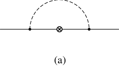
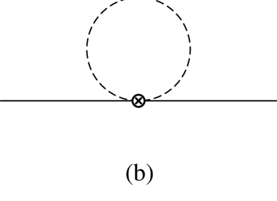
FIG. 1.: One-loop corrections to the baryon axial current.

FIG. 2.: Wave function renormalization of one-loop.

FIG. 3.: Best fit of baryon masses (tree) up to $O(\varepsilon^{5})$. Thick lines represent degenerate states.

FIG. 4.: One-loop corrections to the baryon mass. The filled-triangle denotes the mass insertion to the intermediate baryon state and the filled-box represents the meson-meson-baryon-baryon coupling from the chiral Lagrangian of (44) and (149).

	$\{{\cal U}\}$	$\{\sigma_{j}\}\{\sigma_{j}\}$	$\{{\cal S}\}$	$\{{\cal S}\}\{{\cal S}\}$	$\{{\cal S}\sigma_{j}\}\{\sigma_{j}\}$	$\{{\cal U}\sigma_{j}\}\{{\cal S}\sigma_{j}\}$
$N$	$2n+1$	3	0	0	0	0
$\Lambda$	$2n$	3	1	1	3	0
$\Sigma$	$2n$	3	1	1	$-1$	$-4$
$\Xi$	$2n-1$	3	2	4	4	$-4$
$\Delta$	$2n+1$	15	0	0	0	0
$\Sigma^{*}$	$2n$	15	1	1	5	2
$\Xi^{*}$	$2n-1$	15	2	4	10	2
$\Omega$	$2n-2$	15	3	9	15	0
$\tilde{\Xi}$	$2n-1$	$3$	$2$	$4$	$-2$	$-10$
$\tilde{\Omega}$	$2n-2$	$3$	$3$	$9$	$5$	$-10$
$\tilde{\Sigma}^{*}$	$2n$	$15$	$1$	$1$	$-3$	$-6$
$\tilde{\Xi}^{*}$	$2n-1$	$15$	$2$	$4$	$4$	$-4$
$\tilde{\Omega}^{*}$	$2n-2$	$15$	$3$	$9$	$11$	$-4$
$\tilde{\rm S}^{*}$	$2n-3$	$15$	$4$	$16$	$18$	$-6$
$\tilde{\Delta}^{**}$	$2n+1$	$35$	$0$	$0$	$0$	$0$
$\tilde{\Sigma}^{**}$	$2n$	$35$	$1$	$1$	$7$	$4$
$\tilde{\Xi}^{**}$	$2n-1$	$35$	$2$	$4$	$14$	$6$
$\tilde{\Omega}^{**}$	$2n-2$	$35$	$3$	$9$	$21$	$6$
$\tilde{\rm S}^{**}$	$2n-3$	$35$	$4$	$16$	$28$	$4$

TABLE I.: Matrix elements of various operators for baryon states

Particle	$O(\varepsilon^{1})$	$O(\varepsilon^{2})$	$O(\varepsilon^{3,4})$	$O(\varepsilon^{5})$	Expt.
$N$	1142	982	939	937	939
$\Lambda$	1142	1141	1117	1119	1116
$\Sigma$	1142	1141	1183	1183	1193
$\Xi$	1142	1300	1328	1327	1318
$\Delta$	1456	1217	1238	1236	1232
$\Sigma^{*}$	1456	1376	1383	1386	1385
$\Xi^{*}$	1456	1535	1528	1530	1530
$\Omega$	1456	1694	1673	1670	1672
$\sqrt{\chi^{2}}$	424	79	16	15
$a$	1063.0	923.9	863.7	862.4
$b$	26.2	19.5	25.0	24.9
$c$	—	159.0	227.8	96.5
$d$	—	—	$-16.6$	51.8
$e$	—	—	—	$-70.4$
$f$	—	—	—	$-67.8$

TABLE II.: Best fit of baryon masses (tree) in the unit of MeV at each order of $\varepsilon$ using the formula (87).

operator	$g^{2}$ term	$gh$ term	$h^{2}$ term
${\cal O}^{\pi}$	$N_{c}^{2}$	$N_{c}^{0}$	$N_{c}^{-2}$
${\cal O}^{K}$	$N_{c}^{1}$	$N_{c}^{0}$	$N_{c}^{-1}$
${\cal O}^{\eta}$	$N_{c}^{0}$	$N_{c}^{0}$	$N_{c}^{0}$

TABLE III.: The leading order of operator ${\cal O}^{\Pi}$ depending on the coupling constants.