CP VIOLATION IN DECAYS Z $\rightarrow$ 4 JETS

ABSTRACT

We analyse CP-violating effects in Z $\rightarrow$ 4 jet decays, assuming the presence of CP-violating effective $Zb\bar{b}G$ and $Zb\bar{b}GG$ couplings. We discuss the influence of these couplings on the decay width. Furthermore, we propose various strategies of a direct search for such CP-violating couplings by using different CP-odd observables. The present data of LEP 1 should give significant information on the couplings.

1 Introduction

In electron-positron collider experiments at LEP and SLC, a large number of Z bosons has been collected so that the detailed study of the decays of the Z boson has been made possible [1]. An interesting topic is the test of CP symmetry in such Z decays. There is already a number of theoretical ([2]-[19] and references therein) and experimental [20]-[27] studies of this subject. In the present paper we will study a flavour-diagonal Z decay where CP-violating effects within the Standard Model (SM) are estimated to be very small [4]. Thus, looking for CP violation in such Z decays means looking for new physics beyond the SM.

For a model-independent systematic analysis of CP violation in Z decays we use the effective Lagrangian approach as described in [4, 9]. Of particular interest are Z decays involving heavy leptons or quarks. Thus, the process Z $\rightarrow b\bar{b}G$ which is sensitive to effective CP-violating couplings in the $Zb\bar{b}G$ vertex has been analysed theoretically in [15, 17] and experimentally in [22]. No significant deviation from the SM has been found.

Here we present an analysis of the 4 jet decays of the Z boson involving $b$ quarks. If CP-violating couplings are introduced in the $Zb\bar{b}G$ vertex, they will, because of gauge invariance of QCD, appear in the $Zb\bar{b}GG$ vertex as well. But the $Zb\bar{b}GG$ vertex could in principle contain new coupling parameters. The 4 jet analysis looks into both, 4- and 5-point vertices.

In this paper we present the results of our calculations of the process Z $\rightarrow$ 4 jets including CP-violating couplings, with at least two of the jets originating from a $b$ or $\bar{b}$ quark. The following three subprocesses contribute to the 4 jet decay:

$$e^{+}\,(p_{+})\;e^{-}\,(p_{-})\rightarrow Z\,(p)\rightarrow b\,(k_{-})\;\bar{b}\,(k_{+})\;G\,(k_{1})\;G\,(k_{2})\,,$$ (1)

$$e^{+}\,(p_{+})\;e^{-}\,(p_{-})\rightarrow Z\,(p)\rightarrow b\,(k_{-})\;\bar{b}\,(k_{+})\;b\,(q_{-})\;\bar{b}\,(q_{+})\,,$$ (2)

$$e^{+}\,(p_{+})\;e^{-}\,(p_{-})\rightarrow Z\,(p)\rightarrow b\,(k_{-})\;\bar{b}\,(k_{+})\;q\,(q_{-})\;\bar{q}\,(q_{+})$$ (3)

$$\hphantom{e^{+}\,(p_{+})\;e^{-}\,(p_{-})\rightarrow Z\,(p)\rightarrow b\,(k_{-})\;\bar{b}\,(k_{+}}(q=u,d,s,c)\,.$$

We will always assume unpolarized $e^{+}$, $e^{-}$ beams and show the results for each process individually as well as the results for the sum of them. In the experiments, of course, only the sum of the three processes can be observed easily.

In chapter 2 we explain the theoretical framework of our computations. Next, in chapter 3, we analyse the anomalous couplings for partons in the final state. First, we discuss anomalous contributions to the decay width. Then, we define different CP-odd tensor and vector observables and calculate their sensitivities to anomalous couplings. In order to find out how “good” for the measurement of the new couplings our observables are, we compare them to the optimal observables. In chapter 4 we study decay width, tensor, vector and optimal observables in four different scenarios for an experimental analysis. Finally, we compare our results with results of the 3 jet decay. Our conclusions can be found in chapter 5.

2 Effective Lagrangian Approach

For a model independent study of CP violation in 4 jet decays of the Z boson we use the effective Lagrangian approach as explained in [4]. We add to the SM Lagrangian ${\cal L}_{SM}$ a CP-violating term ${\cal L}_{CP}$ containing all CP-odd local operators with a mass dimension $d\leq 6$ (after electroweak symmetry breaking) that can be constructed with SM fields. The effective CP-violating Lagrangian relevant to our analysis is:

$${\cal L}_{CP}(x)=$$ (4)

$$- \frac{i}{2}\tilde{d}_{b}\>\bar{b}(x)\>\sigma^{\mu\nu}\>\gamma_{5}\>b(x)\;[\partial_{\mu}\>Z_{\nu}(x)-\partial_{\nu}\>Z_{\mu}(x)]$$

$$- \frac{i}{2}d_{b}^{\prime}\>\bar{b}(x)\>T^{a}\>\sigma^{\mu\nu}\>\gamma_{5}\>b(x)\>G^{a}_{\mu\nu}(x)$$

$$+ [\;h_{Vb}\>\bar{b}(x)\>T^{a}\>\gamma^{\nu}\>b(x)+h_{Ab}\>\bar{b}(x)\>T^{a}\>\gamma^{\nu}\>\gamma_{5}\>b(x)\;]\;Z^{\mu}(x)\>G^{a}_{\mu\nu}(x)\;\;,$$

where $b(x)$ denotes the b quark field, $Z^{\mu}(x)$ and $G^{a}_{\mu\nu}(x)$ represent the field of the Z boson and the field strength tensor of the gluon, respectively, and $T^{a}=\lambda^{a}/2$ are the generators of $SU(3)_{C}$ [28]. In (4) $\tilde{d}_{b}$ is the weak dipole moment, $d_{b}^{\prime}$ the chromoelectric dipole moment, and $h_{Vb}$, $h_{Ab}$ are CP-violating vector and axial vector chirality conserving coupling constants. As effective coupling constants in ${\cal L}_{CP}$ the parameters $\tilde{d}_{b}$, $d_{b}^{\prime}$, $h_{Vb}$, $h_{Ab}$ are real. They are related to form factors of vertices but should not be confused with the latter (cf. e. g. [18]).

Information on the spin of the final state partons in (1 – 3) is hardly available experimentally. Thus, we consider as observables only the parton’s energies and momenta. Then, effects linear in the dipole form factors $\tilde{d}_{b}$ and $d_{b}^{\prime}$ are suppressed by powers of $m_{b}/m_{Z}$. So angular correlations of the jets in Z $\rightarrow$ 4 jets are only sensitive to the couplings $h_{Vb}$ and $h_{Ab}$.

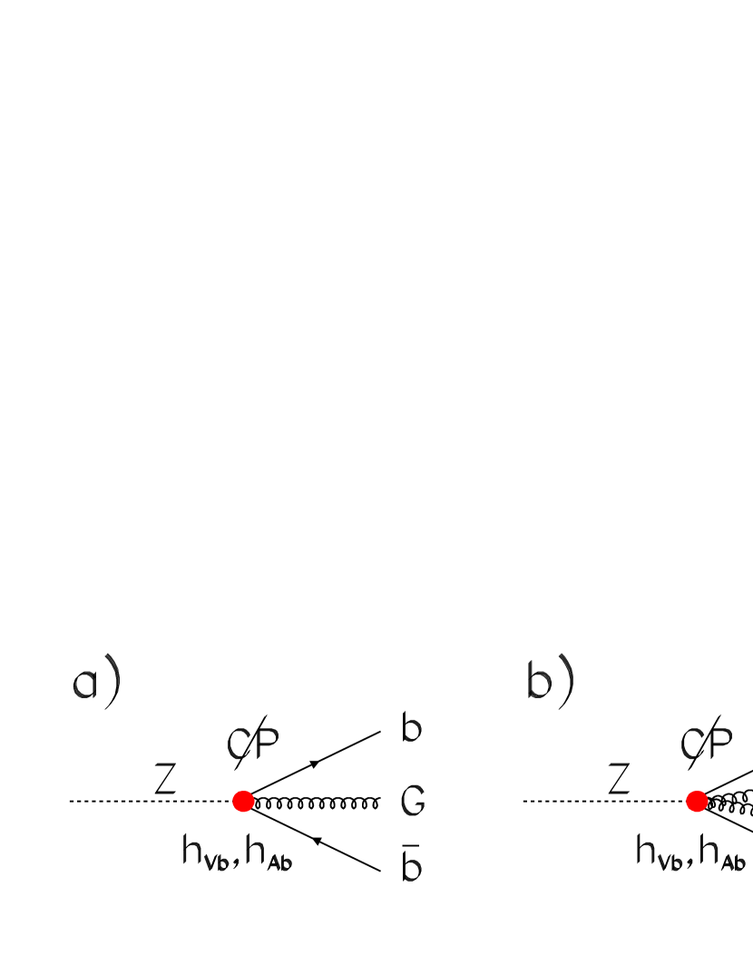
Figure 1: The CP-violating vertices.

The corresponding vertices following from ${\cal L}_{CP}$ are shown in figure 1. Because the non-abelian field strength tensor has a term quadratic in the gluon fields the $Zb\bar{b}G$- and $Zb\bar{b}GG$-vertices are related.

We define dimensionless coupling constants $\hat{h}_{Vb,Ab}$ using the Z mass as the scale parameter by

$$h_{Vb,Ab}=\frac{e\>g_{s}}{\sin\vartheta_{W}\>\cos\vartheta_{W}\>m_{Z}^{2}}\;\hat{h}_{Vb,Ab}\;.$$ (5)

For numerical calculations we set $m_{Z}=91.187\>$GeV, $\sin^{2}\vartheta_{W}=0.2236$ and the fine structure constant at the Z mass to $\alpha=1/128.9$ [29]. Our calculations are carried out in leading order of the CP-violating couplings of ${\cal L}_{CP}$ and the SM couplings. A non-vanishing $b$ quark mass of $4.5\>$GeV is included ; masses of $u$, $d$, $s$, $c$ quarks are neglected.

3 Study of CP-violating couplings for partons in the final state

In this chapter we discuss an ideal experiment where one is able to flavour-tag the partons and measure their momenta. We present a study of our CP-violating couplings for each process (1) – (3) separately and for the sum of them. We have computed the differential and integrated decay rates using FORM [31] and M [32] for the analytic and VEGAS [33] for the numerical calculation. We write the squared matrix element for each subprocess with final state $\mbox{$\wp$}={b\bar{b}GG},\;{b\bar{b}b\bar{b}},\;{b\bar{b}u\bar{u}},\;{b\bar{b}d\bar{d}},\;{b\bar{b}s\bar{s}},\;{b\bar{b}c\bar{c}}$ in the form:

$$R(\phi)^{(\mbox{$\wp$})} = S_{0}^{(\mbox{$\wp$})}(\phi)$$ (6)

$$+ \mbox{$\hat{h}_{b}$}S_{1}^{(\mbox{$\wp$})}(\phi)+\mbox{$\tilde{h}_{b}$}S_{2}^{(\mbox{$\wp$})}(\phi)$$

$$+ (\mbox{$\hat{h}_{Vb}$}^{2}+\mbox{$\hat{h}_{Ab}$}^{2})S_{3}^{(\mbox{$\wp$})}(\phi)+(\mbox{$\hat{h}_{Vb}$}^{2}-\mbox{$\hat{h}_{Ab}$}^{2})S_{4}^{(\mbox{$\wp$})}(\phi)+\mbox{$\hat{h}_{Vb}$}\mbox{$\hat{h}_{Ab}$}S_{5}^{(\mbox{$\wp$})}(\phi)\;.$$

Here $\phi$ stands collectively for the phase space variables, $S_{0}$ denotes the SM part and

$$\hat{h}_{b}=\hat{h}_{Ab}g_{Vb}-\hat{h}_{Vb}g_{Ab}\;,$$ (7)

$$\tilde{h}_{b}=\hat{h}_{Vb}g_{Vb}-\hat{h}_{Ab}g_{Ab}\;,$$ (8)

$$g_{Vb}=-\frac{1}{2}+\frac{2}{3}\sin^{2}\vartheta_{W}\;,\;\;g_{Ab}=-\frac{1}{2}\;.$$ (9)

In the following we drop the index $\wp$  if the given formula holds for the subprocesses and for the sum of the subprocesses.

The results within the SM have been compared analytically to calculations for vanishing b quark mass [34, 35] and to calculations for non-vanishing b quark mass [36]. Our results agree with these calculations.

The definition of a 4 jet sample requires the introduction of resolution cuts. We use JADE cuts [37] requiring

$$y_{ij}=\frac{2\,E_{i}E_{j}\,(1-\cos\vartheta_{ij})}{m_{Z}^{2}}>y_{cut}\;,$$ (10)

with $\vartheta_{ij}$ the angle between the momentum directions of any two partons ($i\neq j$) and $E_{i}$, $E_{j}$ their energies in the Z rest system. The expectation value of an observable ${\cal{O}}(\phi)$ is then defined as

$$<{\cal{O}}>=\frac{\int{\cal{O}}(\phi)\;R(\phi)\;d\phi}{\int R(\phi)\;d\phi}\,.$$ (11)

3.1 Anomalous contributions to the decay widths

The solid curves in figure 2 show the results of our calculations for the SM decay widths $\Gamma^{SM}$ as function of the jet resolution parameter $y_{cut}$ for the different processes. To check our calculations we computed $\Gamma^{SM}$ also with the program COMPHEP [38] and found — within numerical errors — complete agreement.

Figure 2: The decay width for different subprocesses as function of the jet resolution parameter $y_{cut}$ (10). The results for $Z\rightarrow b\bar{b}c\bar{c}$ ($b\bar{b}s\bar{s}$) are the same as for $Z\rightarrow b\bar{b}u\bar{u}$ ($b\bar{b}d\bar{d}$).

Figure 3: The different contributions to the 4 jet decay width as function of the jet resolution parameter for the sum of the processes (1 – 3).

As the decay width is a CP-even observable the contribution of the CP-violating interaction to it adds incoherently to the SM one [15]:

$$\Gamma=\Gamma^{SM}+\Delta\Gamma^{CP}\;,$$ (12)

with $\Delta\Gamma^{CP}$ being quadratic in the new couplings. In figure 2 the dashed curves represent $\Delta\Gamma^{CP}$ as function of $y_{cut}$ assuming $\hat{h}_{Vb}=\hat{h}_{Ab}=1/\sqrt{2}$.

As we can see, the dominant decay is (1). In comparison to this process, the processes (3) give only contributions at the per cent level, process (2) at the per mille level to the decay width. From (6) we find:

$$\Delta\Gamma^{CP}=(\mbox{$\hat{h}_{Vb}$}^{2}+\mbox{$\hat{h}_{Ab}$}^{2})\Gamma_{3}+(\mbox{$\hat{h}_{Vb}$}^{2}-\mbox{$\hat{h}_{Ab}$}^{2})\Gamma_{4}\;.$$ (13)

Because $S_{5}$ in (6) turns out to be odd under the exchange of quark and anti-quark momenta, its integral vanishes. In Figure 3, we compare for the sum of the processes (1 – 3) $\Gamma^{SM}$, $\Gamma_{3}$ and $\Gamma_{4}$. For $\hat{h}_{Vb}$, $\hat{h}_{Ab}$ of order one $\Delta\Gamma^{CP}$ is only a correction of a few per cent to $\Gamma^{SM}$ even if all processes (1 – 3) are added up. Thus, considering the theoretical uncertainties in the SM 4 jet decay rate, a determination of the new couplings by measuring the decay width alone does not look promising.

3.2 CP-odd observables

3.2.1 Tensor and vector observables

We now turn to a study of our CP-violating couplings using CP-odd observables constructed from the momentum directions of the $b$ and $\bar{b}$ quarks, $\hat{\bf k}_{b}={\bf k}_{b}/|{\bf k}_{b}|$ and $\hat{\bf k}_{\bar{b}}={\bf k}_{\bar{b}}/|{\bf k}_{\bar{b}}|$ (cf. [4, 9, 11, 17]):

$$T_{ij}^{(n)}=(\hat{\bf k}_{\bar{b}}-\hat{\bf k}_{b})_{i}\;(\hat{\bf k}_{\bar{b}}\times\hat{\bf k}_{b})_{j}\;|\hat{\bf k}_{\bar{b}}\times\hat{\bf k}_{b}|^{n-2}+(i\leftrightarrow j)\;,$$ (14)

$$V_{i}^{(n)}=(\hat{\bf k}_{\bar{b}}\times\hat{\bf k}_{b})_{i}\;|\hat{\bf k}_{\bar{b}}\times\hat{\bf k}_{b}|^{n-2}\;,$$ (15)

with $i$, $j$ the Cartesian vector indices in the Z rest system and $n=1,2,3$.

The observables $T_{ij}^{(n)}$ transform as tensors, $V_{i}^{(n)}$ as vectors. For unpolarized $e^{+}e^{-}$ beams and our rotationally invariant cuts (10) their expectation values are then proportional to the Z tensor polarization $S_{ij}$ and vector polarization $s_{i}$, respectively. Defining the positive $z$-axis in the $e^{+}$ beam direction, we have

$${\bf s}=\left(\begin{array}[]{c}0\\ 0\\ s_{3}\end{array}\right)\;,$$ (16)

$$(s_{ij})=\frac{1}{6}\left(\begin{array}[]{ccc}-1&0&0\\ 0&-1&0\\ 0&0&2\end{array}\right)\;,$$ (17)

where

$$s_{3}=\frac{2\,g_{Ve}g_{Ae}}{g_{Ve}^{2}+g_{Ae}^{2}}=0.209\;,$$ (18)

with $g_{Ve}=-1/2+2\sin^{2}\vartheta_{W}$ and $g_{Ae}=-1/2$ the weak vector and axial vector $Zee$ couplings. This shows that the components $T_{33}^{(n)}$ and $V_{3}^{(n)}$ are the most sensitive ones.

Note that the tensor observables do not change their sign upon charge misidentification ($\hat{\bf k}_{\bar{b}}\leftrightarrow\hat{\bf k}_{b}$) whereas the vector observables do. Thus, it is only for the measurement of the latter that charge identification is indispensable, which makes the vector observables less valuable for the experimental analysis.

We have computed the expectation values of the observables (14), (15) for different JADE cuts (10), as function of $\hat{h}_{b}$ (7) and $\tilde{h}_{b}$ (8). The expectation value of a CP-odd observable ${\cal{O}}$ has the following general form:

$$<\!{\cal{O}}\!>=(c_{1}\hat{h}_{b}+c_{2}\tilde{h}_{b})\,\frac{\Gamma^{SM}_{4\;jets}}{\Gamma_{4\;jets}}\;,$$ (19)

where $\Gamma^{SM}_{4\;jets}$ and $\Gamma_{4\;jets}$ denote the corresponding Z $\rightarrow$ 4 jets decay widths in the SM and in the theory with SM plus CP-violating couplings, respectively. In an experimental analysis $\Gamma^{SM}_{4\;jets}$ should be taken from the theoretical calculation, $\Gamma_{4\;jets}$ and $<\!{\cal{O}}\!>$ from the experimental measurement. The quantity $<\!{\cal{O}}\!>\!\cdot\,\Gamma_{4\;jets}$ is then an observable strictly linear in the anomalous couplings.

From the measurement of a single observable (19) we can get a simple estimate of its sensitivity to $\hat{h}_{b}$ by assuming $\mbox{$\tilde{h}_{b}$}=0$. The error on a measurement of $\hat{h}_{b}$ is then to leading order in the anomalous couplings:

$$\delta\hat{h}_{b}=\frac{\sqrt{<\!{\cal{O}}^{2}\!>_{SM}}}{|c_{1}|\sqrt{N}}\;,$$ (20)

where $N$ is the number of events within cuts. Similarly, assuming $\mbox{$\hat{h}_{b}$}=0$ we get the error on $\tilde{h}_{b}$ as

$$\delta\tilde{h}_{b}=\frac{\sqrt{<\!{\cal{O}}^{2}\!>_{SM}}}{|c_{2}|\sqrt{N}}\;.$$ (21)

A measure for the sensitivity of $\cal{O}$ to $\hat{h}_{b}$ ($\tilde{h}_{b}$) is then $1/\mbox{$\delta\hat{h}_{b}$}$ ($1/\mbox{$\delta\tilde{h}_{b}$}$). However, since we want to estimate 2 anomalous couplings $\hat{h}_{b}$, $\tilde{h}_{b}$ we should consider 2 linearly independent observables $\mbox{$\cal{O}$}_{1,2}$ such that:

$$<\!\mbox{$\cal{O}$}_{1}\!>=(\mbox{$\hat{h}_{b}$}c_{11}+\mbox{$\tilde{h}_{b}$}c_{12})\,\frac{\Gamma^{SM}_{4\;jets}}{\Gamma_{4\;jets}}\;,$$

$$<\!\mbox{$\cal{O}$}_{2}\!>=(\mbox{$\hat{h}_{b}$}c_{21}+\mbox{$\tilde{h}_{b}$}c_{22})\,\frac{\Gamma^{SM}_{4\;jets}}{\Gamma_{4\;jets}}\;.$$ (22)

The sensitivity of these observables to the anomalous couplings is estimated in the standard way. Neglecting terms quadratic in the anomalous couplings the combined measurement of $<\!\mbox{$\cal{O}$}_{1}\!>$ and $<\!\mbox{$\cal{O}$}_{2}\!>$ with a data sample of $N$ events (within the considered cuts) leads to an error ellipse

$$(\delta\mbox{$\hat{h}_{b}$})^{2}\,V(h)^{-1}_{11}+2\,\delta\mbox{$\hat{h}_{b}$}\delta\mbox{$\tilde{h}_{b}$}\,V(h)^{-1}_{12}+(\delta\mbox{$\tilde{h}_{b}$})^{2}\,V(h)^{-1}_{22}=1\;.$$ (23)

Here ${\sf V}(h)$ denotes the covariance matrix of the estimated couplings. We have in matrix notation:

$${\sf V}(h)=\frac{1}{N}{\sf c}^{-1}{\sf V}(\mbox{$\cal{O}$})({\sf c}^{-1})^{T}\;,$$ (24)

$${\sf c}=\left(\begin{array}[]{cc}c_{11}&c_{12}\\ c_{21}&c_{22}\end{array}\right)\;,$$ (25)

where

$$V(\mbox{$\cal{O}$})_{ij}=\frac{1}{\int S_{0}(\phi)d\phi}\int\mbox{$\cal{O}$}_{i}(\phi)\mbox{$\cal{O}$}_{j}(\phi)S_{0}(\phi)d\phi$$ (26)

are the elements of the covariance matrix of the observables $\mbox{$\cal{O}$}_{i}$, calculated in the SM. A measurement of $\hat{h}_{b}$, $\tilde{h}_{b}$ has to produce a mean value point outside the ellipse (23) to be able to claim a non-zero effect at the 1 s. d. level.

3.2.2 Optimal observables

In addition to the tensor and vector observables (14, 15) we study optimal observables, which have the largest possible statistical signal-to-noise ratio [39, 40, 41]. Neglecting higher orders in the anomalous couplings the optimal observables for measuring $\hat{h}_{b}$ and $\tilde{h}_{b}$ are obtained from the differential cross section (6) as

$$O_{i}(\phi)=\frac{S_{i}(\phi)}{S_{0}(\phi)}\;,\;\;\;\;(i=1,2)\;.$$ (27)

The expectation values for the optimal observables are as in (22) with the coefficient matrix elements

$$c_{ij}=\frac{1}{\int S_{0}d\phi}\int\frac{S_{i}(\phi)S_{j}(\phi)}{S_{0}(\phi)}d\phi\;.$$ (28)

For optimal observables we have

$$c_{ij}=V(\mbox{$\cal{O}$})_{ij}\;,$$ (29)

$$V(h)^{-1}_{ij}=Nc_{ij}\;.$$ (30)

3.2.3 Numerical results

We have calculated the sensitivities to $\hat{h}_{b}$ and $\tilde{h}_{b}$ for different tensor, vector and the optimal observables varying the jet resolution parameter $y_{cut}$ . We assume a total number of $10^{4}$ 4 jet events from (1 – 3) for $y_{cut}=0.01$:

$$N(y_{cut}=0.01)=10000\;.$$ (31)

The number of events for other values of $y_{cut}$ and for the various subprocesses is then calculated within the SM. The total number of Z decays corresponding to (31) is $N_{tot}\cong 6.4\cdot 10^{5}$.

For the process $Z\rightarrow b\bar{b}GG$, we found that, in very good approximation, the tensor observables are only sensitive to $\hat{h}_{b}$ and the vector observables only to $\tilde{h}_{b}$. The sensitivities to these CP-odd couplings as calculated from (20) and (21), respectively, are shown in figure 4. The sensitivity decreases with increasing $y_{cut}$ for all observables due to the decrease in number of events available. The differences due to the different weight factors for tensor and vector observables $T_{33}^{(n)}$, $V_{3}^{(n)}$ ($n=1,2,3$) are only small and all observables considered have nearly optimal sensitivities.

For the processes $Z\rightarrow b\bar{b}b\bar{b}$, $Z\rightarrow b\bar{b}u\bar{u}$ and $Z\rightarrow b\bar{b}d\bar{d}$ we present plots analogous to those for $Z\rightarrow b\bar{b}GG$ in figures 5 – 7. However, here the correlation of the sensitivity of $\hat{h}_{b}$ ($\tilde{h}_{b}$) with tensor (vector) observables no longer holds. In $Z\rightarrow b\bar{b}d\bar{d}$, for instance, the vector observables are more sensitive to $\hat{h}_{b}$ than to $\tilde{h}_{b}$. In the bottom of figure 7 we get a singularity for $\delta\tilde{h}_{b}$ because at $y_{cut}\approx 0.06$ the expectation values of our vector observables become zero. Left from the singularity all expectation values are negative, right from the singularity they are positive. For the sum of the processes the singularity in $\tilde{h}_{b}$ vanishes, because we have to add up both the variances of all subprocesses in the denominator and the expectation values of all subprocesses in the numerator of (21).

Two results are striking:

1. The sensitivities obtainable with optimal observables from the subprocesses (2, 3) are as good as or even better than those from (1) even if the number of events from (2, 3) represents only a small fraction of those from (1) (cf. figure 2).

2. For the processes (2, 3) the tensor and vector observables do not reach optimal sensitivities.

One may understand these points in the following way: In the Feynman graph giving the CP-violating amplitude for process (3), the gluon which comes out of the CP-violating vertex splits into a $q$ $\bar{q}$ pair. This means that the CP-violating vertex can be analysed not only by using the angular correlations of $b$ and $\bar{b}$ quark, but also, by means of the momentum directions of $q$ and $\bar{q}$ quarks. If the tensor and vector observables (14, 15) are used for the measurement all information on the CP-violating vertex delivered from the angular correlations of $q$ and $\bar{q}$ quarks is lost but, on the other hand, it is retained by the optimal observables. For process (2) this argumentation is similar.

In figure 8, results for the sum of the subprocesses (1 – 3) are shown for $y_{cut}=0.02$ for a combined measurement of $T_{33}^{(2)}$ (14) and $V_{3}^{(2)}$ (15) and for the optimal observables. The comparison of the solid bands (measurement of $T_{33}^{(2)}$ or $V_{3}^{(2)}$ alone, respectively) with the dashed lines corresponding to $\mbox{$\hat{h}_{b}$}=\pm 1$ and $\mbox{$\tilde{h}_{b}$}=\pm 1$ shows that $T_{33}^{(2)}$ is mostly sensitive to $\hat{h}_{b}$ and that $V_{3}^{(2)}$ is mostly sensitive to $\tilde{h}_{b}$. The comparison of the inner- and outermost ellipses shows that tensor and vector observables do not reach the optimal sensitivity for the sum of the processes (1 – 3). This is remarkable since for the dominant process (1) they do. Thus, as already discussed above, (2) and (3) which contribute little in the decay rate have a much larger influence in CP-odd observables. In tables 1, 2, 3 of appendix A, we list the elements of the coefficient matrix (25) and the covariance matrix (26) of the observables $\mbox{$\cal{O}$}_{1}=T_{33}^{(2)}$ (14), $\mbox{$\cal{O}$}_{2}=V_{3}^{(2)}$ (15) and the coefficient matrix elements (28) for the optimal observables (27) for different values of the jet resolution parameter $y_{cut}$ (10).

Figure 4: The inverse sensitivities of tensor, vector and optimal observables to $\hat{h}_{b}$ and $\tilde{h}_{b}$ (7,8) obtainable in $Z\rightarrow b\bar{b}GG$, as function of the jet resolution parameter $y_{cut}$ (10) assuming (31) for the number of events.

Figure 5: The inverse sensitivities of tensor, vector and optimal observables to $\hat{h}_{b}$ and $\tilde{h}_{b}$ (7,8) obtainable in $Z\rightarrow b\bar{b}b\bar{b}$, as function of the jet resolution parameter $y_{cut}$ (10) assuming (31) for the number of events.

Figure 6: The inverse sensitivities of tensor, vector and optimal observables to $\hat{h}_{b}$ and $\tilde{h}_{b}$ (7,8) obtainable in $Z\rightarrow b\bar{b}u\bar{u}$, as function of the jet resolution parameter $y_{cut}$ (10) assuming (31) for the number of events. The results for $Z\rightarrow b\bar{b}c\bar{c}$ are identical.

Figure 7: The inverse sensitivities of tensor, vector and optimal observables to $\hat{h}_{b}$ and $\tilde{h}_{b}$ (7,8) obtainable in $Z\rightarrow b\bar{b}d\bar{d}$, as function of the jet resolution parameter $y_{cut}$ (10) assuming (31) for the number of events. The results for $Z\rightarrow b\bar{b}s\bar{s}$ are identical.

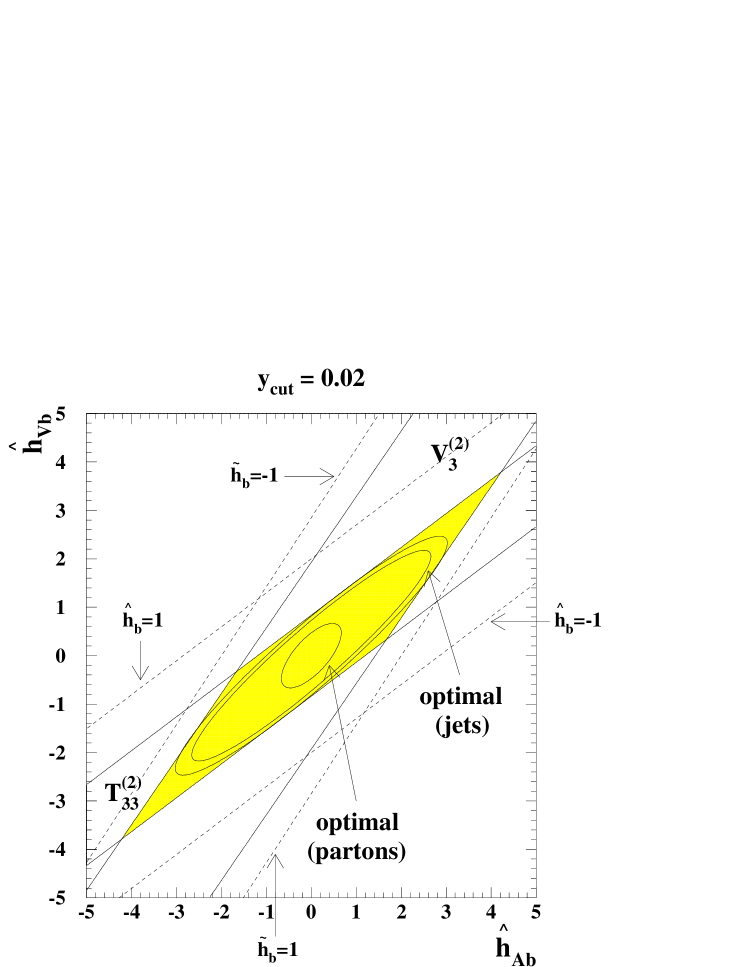
Figure 8: Contour plot for $y_{cut}=0.02$ of the 1 s. d. errors on $\hat{h}_{Vb}$, $\hat{h}_{Ab}$ as they can be obtained ideally from the measurement of different observables for Z $\rightarrow$ 4 jets. The innermost ellipsis is the result for the optimal observables $O_{1}$ and $O_{2}$ at parton level. The outermost ellipsis is the result for the combined measurement of $T_{33}^{(2)}$, $V_{3}^{(2)}$ at parton level. The solid bands correspond to a measurement of $T_{33}^{(2)}$ or $V_{3}^{(2)}$ alone, respectively. The overlap region of the tensor and vector errors is marked grey. The dashed lines correspond to $\mbox{$\hat{h}_{b}$}=\pm 1$ and $\mbox{$\tilde{h}_{b}$}=\pm 1$ as indicated. The ellipsis in the middle is the combined result for the optimal observables $O_{1}$ and $O_{2}$ for analysis 1 (cf. chapter 4).

4 CP-violating observables for jets

In an experimental analysis one can only measure jets as the “footprints” of the underlying partons, but not the partons themselves. So if we want to compare our calculations directly to experimental data, we must define observables for jets. In LEP experiments it is possible to tag a jet referring to a quark with b flavour [22]. In principle one can even distinguish between $b$ and $\bar{b}$ by measuring the jet charge, but this is difficult in practice. We propose four different types of analyses with the 4 jet data sample:

• Analysis 1: One jet comes from $b$ fragmentation, another from $\bar{b}$ fragmentation (double b tag); the other two jets (jets 3 and 4) are ordered according to the magnitude of their momenta.

For the next three analyses, we propose to make an ordering of all four jets according to the magnitude of their momenta:

$$|{\bf q}_{1}|\geq|{\bf q}_{2}|\geq|{\bf q}_{3}|\geq|{\bf q}_{4}|\;.$$ (32)

In the following we call jet 1 the jet with the highest magnitude of momentum, jet 2 the jet with the second highest magnitude of momentum and so on.

• Analysis 2: Jet 1 comes from $b$ or $\bar{b}$ fragmentation.

• Analysis 3: Jet 2 comes from $b$ or $\bar{b}$ fragmentation.

• Analysis 4: No requirement to the jet flavour (flavour blind case).

In appendix B we list the different classes of events for each of the subprocesses (1 – 3) as they contribute to these analyses.

In analyses 2 – 4 we do not distinguish between $b$ and $\bar{b}$ jets. It turns out that this in essence eliminates the dependence of the distributions on the CP-odd parameter $\tilde{h}_{b}$. Thus here we can only measure $\hat{h}_{b}$ and we set $\mbox{$\tilde{h}_{b}$}=0$ for these analyses.

4.1 Anomalous contributions to the decay width

We computed the total decay width for the 4 jet decays of the Z boson with at least two jets coming from $b$ or $\bar{b}$ fragmentation for the different analyses. Because a momentum ordering of jets can’t influence a decay rate, the analyses 1, 4 give results identical to those for the partons in the final state. In analyses 2, 3 some events are rejected as can be seen from the tables 9, 10, 11 of appendix B. The decay width must decrease in comparison to the other two analyses. Figure 9 shows this effect both for the SM contribution and for the contribution of the CP violating interaction to the decay width assuming $\mbox{$\hat{h}_{Vb}$}=\mbox{$\hat{h}_{Ab}$}=1/\sqrt{2}$.

Figure 9: The 4 jet decay width as function of the jet resolution parameter for different analyses. The three upper curves are the SM contributions, the others are the contributions from the CP-violating interaction if we set $\mbox{$\hat{h}_{Vb}$}=\mbox{$\hat{h}_{Ab}$}=1/\sqrt{2}$.

4.2 CP-odd observables

4.2.1 Tensor and vector observables

We found in chapter 3 that the observables $T_{33}^{(2)}$ (14) and $V_{3}^{(2)}$ (15) were the most sensitive ones. The same was found for the 3 jet decays (cf. [17]). Thus, from now on we concentrate on this type of observables.

Analysis 1:

The tensor and vector observables in this analysis are the same as for partons: $T_{33}^{(2)}$ (14) and $V_{3}^{(2)}$ (15). All results are identical to the parton case summed over the subprocesses (1 – 3) of chapter 3. Thus the sensitivity of a measurement of $T_{33}^{(2)}$ and $V_{3}^{(2)}$ to $\hat{h}_{Vb,Ab}$ for $y_{cut}=0.02$ is obtained from figure 8. For the measurement of the tensor observable, which is C-even, we do not need to distinguish between $\bar{b}$ and $b$ quark. A sufficient selection criterion is then that we demand two jets coming from $b$ or $\bar{b}$ fragmentation. For the measurement of the vector observable, which is C-odd, we need to distinguish between jets coming from $b$ or $\bar{b}$ fragmentation. This can be done experimentally by measuring the jet charge.

Analysis 2, 3, 4:

As tensor observable we chose now

$$T{{}^{\prime}}_{ij}^{(2)}=(\hat{\bf q}_{1}-\hat{\bf q}_{2})_{i}\;(\hat{\bf q}_{1}\times\hat{\bf q}_{2})_{j}+(i\leftrightarrow j)\;,$$ (33)

where $\hat{\bf q}_{i}={\bf q}_{i}/|{\bf q}_{i}|$. We computed the expectation values, variances etc. of the most sensitive component $i=j=3$ of these observables. All results are shown in figure 10. In table 4 in appendix A, we list the coefficients of the expectation values (19) for $\mbox{$\cal{O}$}=T{{}^{\prime}}_{33}^{(2)}$ (33) for different values of the jet resolution parameter $y_{cut}$ (10) for analysis 3.

Figure 10: The error (inverse sensitivity) $\delta\hat{h}_{b}$ obtainable from the tensor observable $T_{33}^{(2)}$ (14) from analysis 1 and $T{{}^{\prime}}_{33}^{(2)}$ (33) from analyses 2 – 4 as function of the jet resolution parameter $y_{cut}$ (10) assuming (31) for the number of events.

4.2.2 Optimal observables

The optimal observables are given in (27), where $\phi$ stands for the relevant phase space variables. Note that in calculating $S_{j}(\phi)$ ($j=0,1,2$) from (6) we have to sum over the subprocesses (1 – 3) taking into account how they contribute to the various analyses (tables 9 – 11).

In figure 8 we show the results for analysis 1 for $y_{cut}=0.02$ in the $\hat{h}_{Vb}$-$\hat{h}_{Ab}$-plane. Compared to the tensor and vector observables $T_{33}^{(2)}$, $V_{3}^{(2)}$ combined the optimal observables give only a marginal improvement now. This is in contrast to the partonic case and shows again that a lot of information about the CP-violating couplings is contained in the distribution of the secondary quark and anti quark in the subprocesses (2, 3). This information is washed out by assuming only knowledge of the momentum ordering of the two corresponding jets. We give the numerical values for the elements of the coefficient matrix (28) for the optimal observables (27) for different values of the jet resolution parameter $y_{cut}$ (10) for analysis 1 in table 5 of appendix A.

In figure 11 we show the inverse sensitivities $\delta\hat{h}_{b}$ for the optimal observable $O_{1}$ (cf. (27)) in the analyses 2 – 4, as function of the jet resolution parameter. It is interesting to note that using the tensor observable (33) analysis 3 is superior to 2 whereas with optimal observables the reverse is true. In table 6 of appendix A, we list the coefficients of the expectation values (19) for $\mbox{$\cal{O}$}=O_{1}$ (27) for different values of the jet resolution parameter $y_{cut}$ (10) for analysis 3.

Figure 11: The error $\delta\hat{h}_{b}$ obtainable from the optimal observable $O_{1}$ (27) from analyses 1 – 4 as function of the jet resolution parameter $y_{cut}$ (10) assuming (31) for the number of events.

4.3 Comparison with the decay Z $\rightarrow$ 3 jets

Since $\tilde{h}_{b}$ is in essence only measurable with $b$ and $\bar{b}$ distinction we concentrate on $\hat{h}_{b}$ in the following as measured with the tensor observables and the optimal observable $O_{1}$ in analyses 1 – 4. To compare the sensitivities of these analyses to those from the 3 jet analyses we calculate for each observable $\cal{O}$ the total number of Z events needed to measure $\hat{h}_{b}$ with a 1 s. d. accuracy $\delta\hat{h}_{b}$ within the cuts considered. In figures 12, 13 we show these results for analysis 1 and 3, respectively. Our results for the 3 jet analyses agree with the calculations [15, 17]. We see that the 4 jet analyses are competitive and even better than the 3 jet analyses for small values of the cut parameter $y_{cut}$. It should be noted, however, that our results concern the statistical errors only. Taking into account experimental efficiencies and systematic errors could change the situation considerably.

Figure 12: Comparison of the sensitivities of the best tensor observable $T_{33}^{(2)}$ (14) and the optimal observable $O_{1}$ (27) for the Z $\rightarrow$ 4 jets (analysis 1) with the best tensor observable $T_{33}^{(2)}$ (14) for the Z $\rightarrow$ 3 jets analysis (cf.[17]). The results for $|\mbox{$\hat{h}_{b}$}|^{2}N_{tot}$ are shown as function of the jet resolution parameter. $N_{tot}$ is the total number of Z decays required to see an effect at the 1 s. d. level for given $|\mbox{$\hat{h}_{b}$}|$.

Figure 13: Comparison of the sensitivities of the best tensor observable $T{{}^{\prime}}_{33}^{(2)}$ (33) and the optimal observable $O_{1}$ (27) for the Z $\rightarrow$ 4 jets (analysis 3) with the tensor observable $T{{}^{\prime}}_{33}^{(2)}$ (33) for the Z $\rightarrow$ 3 jets analysis (s. also [15, 17]). The results $|\mbox{$\hat{h}_{b}$}|^{2}N_{tot}$ are shown as function of the jet resolution parameter. $N_{tot}$ is the total number of Z decays required to see an effect at the 1 s. d. level for given $|\mbox{$\hat{h}_{b}$}|$.

5 Conclusions

In this paper, we have presented various calculations concerning the search for CP violation in the 4 jet decays of the Z boson with at least two of the jets originating from $b$ and $\bar{b}$ quarks. We have studied a CP-violating contact interaction with a vector and axial vector coupling $\hat{h}_{Vb}$, $\hat{h}_{Ab}$ (4). Such couplings can arise at one loop level in multi-Higgs extensions of the Standard Model [16, 42].

We found that, for reasonable values of the coupling constants, the additional contribution of the contact interaction to the decay width is at most at the percent level. The decay width alone is therefore not appropriate for determining the coupling constants.

We investigated tensor and vector as well as optimal observables which can be used for the measurement of the anomalous couplings. We studied different scenarios for an experimental analysis of the anomalous couplings: The ideal case where all the momenta and flavours of the partons can be reconstructed from the jets and four realistic cases where flavour information is available only for the $b$ jets.

If flavour tagging of all jets is available then, with a total number of Z decays $N_{tot}\cong 6.4\cdot 10^{5}$ and choosing a cut parameter $y_{cut}=0.02$ the anomalous coupling constants $\hat{h}_{b}$, $\tilde{h}_{b}$ (7, 8) can be determined with an accuracy of order 0.1 – 0.2 at 1 s. d. level using optimal observables (see figs. 4 - 8).

In the more realistic case where flavour tagging is available only for $b$ and $\bar{b}$ jets, the coupling constant $\hat{h}_{b}$ can be measured with an accuracy of order 0.5 – 0.6 using the same total number of Z decays. In such a measurement $b-\mbox{$\bar{b}$}$ distinction is not necessary. Using in particular the simple tensor observable $T_{33}^{(2)}$ (14) for the measurement, an almost optimal sensitivity to $\hat{h}_{b}$ can be attained.

If $b-\mbox{$\bar{b}$}$ distinction is experimentally realizable, the coupling constant $\tilde{h}_{b}$ can be measured with an accuracy of order 0.8 . Again we found a simple vector observable $V_{3}^{(2)}$ (15) with an almost optimal sensitivity to $\tilde{h}_{b}$. If $b-\mbox{$\bar{b}$}$ distinction is experimentally not realizable the coupling constant $\tilde{h}_{b}$ remains essentially unconstrained from measurements of CP-odd observables. It can be bounded indirectly by assuming, for instance, that its contribution to the 4 jet width does not exceed $5\%$. This implies then $|\mbox{$\tilde{h}_{b}$}|\raisebox{-1.72218pt}{\hbox to0.0pt{$\sim$\hss}}\raisebox{1.72218pt}{$<$}\,O(1)$.

In our theoretical investigations we assumed always $100\%$ efficiencies and considered the statistical errors only. But the total number of Z decays collected by the LEP and SLC experiments together is of order $10^{7}$. Thus the accuracies in the determinations of $\hat{h}_{b}$, $\tilde{h}_{b}$ discussed above should indeed be within experimental reach.

Comparing 3 and 4 jet analyses we found that the sensitivity to the anomalous coupling $\hat{h}_{b}$ was roughly constant as function of the cut parameter $y_{cut}$ for $\mbox{$y_{cut}$}<0.1$ in the 3 jet case. For the 4 jet case the sensitivity was found to increase as $y_{cut}$ decreases. For $\mbox{$y_{cut}$}\,\raisebox{-1.72218pt}{\hbox to0.0pt{$\sim$\hss}}\raisebox{1.72218pt}{$<$}\,0.01$ the 4 jet sensitivity was found to exceed that from 3 jets (figures 12, 13). Of course in an experimental analysis one should try to make both 3 and 4 jet analyses in order to extract the maximal possible information from the data.

For the experimental analyses, one usually has to make Monte Carlo simulations. For this purpose one needs matrix elements including the CP-violating interaction. These are available from us in the form of FORTRAN subroutines.

To conclude: we have discussed in detail various possibilities to determine or obtain limits on anomalous CP-violating $Zb\bar{b}G$ and $Zb\bar{b}GG$ couplings. As shown in [16, 42] this will give valuable information on the scalar sector in multi-Higgs extensions of the Standard Model.

Acknowledgements

We would like to thank W. Bernreuther, A. Brandenburg, S. Dhamotharan, M. Diehl, P. Haberl, W. Kilian, J. von Krogh, R. Liebisch, P. Overmann, S. Schmitt, M. Steiert, D. Topaj and M. Wunsch for valuable discussions.

Appendix A Numerical Values

We list some numerical results for the coefficient matrices and covariance matrices in different studies. The statistical errors of the numerical calculation are typically at the per cent level.

$y_{cut}$	$c_{11}$	$c_{12}$	$c_{21}$	$c_{22}$
0.01	$-0.01827$	$-2.496\cdot 10^{-5}$	$-3.556\cdot 10^{-4}$	$6.426\cdot 10^{-3}$
0.02	$-0.02320$	$-6.706\cdot 10^{-5}$	$-4.504\cdot 10^{-4}$	$8.336\cdot 10^{-3}$
0.05	$-0.03253$	$-1.666\cdot 10^{-4}$	$-7.127\cdot 10^{-4}$	$0.01248$

Table 1: The numerical values for the elements of the coefficient matrix (25) of the observables $\mbox{$\cal{O}$}_{1}=T_{33}^{(2)}$ (14), $\mbox{$\cal{O}$}_{2}=V_{3}^{(2)}$ (15) for different values of the jet resolution parameter $y_{cut}$ (10) for partons in the final state (section 3).

$y_{cut}$	$V(\mbox{$\cal{O}$})_{11}$	$V(\mbox{$\cal{O}$})_{12}=V(\mbox{$\cal{O}$})_{21}$	$V(\mbox{$\cal{O}$})_{22}$
0.01	0.2772	0.01811	0.1109
0.02	0.3429	0.02334	0.1427
0.05	0.4332	0.02949	0.1959

Table 2: The numerical values for the elements of the covariance matrix (26) of the observables $\mbox{$\cal{O}$}_{1}=T_{33}^{(2)}$ (14), $\mbox{$\cal{O}$}_{2}=V_{3}^{(2)}$ (15) for different values of the jet resolution parameter $y_{cut}$ (10) for partons in the final state (section 3).

$y_{cut}$	$c_{11}$	$c_{12}=c_{21}$	$c_{22}$
0.01	$5.556\cdot 10^{-3}$	$3.228\cdot 10^{-3}$	$4.726\cdot 10^{-3}$
0.02	$9.557\cdot 10^{-3}$	$6.698\cdot 10^{-3}$	$9.588\cdot 10^{-3}$
0.05	0.02274	0.02002	0.02816

Table 3: The numerical values for the elements of the coefficient matrix (28) for the optimal observables (27) for different values of the jet resolution parameter $y_{cut}$ (10) for partons in the final state (section 3).

$y_{cut}$	$c_{1}$
0.01	$-0.01020$
0.02	$-0.01256$
0.05	$-0.01502$

Table 4: The numerical values the coefficients of the expectation values (19) for $\mbox{$\cal{O}$}=T{{}^{\prime}}_{33}^{(2)}$ (33) for different values of the jet resolution parameter $y_{cut}$ (10) for analysis 3 of section 4.

$y_{cut}$	$c_{11}$	$c_{12}=c_{21}$	$c_{22}$
0.01	$1.514\cdot 10^{-3}$	$1.041\cdot 10^{-4}$	$4.825\cdot 10^{-4}$
0.02	$1.981\cdot 10^{-3}$	$1.651\cdot 10^{-4}$	$6.396\cdot 10^{-4}$
0.05	$2.956\cdot 10^{-3}$	$3.042\cdot 10^{-4}$	$9.907\cdot 10^{-4}$

Table 5: The numerical values for the elements of the coefficient matrix (28) for the optimal observables (27) for different values of the jet resolution parameter $y_{cut}$ (10) for analysis 1 of section 4.

$y_{cut}$	$c_{1}$
0.01	$5.535\cdot 10^{-4}$
0.02	$7.124\cdot 10^{-4}$
0.05	$8.627\cdot 10^{-4}$

Table 6: The numerical values for the coefficients of the expectation values (19) for the optimal observable $\mbox{$\cal{O}$}=O_{1}$ (27) for different values of the jet resolution parameter $y_{cut}$ (10) for analysis 3 of section 4.

Appendix B Eventclasses

Here we explain which classes of events contribute to the four different analyses as defined in chapter 4. First, we compare the partonic phase space with the jet phase space.

Process	Phase space restriction
$e^{+}e^{-}\rightarrow Z\rightarrow b\bar{b}GG$	$|{\bf k}_{1}|\geq|{\bf k}_{2}|$
$e^{+}e^{-}\rightarrow Z\rightarrow b\bar{b}b\bar{b}$	$|{\bf k}_{+}|\geq|{\bf q}_{+}|$, $|{\bf k}_{-}|\geq|{\bf q}_{-}|$
$e^{+}e^{-}\rightarrow Z\rightarrow b\bar{b}q\bar{q}$	—

Table 7: The restrictions on the partonic phase space for the different processes due to identical particles in the final state.

Analysis	Phase space restriction
1	$|{\bf q}_{3}|\geq|{\bf q}_{4}|$
2, 3, 4	$|{\bf q}_{1}|\geq|{\bf q}_{2}|\geq|{\bf q}_{3}|\geq|{\bf q}_{4}|$

Table 8: The restrictions on the jet phase space in the analyses 1 – 4.

In Tables 7, 8 we list the restrictions on the phase space for the partonic processes (1 – 3) and for the jets in the analyses 1 – 4 as defined in chapter 4.

In tables 9 – 11 we list all possibilities how the 4 partons of the reactions (1 – 3) can give 4 jets with the ordering criteria of the analyses 1 – 4. The full points indicate that an event class satisfies the respective selection criterion.

$\bar{b}$ jet	$b$ jet	jet 3	jet 4	Analysis 1
$\mbox{$\bar{b}$}(k_{+})$	$b(k_{-})$	$G(k_{1})$	$G(k_{2})$	$\bullet$

jet 1	jet 2	jet 3	jet 4	Analysis 2	Analysis 3	Analysis 4
$\bar{b}(k_{+})$	$b(k_{-})$	$G(k_{1})$	$G(k_{2})$	$\bullet$	$\bullet$	$\bullet$
$\bar{b}(k_{+})$	$G(k_{1})$	$b(k_{-})$	$G(k_{2})$	$\bullet$		$\bullet$
$\bar{b}(k_{+})$	$G(k_{1})$	$G(k_{2})$	$b(k_{-})$	$\bullet$		$\bullet$
$b(k_{-})$	$\bar{b}(k_{+})$	$G(k_{1})$	$G(k_{2})$	$\bullet$	$\bullet$	$\bullet$
$b(k_{-})$	$G(k_{1})$	$\bar{b}(k_{+})$	$G(k_{2})$	$\bullet$		$\bullet$
$b(k_{-})$	$G(k_{1})$	$G(k_{2})$	$\bar{b}(k_{+})$	$\bullet$		$\bullet$
$G(k_{1})$	$\bar{b}(k_{+})$	$b(k_{-})$	$G(k_{2})$		$\bullet$	$\bullet$
$G(k_{1})$	$\bar{b}(k_{+})$	$G(k_{2})$	$b(k_{-})$		$\bullet$	$\bullet$
$G(k_{1})$	$b(k_{-})$	$\bar{b}(k_{+})$	$G(k_{2})$		$\bullet$	$\bullet$
$G(k_{1})$	$b(k_{-})$	$G(k_{2})$	$\bar{b}(k_{+})$		$\bullet$	$\bullet$
$G(k_{1})$	$G(k_{2})$	$\bar{b}(k_{+})$	$b(k_{-})$			$\bullet$
$G(k_{1})$	$G(k_{2})$	$b(k_{-})$	$\bar{b}(k_{+})$			$\bullet$

Table 9: The only possibility for the partons in $e^{+}e^{-}\rightarrow Z\rightarrow b\bar{b}GG$ to fulfill the selection criterion of analysis 1 and the 12 possibilities for them to give 4 momentum ordered jets. It is indicated by dots which event class contributes to which of the analyses.

$\bar{b}$ jet	$b$ jet	jet 3	jet 4	Analysis 1
$\mbox{$\bar{b}$}(k_{+})$	$b(k_{-})$	$b(q_{-})$	$\mbox{$\bar{b}$}(q_{+})$	$\bullet$
$\mbox{$\bar{b}$}(k_{+})$	$b(k_{-})$	$\mbox{$\bar{b}$}(q_{+})$	$b(q_{-})$	$\bullet$
$\mbox{$\bar{b}$}(q_{+})$	$b(k_{-})$	$b(q_{-})$	$\mbox{$\bar{b}$}(k_{+})$	$\bullet$
$\mbox{$\bar{b}$}(q_{+})$	$b(k_{-})$	$\mbox{$\bar{b}$}(k_{+})$	$b(q_{-})$	$\bullet$
$\mbox{$\bar{b}$}(k_{+})$	$b(q_{-})$	$b(k_{-})$	$\mbox{$\bar{b}$}(q_{+})$	$\bullet$
$\mbox{$\bar{b}$}(k_{+})$	$b(q_{-})$	$\mbox{$\bar{b}$}(q_{+})$	$b(k_{-})$	$\bullet$
$\mbox{$\bar{b}$}(q_{+})$	$b(q_{-})$	$b(k_{-})$	$\mbox{$\bar{b}$}(k_{+})$	$\bullet$
$\mbox{$\bar{b}$}(q_{+})$	$b(q_{-})$	$\mbox{$\bar{b}$}(k_{+})$	$b(k_{-})$	$\bullet$

jet 1	jet 2	jet 3	jet 4	Analysis 2	Analysis 3	Analysis 4
$\bar{b}(k_{+})$	$b(k_{-})$	$b(q_{-})$	$\bar{b}(q_{+})$	$\bullet$	$\bullet$	$\bullet$
$\bar{b}(k_{+})$	$b(k_{-})$	$\bar{b}(q_{+})$	$b(q_{-})$	$\bullet$	$\bullet$	$\bullet$
$\bar{b}(k_{+})$	$\bar{b}(q_{+})$	$b(k_{-})$	$b(q_{-})$	$\bullet$	$\bullet$	$\bullet$
$b(k_{-})$	$\bar{b}(k_{+})$	$b(q_{-})$	$\bar{b}(q_{+})$	$\bullet$	$\bullet$	$\bullet$
$b(k_{-})$	$\bar{b}(k_{+})$	$\bar{b}(q_{+})$	$b(q_{-})$	$\bullet$	$\bullet$	$\bullet$
$b(k_{-})$	$b(q_{-})$	$\bar{b}(k_{+})$	$\bar{b}(q_{+})$	$\bullet$	$\bullet$	$\bullet$

Table 10: The 8 possibilities for the partons in $e^{+}e^{-}\rightarrow Z\rightarrow b\bar{b}b\bar{b}$ to fulfill the selection criterion of analysis 1 and the 6 possibilities for them to give 4 momentum ordered jets. It is indicated by dots which event class contributes to which of the analyses.

$\bar{b}$ jet	$b$ jet	jet 3	jet 4	Analysis 1
$\mbox{$\bar{b}$}(k_{+})$	$b(k_{-})$	$q(q_{-})$	$\mbox{$\bar{q}$}(q_{+})$	$\bullet$
$\mbox{$\bar{b}$}(k_{+})$	$b(k_{-})$	$\mbox{$\bar{q}$}(q_{+})$	$q(q_{-})$	$\bullet$

jet 1	jet 2	jet 3	jet 4	Analysis 2	Analysis 3	Analysis 4
$\bar{b}(k_{+})$	$b(k_{-})$	$q(q_{-})$	$\mbox{$\bar{q}$}(q_{+})$	$\bullet$	$\bullet$	$\bullet$
$\bar{b}(k_{+})$	$b(k_{-})$	$\mbox{$\bar{q}$}(q_{+})$	$q(q_{-})$	$\bullet$	$\bullet$	$\bullet$
$\bar{b}(k_{+})$	$q(q_{-})$	$b(k_{-})$	$\mbox{$\bar{q}$}(q_{+})$	$\bullet$		$\bullet$
$\bar{b}(k_{+})$	$\mbox{$\bar{q}$}(q_{+})$	$b(k_{-})$	$q(q_{-})$	$\bullet$		$\bullet$
$\bar{b}(k_{+})$	$q(q_{-})$	$\mbox{$\bar{q}$}(q_{+})$	$b(k_{-})$	$\bullet$		$\bullet$
$\bar{b}(k_{+})$	$\mbox{$\bar{q}$}(q_{+})$	$q(q_{-})$	$b(k_{-})$	$\bullet$		$\bullet$
$b(k_{-})$	$\bar{b}(k_{+})$	$q(q_{-})$	$\mbox{$\bar{q}$}(q_{+})$	$\bullet$	$\bullet$	$\bullet$
$b(k_{-})$	$\bar{b}(k_{+})$	$\mbox{$\bar{q}$}(q_{+})$	$q(q_{-})$	$\bullet$	$\bullet$	$\bullet$
$b(k_{-})$	$q(q_{-})$	$\bar{b}(k_{+})$	$\mbox{$\bar{q}$}(q_{+})$	$\bullet$		$\bullet$
$b(k_{-})$	$\mbox{$\bar{q}$}(q_{+})$	$\bar{b}(k_{+})$	$q(q_{-})$	$\bullet$		$\bullet$
$b(k_{-})$	$q(q_{-})$	$\mbox{$\bar{q}$}(q_{+})$	$\bar{b}(k_{+})$	$\bullet$		$\bullet$
$b(k_{-})$	$\mbox{$\bar{q}$}(q_{+})$	$q(q_{-})$	$\bar{b}(k_{+})$	$\bullet$		$\bullet$
$q(q_{-})$	$\bar{b}(k_{+})$	$b(k_{-})$	$\mbox{$\bar{q}$}(q_{+})$		$\bullet$	$\bullet$
$\mbox{$\bar{q}$}(q_{+})$	$\bar{b}(k_{+})$	$b(k_{-})$	$q(q_{-})$		$\bullet$	$\bullet$
$q(q_{-})$	$\bar{b}(k_{+})$	$\mbox{$\bar{q}$}(q_{+})$	$b(k_{-})$		$\bullet$	$\bullet$
$\mbox{$\bar{q}$}(q_{+})$	$\bar{b}(k_{+})$	$q(q_{-})$	$b(k_{-})$		$\bullet$	$\bullet$
$q(q_{-})$	$b(k_{-})$	$\bar{b}(k_{+})$	$\mbox{$\bar{q}$}(q_{+})$		$\bullet$	$\bullet$
$\mbox{$\bar{q}$}(q_{+})$	$b(k_{-})$	$\bar{b}(k_{+})$	$q(q_{-})$		$\bullet$	$\bullet$
$q(q_{-})$	$b(k_{-})$	$\mbox{$\bar{q}$}(q_{+})$	$\bar{b}(k_{+})$		$\bullet$	$\bullet$
$\mbox{$\bar{q}$}(q_{+})$	$b(k_{-})$	$q(q_{-})$	$\bar{b}(k_{+})$		$\bullet$	$\bullet$
$q(q_{-})$	$\mbox{$\bar{q}$}(q_{+})$	$\bar{b}(k_{+})$	$b(k_{-})$			$\bullet$
$\mbox{$\bar{q}$}(q_{+})$	$q(q_{-})$	$\bar{b}(k_{+})$	$b(k_{-})$			$\bullet$
$q(q_{-})$	$\mbox{$\bar{q}$}(q_{+})$	$b(k_{-})$	$\bar{b}(k_{+})$			$\bullet$
$\mbox{$\bar{q}$}(q_{+})$	$q(q_{-})$	$b(k_{-})$	$\bar{b}(k_{+})$			$\bullet$

Table 11: The 2 possibilities for the partons in $e^{+}e^{-}\rightarrow Z\rightarrow b\bar{b}q\bar{q}$ to fulfill the selection criterion of analysis 1 and the 24 possibilities for them to give 4 momentum ordered jets. It is indicated by dots which event class contributes to which of the analyses.

References

• [1] The LEP Collaborations ALEPH, DELPHI, L3, OPAL and the LEP Electroweak Working Group, and the SLD Heavy Flavour Group, A Combination of Preliminary LEP Electroweak Measurements and Constraints on the Standard Model, CERN-PPE/97-154.
• [2] L. Stodolsky: Phys. Lett. B 150 (1985) 221;
F. Hoogeveen, L. Stodolsky: Phys. Lett. B 212 (1988) 505.
• [3] J. F. Donoghue, B. R. Holstein, G. Valencia: Int. J. Mod. Phys. A 2 (1987) 319;
J. F. Donoghue, G. Valencia: Phys. Rev. Lett. 58 (1987) 451.
• [4] W. Bernreuther, U. Löw, J. P. Ma, O. Nachtmann: Z. Phys. C 43 (1989) 117.
• [5] J. Bernabéu, N. Rius: Phys. Lett. 232 (1989) 127;
J. Bernabéu, N. Rius, A. Pich: Phys. Lett. 257 (1991) 219.
• [6] M. B. Gavela, F. Iddir, A. Le Yaouanc, L. Olivier, O. Pène, J. C. Raynal: Phys. Rev. D 39 (1989) 1870;
A. De Rujula, M. B. Gavela, O. Pène, F. J. Vegas: Nucl. Phys. B 357 (1991) 311.
• [7] S. Goozovat, C. A. Nelson: Phys. Lett. B 267 (1991) 128;
Phys. Rev. D 44 (1991) 311.
• [8] W. Bernreuther, O. Nachtmann: Phys. Rev. Lett. 63 (1989) 2787.
• [9] J. Körner, J. P. Ma, R. Münch, O. Nachtmann, R. Schöpf: Z. Phys. C 49 (1991) 447.
• [10] W. Bernreuther, G.W. Botz, O. Nachtmann, P. Overmann: Z. Phys. C 52 (1991) 567.
• [11] W. Bernreuther, O. Nachtmann: Phys. Lett. B 268 (1991) 424.
• [12] G. Valencia, A. Soni: Phys. Lett. B 263 (1991) 517.
• [13] W. Bernreuther, O. Nachtmann, P. Overmann: Phys. Rev. D 48 (1993) 78.
• [14] K. J. Abraham, B. Lampe: Phys. Lett. B 326 (1994) 175.
• [15] W. Bernreuther, G. W. Botz, D. Bruß, P. Haberl, O. Nachtmann: Z. Phys. C 68 (1995) 73.
• [16] W. Bernreuther, A. Brandenburg, P. Haberl, O. Nachtmann: Phys. Lett. B 387 (1996) 155.
• [17] P. Haberl: “CP Violating Couplings in Z $\rightarrow$ 3 Jet Decays Revisited”, hep-ph/9611430.
• [18] W. Bernreuther, O. Nachtmann: Z. Phys. C 73 (1997) 647.
• [19] D. Bruß, O. Nachtmann, P. Overmann: Eur. Phys. J. C 1 (1998) 191.
• [20] D. Buskulic et al., (ALEPH Collaboration): Phys. Lett. B 297 (1992) 459.
• [21] D. Buskulic et al., (ALEPH Collaboration): Phys. Lett. B 346 (1995) 371.
• [22] D. Buskulic et al., (ALEPH Collaboration): Phys. Lett. B 384 (1996) 365.
• [23] M. Acciarri et al., (L3 Collaboration): Phys. Lett B 436 (1998) 428.
• [24] P.D. Acton et al., (OPAL Collaboration): Phys. Lett. B 281 (1992) 405.
• [25] R. Akers et al., (OPAL Collaboration): Z. Phys. C 66 (1995) 31.
• [26] K. Ackerstaff et al., (OPAL Collaboration): Z. Phys. C 74 (1997) 403.
• [27] M. Steiert: “Suche nach CP-verletzenden Effekten in hadronischen 3-Jet Ereignissen mit bottom Flavour $Z^{0}\rightarrow b\bar{b}G$”, Diploma thesis, University of Heidelberg (unpublished);
Rainer Liebisch: “Suche nach CP-verletzenden Effekten außerhalb des Standardmodells im Zerfall $Z^{0}\rightarrow b\bar{b}g$”, Diploma thesis, University of Heidelberg (unpublished).
• [28] Otto Nachtmann: “Elementary Particle Physics”, Springer, Berlin 1990.
• [29] R. M. Barnett et al. (PDG): Phys. Rev. D 54 (1996) 1.
• [30] M. Bilenky, G. Rodrigo, A. Santamaria: “NLO Calculations of the Three Jet Heavy Quark Production in $e^{+}e^{-}$ Annihilation: Status and Applications”, hep-ph/9811465.
M. Jamin: “Quark masses”, talk given at the conference “Quarks in Hadrons and Nuclei”, Oberwölz, September 1998 (to be published in the Proceedings).
• [31] The Symbolic Manipulation Program FORM. By J.A.M. Vermaseren (KEK, Tsukuba). KEK-TH-326, Mar 1992. 20pp.
• [32] P. Overmann, private communication, M - Reference Manual,
http://www.thphys.uni-heidelberg.de/$\>\tilde{}\,$overmann/M.html.
• [33] VEGAS: An Adaptive Multidimensional Integration Program. By G.Peter Lepage (Cornell U., LNS). CLNS-80/447, Mar 1980. 30pp.
• [34] A. Reiter: “QCD-Untersuchungen zur Elektron-Positron-Annihilation in 4 Jets”, Diploma thesis, University of Heidelberg (unpublished);
A. Reiter: Doctoral thesis, University of Heidelberg (1982).
• [35] O. Nachtmann, A. Reiter: Z.Phys. C 14 (1982) 47;
O. Nachtmann, A. Reiter: Z.Phys. C 16 (1982) 45.
• [36] A. Brandenburg, P. Uwer: Nucl. Phys. B 515 (1998) 279.
• [37] S. Bethke et al. (JADE Collaboration): Phys. Lett. B 213 (1988) 235.
• [38] P.A.Baikov et al., Physical Results by means of CompHEP, in Proc.of X Workshop on High Energy Physics and Quantum Field Theory (QFTHEP-95), ed.by B.Levtchenko, V.Savrin, Moscow: hep-ph/9701412 (1996) 101;
E.E.Boos, M.N.Dubinin, V.A.Ilyin, A.E.Pukhov, V.I.Savrin: hep-ph/9503280.
• [39] D. Atwood, A. Soni: Phys. Rev. D 45 (1992) 2405;
M. Davier, L. Duflot, F. Le Diberder, A. Rougé: Phys. Lett. B 306 (1993) 411.
• [40] M. Diehl, O. Nachtmann: Z. Phys. C 62 (1994) 397.
• [41] M. Diehl, O. Nachtmann: Eur. Phys. J. C 1 (1998) 177.
• [42] W. Bernreuther, O. Nachtmann: “Flavor Dynamics with General Scalar Fields”, hep-ph/9812259.