A large final-state interaction in the $0^{-}0^{-}$ decays of $J/\psi$

Abstract

In view of important implications in the $B$ decay, the $0^{-}0^{-}$ decay modes of $J/\psi$ are analyzed with broken flavor SU(3) symmetry in search for long-distance final-state interactions. If we impose one mild theoretical constraint on the electromagnetic form factors, we find that a large phase difference of final-state interactions is strongly favored between the one-photon and the gluon decay amplitudes. Measurement of $e^{+}e^{-}\rightarrow\gamma\rightarrow\pi^{+}\pi^{-}$ and $e^{+}e^{-}\rightarrow\gamma\rightarrow K^{+}K^{-}$ off the $J/\psi$ peak can settle the issue without recourse to theory.

I Introduction

The final state interaction (FSI) in the nonleptonic $B$ decay has been an important unsolved issue in connection with the search of direct CP violations. Unlike the short-distance FSI, the long-distance FSI has not been understood well enough even qualitatively. The experimental data of the $D$ decay clearly show that the FSI phases are large in the $D\rightarrow\overline{K}\pi$ decay modes[1]. Opinions divide as to how strong the FSI is in the $B$ decay. Some theorists have suggested that the long-distance FSI should be small at the mass scale of the $B$ meson. But others have obtained large FSI phases by numerical computations based on various dynamical assumptions and approximations. According to the latest data, the FSI phases are tightly bounded for $B\rightarrow\overline{D}\pi$ and a little less so for $B\rightarrow\overline{D}\rho$, $\overline{D}^{*}\pi$ and $\overline{D}^{*}\rho$[2]. However, the tight bounds are closely tied to smallness of the so-called color-suppressed modes. Is the smallness of the FSI phases special only to those sets of modes for which the color suppression occurs ? If it is more general, where does transition occur from large FSI phases to small FSI phases in terms of the mass scale of a decaying particle ?

Although the process is not a weak decay, the $J/\psi$ decay falls between the $D$ decay and the $B$ decay in terms of energy scale. Since the time scale of the strong and electromagnetic decay processes of $J/\psi$ is much shorter than that of the long-distance FSI, the decay interactions of $J/\psi$ act just like the weak interactions of the $D$ and the $B$ decay as far as the long-distance FSI is concerned. For this reason, analysis of the $J/\psi$ decay amplitudes provides one extrapolation from the $D$ mass toward the $B$ mass. Among the two-body decay modes of $J/\psi$, most extensively measured are the $1^{-}0^{-}$ modes. A detailed analysis of those decay amplitudes with broken flavor SU(3) symmetry found a large relative phase of FSI ($\simeq 75^{\circ}$) between the one-photon and the gluon decay amplitudes[3]. Since there are many independent SU(3) amplitudes for the $1^{-}0^{-}$ decay, the analysis involved one assumption of simplification on assignment of the FSI phases.

In this short paper, we shall study the $0^{-}0^{-}$ decay modes of $J/\psi$ which are much simpler in the SU(3) structure. The result of analysis turns out clearer and more convincing. Once the asymptotic behavior of the electromagnetic form factors is incorporated in analysis, the current data favor a very large FSI phase difference between the one-photon and the gluon decay amplitudes.

II Final state interaction

In order to formulate the FSI, it is customary to separate interactions into three parts, the decay interaction, the rescattering interaction, and the hadron formation interaction. Separation between the second and the third can be done only heuristically at best, not at the level of Lagrangian. One way to circumvent this ambiguity and see general properties of the FSI is to break up decay amplitudes in the eigenchannels of the strong interaction S-matrix:

$$\langle\beta|S|\alpha\rangle=\delta_{\alpha\beta}e^{2i\delta_{\alpha}}.$$ (1)

An observed two-body final state can be expanded in the eigenchannels with an orthogonal matrix as

$$|ab^{in}\rangle=\sum_{\alpha}O_{ab,\alpha}|\alpha^{in}\rangle,$$ (2)

where the superscript “in” stands for the incoming state. In terms of the “in” and “out” states, the S-matrix of Eq.(1) can be expressed as $\langle\beta|S|\alpha\rangle=\langle\beta^{out}|\alpha^{in}\rangle$. When the effective decay interactions ${\cal{O}}^{(i)}$, in which we include all coefficients, are time-reversal invariant, the decay amplitude for $J/\psi\rightarrow ab$ is given in the form

$$M(J/\psi\rightarrow ab)=\sum_{i}\sum_{\alpha}O_{ab,\alpha}M_{\alpha}^{(i)}e^{i\delta_{\alpha}},$$ (3)

where $M_{\alpha}^{(i)}e^{i\delta_{\alpha}}$ is the decay amplitude into the eigenchannel $\alpha$ through ${\cal{O}}^{(i)}$;

$$M_{\alpha}^{(i)}e^{i\delta_{\alpha}}=\langle ab^{out}|{\cal{O}}^{(i)}|J/\psi\rangle,$$ (4)

and $M^{(i)}_{\alpha}$ is real. Two interactions are relevant to the $J/\psi$ decay. For the one-photon annihilation, ${\cal{O}}^{(1)}\propto J_{em}^{\mu}\psi_{\mu}$, where $\psi_{\mu}$ is the vector field of $J/\psi$. For the gluon annihilation,

$${\cal{O}}^{(2)}=F_{\mu}(G)\psi^{\mu},$$ (5)

where $F_{\mu}(G)$ is a vector function of the gluon field tensor $G_{\lambda\kappa}$ and its derivatives which is calculated in perturbative QCD. When the terms from the same decay interaction are grouped together, Eq.(3) takes the form,

$$M(J/\psi\rightarrow ab)=\sum_{i=1,2}M^{(i)}_{ab}e^{i\delta_{i}},$$ (6)

where

$$M^{(i)}_{ab}e^{\delta_{i}}=\sum_{\alpha}O_{ab,\alpha}M_{\alpha}^{(i)}e^{i\delta_{\alpha}},$$ (7)

We emphasize here that the net FSI phase $\delta_{i}$ of $M^{(i)}_{ab}$ depends on ${\cal{O}}^{(i)}$ through $M_{\alpha}^{(i)}$ even for the same state $ab$ when more than one eigenchannel is open. Specifically in the $J/\psi$ decay, $\delta_{i}$ is different between the one-photon and the three-gluon decay amplitude even for the same isospin state. If the FSI is strong in the $J/\psi$ decay, a large phase difference $\Delta=\delta_{1}-\delta_{2}$ can arise. Our aim is to learn about $\Delta$ from the decay $J/\psi\rightarrow 0^{-}0^{-}$.

III Parametrization of amplitudes

One feature of the $J/\Psi\rightarrow 0^{-}0^{-}$ is particularly advantageous to our study: There is no SU(3) symmetric decay amplitude for the gluon decay. Charge conjugation does not allow a $0^{-}0^{-}$ state to be in an SU(3) singlet state of $J^{PC}=1^{--}$. Therefore the $0^{-}0^{-}$ final states through the gluon decay must be in an octet along the SU(3) breaking direction of $\lambda_{8}$. Since the leading term of the three-gluon decay is SU(3)-breaking, the one-photon process competes with the otherwise dominant gluon process, making it easier to determine a relative FSI phase through interference.

The $J/\psi$ amplitudes are parametrized in terms of the reduced SU(3) amplitudes, $A_{8}$, $A_{\gamma}$, and $A_{\gamma 8}$, as follows:

$$M(J/\psi\rightarrow 0^{-}0^{-})=\sqrt{1/3}A_{8}{\rm tr}(P_{8}P^{\prime}_{8}\lambda_{8})+A_{\gamma}{\rm tr}(P_{8}P^{\prime}_{8}\lambda_{em})\\ +\sqrt{6}A_{\gamma 8}{\rm tr}(P_{8}\lambda_{8}P^{\prime}_{8}\lambda_{em})-(P_{8}\leftrightarrow P^{\prime}_{8}),$$ (8)

where $P_{8}$ and $P_{8}^{\prime}$ are the $3\times 3$ flavor matrices of the $0^{-}$meson octet and $\lambda_{em}=(\lambda_{3}+\sqrt{1/3}\lambda_{8}$)/2. $A_{8}$ is for the gluon decay while $A_{\gamma}$ and $A_{\gamma 8}$ are for the one-photon annihilation and the SU(3) breaking correction to it, respectively. No 10 or $\overline{\bf 10}$ representation of $0^{-}0^{-}$ arises from multiple insertions of $\lambda_{8}$ alone. Charge conjugation invariance amounts to antisymmetrization in $P_{8}\leftrightarrow P^{\prime}_{8}$, which forbids the 27-representation of $0^{-}0^{-}$. We have normalized each reduced amplitude such that sum of individual amplitudes squared be common. The decay amplitudes for the observed modes are listed in Table 1 in this parametrization. Also listed are the absolute values of the measured amplitudes[4] after small phase-space corrections are made. If the flavor SU(3) is a decent symmetry, $A_{\gamma 8}$ must be a fraction of $A_{\gamma}$. Knowing the magnitude of typical flavor-SU(3) breakings, let us allow

$$|A_{\gamma 8}|\leq 0.3\times|A_{\gamma}|.$$ (9)

IV Fits

The one-photon annihilation amplitudes $A_{\gamma}$ and $A_{\gamma 8}$ describe the electromagnetic form factors too. We have some theoretical understanding of their asymptotic behaviors. According to the perturbative QCD analysis[5, 6], the leading asymptotic behavior of the form factor for meson $M(=\pi^{+},K^{+})$ is given by

$$F_{M}(q^{2})\rightarrow\frac{16\pi\alpha_{s}(q^{2})f_{M}^{2}}{-q^{2}}\biggl{(}1+\sum_{i=1}^{\infty}\frac{c_{i}}{[\ln(-q^{2})]^{\gamma_{i}}}\biggr{)},$$ (10)

where $f_{M}$ is the decay constant of $M$, $\alpha_{s}(q^{2})$ is the QCD coupling, and $\gamma_{i}$ are positive constants. $F_{M}(q^{2})$ approaches a real value as $q^{2}=m_{J/\psi}^{2}\rightarrow\infty$. Therefore, the one-photon amplitudes $A_{\gamma}$ and $A_{\gamma 8}$ have a common phase (=0) in this limit:

$$\arg A_{\gamma 8}=\arg A_{\gamma}.$$ (11)

Since $f_{K}\simeq 1.22\times f_{\pi}$, we expect $F_{K}(q^{2})>F_{\pi}(q^{2})$. The physical picture of this inequality is obvious in the spacelike region of $q^{2}$: Difference between $K^{+}$ and $\pi^{+}$ is $\overline{d}$ vs $\overline{s}$ in the valence quark content. The $\overline{s}$ quark, being a little heavier, is harder in momentum distribution inside $K^{+}$ than the $\overline{d}$ quark is inside $\pi^{+}$. This leads to a stiffer form factor for $K^{+}$ than for $\pi^{+}$, though an accurate theoretical estimate of $F_{K}(q^{2})/F_{\pi}(q^{2})$ is not possible for finite $q^{2}$. With $f_{K}/f_{\pi}=1.22$,

$$\frac{A_{\gamma}+A_{\gamma 8}}{A_{\gamma}-A_{\gamma 8}}\rightarrow 1.5$$ (12)

as $m_{J/\psi}\rightarrow\infty$. Combining Eq.(12) with Eq.(11), we obtain $A_{\gamma 8}\rightarrow 0.2\times A_{\gamma}$. When we keep the nonleading logarithmic terms, there is a small relative phase between $A_{\gamma}$ and $A_{\gamma 8}$;

$$\arg(A_{\gamma 8}A_{\gamma}^{*})=O\biggl{(}\frac{\gamma_{1}\pi}{[\ln(q^{2}/\Lambda_{QCD}^{2})]^{1+\gamma_{1}}}\biggr{)}.$$ (13)

We may ignore it since it can be treated as a correction to the symmetry-breaking correction term $A_{\gamma 8}$.

If it happens that vector resonances of light quarks exist just around the $J/\psi$ mass, the form factors would not be asymptotic at this energy. If such high mass resonances should have a substantial branching into the $0^{-}0^{-}$ channels, the nonleading logarithmic terms would add up to a nonnegligible magnitude in Eq.(10). In this case the phases of $A_{\gamma}$ and $A_{\gamma 8}$ would not be small. One may wonder about whether a mass splitting of the resonances might generate a large phase difference between $A_{\gamma 8}$ and $A_{\gamma}$. However, the widths of such resonances, if any, would be so broad at such high mass that the mass splitting effect would be largely washed out. Therefore we expect that the phase equality of Eq.(11) should hold in a good approximation. In our numerical analysis we shall set the phases of $A_{\gamma}$ and $A_{\gamma 8}$ to a common value and impose the condition of $F_{K}(q^{2})\geq F_{\pi}(q^{2})$ at $m_{J/\psi}$:

$$A_{\gamma 8}/A_{\gamma}\geq 0.$$ (14)

A Fit without FSI phases

If we attempt to fit the data with the leading terms $A_{8}$ and $A_{\gamma}$ alone without FSI phases, the result is unacceptable. The fit of the minimum $\chi^{2}$ is obtained for $A_{8}=0.812$ and $A_{\gamma}=0.807$ leading to $\chi^{2}=17.6$ for only three data.

We then include $A_{\gamma 8}$ to fit the data. If we ignored the constraint of Eq.(14), the amplitudes could be fitted with

$$A_{8}=0.739,\;A_{\gamma}=0.814,\;A_{\gamma 8}=-0.228.$$ (15)

This set of numbers would give $F_{K}(q^{2})/F_{\pi}(q^{2})=0.63$ contrary to $F_{K}(q^{2})/F_{\pi}(q^{2})\geq 1$. When we include the constraint $A_{\gamma 8}/A_{\gamma}\geq 0$, the fit of the best $\chi^{2}$ is back to $A_{\gamma 8}=0$ of $\chi^{2}=17.6$. The same poor fit with $A_{8}$ and $A_{\gamma}$ alone. It is fairly obvious why we cannot fit the data. Looking up the parametrization in Table I, we see that without phases the $K^{+}K^{-}$ amplitude must be larger in magnitude than sum of the $\pi^{+}\pi^{-}$ and the $K^{0}\overline{K}^{0}$ amplitude for $A_{\gamma 8}/A_{\gamma}>0$. The measured values badly violate this inequality.

B Fit with $A_{8}$ and $A_{\gamma}$ including FSI phases

The natural recourse is to introduce FSI phases for the amplitudes. We first try with $A_{8}$ and $A_{\gamma}$ alone. Defining the relative FSI phase between $A_{8}$ and $A_{\gamma}$ by

$$A_{\gamma}=e^{i\Delta}A_{8},$$ (16)

we can fit the amplitudes with

$$\Delta=89.6^{\circ}\pm 9.9^{\circ},$$ (17)

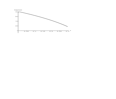
where $\Delta$ is defined between $0^{\circ}$ and $180^{\circ}$. The attached uncertainty comes from the experimental errors of the branching fractions, which are treated as uncorrelated here. Since we determine $\Delta$ through $\cos\Delta$ which is sensitive to small experimental errors near $\Delta=90^{\circ}$, the uncertainty in Eq.(17) turns out to be a little larger than one might expect from those of the branching fractions. One may wonder how much $\Delta$ can be reduced by adding the breaking term $A_{\gamma 8}$ with the constraint of Eq.(14). The result is plotted in Fig.1. Dependence of $\Delta$ on the ratio $r=A_{\gamma 8}/A_{\gamma}$ is very mild: $\Delta$ decreases slowly and monotonically from $90^{\circ}$ at $r=0$ to $58^{\circ}$ at the edge of the allowed range, $r=0.3$. Even if the FSI phases of $A_{\gamma}$ and $A_{\gamma 8}$ are left independent, it is fairly obvious that we cannot fit the data with small values for all phase differences under the constraint $F_{K}(m^{2}_{J/\psi})\geq F_{\pi}(m^{2}_{J/\psi})$. We have thus come to the conclusion that the FSI phase difference between the one-photon and the gluon decay amplitudes is very large, as large as $90^{\circ}$. For this magnitude, it must come mostly from the long-distance FSI.

V Perspectives

Our conclusion of large FSI phases has a profound implication in the $B$ decay. The important input leading to this conclusion is that the electromagnetic form factor of $K^{+}$ does not fall faster than that of $\pi^{+}$. While it is very reasonable in perturbative QCD, we can in principle test this postulate in experiment. Just measure the ratio of the one-photon annihilation cross sections for $e^{+}e^{-}\rightarrow\pi^{+}\pi^{-}$ and $K^{+}K^{-}$ off the $J/\psi$ peak. We do not have good data on the ratio $\sigma_{K^{+}K^{-}}/\sigma_{\pi^{+}\pi^{-}}$ off the peak. Experiment requires time and a good $\pi^{+}/K^{+}$ separation. A measurement will certainly have a great impact on the issue of the long-distance FSI in heavy particle decays. The magnitude of measured cross sections will also tell how close the form factors are to their asymptotic limits and therefore how small the phases of $A_{\gamma}$ and $A_{\gamma 8}$ are. Even a value of the unseparated ratio $\sigma_{K^{0}\overline{K}^{0}}/(\sigma_{K^{+}K^{-}}+\sigma_{\pi^{+}\pi^{-}})$ off the peak will throw in one more input in the analysis.

TABLE I.: The SU(3) parametrization of the $0^{-}0^{-}$ decay amplitudes of $J/\psi$ and their magnitudes from the observed decay branching fractions. The central value of the $\pi^{+}\pi^{-}$ amplitude is normalized to unity.

Decay modes	$\pi^{+}\pi^{-}$	$K^{+}K^{-}$	$K^{0}\overline{K}^{0}$
Parametrization	$\;\;\;A_{\gamma}-\sqrt{2/3}A_{8\gamma}$	$A_{8}+A_{\gamma}+\sqrt{2/3}A_{8\gamma}$	$A_{8}-\sqrt{2/3}A_{8\gamma}$
$|$Measured$|$	1.000$\pm$0.078	1.367$\pm$0.089	0.925$\pm$0.060

FIG. 1.: The relative phase $\Delta$ in degrees between $A_{8}$ and $A_{\gamma}$ as a function of real parameter $r=A_{\gamma 8}/A_{\gamma}$ in its allowed range. $\Delta$ is drawn between $0^{\circ}$ and $90^{\circ}$ since $\Delta\rightarrow 180^{\circ}-\Delta$ under the redefinition of $A_{\gamma}\rightarrow-A_{\gamma}$.