Charged Higgs and Scalar Couplings in Semileptonic Meson Decay

Abstract

We present a new charged Higgs search technique using the effects of scalar dynamics in semileptonic meson decay. Applying this method to a modest sample of $B$ meson decays yields sensitivity to the high $\tan{\beta}$ region well beyond existing charged Higgs searches.

RUTGERS-99-04

Department of Physics and Astronomy, Rutgers University
Piscataway, New Jersey 08855
tesarek@physics.rutgers.edu

Past searches for charged Higgs can be put into four categories: 1) direct production in colliders, 2) measurement of anomalously large branching ratios for top, bottom and $\tau$ lepton decays, 3) lepton polarization measurements in meson decay and 4) precision measurements of well known quantities such as $K^{0}$–$\overline{K^{0}}$ mixing, $Z$ width, etc. [1]. Category 1 represent direct searches while categories 2–4 are indirect search techniques. Of the indirect searches, only the lepton polarization technique makes use of the scalar nature of the charged Higgs. Requiring scalar dynamics in a process which may be mediated by a charged Higgs provides an extra constraint and narrows the number of possible interpretations of indirect searches.

In this Letter, we review a method to identify scalar dynamics or couplings in semileptonic decays of pseudoscalar mesons. By identifying the scalar coupling as a charged Higgs mediating the decay, one may extract the relative $H^{\pm}/W^{\pm}$ coupling strengths. We apply the relative coupling strength information to a two Higgs doublet model and evaluate the possible sensitivities of precision measurements in $B$ meson decay dynamics to charged Higgs searches.

General Phenomenology

We begin by considering a general semileptonic meson decay.

$$M\rightarrow m\ell\nu,$$ (1)

where $M$ and $m$ denote the parent and offspring pseudoscalar mesons and $\ell$ and $\nu$ refer to the charged lepton and its neutrino. The general amplitude describing a pseudoscalar to pseudoscalar transition, consistent with the Dirac equation and left handed, massless neutrinos, is

$$\begin{array}[]{cc}{\cal M}=&\frac{G_{F}}{\sqrt{2}}V_{ij}\overline{u}(p_{\nu})(1+\gamma^{5})\left\{Mf_{S}-\frac{1}{2}\left[(P+p)_{\alpha}f_{+}\right.\right.\\ &+\left.\left.(P-p)_{\alpha}f_{-}\right]\gamma^{\alpha}+i\frac{f_{T}}{M}\sigma_{\alpha\beta}P^{\alpha}p^{\beta}\right\}v(p_{\ell}),\end{array}$$ (2)

where $G_{F}$ is the Fermi coupling constant, $V_{ij}$ is the appropriate Cabibbo-Kobayashi-Maskawa [2] (CKM) matrix element and $P$, $M$ and $p$, $m$ are the 4-momenta and masses of the parent and offspring mesons, respectively. This transition amplitude contains four form factors, $f_{S}$, $f_{+}$, $f_{-}$, and $f_{T}$, which parameterize the $M\rightarrow m$ transition and provide a measure of the admixture of different dynamics or couplings occurring in the decay. In general, the form factors depend on the 4-momentum transferred to the leptons, $Q^{2}=(P-p)^{2}$. Two of the form factors, $f_{+}$ and $f_{-}$, arise from a vector particle mediating the decay while the remaining form factors, $f_{S}$ and $f_{T}$, come from scalar and tensor exchange. The term in equation 2 involving $f_{-}$ may be collapsed, using the Dirac equation, to give an induced scalar coupling. The tensor term may be similarly collapsed into induced vector and scalar components.

To calculate the decay rate, we use the notation of Chizhov [3] and define parameters for effective vector and scalar terms:

$$\begin{array}[]{ll}V=&f_{+}+\frac{m_{\ell}}{M}f_{T}\hfill\\ S=&f_{S}+\frac{m_{\ell}}{2M}f_{-}+\left\{\frac{(E_{\nu}-E_{\ell})}{M}+\frac{m_{\ell}^{2}}{2M^{2}}\right\}f_{T}.\end{array}$$ (3)

The decay rate can then be calculated in the rest frame of the parent meson.

$$\Gamma(E_{m},E_{\ell})\propto A\cdot|V|^{2}+B\cdot\Re(V^{*}S)+C\cdot|S|^{2},$$ (4)

where $A$, $B$ and $C$ depend on the kinematics of the decay.

$$A = M(2E_{\ell}E_{\nu}-M\Delta E_{m})-m_{\ell}^{2}\left(E_{\nu}-\frac{1}{4}\Delta E_{m}\right),$$

$$B = mM(2E_{\nu}-\Delta E_{m}),$$ (5)

$$C = M^{2}\Delta E_{m},$$

and

$$\Delta E_{m}=\frac{M^{2}+m^{2}-m_{\ell}^{2}}{2M}-E_{m}.$$ (6)

From equation 3, note that the induced scalar coupling is suppressed for heavy mesons decaying into light leptons by the factor $m_{\ell}/M$. This suppression factor limits the ability to search for scalar effects unless one has a priori knowledge of $f_{-}$. This limitation will be discussed when applying the general analysis to specific decays.

As an aside, we observe that the form factors may be complex with non-zero phases. While an overall phase is unobservable, the decay rate is sensitive to the relative phases of the form factors, $\phi_{ij}=\phi_{i}-\phi_{j},$ where $i$, $j$ denote the form factor indices: $+$, $-$, $S$ or $T$. The interference terms between the form factors then enter the decay rate as:

$$\Re{\{f_{i}^{*}f_{j}\}}=|f_{i}(Q^{2})||f_{j}(Q^{2})|\cos{\phi_{ij}}.$$ (7)

It is interesting to note that if $f_{+}$, $f_{-}$, $f_{S}$ and $f_{T}$ are not all relatively real ($\phi_{ij}=0,\pi$) then CP is violated.

The scalar and tensor coupling strengths may be isolated by reparameterizing these form factors as a product of a structure dependent term which depends on the momentum transfer, $F_{i}(Q^{2})$, and a relative coupling strength, $g_{i}$;

$$f_{i}(Q^{2})=F_{i}(Q^{2})g_{i},$$ (8)

where $i$ denotes either $S$ or $T$. In order to be sensitive to deviations from pure vector behavior, we remove a common factor of $f_{+}(0)$ from equation 2. Then, in the limit of no momentum transferred to the leptons ($Q^{2}=0$),

$$\left|\frac{f_{i}(0)}{f_{+}(0)}\right|=\frac{|F_{i}|}{|f_{+}|}g_{i},$$ (9)

where the explicit reference to the $Q^{2}$ dependence is dropped. For the remainder of this Letter, form factors will be assumed to be evaluated at $Q^{2}=0$. In order to extract the relative coupling strengths, $g_{i}$, from a form factor ratio, one need only know the ratio $|F_{i}/f_{+}|$. For tensor couplings, this ratio must be evaluated on a case-by-case basis. Note that in the heavy quark limit, $|f_{-}/f_{+}|=1$ [4]. Since the induced scalar is indistinguishable from a true scalar exchange, we argue that $|F_{S}/f_{+}|=1$.

Any two Lorentz invariants may be used to describe the phase space of a three body decay. For semileptonic decays, it is traditional to choose the kinetic energies of the offspring meson ($T_{m}=E_{m}-m_{m}$) and the lepton ($T_{\ell}=E_{\ell}-m_{\ell}$) where both energies are measured in the parent meson rest frame. Figure 1 shows how the different couplings affect the phase space density or Dalitz plot for $B^{0}\rightarrow D^{-}\mu^{+}\nu$ decay. The figure shows that the character of the Dalitz plot changes dramatically depending on the Lorentz structure of the coupling.

Analysis of the shape of the Dalitz plot for semileptonic decays would then yield information about possible tensor and scalar couplings. Non-zero values of either tensor or scalar couplings would indicate the onset of new types of physics not predicted by the Standard Model of particle physics. Tensor couplings have previously been discussed in the literature [5, 6] and are beyond the scope of this Letter. Scalar couplings have also been discussed in the context of charged Higgs exchange [6]. Outside of CP violating effects, most of the charged Higgs phenomenology is discussed in terms of heavy quark or $\tau$ decay [1] where the couplings are expected to be the strongest. However, from equation 4 the decays of mesons into relatively light ($m_{\ell}/M\ll 1$) leptons provide an interesting probe for scalar effects and may yield information on charged Higgs. In this context, we now evaluate charged Higgs couplings.

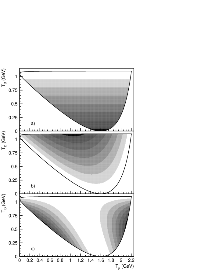
Figure 1: Phase space density contours for decays of $B^{0}\rightarrow D^{-}\mu^{+}\nu$ showing the effects of a) scalar, b) vector and c) tensor couplings in the decay. The variables plotted are the $D^{-}$ and $\mu^{+}$ kinetic energies $(T_{D},T_{\mu})$. Darker colors represent a higher phase space plot density.

Charged Higgs Couplings

In theories where multiple Higgs doublets are responsible for the spontaneous symmetry breaking of the electromagnetic and weak interactions, charged Higgs particles arise as a consequence of the theory. A charged Higgs particle may mediate semileptonic decays in the same manner as a $W^{\pm}$. The differences between $H^{\pm}$ and $W^{\pm}$ mediation arise from the Lorentz structure of the coupling and the coupling strength. In general, the Higgs-fermion coupling strengths are model dependent. We consider a type-II two Higgs doublet model where one Higgs doublet, $\phi_{2}$, couples to down-type quarks and charged leptons and the other Higgs doublet couples to up-type quarks. Minimal supersymmetry predicts a type-II Higgs model with added constraints. For a large charged Higgs mass ($M_{H^{\pm}}\gg M$) one may write down the Lagrangian density describing the Higgs-fermion interaction using the Fermi formalism. In terms of the ratio of vacuum expectation values $X=v_{2}/v_{1}\equiv\tan{\beta}$ and $Y=1/X\equiv\cot{\beta}$ the Lagrangian density for type-II Higgs models is [7]:

$${\cal L}_{H} = 2^{\frac{3}{4}}G_{F}^{\frac{1}{2}}H^{+}\left\{\overline{U}\left[XV_{ij}M_{D}(1+\gamma^{5})+YM_{U}V_{ij}(1-\gamma^{5})\right]D\right.$$ (10)

$$\left.+\overline{\nu}XM_{L}(1+\gamma^{5})L\right\}+{\rm h.c.},$$

where $M_{D}$, $M_{U}$ and $M_{L}$ are the diagonal mass matrices, and

$$U=\left(\begin{array}[]{c}u\\ c\\ t\end{array}\right),D=\left(\begin{array}[]{c}d\\ s\\ b\end{array}\right),\\ L=\left(\begin{array}[]{c}e\\ \mu\\ \tau\end{array}\right),\nu=\left(\begin{array}[]{c}\nu_{e}\\ \nu_{\mu}\\ \nu_{\tau}\end{array}\right).$$ (11)

For the theory to be perturbative regime and allow us to write and evaluate Feynman diagrams for the decay processes, the $H^{+}$–$t$, $H^{+}$–$b$ coupling strength must be small. This leads to two limiting conditions:

$$\begin{array}[]{ccc}X\ll 1,&\frac{G_{F}}{8\pi\sqrt{2}}m_{b}^{2}X^{2}&\ll 1,\\ X\gg 1,&\frac{G_{F}}{8\pi\sqrt{2}}m_{t}^{2}Y^{2}&\ll 1,\end{array}$$ (12)

which reduces to the range $0.20<X<200$.

The quark level transition amplitudes for the decay in equation 1 can then be written for mesons containing down-type quarks decaying into mesons containing up-type quarks (eg. $s\rightarrow u\ell\nu$, $b\rightarrow c\ell\nu$, etc).

$${\cal A}_{H} =i\frac{G_{F}}{\sqrt{2}}\frac{V_{ij}}{M_{H^{\pm}}^{2}}\left\{\overline{U}\left[Xm_{D}(1+\gamma^{5})+Ym_{U}(1-\gamma^{5})\right]D\right\}$$ (13)

$$\times\left\{\overline{\ell}Xm_{\ell}(1-\gamma^{5}){\nu}\right\},$$

where $m_{D}$ is the mass of the down-type quark ($s$, $b$) and $m_{U}$ is the mass of the up-type quark ($u$, $c$). For comparison, the transition amplitude for the weak interaction is

$${\cal A}_{W}=-i\frac{G_{F}}{\sqrt{2}}V_{ij}\left\{\overline{U}\gamma_{\mu}(1-\gamma^{5})D\right\}\left\{\overline{\ell}\gamma^{\mu}(1-\gamma^{5})\nu\right\}.$$ (14)

From the last two equations, one may read off the ratio of the Higgs coupling strength to the weak coupling strength.

$$g_{S}=\frac{G_{H^{\pm}}}{G_{Weak}}=\frac{m_{\ell}m_{D}}{M_{H^{\pm}}^{2}}X^{2}\left(1+\frac{m_{U}}{m_{D}}Y^{2}\right),$$ (15)

where $m_{D}$ and $m_{U}$ are the current masses of the appropriate up and down type quark, respectively and $|F_{s}/f_{+}|=1$.

The ratio, $g_{S}$, of the two couplings is the same $H^{\pm}$/$W^{\pm}$ coupling strength found in equation 9. A measurement of the relative size of the scalar and vector form factors, then gives a relationship between the Higgs mass and the ratio of vacuum expectation values in type-II two Higgs doublet models:

$$M_{H^{\pm}}=\left[\frac{m_{\ell}m_{D}}{g_{s}}\left(1+\frac{m_{U}}{m_{D}X^{2}}\right)\right]^{\frac{1}{2}}X.$$ (16)

We now consider the application of the above phenomenology to $B$ meson decays.

$B$ meson decays

In principle, one may fit the measured Dalitz plot of $B\rightarrow D\mu\nu$ decays for the relative admixture of the different form factors ($|f_{-}/f_{+}|$, $|f_{S}/f_{+}|$, $|f_{T}/f_{+}|$) and the relative phases of the form factors.

In practice, the situation is more challenging. In the discussion below, experience is derived from over two decades of kaon research in the literature. In $K\rightarrow\pi\ell\nu$ decays, the $Q^{2}$ dependence of the vector form factor has been shown to be linear [8], and is usually parameterized,

$$f_{+}(Q^{2})=f_{+}(0)\left(1+\lambda_{+}\frac{Q^{2}}{m_{\pi}^{2}}\right).$$ (17)

The values of $\lambda$ are small and may be approximated by a small change in slope of the phase space distribution in the $T_{\pi}$ direction. In the $T_{\pi}$ direction, the effect of the $Q^{2}$ dependence of the vector form factor is similar to introducing a small scalar coupling. When fitting the Dalitz plot, $\lambda_{+}$ is correlated with $|f_{S}/f_{+}|$. As a further complication, electromagnetic radiative effects are significant in some regions of phase space [9, 10]. If not taken into account, the net result produces a shift in the phase space distribution which would appear as an admixture of scalar and tensor couplings. These effects are expected to manifest themselves in B decays in much the same manner as in kaon decays.

Semileptonic B decays of the form $B\rightarrow D\mu\nu$ appear to have the most sensitivity to the effects described above. In addition to the advantages of a larger coupling as demonstrated by equation 15, using the muonic decays reduces electromagnetic radiative effects by approximately a factor of $m_{\mu}/m_{e}\approx 200$. Unfortunately, from equation 3, the suppression of the induced scalar term ($f_{-}$) for muonic decays is less than for electronic decays.

In order to estimate the sensitivity of this method using B decay, one may use the uncertainties from low statistics kaon results as a guide. With a sample of 2500 exclusive $B\rightarrow D\mu\nu$ decays one would expect an induced scalar contribution of $f_{-}=0.02$ and an error on $|f_{S}/f_{+}|\approx 0.04$. Based on these numbers one would expect an experimental sensitivity in the large $\tan{\beta}$ region of

$$M_{H^{\pm}}<2.44\tan{\beta}\;\rm GeV/c^{2}\;(95\%CL).$$ (18)

In this calculation, we assume a $b$ quark mass of $4.4\;\rm GeV/c^{2}$. Figure 2 compares the expected experimental charged Higgs sensitivity in the $M_{H^{\pm}}$ vs $\tan{\beta}$ plane using the method described above with current experimental results from direct searches [11, 12]. This method of indirect Higgs search shows significant sensitivity well beyond existing experimental data. However, further increase of the sensitivity shown in the Figure by increasing the available statistics is likely not possible due to the induced scalar effects.

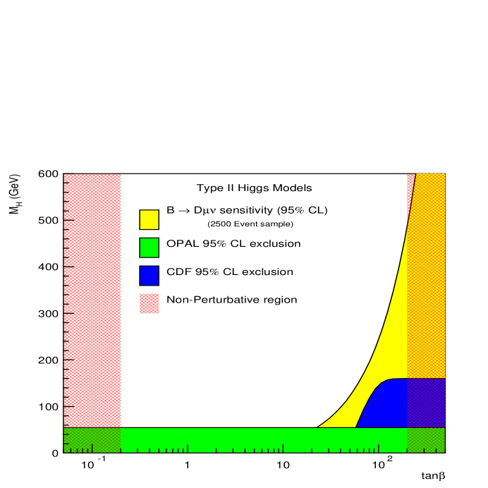
Figure 2: Charged Higgs 95% exclusion curves in the $(M_{H^{\pm}},\tan{\beta})$ plane for $B\rightarrow D\mu\nu$ decays. The CDF and OPAL results are from direct searches.

Other indirect searches from the decays of $B$ mesons have set limits on the charged Higgs [13, 14]. The most restrictive of these searches comes from the CLEO measurement of BR($b\rightarrow s\gamma$) which gives an exclusion of $M_{H^{\pm}}>[244+63/(\tan{\beta})^{1.3}]$ GeV [13]. Measuring the couplings as described above has sensitivity in the high, $80<\tan{\beta}<200$ region. Probably more important, since the above method measures the coupling to the hadronic current, penguin diagrams do not contribute to a scalar Lorentz structure. Thus the above charged Higgs search technique can illuminate a portion of the charged Higgs parameter space not yet explored in a way that is less model dependent.

Summary

Potential discovery of charged Higgs from direct production in $e^{+}e^{-}$ machines are limited by the beam energy (100 GeV for LEP). At the Tevatron, direct searches are currently limited by top production and the top mass [11]. The direct searches are unlikely to exceed these limits in the near future. Therefore it becomes necessary to consider indirect methods for charged Higgs searches.

Using a traditional Dalitz plot analysis for $B$ meson decay, we have shown sensitivity to the effects of charged Higgs. Based on coarse estimates of the measurement uncertainties, we estimate that this technique is sensitive to charged Higgs in regions of the $M_{H^{\pm}}$ vs $\tan{\beta}$ parameter space previously unexplored. Further, this method is sensitive to regions of parameter space inaccessible to direct searches in existing colliders.

The author acknowledges support from the National Science Foundation under grant NSFPHY97-25210. We also thank G. Farrar, N. Polonsky and S. Schnetzer for useful discussions and critical comments.

References

- [1] J.L. Hewett, S. Thomas, T. Takeuchi, “Indirect Probes of New Physics” Published in Electroweak Symmetry Breaking and New Physics at the TeV Scale. Ed. T.L. Barklow, S. Dawson, H.E. Haber, J. L Siegist, World Scientific Publishing Co. (1996).
- [2] N. Cabibbo, Phys. Rev. Lett. 10, (1963) 531; M. Kobayashi and T. Maskawa, Prog. Theor. Phys. 49, (1973) 652.
- [3] M.V. Chizhov, eprint hep-ph/9511287 (1995).
- [4] N. Isgur and M.B. Wise, Phys. Lett. B237, (1990) 527; Phys. Lett., B232, (1989) 113.
-
[5]
C.Q. Geng and S.K. Lee, Phys. Rev. D51, (1996) 99;
M.V. Chizhov, Mod. Phys. Lett. A8, (1993) 2753;
N.V. Bolotov, et al., Phys. Lett. B243, (1990) 308. - [6] A.A. Poblaguev, Phys. Lett. B238, (1990) 108; Phys. Lett. B286, (1992) 169.
-
[7]
S. Glashow and S. Weinberg, Phys. Rev. D15, (1977) 1958;
J.F. Donoughue and L.F. Li, Phys. Rev. D19, (1979) 945. - [8] Particle Data Group (C.Caso, et al.,) Eur. Phys. Jour. C3, (1998).
- [9] E.S. Ginsberg. Phys. Rev. 171, (1968) 1675; E.S. Ginsberg. Phys. Rev. 175, (1968) 2169; H.W. Fearing, E. Fischbach, J. Smith. Phys. Rev. D2, (1970) 542; B.R. Holstein. Phys. Rev. D41, (1990) 2829.
- [10] E.S. Ginsberg, J. Smith. Phys. Rev. D8, (1973) 3887.
-
[11]
F. Abe, et al., Phys. Rev. Lett. 79, (1997) 357;
F. Abe, et al., Phys. Rev. Lett. 72, (1994) 1977. - [12] G. Abbiendi, et al., eprint hep-ex/9811025.
- [13] M.S. Alam, et al., Phys. Rev. Lett. 74, (1995) 2885.
-
[14]
M. Acciarri, et al., Phys. Lett. B396, (1997) 327;
D. Buskulic, et al., Phys. Lett. B343, (1995) 444.