Is there a light fermiophobic Higgs ?

Abstract

The most general Two Higgs Doublet Model potential without explicit CP violation depends on 10 real independent parameters. There are two different ways of restricting this potential to 7 independent parameters. This gives rise to two different potentials, $V_{(A)}$ and $V_{(B)}$. The phenomenology of the two models is different, because some trilinear and quartic Higgs couplings are different. As an illustration, we calculate the decay width of $h^{0}\rightarrow\gamma\gamma$, where precisely due to the different trilinear couplings the loop of the charged Higgs gives different contributions. We also discuss the possibility for the existence of a light fermiophobic Higgs.

I Introduction

Despite the great success of the standard $SU(2)\times U(1)$ electroweak model (SM), one of its fundamental principles, the spontaneous symmetry breaking mechanism, still awaits experimental confirmation. This mechanism, in its minimal version, requires the introduction of a single doublet of scalar complex fields and gives rise to the existence of a neutral particle with mass $m_{H}$. The combined analysis [1] of all electroweak data as a function of $m_{H}$ favors a value of $m_{H}$ close to $100\;GeV/c^{2}$ and predicts with 95% confidence level an upper bound of $m_{H}<200\;GeV/c^{2}$. Hence, one can still envisage the possibility of a Higgs discovery in the closing stages of the LEP operation.

Nevertheless, even if this turned out to be true, one still would like to know if there is just one family of Higgs fields or, on the contrary, if nature has decided to replicate itself. In our view this is the main motivation to consider multi Higgs models. In this paper we continue the study of the two-Higgs-doublet model (2HDM). Following our previous work [2], we examine models without explicit CP violation and which are also naturally protected from developing a spontaneous CP breaking minimum. There are two different ways of achieving this. To illustrate the different phenomenology we calculate, in both models, the decay width for the process $h^{0}\rightarrow\gamma\gamma$, which can be particularly relevant if $h^{0}$ is a fermiophobic Higgs.

II The potentials

The Higgs mechanism in its minimal version (one scalar doublet) introduces in the theory an arbitrary parameter — the Higgs boson mass $m_{H}$. In fact, the potential depends on two parameters, which are the coefficients of the quadratic and quartic terms. However the perturbative version of the theory replaces them by the vacuum expectation value $v=247\;GeV$ and by $m_{H}$. If we generalize the theory introducing a second doublet of complex fields, the number of free parameters in the potential $V$ grows from two to fourteen. At the same time, the number of scalar particles grows from one to four. In this general form the potential contains genuine new interaction vertices which are independent of the vacuum expectation values and of the mass matrix of the Higgs bosons. However, these new interactions can be avoided if one imposes the restriction that $V$ is invariant under charge conjugation $C$. In fact, if $\Phi_{i}$ with $i=1,2$ denote two complex scalar doublets with hyper-charge 1, under $C$ the fields transform themselves as $\Phi_{i}\rightarrow\exp(i\alpha_{i})\Phi_{i}^{*}$ where the parameters $\alpha_{i}$ are arbitrary. Then, choosing $\alpha_{1}=\alpha_{2}=0$, and defining $x_{1}=\phi_{1}^{\dagger}\phi_{1}$, $x_{2}=\phi_{2}^{\dagger}\phi_{2}$, $x_{3}=\Re\{\phi_{1}^{\dagger}\phi_{2}\}$ and $x_{4}=\Im\{\phi_{1}^{\dagger}\phi_{2}\}$ it is easy to see that the most general 2HDM potential without explicit $C$ violation, is:

$$V=-\mu_{1}^{2}x_{1}-\mu_{2}^{2}x_{2}-\mu_{12}^{2}x_{3}+\lambda_{1}x_{1}^{2}+\lambda_{2}x_{2}^{2}+\lambda_{3}x_{3}^{2}+\lambda_{4}x_{4}^{2}+\lambda_{5}x_{1}x_{2}+\lambda_{6}x_{1}x_{3}+\lambda_{7}x_{2}x_{3}\enskip.$$ (1)

In general, the minimum of this potential is of the form

$$\left<\Phi_{1}\right> = \frac{1}{\sqrt{2}}\left(\begin{array}[]{l}0\\ v_{1}\end{array}\right)$$ (2c)

$$\left<\Phi_{2}\right> = \frac{1}{\sqrt{2}}\left(\begin{array}[]{l}0\\ v_{2}e^{i\theta}\end{array}\right)\quad,$$ (2f)

in other words it breaks $CP$ spontaneously. To use this potential in perturbative electroweak calculations the physical parameters that should replace the $\lambda$’s and $\mu$’s are the following:

1. the position of the minimum, $v_{1}$, $v_{2}$ and $\theta$, or alternatively, $v^{2}=v_{1}^{2}+v_{2}^{2}$, $\tan\beta=\frac{v_{2}}{v_{1}}$ and $\theta$;

2. the masses of the charged boson $m_{+}$ and of the three neutral bosons $m_{1}$, $m_{2}$ and $m_{3}$;

3. and the three Cabibbo like angles $\alpha_{1}$, $\alpha_{2}$ and $\alpha_{3}$ that represent the orthogonal transformation that diagonalizes the $3\times 3$ mass matrix of the neutral sector.

In a previous paper[2] we have examined the different types of extrema for potential $V$. In particular it was shown in [2] that there are two ways of naturally imposing that a minimum with $CP$ violation never occurs. This, in turn, leads to two different 7-parameter potentials. The first one, denoted $V_{(A)}$, is the potential discussed in the review article of M. Sher[3] and corresponds to setting $\mu_{12}^{2}=\lambda_{6}=\lambda_{7}=0$ in equation (1). The second 7-parameter potential, that we shall call $V_{(B)}$, is essentially the version analyzed in the Higgs Hunters Guide[4] and it corresponds to the conditions $\lambda_{6}=\lambda_{7}=0$ and $\lambda_{3}=\lambda_{4}$. As we have already pointed out [2] but would like to stress again, these potentials have different phenomenology. This is illustrated in section III when we consider the fermiophobic limit of both models.

Since $V_{(A)}$ and $V_{(B)}$ do not have spontaneous $CP$-violation, the number of so-called “physical parameters” is immediately reduced to seven. In fact, $\theta=0$ and only one rotation angle, $\alpha$, is needed to diagonalize the $2\times 2$ mass matrix of the $CP$-even neutral scalars. This is clearly seen if we transform the initial doublets $\Phi_{i}$ into two new ones $H_{i}$ given by

$$\left(\begin{array}[]{c}H_{1}\\ H_{2}\end{array}\right)=\frac{1}{\sqrt{v_{1}^{2}+v_{2}^{2}}}\left(\begin{array}[]{rr}v_{1}&v_{2}\\ -v_{2}&v_{1}\end{array}\right)\left(\begin{array}[]{c}\Phi_{1}\\ \Phi_{2}\end{array}\right)\quad.$$ (3)

In this Higgs bases, only $H_{1}$ acquires a vacuum expectation value. Then, the $T_{3}=+\frac{1}{2}$ component and the imaginary part of the $T_{3}=-\frac{1}{2}$ component of $H_{1}$ are the $W^{\pm}$ and $Z$ would be Goldstone bosons, respectively. The $C$-odd neutral boson, $A^{0}$, is the imaginary part of the $T_{3}=-\frac{1}{2}$ component of $H_{2}$. On the other hand, the light and heavy $CP$-even neutral Higgs, $h^{0}$ and $H^{0}$, are linear combinations of the real parts of the $T_{3}=-\frac{1}{2}$ component of $H_{1}$ and $H_{2}$.

Notice that $V_{(A)}$ is invariant under the $Z_{2}$ transformation $\Phi_{1}\rightarrow\Phi_{1}$ and $\Phi_{2}\rightarrow-\Phi_{2}$, whereas in $V_{(B)}$ only the $\mu_{12}^{2}$ term breaks the $U(1)$ symmetry, $\Phi_{2}\rightarrow e^{i\alpha}\Phi_{2}$. Because this breaking occurs in a quadratic term it does not spoil the renormalizability of the model. Hence, in both cases the terms that were set explicitly to zero, will not be needed to absorb infinities that occur at higher orders. The complete renormalization program of the model based on $V_{(A)}$ was carried out in [5]. The results for $V_{(B)}$ are similar but the cubic and quartic scalar vertices have to be changed appropriately.

For the sake of completeness we will close this section with a summary of the results that will be used later. As we have already said they are not new and can be obtained either from [3] or [4]. We agree with both.

For $V_{(A)}$ the minimum conditions are

$$0\quad=\quad T_{1} = v_{{1}}\left(\,-\mu_{{1}}^{2}+\lambda_{{1}}{v_{{1}}}^{2}+\lambda_{+}\,{v_{{2}}}^{2}\right)$$ (4a)

$$0\quad=\quad T_{2} = v_{{2}}\left(\,-\mu_{{2}}^{2}+\lambda_{{2}}{v_{{2}}}^{2}+\lambda_{{+}}\,{v_{{1}}}^{2}\right)$$ (4b)

with $\lambda_{+}=\frac{1}{2}(\lambda_{3}+\lambda_{5})$. They lead to the following solutions:
either i)

$$v_{1}^{2} = \frac{\lambda_{2}\mu_{1}^{2}-\lambda_{+}\mu_{2}^{2}}{\lambda_{1}\lambda_{2}-\lambda_{+}^{2}}$$ (5a)

$$v_{2}^{2} = \frac{\lambda_{1}\mu_{2}^{2}-\lambda_{+}\mu_{1}^{2}}{\lambda_{1}\lambda_{2}-\lambda_{+}^{2}}\quad;$$ (5b)

oreth ii)

$$v_{1}^{2} = 0$$ (6a)

$$v_{2}^{2} = \frac{\mu_{2}^{2}}{\lambda_{2}}\quad.$$ (6b)

The masses of the Higgs bosons and the angle $\alpha$ are given by the following relations:

$$m_{H^{+}}^{2} = -\lambda_{3}\,\left(v_{1}^{2}+v_{2}^{2}\right)$$ (7a)

$$m_{A^{0}}^{2} = \frac{1}{2}\left(\lambda_{4}-\lambda_{3}\right)\,\left(v_{1}^{2}+v_{2}^{2}\right)$$ (7b)

$$m_{H^{0},h^{0}}^{2} = \lambda_{1}v_{1}^{2}+\lambda_{2}v_{2}^{2}\,\pm\,\sqrt{\left(\lambda_{1}v_{1}^{2}-\lambda_{2}v_{2}^{2}\right)^{2}+v_{1}^{2}v_{2}^{2}(\lambda_{3}+\lambda_{5})^{2}}$$ (7c)

$$\tan 2\alpha=\frac{v_{2}v_{1}\,(\lambda_{3}+\lambda_{5})}{\lambda_{1}v_{1}^{2}-\lambda_{2}v_{2}^{2}}\qquad.\qquad\qquad\qquad\qquad\qquad\qquad\quad$$ (8)

On the other hand, for $V_{(B)}$ the minimum conditions are

$$0 = T_{1}-\frac{\mu_{12}^{2}}{2}\,v_{2}$$ (9a)

$$0 = T_{2}-\frac{\mu_{12}^{2}}{2}\,v_{1}$$ (9b)

with the $T_{i}$ given by the previous equations (4). The solution of this set of equations is

$$v_{1}^{2} = \frac{\lambda_{1}-\lambda_{2}\pm\sqrt{\left(\lambda_{1}-\lambda_{2}\right)^{2}-4\left(\lambda_{1}-\lambda_{+}\right)\left(\lambda_{2}-\lambda_{+}\right)\left[\left(\lambda_{+}v^{2}-\mu_{1}^{2}\right)\left(\lambda_{2}v^{2}-\mu_{2}^{2}\right)-\mbox{$\frac{1}{4}$}\mu_{12}^{4}\right]}}{2\,\left(\lambda_{1}-\lambda_{+}\right)\left(\lambda_{2}-\lambda_{+}\right)}$$ (10a)

$$v_{2}^{2} = \frac{\lambda_{2}-\lambda_{1}\pm\sqrt{\left(\lambda_{1}-\lambda_{2}\right)^{2}-4\left(\lambda_{2}-\lambda_{+}\right)\left(\lambda_{1}-\lambda_{+}\right)\left[\left(\lambda_{+}v^{2}-\mu_{2}^{2}\right)\left(\lambda_{1}v^{2}-\mu_{1}^{2}\right)-\mbox{$\frac{1}{4}$}\mu_{12}^{4}\right]}}{2\,\left(\lambda_{1}-\lambda_{+}\right)\left(\lambda_{2}-\lambda_{+}\right)}\quad.$$ (10b)

Notice that, in this case, the solution with vanishing vacuum expectation value in one of the doublets is not possible. Now the masses and the value of $\alpha$ are given by

$$m_{H^{+}}^{2} = -\lambda_{3}\,\left(v_{1}^{2}+v_{2}^{2}\right)+\mu_{12}^{2}\,\frac{v_{1}^{2}+v_{2}^{2}}{v_{1}v_{2}}$$ (11a)

$$m_{A^{0}}^{2} = \frac{1}{2}\mu_{12}^{2}\,\frac{v_{1}^{2}+v_{2}^{2}}{v_{1}v_{2}}$$ (11b)

$$m_{H^{0},h^{0}}^{2} = \lambda_{1}v_{1}^{2}+\lambda_{2}v_{2}^{2}+\mbox{$\frac{1}{4}$}\mu_{12}^{2}\left(\mbox{$\frac{v_{2}}{v_{1}}$}+\mbox{$\frac{v_{1}}{v_{2}}$}\right)\,$$ (11d)

$$\pm\,\sqrt{\left(\lambda_{1}v_{1}^{2}-\lambda_{2}v_{2}^{2}+\mbox{$\frac{1}{4}$}\mu_{12}^{2}\left(\mbox{$\frac{v_{2}}{v_{1}}$}-\mbox{$\frac{v_{1}}{v_{2}}$}\right)\right)^{2}+\left(v_{1}v_{2}(\lambda_{3}+\lambda_{5})-\mbox{$\frac{1}{2}$}\mu_{12}^{2}\right)^{2}}$$

$$\tan 2\alpha=\frac{2\,v_{1}v_{2}\,\lambda_{+}-\mbox{$\frac{1}{2}$}\mu_{12}^{2}}{\lambda_{1}v_{1}^{2}-\lambda_{2}v_{2}^{2}+\mbox{$\frac{1}{4}$}\mu_{12}^{2}\left(\mbox{$\frac{v_{2}}{v_{1}}$}-\mbox{$\frac{v_{1}}{v_{2}}$}\right)}\qquad.\qquad\qquad\qquad\qquad\qquad$$ (12)

III The fermiophobic limit

Despite the fact that $V_{(A)}$ and $V_{(B)}$ are different, it is obvious that the gauge bosons and the fermions couplings to the scalars are the same for both models. In particular, the introduction of the Yukawa couplings without tree-level flavor changing neutral currents is easily done extending the $Z_{2}$ symmetry to the fermions. This leads to two different ways of coupling the quarks and two different ways of introducing the leptons, giving a total of four different models, usually denoted as model I, II, III and IV (cf. e.g. [5]).

In here, we use model I, where only $\Phi_{2}$ couples to the fermions. Then, the coupling of the lightest scalar Higgs, $h^{0}$, to a fermion pair (quark or lepton) is proportional to $\cos\alpha$. As $\alpha$ approaches $\frac{\pi}{2}$ this coupling tends to zero and in the limit it vanishes, giving rise to a fermiophobic Higgs.

Examining equations (8) and (12) we see that the fermiophobic limit ($\alpha=\frac{\pi}{2}$) can be obtained in potential A in two ways: either $\lambda_{+}=0$ or $v_{1}=0$. In potential B there is only one possibility $2v_{1}v_{2}\lambda_{+}=\frac{1}{2}\mu_{12}^{2}$. In this latter case, equations (11) and (12) give immediately:

$$m_{A^{0}}^{2} = 2\,\lambda_{+}\,\left(v_{1}^{2}+v_{2}^{2}\right)$$ (13a)

$$m_{H^{0}}^{2} = 2\,\lambda_{2}v_{2}^{2}\,+\,2\,\lambda_{+}v_{1}^{2}\quad=\quad m_{A^{0}}^{2}\,+\,2(\lambda_{2}-\lambda_{+})\,v^{2}\sin^{2}\beta$$ (13b)

$$m_{h^{0}}^{2} = 2\,\lambda_{1}v_{1}^{2}\,+\,2\,\lambda_{+}v_{2}^{2}\quad=\quad m_{A^{0}}^{2}\,-\,2(\lambda_{+}-\lambda_{1})\,v^{2}\cos^{2}\beta\quad.$$ (13c)

In the former case ($V_{(A)}$), $\lambda_{+}=0$ gives

$$m_{H^{0}}^{2} = 2\,\lambda_{2}v_{2}^{2}$$ (14a)

$$m_{h^{0}}^{2} = 2\,\lambda_{1}v_{1}^{2}$$ (14b)

while $v_{1}=0$ gives a massless $h^{0}$. In this analysis we have assumed that $v_{1}<v_{2}$. The reversed situation leads to similar conclusions since one is then interchanging the role of the two doublets.

The triple couplings involving two gauge bosons and a scalar particle like, for instance $Z_{\mu}Z^{\mu}h^{0}$, are always proportional to the angle $\delta=\alpha-\beta$. In particular, the couplings for $h^{0}$ are proportional to $\sin\delta$ whereas the corresponding $H^{0}$ couplings are proportional to $\cos\delta$. This general results can be understood if one recalls the argument about the role played by the neutral scalars in restoring the unitarity in the scattering of longitudinal $W$’s, i.e. in $W^{+}_{L}W^{-}_{L}\rightarrow W^{+}_{L}W^{-}_{L}$. The restoration of unitarity requires that the sum of the squares of the $W^{+}W^{-}h^{0}$ and $W^{+}W^{-}H^{0}$ couplings adds up to a constant proportional to the $SU(2)$ gauge coupling, $g$.

Current searches of the SM Higgs boson at LEP put the mass limit at $89\;GeV/c^{2}$[6]. Since the production mechanism is the reaction $e^{+}e^{-}\rightarrow Z^{*}\rightarrow Zh^{0}$, this limit can be substantially lower in the 2HDM if $\sin\delta$ is small. In our numerical application to the two $\gamma$ decay of a light fermiophobic $h^{0}$ we will explore the region $\sin^{2}\delta\leq 0.1$ [7].

Bounds on the Higgs masses have been derived by several authors [8]. Recently next-to-leading order calculations [9] in the SM give a prediction for the branching ratio $Br(B\rightarrow X_{s}\gamma)$ which is slightly larger than the experimental CLEO measurement[10]. In model II the charged Higgs loops always increase the SM value. Hence, this process provides good lower bounds on $m_{H^{\pm}}$ as a function of $\tan\beta$[9]. On the contrary, in model I the contribution from the charged Higgs reduces the theoretical prediction and so brings it to a value closer to the experimental result. This reduction is larger for small $\tan\beta$, since in model I the $H^{+}$ coupling to quarks is proportional to $\tan^{-1}\beta$. However, a small $\tan\beta$ gives a large top Yukawa coupling which leads to large new contributions to $R_{b}$, the $B_{0}-\bar{B}_{0}$ mixing. A recent analysis by Ciuchini et al. [9] derives the bounds $\tan\beta>1.8,\ 1.4\mbox{ and }1.0$ for $m_{H^{\pm}}=85,\ 200\mbox{ and }425\;GeV/c^{2}$, respectively.

The Higgs contribution to the $\rho$-parameter is [11]:

$$\Delta\rho=\frac{1}{16\pi^{2}v^{2}}\left[\sin^{2}\delta\;F(m_{H^{\pm}}^{2},m_{A^{0}}^{2},m_{H^{0}}^{2})\,+\,\cos^{2}\delta\;F(m_{H^{\pm}}^{2},m_{A^{0}}^{2},m_{h^{0}}^{2})\right]$$ (15)

where

$\displaystyle F(a,b,c)=a\,+\,\frac{bc}{b-c}\ln\frac{b}{c}\,-\,\frac{ab}{a-b}\ln\frac{a}{b}\,-\,\frac{ac}{a-c}\ln\frac{a}{c}\quad.$

Since the current experimental value of $\rho=1.0012\pm 0.0013\pm 0.0018$ [12] exceeds the SM prediction by 3$\sigma$, one should at least try to avoid a positive $\Delta\rho$.. A simpler examination of the function $F(a,b,c)$ shows that this is impossible if $m_{H^{\pm}}$ is the largest mass. On the other hand, if $m_{A^{0}}>m_{H^{\pm}}$ one obtains a negative value for $\Delta\rho$ which grows with the splitting $m_{A^{0}}-m_{H^{\pm}}$. In line with our limit ($\sin^{2}\delta\leq 0.1$), negative values of $\Delta\rho$ of the order of the experimental statistical error, i.e. $\Delta\rho\approx-10^{-3}$, can be obtained essentially in two ways. Either with a large $m_{H^{\pm}}\approx 300\;GeV/c^{2}$ but with a modest $m_{A^{0}}-m_{H^{\pm}}$ splitting ($m_{A^{0}}\approx 340\;GeV/c^{2}$) or with a smaller $m_{H^{\pm}}\approx 100\;GeV/c^{2}$ but with $m_{A^{0}}\approx 200\;GeV/c^{2}$. The variation of $\Delta\rho$ with $m_{h^{0}}$ is rather modest, less than $10$% for the range $20\;GeV/c^{2}\leq m_{h^{0}}\leq 100\;GeV/c^{2}$. With seven parameters in the Higgs sector it is difficult and not very illuminating to discuss in detail all possibilities. So, this discussion should be regarded as a simple justification for the fact that a fermiophobic Higgs scenario is not ruled out by the existing experiments. We would like to stress, that there could exist a light $h^{0}$ almost decoupled from the fermions ($\alpha\approx\frac{\pi}{2}$) and at the same time with a small LEP production rate via the $Z$-bremsstrahlungs reaction $Z^{*}\rightarrow Zh^{0}\;(\sin^{2}\delta\approx 10^{-1})$. If such a boson exists it will decay mainly via the process $h^{0}\rightarrow\gamma\gamma$.

IV The decay $\mbox{$h^{0}$}\longrightarrow\gamma\gamma$

The decay $\mbox{$h^{0}$}\rightarrow\gamma\gamma$ is particularly suitable to illustrate the fact that $V_{(A)}$ and $V_{(B)}$ give rise to different phenomenologies. In fact, the decay occurs at one-loop level and for a fermiophobic Higgs one has vector bosons and charged Higgs contributions. The latter are different for models $A$ and $B$, because the $h^{0}H^{+}H^{-}$ vertex is different. It is interesting to point out how this difference arises. Since the term in $\lambda_{4}$ does not contribute to this vertex, both potentials give rise to the same effective $h^{0}H^{+}H^{-}$ coupling, $g_{h^{0}H^{+}H^{-}}$, namely:

$$[h^{0}H^{+}H^{-}] = 2\,v_{2}\lambda_{2}\cos^{2}\beta\cos\alpha+v_{2}\lambda_{3}\sin\alpha\cos\beta\sin\beta-v_{1}\lambda_{5}\cos^{2}\beta\sin\alpha$$ (17)

$$-2\,v_{1}\lambda_{1}\sin^{2}\beta\sin\alpha+v_{2}\lambda_{5}\sin^{2}\beta\cos\alpha-v_{1}\lambda_{3}\cos\alpha\cos\beta\sin\beta$$

However, as we have already said, what is relevant for perturbative calculations is the position of the minimum of $V$ and the values of its derivatives at that point. This means that one has to express all coupling constants in terms of the particle masses. This is simply done by inverting equations (7) and (11). The result is

$$[h^{0}H^{+}H^{-}]_{(A)}=\frac{g}{m_{W}}\left(m_{h^{0}}^{2}\frac{\cos\left(\alpha\!+\!\beta\right)}{\sin 2\beta}-\left(m_{H^{+}}^{2}-\mbox{$\frac{1}{2}$}m_{h^{0}}^{2}\right)\sin\left(\alpha\!-\!\beta\right)\,\right)$$ (18)

and

$$[h^{0}H^{+}H^{-}]_{(B)}=\frac{g}{m_{W}}\left(\left(m_{h^{0}}^{2}-m_{A^{0}}^{2}\right)\frac{\cos\left(\alpha\!+\!\beta\right)}{\sin 2\beta}-\left(m_{H^{+}}^{2}-\mbox{$\frac{1}{2}$}m_{h^{0}}^{2}\right)\sin\left(\alpha\!-\!\beta\right)\,\right)$$ (19)

which clearly shows the difference that we have pointed out.

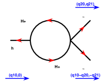
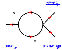
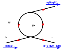
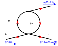
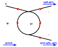
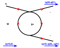
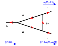
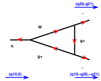
FIG. 1.: The contributing graphs to $h^{0}\rightarrow\gamma\gamma$ in the fermiophobic limit.

In Fig. 1 we show all the diagrams that were included. A previous work by Diaz and Weiler [14] did not include the Higgs-bosons diagrams. Our calculation, in the ’tHooft-Feynman gauge, was done with xloops[15, 16]. We have been using this program to calculate other amplitudes in the framework of the 2HDM [17]. Throughout this process we have made several checks on the computer results. In this particular case we have verified that the contribution of the vector boson loops agrees with a calculation done by M. Spira et al. [18] using the supersymmetric version of the 2HDM.

In Fig. 2 we show the product $m_{h^{0}}$ times the decay width ($\Gamma$) for the process $h^{0}\rightarrow\gamma\gamma$ in model A as a function of $\delta$ and for several values of $m_{h^{0}}$ and a fixed value of $m_{H^{+}}$. This function shows a gentle rise with $m_{h^{0}}$ which reflects the proportionality between $g_{h^{0}H^{+}H^{-}}$ and $m_{h^{0}}^{2}$. Looking at this coupling constant one could naively assume that there would be an enhancement for $\beta$ approaching $\pi/2$, i. e., in our plot, when $\delta$ approaches zero. However, a close examination shows that such an enhancement does not exist. On the contrary, the coupling vanishes in this limit, since $m_{h^{0}}$ goes to zero when $\beta\rightarrow\pi/2$. Alternatively, if one keeps $m_{h^{0}}$ fixed, then the mass relation

$$m_{h^{0}}=\sqrt{2\lambda_{1}}v_{1}=\sqrt{2\lambda_{1}}v\cos\beta$$ (20)

imposes a lower bound for $\beta$. In Fig. 2 the dotted line gives this limit, evaluated assuming $\lambda_{1}=1/2$. The dashed area shows the exclusion region implied by the LEP experimental results. In the work of Ackerstaff et al. [19] an experimental bound on the SM $h\rightarrow\gamma\gamma$ branching ratio is derived. For a fermiophobic Higgs with $m_{h}<m_{W}$ the $\gamma\gamma$ branching ratio is one. On the other hand, the production mechanism is suppressed by a factor $\sin^{2}\delta$. Hence, we have turned the OPAL experimental bounds into a bound on $\delta$. Fig. 3 gives the equivalent information for potential B.

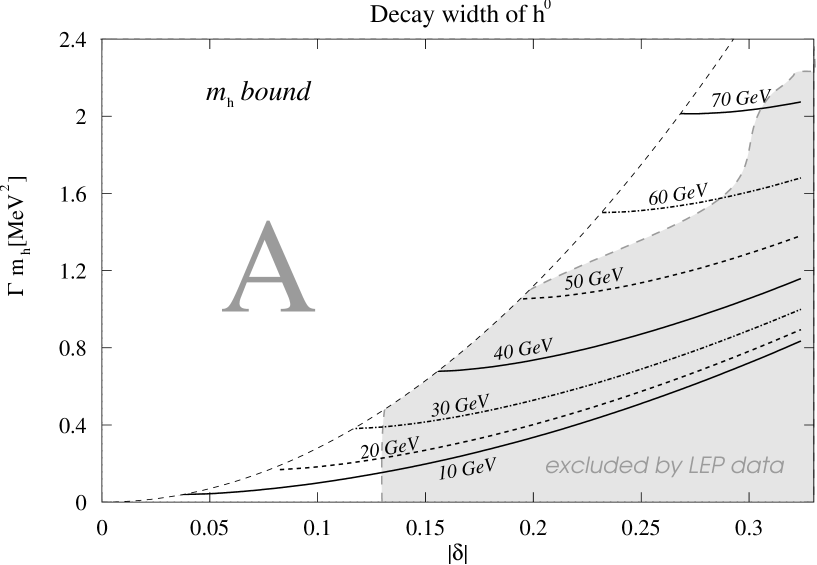
FIG. 2.: Dependence on $\delta$ and $m_{h^{0}}$ at $m_{H^{+}}=131\;GeV$ and $\alpha=\frac{\pi}{2}$ in potential A.

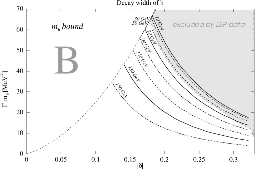
FIG. 3.: Dependence on $\delta$ and $m_{h^{0}}$ at $m_{H^{+}}=131\;GeV$ and $\alpha=\frac{\pi}{2}$ in potential B.

In Fig. 4 we plot, as a function of $m_{h^{0}}$, the ratio $R$, of the widthes calculated with potentials $V_{B}$ and $V_{A}$, respectively. According to the fermiophobic limit, we set $\alpha=\pi/2$ and $\delta=0.29$. For the other relevant masses we have used $m_{H^{+}}=200\;GeV/c^{2}$ and $m_{A^{0}}=250\;GeV/c^{2}$. In the range of variation of $m_{h^{0}}$, i.e., $20\;GeV/c^{2}<m_{h^{0}}<120\;GeV/c^{2}$, R decreases smoothly from 25 till 3. However, it is misleading to assume that potential A always gives smaller results. This is clearly shown in Fig. 5 where we plot the same function $R$ evaluated with the same parameters except for $m_{A^{0}}$ that was set up to $120\;GeV/c^{2}$. Again, $R$ is a decreasing function of $m_{h^{0}}$ that has a zero for $m_{h^{0}}$ around $70\;GeV/c^{2}$ and increases afterwards. However, in this case, the values obtained with potential B are smaller than the corresponding ones for potential A.

FIG. 4.: Ratio of the decay widthes from $V_{(B)}/V_{(A)}$ with $\delta=0.29$ and $m_{H^{+}}=200\;GeV$ and $m_{A^{0}}=250\;GeV$.

This behavior can be qualitatively understood if one examines the coupling constants $[h^{0}H^{+}H^{-}]_{(A)}$ and $[h^{0}H^{+}H^{-}]_{(B)}$ given by equations (18) and (19), respectively. In the range of $m_{h^{0}}$ that we are considering, and for the same values of $\alpha$, $\beta$ and $m_{H^{+}}$ , the coupling corresponding to potential $A$ is always negative and decreases from about $-85\;GeV/c^{2}$ till $-230\;GeV/c^{2}$. On the contrary, the coupling constant corresponding to potential $B$ is positive. For large values of $m_{A^{0}}$ (around $250\;GeV/c^{2}$), it decreases from $930\;GeV/c^{2}$ till $780\;GeV/c^{2}$ for $20\;GeV/c^{2}<m_{h^{0}}<120\;GeV/c^{2}$. These values of the coupling constant, when compared with the corresponding ones for potential $A$, explain the qualitative behavior of the ratio $R$ given in Fig. 4. The explanation of Fig. 5 is more subtle, but again, it depends on the coupling constant of potential $B$. In fact, when $m_{A^{0}}=120\;GeV/c^{2}$ the coupling corresponding to potential $B$ starts at $100\;GeV/c^{2}$ and decreases smoothly till $-60\;GeV/c^{2}$, having a zero around $m_{h^{0}}=95\;GeV/c^{2}$. This behavior has two consequences. When the coupling is positive, its order of magnitude is the correct one to almost cancel the W-loops contributions to the width. Hence, $R$ is small because potential $B$ gives a small width. This cancellation is exact for $m_{h^{0}}$ around $70\;GeV/c^{2}$ and after that, because the coupling changes sign, the charged Higgs contribution adds up to the normal W-loop result. Hence $R$ increases.

FIG. 5.: Ratio of the decay widthes from $V_{(B)}/V_{(A)}$ with $\delta=0.29$ and $m_{H^{+}}=200\;GeV$ and $m_{A^{0}}=120\;GeV$.

Despite the fact that the $[hWW]$ coupling is suppresed by $\sin\delta$, one should keep in mind that when $m_{h}$ is larger then $m_{W}$ the decay channel $h\rightarrow WW^{*}\rightarrow Wq\bar{q}$ starts to compete with the $\gamma\gamma$ channel. We have evaluated the $WW^{*}$ decay width and in table I we show some results in comparison with the width for the $\gamma\gamma$ channel evaluated for potential A and $m_{H^{+}}=100\ GeV$. The table is representative of a situation that can be summarized qualitatively as follows: i) for small $\delta\ (\delta=0.1)$ the $WW^{*}$ width is comparable with the $\gamma\gamma$ width for $m_{h}=120\ GeV/c^{2}$; ii) for large $\delta\ (\delta=0.3)$ even at $m_{h}=120\ GeV/c^{2}$ the $WW^{*}$ decay width is already larger than the $\gamma\gamma$ width by a factor of ten.

	$\delta=0.1$		$\delta=0.3$
2345$m_{h}$	$h\rightarrow WW^{*}$	$h\rightarrow\gamma\gamma$(A)	$h\rightarrow WW^{*}$	$h\rightarrow\gamma\gamma$(A)
$90$	$2.6\times 10^{-6}$	$0.4\times 10^{-3}$	$2.3\times 10^{-5}$	$0.6\times 10^{-3}$
$120$	$2.2\times 10^{-3}$	$2.7\times 10^{-3}$	$1.9\times 10^{-2}$	$2.2\times 10^{-3}$
$150$	$5.7\times 10^{-2}$	$1.5\times 10^{-2}$	$5.0\times 10^{-1}$	$8.0\times 10^{-3}$

TABLE I.: Comparism between the widthes for the $WW^{*}$ and $\gamma\gamma$ channels.

V Conclusion

We have examined the 2HDM where the potential does not explicitly break CP violation and furthermore it is naturally protected from the appearance of minima with CP violation [2]. There are two ways of accomplishing this, leading to two different potentials $V_{A}$ and $V_{B}$. $V_{A}$ is invariant under the discrete group $Z_{2}$ and $V_{B}$ is invariant under $U(1)$ except for the presence of a soft breaking term. These two symmetries ensure that the parameters that, at tree-level, were set to zero, are not required to renormalize the models.

The potential $V_{A}$ and $V_{B}$ have different cubic and quartic scalar vertices. Then, it is obvious that they give different Higgs-Higgs interactions. However, even before one is able to test such interactions, one could still sense these two different phenomenologies via Higgs-loop contributions.

To illustrate this point we have considered a fermiophobic neutral Higgs, decaying mainly into two photons. The widthes for the decays calculated with both potentials can differ by orders of magnitude for reasonable values of the parameters. Clearly, with four masses and two angles as free parameters, it is not worthwhile to perform a complete analysis. Nevertheless, we believe that the results presented here are sufficient for illustrative purposes. The experimental searches in this area should be made with an open mind for surprises.

VI Acknowledgment

We would like to thank our experimental colleagues at LIP for some useful discussions and the theoretical elementary particle physics department of Mainz University for allowing us to use their computer cluster. L.B. is partially supported by JNICT contract No. BPD.16372.

REFERENCES

[1] M. Martinez et al..Precision Tests of the
Electroweak Interactions at the Z pole, CERN-EP/98-27.
[2] J. Velhinho, R. Santos, A. Barroso. Phys. Lett.B 322 (1994) 213–218.
[3] M.Sher.Phys. Rep.179 (1989) 273.
[4] J. F. Gunion, H. E. Haber, G. Kane, S. Dawson. The
Higgs Hunter’s Guide. Addison Wesley (1990)
[5] R. Santos, A. Barroso. Phys. Rev.D 56 (1997)
5366.
[6] LEPWEG, The Lep Collaborations ALEPH, DELPHI, L3, OPAL,
The LEP Electroweak Working Group and the SLD Heavy Flavour Group, 1997.A Combination of Preliminary Electroweak Measurements and Constraints
on the Standard Model, CERN–PPE/97-154.
[7] M. Krawczyk, J. Zochowski, P. Mättig. Eprint hep-ph/9811256 and references therein.
[8] A. G. Akeroyd, Eprint hep-ph/9806337.
S. Nie and M. Sher, Eprint hep-ph/9811234.
[9] M. Ciuchini, G. Degrassi, P. Gambino, G.F. Giudice.Nucl. Phys. B 527 (1998) 21.
[10] M. S. Alam et al. (CLEO Colla.), Phys. Rev.
Lett.74 (1995) 2885.
[11] A. Denner, R.J. Guth, W. Hollik, J.H. Kühn.Z.
Phys.C 51 (1991) 695-705.
S. Bertolini, Nucl. Phys.B272 (1986) 77.
[12] Review of particle properties, Phys. Rev.D54
(1996), 1.
[13] Talk given at the 5th International Wein Symposium
(WEIN98). Santa Fe, 1998. Eprint: hep-ph/ 9809352.
[14] M. Diaz and T. Weiler, unpublished, hep-ph/9401259.
[15] L. Brücher, J. Franzkowski, D. Kreimer. Nucl.
Instrum. Meth. A 389 (1997) 323–342.
[16] L. Brücher, J. Franzkowski, D. Kreimer. Eprint hep-ph/9710484.
[17] A. Barroso, L. Brücher, R. Santos. Phys.Lett.B 391 (1997) 429–433.
[18] M. Spira, A. Djouadi, D. Graudenz, P. M. Zerwas. Nucl. Phys.B453 (1995) 17.
[19]
K. Ackerstaff et al.
[OPAL Collaboration]. Phys. Lett. B437 (1998) 218.