Moduli and Monopoles

Abstract

Long periods of coherent oscillations of moduli fields relax the bound on possible initial monopole density in the early universe, and in some cases eliminate it completely.

Preprint Number: BGU-PH-98/14

I Introduction

String theory contains moduli fields – massless fields that move on string ground state manifolds [1]. If supersymmetry is unbroken, these massless fields remain massless to all orders in perturbation theory, but it is assumed that all moduli obtain mass through non-perturbative interactions at some high scale, with perhaps a few exceptions. Among the many moduli the dilaton is particularly interesting because it determines the string and gauge coupling. String moduli have only nonrenormalizable couplings to light fields and their typical range of variation is the Planck scale.

Monopoles are one-dimensional topological defects that carry a magnetic charge, but their main relevant attribute is that they behave as stable non-relativistic (NR) particles (see, for example, [2, 3]). In addition to the good old GUT monopoles, there are many stringy monopoles, dyons and other exotic creatures [1]. Since some grand symmetry is expected to brake into a lower one, monopoles and other exotics are expected to be produced via the Kibble mechanism (see however [4, 5, 6, 7]). GUT type monopoles are the most dangerous objects, since they are expected to have masses of the order of $M_{m}\sim 10^{16}~{}GeV$, and an initial abundance of $(\rho_{m}/\rho_{r})_{c}\approx 10^{-11}(M_{m}/10^{16}GeV)(10^{14}GeV/T_{c})$, where $\rho_{m}$ is the monopole energy density, $\rho_{r}$ is the radiation energy density, and $T_{c}$ is the temperature when monopoles were created [3].

Because of their NR nature, the energy of monopoles decreases at a slower rate than that of radiation, leading, if left alone, to early monopole domination [8]. The Kibble mechanism predicts a present abundance of $\rho_{m}\approx 10^{11}\rho_{c}$, where $\rho_{c}$ is the critical energy density, But, observational limits on the presence of monopoles today, imply that the fraction of monopole to the critical energy density does not exceed unity $\rho_{m}/\rho_{c}<1$. This discrepancy is referred to as the monopole problem. Any other NR relics produced early enough will present the same difficulties, and since we will use only NR nature of monopoles for our analysis, our results are applicable to other NR relics as well.

One class of proposed solutions argues that monopoles are produced in lower abundances or go through a phase of annihilation [9, 4, 5, 6, 7]. Another type of solutions is based on additional non-adiabatic expansion so that $\rho_{m}/\rho_{c}$ gets diluted. In order to reconcile the theoretical and observational limits, the equivalent of 27 efolds of volume expansion should be supplied. Inflationary models, assuming inflation does occur after monopoles were produced, can supply much more than the needed 27 efolds [10, 2, 3].

We set out to explore the possible influence of moduli on the monopole problem.

We show here that long periods of coherent oscillations of moduli can replace enough inflationary expansion and may relax the monopole problem. In general, moduli start out displaced by about a Planck distance from the global zero-temperature minimum of their potential, so when the universe cools down, they start to coherently roll or oscillate, creating particles as they do. During periods of coherent oscillations the universe is effectively matter dominated (MD), and the relative growth of monopole density slows down, therefore the bound on allowed initial density of the monopoles relaxes. If the duration of the coherent oscillation epoch is long enough, the bound is eliminated altogether.

If moduli energy density is low and their mass lower than the Hubble expansion rate, they are essentially frozen, the only possible exception being the dilaton, since it develops a potential due to the existence of monopoles [11, 12, 13, 14, 15]. However, it turns out, as we will show, that the change from standard radiation dominated (RD) cosmology is small. The interesting situation is when moduli density is high, and deviations from standard cosmology are large.

A similar idea has already been discusses in the context of axions, and in other work on modular cosmology, [16, 17].

The effective equations of motion in a cosmological background with a massive dilaton included are well known,

$$3H^{2}=\frac{1}{4}\dot{\phi^{2}}+\frac{1}{4}m^{2}\phi^{2}+\frac{1}{2}e^{2\phi}\rho$$ (1)

$$2\dot{H}+3H^{2}+\frac{1}{4}\dot{\phi}^{2}-\frac{1}{4}m^{2}\phi^{2}+\frac{1}{2}e^{2\phi}p=0$$ (2)

$$\ddot{\phi}+3H\dot{\phi}+m^{2}\phi+\frac{1}{2}e^{2\phi}(\rho-3p)=0$$ (3)

$$\dot{\rho}+3(H+\frac{1}{2}\dot{\phi})(\rho+p)=0,$$ (4)

where we are using units in which $m_{p}\equiv\sqrt{16\pi}$, where $m_{p}$ is the Planck mass. The conservation equation (4) for any additional radiation or matter is not independent of the other equations, but we include it for completeness. Looking at (3), the dilaton couples to NR matter but not to radiation, since for radiation $\rho-3p=0$. In the case of a universe with radiation as the only source, $\phi=Const.$ is a solution and we retrieve the standard Friedmann-Robertson-Walker (FRW) cosmology.

For completeness we also include the standard equations for any of the other moduli fields, assuming the dilaton is constant and fixed at the correct expectation value,

$$3H^{2}=\frac{1}{4}\dot{\phi^{2}}+\frac{1}{4}m^{2}\phi^{2}+\frac{1}{2}\rho$$ (5)

$$2\dot{H}+3H^{2}+\frac{1}{4}\dot{\phi}^{2}-\frac{1}{4}m^{2}\phi^{2}+\frac{1}{2}p=0$$ (6)

$$\ddot{\phi}+3H\dot{\phi}+m^{2}\phi=0$$ (7)

$$\dot{\rho}+3H(\rho+p)=0,$$ (8)

The qualitative behaviour of solutions to (5-8) are well known, for high values of $H$ the field is frozen, and then it starts to oscillate when $H$ decreases below its mass $m$.

In section II we show that for low moduli and dilaton density there are no substantial deviations from standard RD cosmology, in section III we analyze the case of high moduli density and in section IV we discuss our results and their validity.

II Low Moduli Density

As already noted, the only possibly interesting field among moduli, for low density is the dilaton, because the others are trivially frozen. The dilaton density is given by

$$\rho_{\phi}=\frac{1}{2}\dot{\phi}^{2}+V(\phi)$$ (9)

$$V(\phi)=\frac{1}{2}m^{2}\phi^{2}+\frac{1}{4}e^{2\phi}\rho_{m}.$$ (10)

We proceed to show that adding low dilaton density to a RD universe with a small amount of monopoles, does not substantially affect the standard evolution. We will treat each contribution to the potential separately using perturbation theory.

We begin with the potential due to NR matter. For a universe with radiation and a massless dilaton, equations (1–4) take the form,

$$3H^{2}=\frac{1}{4}\dot{\phi}^{2}+\frac{1}{2}e^{2\phi}\rho_{r}$$ (11)

$$2\dot{H}+3H^{2}+\frac{1}{4}\dot{\phi}^{2}+\frac{1}{6}e^{2\phi}\rho_{r}=0$$ (12)

$$\ddot{\phi}+3H\dot{\phi}=0$$ (13)

$$\dot{\rho}_{r}+4(H+\frac{1}{2}\dot{\phi})\rho_{r}=0.$$ (14)

The solutions of these equations are well known,

$$\phi=\phi_{0}=Const.$$ (15)

$$\rho_{r}=6e^{-2\phi_{0}}H_{0}^{2}$$ (16)

$$\rho_{r}\propto\frac{1}{R^{4}},~{}~{}R\propto\sqrt{t},~{}~{}H=\frac{1}{2t}$$ (17)

which is (up to scaling) standard RD cosmology.

Now we will perturb the solutions,

$$\rho\rightarrow\rho_{r}+\delta\rho,~{}~{}~{}\delta\rho\equiv\rho_{m}\ll\rho_{r}$$ (18)

$$H\rightarrow H_{0}+\delta H$$ (19)

$$\phi\rightarrow\phi_{0}+\delta\phi.$$ (20)

Using (15–16), equations (1–3) become, to first order in the perturbations,

$$6H_{0}\delta H=\frac{1}{2}e^{2\phi_{0}}\rho_{m}+6H_{0}^{2}\delta\phi$$ (21)

$$2\delta\dot{H}+6H_{0}\delta H+2H_{0}^{2}\delta\phi=0$$ (22)

$$\delta\ddot{\phi}+3H_{0}\delta\dot{\phi}+\frac{1}{2}e^{2\phi_{0}}\rho_{m}=0,$$ (23)

We assume that all terms in the equation are of the same magnitude, and that the solutions take a power dependence on time, $\rho_{m}\propto t^{\alpha},~{}~{}\delta H\propto t^{\beta},~{}~{}\delta\phi\propto t^{\gamma}$, and we already know that $H_{0}\propto t^{-1}.$ Demanding that all elements of each equation have the same time dependence forces $\alpha=\beta-1=\gamma-2$. Since, in addition, we require $\rho_{m}$ to describe monopoles in RD background, $\alpha=-\frac{3}{2}$, therefore:

$$\rho_{m}\propto t^{-3/2},~{}~{}\delta H\propto t^{-1/2},~{}~{}\delta\phi\propto t^{1/2}$$ . (24)

The graphs in Figure 1 show that the numerical solutions of the exact equations indeed reveal such time dependence.

FIG. 1.: UP: $\ln\delta H~{}{\rm vs.}~{}\ln t$, dashed=$-1/2$ sloped line. CENTER: $\ln\delta\rho~{}{\rm vs.}~{}\ln t$, dashed=$-3/2$ sloped line. DOWN: $\ln\delta\phi~{}{\rm vs.}~{}\ln t$, dashed=$1/2$ sloped line.

Finally, since perturbation theory is applicable, we conclude that the presence of a massless dilaton does not substantially alter the evolution of monopole density in RD universe. Figure 2 shows a numerical solution for $\rho_{m}/\rho_{r}$ with and without a massless dilaton.

FIG. 2.: $\rho_{m}/\rho_{r}~{}{\rm vs.}~{}t$: solid=with massless $\phi$, dashed=without.

We will now consider the regular mass term, and “shut off” the other part of the potential by putting $\rho_{m}=0$. Equation (3) now takes the form $\ddot{\phi}+3H\dot{\phi}+m^{2}\phi=0$. We are interested in the case of “slow-roll” in which the friction of the expansion and the potential balance each other, and acceleration is approximately zero, $\ddot{\phi}\approx 0$. Solving this equation we obtain

$$\phi=\phi(0)e^{K(t_{0}^{2}-t^{2})},~{}~{}~{}K=\frac{m^{2}}{6H(1)}.$$ (25)

As long as the initial ratio of $m/H$ is small enough, ensuring that the expansion time is shorter than the period of oscillations, the deviation from $\phi=\phi_{0}$ is small.

Figure 3 shows a numerical solution for $\phi$ compared with our estimate, as well as the relative error.

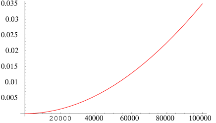
FIG. 3.: LEFT: $\phi~{}{\rm vs.}~{}t$ for a massive dilaton without monopoles: solid=numerics, dashed=our estimate. RIGHT: Relative error in our estimate.

The addition of mass, still keeping the low density condition, produces a small deviation from a constant dilaton, and therefore does not interfere with the standard evolution.

Now we would like to consider the two potential terms together. Since the deviation of the dilaton from a constant in both cases is small, we have no reason to believe that the dilaton will act radically different now. The numerical solution shows that this is indeed a good assumption. The first graph in Figure 4 shows the relative error in estimating the massive low density dilaton in the presence of monopoles as a constant, the second graph shows $\rho_{m}/\rho_{r}$ with the presence of a low density massive dilaton, compared with the standard evolution.

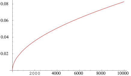
FIG. 4.: LEFT: low density massive dilaton: $\frac{\phi-\phi_{0}}{\phi}$ in the presence of monopoles. RIGHT: $\ln(\rho_{m}/\rho_{r})~{}{\rm vs.}~{}\ln t$: solid=with low density massive $\phi$, dashed=without.

III High Moduli Density

High moduli density era is defined to commence when moduli density becomes comparable to the radiation density. In this era, there is no essential difference between the dilaton (assuming it is heavy enough) and any of the moduli, since the important element is the oscillations around the minimum of the potential rather than the coupling to matter. We have checked this assumption numerically in many cases. Moduli behave here as NR matter, and the universe is MD.

The time dependence of the expansion of the universe with and without the moduli is different, therefore we use for comparison between the two not time but temperature. Using the facts that during RD $H=1.66\sqrt{g_{*}}\frac{T^{2}}{m_{p}}$ (where $g_{*}$ is the effective number of degrees of freedom), and that in our model the evolution begins and ends with RD, we can use H instead of T. We are interested in how the limit on initial ratio of monopole to radiation densities differs when moduli get added to the cosmic mix.

A A Simple Model

The basic idea here is that since during oscillations moduli behave as NR matter, the ratio of moduli to radiation energy will grow roughly as the scale factor a(t), assuming that $g_{*}$ is constant or slowly varying during this period. The universe will very quickly reach moduli domination era in which $\rho_{tot}\simeq\rho_{\phi}\propto a^{-3}$, and $\rho_{m}/\rho_{tot}\propto Const$.

FIG. 5.: $\ln(\rho_{m}/\rho_{tot})~{}{\rm vs.}~{}\ln H$ for various initial conditions. Solid=numerics, dashed$=-1/2$ sloped line. UP LEFT: $\rho_{m}:\rho_{r}:\rho_{\phi}=1:9999:3$. UP RIGHT: $\rho_{m}:\rho_{r}:\rho_{\phi}=1:9999:75$. DOWN LEFT: $\rho_{m}:\rho_{r}:\rho_{\phi}=1:9999:300$. DOWN RIGHT: $\rho_{m}:\rho_{r}:\rho_{\phi}=1:9999:1200$.

Eventually, moduli get converted back into radiation and standard cosmology emerges, with a diluted $\rho_{m}/\rho_{r}$. In the simplest model we parametrize the duration of moduli domination, and imagine the conversion into radiation as an instantaneous and completely efficient process. The graphs in figure 5 show a numerical solution of $\ln(\rho_{m}/\rho_{tot})~{}{\rm vs.}~{}\ln H$. As we can see, a reasonable estimate for $\ln(\rho_{m}/\rho_{tot})$ is provided by a $-1/2$ slope for RD, and a horizontal line for MD. At an arbitrary point $H_{f}$, the moduli decay instantaneously into radiation and therefore once again

$$\ln(\frac{\rho_{m}}{\rho_{tot}})\sim\ln(\frac{\rho_{m}}{\rho_{r}})\sim\ln(a(t))\sim\frac{1}{2}\ln t\sim-\frac{1}{2}\ln H.$$ (26)

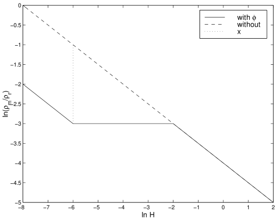
FIG. 6.: $\ln(\rho_{m}/\rho_{tot})~{}{\rm vs.}~{}\ln H$ with and without the moduli.

The difference in the allowed initial monopole to total energy densities can be determined by the vertical distance between the $-1/2$ sloped line and the horizontal line at $H_{f}$ (see Fig. 6). A simple geometrical calculation shows that the relation between the duration of the moduli domination and the effective amount of volume expansion efolds it can replace is given by

$$\left(\rho_{m}/\rho_{tot}\right)_{\rm with}\equiv e^{-x}\left(\rho_{m}/\rho_{tot}\right)_{\rm without},$$ (27)

where

$$x=\frac{1}{2}\ln\left(\frac{H_{i}}{H_{f}}\right).$$ (28)

B A More Realistic Model

Now we would like to treat decay of moduli to radiation in a better way, by including a decay rate in the equations which will govern the duration of moduli domination period. Dimensional arguments lead to the estimate

$$\Gamma\equiv\tau^{-1}\sim m^{3}_{\phi}/m^{2}_{pl}.$$ (29)

The inclusion of such a term is standard [3], and leads to the approximate equation $\dot{\rho}_{\phi}+3H\rho_{\phi}=0$, from which it is clearly seen that moduli really behave as NR matter. This approximate equation holds as long as we can replace $\phi^{2}$ with $\langle\phi^{2}\rangle$, which is justified when oscillations of moduli are much faster than the expansion rate.
If we want to describe the moduli decaying into photons, or other forms of massless particles, we need to correct the conservation equations, moduli density decreases and the radiation density increases,

$$\dot{\rho}_{\phi}+3H\rho_{\phi}=-\Gamma\rho_{\phi}$$ (30)

$$\dot{\rho}_{r}+4(H+\frac{1}{2}\dot{\phi})\rho_{r}=\Gamma\rho_{\phi},$$ (31)

while monopole number conservation still holds. Because the moduli’s oscillations are very fast and we are using averaged values:

$$\langle\phi\rangle=\langle\dot{\phi}\rangle=0.$$ (32)

The approximate equations are given by

$$\dot{\rho}_{\phi}+3H\rho_{\phi}=-\Gamma\rho_{\phi}$$ (33)

$$\dot{\rho}_{r}+4H\rho_{r}=\Gamma\rho_{\phi}$$ (34)

$$3H^{2}=(\frac{1}{4}\dot{\phi}^{2}+\frac{1}{4}m^{2}\phi^{2})+\frac{1}{2}\rho_{r}\approx\frac{1}{2}\rho_{\phi}+\frac{1}{2}\rho_{r},$$ (35)

where in the last equation we have assumed low monopole density. Solving for $\rho_{\phi}$ we obtain

$$\rho_{\phi}=(\rho_{\phi})_{0}e^{-\Gamma(t-t_{0})}(\frac{R}{R_{0}})^{-3},$$ (36)

where $t_{0}$ is the time when oscillations start. Solving for $\rho_{r}$ we obtain

$$\rho_{r}=\left[(\rho_{r})_{0}-\frac{12}{5}\Gamma H_{0}\right]\ \left(\frac{R_{0}}{R}\right)^{4}+\frac{12}{5}\Gamma H_{0}(\frac{R_{0}}{R})^{3/2}.$$ (37)

Therefore soon after moduli begin dominating, radiation density decreases only as $R^{-3/2}$.

As explained, $t_{0}$ is the time which oscillations begin, which is approximately when the moduli come into domination, therefore, $H_{0}=\sqrt{\rho_{\phi}}/m_{p}\approx m_{\phi}^{2}/m_{p}$. At about $t_{rh}=\tau_{\phi}=\Gamma^{-1}$, most of the moduli have decayed into radiation, and the universe re-enters its adiabatic evolution. So between $H_{0}=m_{\phi}^{2}/m_{p}$ and $H_{rh}=1/2t_{rh}=\Gamma/2$, the ratio of monopole to radiation density decreases as $R^{-3/2}\propto H$. Figure 7 shows our approximation for the behavior of $\rho_{m}/\rho_{r}$ with and without moduli. As before, $x$ is the effective amount of volume efolds moduli replaces

$$(\rho_{m}/\rho_{r})_{with}=e^{-x}(\rho_{m}/\rho_{r})_{without}$$ (38)

$$x=\frac{3}{2}\ln(\frac{H_{0}}{H_{rh}})=\frac{3}{2}\ln(\frac{2m_{\phi}^{2}}{\Gamma m_{p}}).$$ (39)

Using the estimate for $\Gamma$ (29) gives

$$x=\frac{3}{2}\ln(\frac{2m_{p}}{m_{\phi}}).$$ (40)

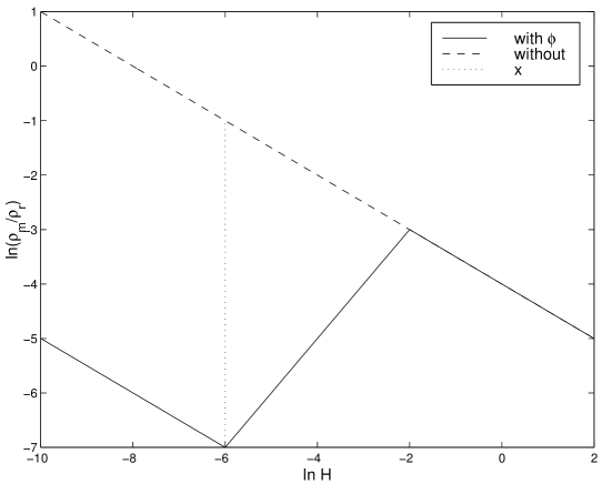
FIG. 7.: $\ln(\rho_{m}/\rho_{r})~{}vs.~{}\ln(H)$: solid=with $\phi$: our approximation, dashed=without $\phi$

Figure 8 shows some comparisons between our approximation and an exact numerical solution for $\rho_{m}/\rho_{r}$. The scale on the the vertical axis $\ln(\rho_{m}/\rho_{r})$ is determined by the choice of initial conditions, and $H$ is in our standard units in which $m_{p}=\sqrt{16\pi}$.

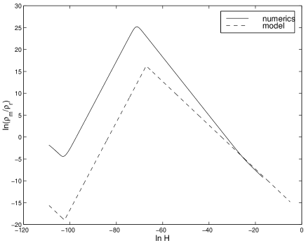
FIG. 8.: $\ln(\rho_{m}/\rho_{r})~{}vs.~{}\ln(H)$, solid=numerics, dashed=our model. UP LEFT: $m=10^{-5}m_{p},~{}\Gamma=10^{-15}m_{p}$, UP RIGHT: $m=10^{-8}m_{p},~{}\Gamma=10^{-24}m_{p}$, DOWN LEFT: $m=10^{-12}m_{p},~{}\Gamma=10^{-36}m_{p}$, DOWN RIGHT: $m=10^{-15}m_{p},~{}\Gamma=10^{-45}m_{p}$.

C Moduli relax the monopole bound

Using (40), we want to derive some consequences regarding how moduli relax the monopole problem.

• As was mentioned in the introduction, in order to solve the monopole problem, we need 27 efolds in volume expansion. If one of the moduli is to supply all 27 on its own, its mass has to be below the upper bound

  $$\frac{3}{2}\ln(\frac{2m_{p}}{m_{\phi}})\stackrel{{\scriptstyle>}}{{{}_{\sim}}}27$$ (41)

  $$m_{\phi}\stackrel{{\scriptstyle<}}{{{}_{\sim}}}10^{-8}m_{p}\approx 10^{8}~{}TeV.$$ (42)

• Since we do not want the monopoles to interfere with nucleosynthesis, we should demand $T_{rh}>10~{}MeV$. We also need to keep in mind that baryogenesis has to occur later. The relationship between the moduli mass and the reheat temperature is:

  $$H_{rh}=1.66\sqrt{g_{*}}\frac{T^{2}_{rh}}{m_{p}}\sim\frac{\Gamma}{2}=\frac{m_{\phi}^{3}}{2m_{p}},$$ (43)

  which requires

  $$m_{\phi}>10^{-14}m_{p}(\frac{g_{*}}{100})^{1/6}\approx 100~{}TeV.$$ (44)

• Moduli should dilute the monopole to radiation ratio before the universe reaches monopole domination. This means that we need $\rho_{m}/\rho_{r}$ at its highest point, $H_{i}$, to be less than unity

  $$(\rho_{m}/\rho_{r})_{i}=(\rho_{m}/\rho_{r})_{c}\sqrt{\frac{H_{c}}{H_{i}}}<1,$$ (45)

  where $H_{c}\approx 10^{10}\sqrt{g_{*}/100}(T_{c}/10^{14}GeV)^{2}GeV$ and $(\rho_{m}/\rho_{r})_{c}\approx 10^{-11}(M_{m}/10^{16}GeV)(10^{14}GeV/T_{c})$, leading to a lower bound on moduli mass,

  $$m_{\phi}>3200\left(\frac{g_{*}}{100}\right)^{1/4}\left((\frac{M_{m}}{10^{14}GeV}\right)GeV.$$ (46)

To summarize our results, here is a table with various values for moduli masses, the amount of (volume) efolds it replaces, its reheat temperature, and whether it acts before monopole domination,

$\bf{m_{\phi}}$	x	$\bf{T_{rh}}$	before md
$10^{-4}~{}eV$	$112$	$2\cdot 10^{-30}~{}MeV$	no
$10^{5}~{}GeV$	$49$	$2~{}MeV$	yes
$10^{8}~{}GeV$	$39$	$6\cdot 10^{4}~{}MeV$	yes
$10^{11}~{}GeV$	$29$	$2\cdot 10^{9}~{}MeV$	yes
$10^{12}~{}GeV$	$25$	$6\cdot 10^{10}~{}MeV$	yes
$10^{14}~{}GeV$	$18$	$6\cdot 10^{13}~{}MeV$	yes

TABLE I.: $x$ values for different moduli mass.

IV Discussion

• The mechanism described here makes use of massive scalar fields that decay into radiation. String theory provides us with several candidate fields – moduli (including the dilaton). Instead of demanding that a single field provides all the 27 efolds, a possible scenario is that two or maybe more fields have different masses and therefore oscillate at different times, and each of them contributes a few of the needed efolds. As an example, consider two fields, one with mass of $10^{8}~{}GeV$, and the other with mass of $10^{12}~{}GeV$. We will assume that for both fields the decay rate is given by (29). The $10^{12}~{}GeV$ mass field begins to dominate when $\ln(H_{i})=\ln(\frac{m^{2}}{m_{p}})\sim 11.5$, and ends at $\ln(H_{rh})=\ln(\frac{m^{3}}{m^{2}_{p}})\sim-5.2$. During this time it provides 25 efolds. Only later does the $10^{8}~{}GeV$ mass field reaches domination, at $\ln(H_{i})=-6.9$ until $\ln(H_{rh})\sim-32.9$, and it provides additional 39 efolds. Therefore, it is possible to use use several heavier fields instead of a single lighter one.

• The presence of moduli changes the standard adiabatic evolution of the universe, introducing a period (or periods) of matter domination. Looking at how many decades of temperature were indeed matter dominated will quantify the deviation from the standard evolution,

  $$\ln(\frac{T_{i}}{T_{rh}})=\ln(\sqrt{\frac{H_{i}}{H_{rh}}})\sim\frac{1}{2}\ln(\frac{\Gamma m_{p}}{2m^{2}}),$$ (47)

  and using (29),

  $$\ln(\frac{T_{i}}{T_{rh}})\sim\frac{1}{2}\ln(\frac{m}{2m_{p}}).$$ (48)

  Looking at (40) shows that the relation between $x$ and the deviation is linear. We conclude that to substantially relax the monopole bound long periods of coherent oscillation are required.

We want to to compare our estimate to the numerical results. Table II shows the numerical and the estimated $x$ values, and the relative error ($E_{x}=\frac{x_{num}-x_{est}}{x_{num}}$):

$\bf{m}$	$\bf{\Gamma}$	$\bf{x_{est}}$	$\bf{x_{num}}$	$\bf{E_{x}}$
$10^{-5}m_{p}$	$10^{-15}m_{p}$	$18.3$	$9.8$	$-87\%$
$10^{-8}m_{p}$	$10^{-24}m_{p}$	$28.7$	$18.6$	$-54\%$
$10^{-12}m_{p}$	$10^{-36}m_{p}$	$42.5$	$30.3$	$-40\%$
$10^{-15}m_{p}$	$10^{-45}m_{p}$	$52.8$	$39.2$	$-35\%$
$10^{-18}m_{p}$	$10^{-54}m_{p}$	$63.2$	$47.5$	$-33\%$

TABLE II.: Accuracy of analytical estimates of $x$.

As can be seen, our estimated values improve as the decay rate (and moduli’s mass) get smaller. Also, there is a systematic “overshooting” (estimating too big an $x$). We understand this effect the following way, our calculation assumes that immediately as the moduli come to domination they begin to oscillate and the $\Gamma$ term becomes effective. Looking at Figure 8, we see that there is a period in which moduli dominate and therefore the universe is MD ($R\propto t^{2/3}$), yet the $\Gamma$ term is not operative. This results in $\frac{\rho_{m}}{\rho_{r}}\propto H^{-2/3}$ instead of $H^{-1/2}$, thus the numerical results give values that are lower than our estimate.

We can try to improve our simple estimate by taking into account this rise, define $H_{m}$ such that between $H_{i}$ and $H_{m}$ the universe is MD, but the moduli do not yet oscillate. Only below $H_{m}$ the oscillations and the moduli decay start. Following [3], $H_{m}=\sqrt{\frac{m^{2}\Gamma}{m_{p}}}$. Such a calculation will yield $x=\frac{2}{3}\ln(\frac{2^{9/4}m^{2}}{\Gamma m_{p}})=\frac{2}{3}\ln(\frac{2^{9/4}m_{p}}{m})$, which compared with the numerical values of $x$ is consistently “undershooting” (estimating too small an $x$). We have obtained an upper bound on $x$ as well as a lower bound, and for the best estimated value we can take their average, $x_{av}=\ln(\frac{2^{3/2}m_{p}^{13/12}}{m^{13/12}})$. Table III summarizes the relative error in the upper and lower bounds, as well as in the average,

$\bf{m}$	$\bf{\Gamma}$	$\bf{x_{av}}$	$\bf{E_{x}(upper~{}bound)}$	$\bf{E_{x}(lower~{}bound)}$	$\bf{E_{x}(average)}$
$10^{-5}m_{p}$	$10^{-15}m_{p}$	$13.5$	$-87\%$	$+11\%$	$-38\%$
$10^{-8}m_{p}$	$10^{-24}m_{p}$	$21.0$	$-54\%$	$+28\%$	$-13\%$
$10^{-12}m_{p}$	$10^{-36}m_{p}$	$31.0$	$-40\%$	$+36\%$	$-2\%$
$10^{-15}m_{p}$	$10^{-45}m_{p}$	$38.5$	$-35\%$	$+39\%$	$+2\%$
$10^{-18}m_{p}$	$10^{-54}m_{p}$	$46.0$	$-33\%$	$+40\%$	$+3\%$

TABLE III.: Errors in analytical estimates of $x$.

To illustrate the two bounds, Figure 9 shows the two bounds and the numerical behavior, for $m=10^{-15}m_{p}$.

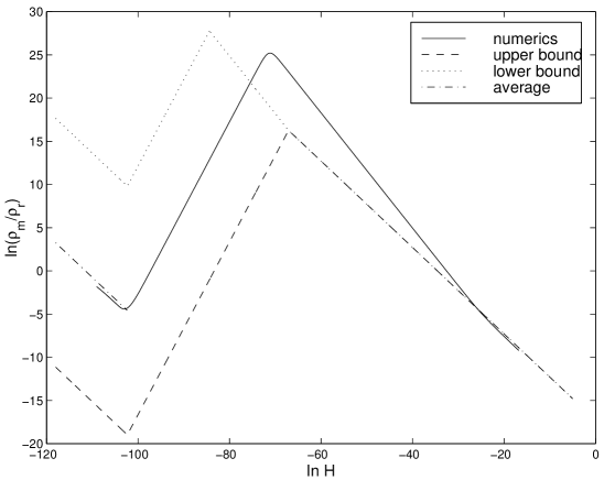
FIG. 9.: Approximate evolution, $\Gamma=10^{-15}m_{p}$ solid=numerics, dotted=upper bound, dashed=lower bound, dashed-dotted=the average.

REFERENCES

• [1] J. Polchinski, String Theory, Cambridge University Press, 1998.
• [2] A. D. Linde, Particle Physics and Inflationary Cosmology, Harwood Academic, 1990.
• [3] E. W. Kolb and M. S. Turner, The Early Universe, Addison-Wesley, 1993.
• [4] G. Dvali and L.M. Krauss, hep-ph/9811298.
• [5] G. Dvali, H. Liu and T. Vachaspati, Phys. Rev. Lett. 80, 2281 (1998).
• [6] G. Dvali, A. Melfo and G. Senjanovic, Phys. Rev. Lett. 75, 4559 (1995).
• [7] B. Bajc, A. Riotto and G. Senjanovic, Mod. Phys. Lett. A13, 2955 (1998).
• [8] J. Preskill, Phys. Rev. Lett. 43, 1365 (1979).
• [9] P. Langacker and S.-Y. Pi, Phys. Rev. Lett. 45, 1 (1980).
• [10] A. H. Guth, Phys. Rev. D 23, 347 (1981).
• [11] A.A. Tseytlin and C. Vafa, Nucl. Phys. B372, 443 (1992).
• [12] T. Barreiro, B.B. de Carlos and E.J. Copeland, Phys. Rev. D58, 083513 (1998).
• [13] T. Banks, M. Berkooz and P.J. Steinhardt, Phys. Rev. D52, 705 (1995).
• [14] K. Choi, E.J. Chun and H.B. Kim, Phys. Rev. D58, 046003 (1998).
• [15] K. Choi, H.B. Kim and H. Kim, hep-th/9808122.
• [16] G. Lazarides, R. Schaefer, D. Seckel and Q. Shafi, Nucl. Phys. B346, 193 (1990).
• [17] T. Banks and M. Dine, Nucl. Phys. B505, 445 (1996).