INTRODUCTION TO ELECTROWEAK SYMMETRY BREAKING

An introduction to the physics of electroweak symmetry breaking is given. We discuss Higgs boson production in $e^{+}e^{-}$ and hadronic collisions and survey search techniques at present and future accelerators. Indirect limits on the Higgs boson mass from triviality arguments, vacuum stability, and precision electroweak measurements are presented. An effective Lagrangian, valid when there is no low mass Higgs boson, is used to discuss the physics of a strongly interacting electroweak symmetry breaking sector. Finally, the Higgs bosons of the minimal supersymmetric model are considered, along with the resulting differences in phenomenology from the Standard Model.

1 Introduction

The search for the Higgs boson has become a major focus of all particle accelerators. In the simplest version of the electroweak theory, the Higgs boson serves both to give the $W$ and $Z$ bosons their masses and to give the fermions mass. It is thus a vital part of the theory. In these lectures, we will introduce the Higgs boson of the Standard Model of electroweak interactions.$\!{}^{{\bf?},{\bf?}}$

Section 2 contains a derivation of the Higgs mechanism, with particular attention to the choice of gauge. In Section 3 we discuss indirect limits on the Higgs boson mass coming from theoretical arguments and from precision measurements at the LEP and LEP2 colliders. The production of the Standard Model Higgs boson is then summarized in Sections 4 - 8, beginning with a discussion of the Higgs boson branching ratios in Section 4. Higgs production in $e^{+}e^{-}$ collisions at LEP and LEP2 and in hadronic collisions at the Tevatron and the LHC are discussed in Sections 5 and 6, with an emphasis on the potential for discovery in the different channels.

Section 7 contains a derivation of the effective $W$ approximation and a discussion of Higgs production through vector boson fusion at the LHC. The potential for a Higgs boson discovery at a very high energy $e^{+}e^{-}$ collider, ($\sqrt{s}>500~{}GeV$) is discussed in Section 8.

Suppose the Higgs boson is not discovered in an $e^{+}e^{-}$ collider or at the LHC? Does this mean the Standard Model with a Higgs boson must be abandoned? In Section 9, we discuss the implications of a very heavy Higgs boson, ($M_{h}>>800~{}GeV$). In this regime the $W$ and $Z$ gauge bosons are strongly interacting and new techniques must be used. We present an effective Lagrangian valid for the case where $M_{h}>>\sqrt{s}$.

Section 10 contains a list of some of the objections which many theorists have to the minimal Standard Model with a single Higgs boson. One of the most popular alternatives to the minimal Standard Model is to make the theory supersymmetric. The Higgs sector of the minimal supersymmetric model (MSSM) is surveyed in Section 11. We end with some conclusions in Section 12.

2 The Higgs Mechanism

2.1 Abelian Higgs Model

The central question of electroweak physics is :“Why are the $W$ and $Z$ boson masses non-zero?” The measured values, $M_{W}=80~{}GeV$ and $M_{Z}=91~{}GeV$, are far from zero and cannot be considered as small effects. To see that this is a problem, we consider a $U(1)$ gauge theory with a single gauge field, the photon. The Lagrangian is simply$\!{}^{{\bf?}}$

$${\cal L}=-{1\over 4}F_{\mu\nu}F^{\mu\nu},$$ (1)

where

$$F_{\mu\nu}=\partial_{\nu}A_{\mu}-\partial_{\mu}A_{\nu}.$$ (2)

The statement of local $U(1)$ gauge invariance is that the Lagrangian is invariant under the transformation:$A_{\mu}(x)\rightarrow A_{\mu}(x)-\partial_{\mu}\eta(x)$ for any $\eta$ and $x$. Suppose we now add a mass term for the photon to the Lagrangian,

$${\cal L}=-{1\over 4}F_{\mu\nu}F^{\mu\nu}+{1\over 2}m^{2}A_{\mu}A^{\mu}.$$ (3)

It is easy to see that the mass term violates the local gauge invariance. It is thus the $U(1)$ gauge invariance which requires the photon to be massless.

We can extend the model by adding a single complex scalar field with charge $-e$ which couples to the photon. The Lagrangian is now,

$${\cal L}=-{1\over 4}F_{\mu\nu}F^{\mu\nu}+\mid D_{\mu}\phi\mid^{2}-V(\phi),$$ (4)

where

$$D_{\mu} = \partial_{\mu}-ieA_{\mu}$$

$$V(\phi) = \mu^{2}\mid\phi\mid^{2}+\lambda(\mid\phi\mid^{2})^{2}.$$ (5)

$V(\phi)$ is the most general renormalizable potential allowed by the $U(1)$ gauge invariance.

This Lagrangian is invariant under global $U(1)$ rotations, $\phi\rightarrow e^{i\theta}\phi$, and also under local gauge transformations:

$$A_{\mu}(x) \rightarrow A_{\mu}(x)-\partial_{\mu}\eta(x)$$

$$\phi(x) \rightarrow e^{-ie\eta(x)}\phi(x).$$ (6)

Figure 1: Scalar potential with $\mu^{2}>0$.

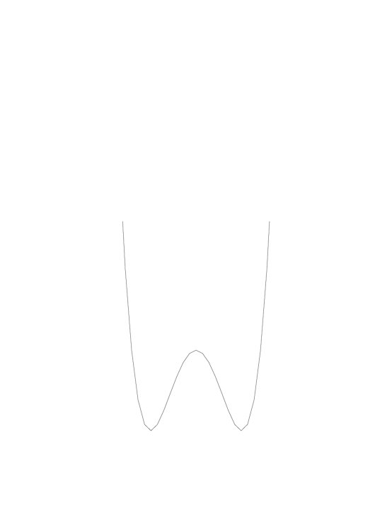
Figure 2: Scalar potential with $\mu^{2}<0$.

There are now two possibilities for the theory. If $\mu^{2}>0$ the potential has the shape shown in Fig. 1 and preserves the symmetries of the Lagrangian. The state of lowest energy is that with $\phi=0$, the vacuum state. The theory is simply quantum electrodynamics with a massless photon and a charged scalar field $\phi$ with mass $\mu$.

The alternative scenario is more interesting. In this case $\mu^{2}<0$ and the potential can be written as, $\!{}^{{\bf?},{\bf?}}$

$$V(\phi)=-\mid\mu^{2}\mid\mid\phi\mid^{2}+\lambda(\mid\phi\mid^{2})^{2},$$ (8)

which has the Mexican hat shape shown in Fig. 2. In this case the minimum energy state is not at $\phi=0$ but rather at

$$\langle\phi\rangle=\sqrt{-{\mu^{2}\over 2\lambda}}\equiv{v\over\sqrt{2}}.$$ (9)

$\langle\phi\rangle$ is called the vacuum expectation value (VEV) of $\phi$. Note that the direction in which the vacuum is chosen is arbitrary, but it is conventional to choose it to lie along the direction of the real part of $\phi$. The VEV then clearly breaks the global $U(1)$ symmetry.

It is convenient to rewrite $\phi$ as

$$\phi\equiv{1\over\sqrt{2}}e^{i{\chi\over v}}\biggl{(}v+h\biggr{)},$$ (10)

where $\chi$ and $h$ are real fields which have no VEVs. If we substitute Eq. 10 back into the original Lagrangian, the interactions in terms of the fields with no VEVs can be found,

$${\cal L} = -{1\over 4}F_{\mu\nu}F^{\mu\nu}-evA_{\mu}\partial^{\mu}\chi+{e^{2}v^{2}\over 2}A_{\mu}A^{\mu}$$ (11)

$$+{1\over 2}\biggl{(}\partial_{\mu}h\partial^{\mu}h+2\mu^{2}h^{2}\biggr{)}+{1\over 2}\partial_{\mu}\chi\partial^{\mu}\chi$$

$$+(h,~{}\chi{\rm~{}interactions}).$$

Eq. 11 describes a theory with a photon of mass $M_{A}=ev$, a scalar field $h$ with mass-squared $-2\mu^{2}>0$, and a massless scalar field $\chi$. The mixed $\chi-A$ propagator is confusing, however. This term can be removed by making a gauge transformation:

$$A^{\prime}_{\mu}\equiv A_{\mu}-{1\over ev}\partial_{\mu}\chi.$$ (12)

After making the gauge transformation of Eq. 12 the $\chi$ field disappears from the theory and we say that it has been “eaten” to give the photon mass. This is called the Higgs mechanism and the $\chi$ field is often called a Goldstone boson.$\!{}^{{\bf?}}$ In the gauge of Eq. 12 the particle content of the theory is apparent; a massive photon and a scalar field $h$, which we call a Higgs boson. The Higgs mechanism can be summarized by saying that the spontaneous breaking of a gauge theory by a non-zero VEV results in the disappearance of a Goldstone boson and its transformation into the longitudinal component of a massive gauge boson.

It is instructive to count the number of degrees of freedom (dof). Before the spontaneous symmetry breaking there was a massless photon (2 dof) and a complex scalar field (2 dof) for a total of 4 degrees of freedom. After the spontaneous symmetry breaking there is a massive photon (3 dof) and a real scalar, $h$, (1 dof) for the same total number of degrees of freedom.

At this point let us consider the gauge dependance of these results. The gauge choice above with the transformation $A_{\mu}^{\prime}=A_{\mu}-{1\over ev}\partial_{\mu}\chi$ is called the unitary gauge. This gauge has the advantage that the particle spectrum is obvious and there is no $\chi$ field. The unitary gauge, however, has the disadvantage that the photon propagator, $\Delta_{\mu\nu}(k)$, has bad high energy behaviour,

$$\Delta_{\mu\nu}(k)=-{i\over k^{2}-M_{A}^{2}}\biggl{(}g_{\mu\nu}-{k^{\mu}k^{\nu}\over M_{A}^{2}}\biggr{)}.$$ (13)

In the unitary gauge, scattering cross sections have contributions which grow with powers of $k^{2}$ (such as $k^{4}$, $k^{6}$, etc.) which cannot be removed by the conventional mass, coupling constant, and wavefunction renormalizations. More convenient gauges are the $R_{\xi}$ gauges which are obtained by adding the gauge fixing term to the Lagrangian,$\!{}^{{\bf?}}$

$${\cal L}_{GF}=-{1\over 2\xi}\biggl{(}\partial_{\mu}A^{\mu}+\xi ev\chi\biggl{)}^{2}.$$ (14)

Different choices for $\xi$ correspond to different gauges. In the limit $\xi\rightarrow\infty$ the unitary gauge is recovered. Note that after integration by parts the cross term in Eq.  14 exactly cancels the mixed $\chi\partial_{\mu}A^{\mu}$ term of Eq. 11. The gauge boson propagator in $R_{\xi}$ gauge is given by

$$\Delta_{\mu\nu}(k)=-{i\over k^{2}-M_{A}^{2}}\biggl{(}g_{\mu\nu}-{(1-\xi)k_{\mu}k_{\nu}\over k^{2}-\xi M_{A}^{2}}\biggr{)}.$$ (15)

In the $R_{\xi}$ gauges the $\chi$ field is part of the spectrum and has mass $M_{\chi}^{2}=\xi M_{A}^{2}$. Feynman gauge corresponds to the choice $\xi=1$ and has a massive Goldstone boson, $\chi$, while Landau gauge has $\xi=0$ and the Goldstone boson $\chi$ is massless with no coupling to the physical Higgs boson. The Landau gauge is often the most convenient for calculations involving the Higgs boson since there is no coupling to the unphysical $\chi$ field.

2.2 Weinberg-Salam Model

It is now straightforward to obtain the usual Weinberg-Salam model of electroweak interactions.$\!{}^{{\bf?}}$ The Weinberg- Salam model is an $SU(2)_{L}\times U(1)_{Y}$ gauge theory containing three $SU(2)_{L}$ gauge bosons, $W_{\mu}^{i}$, $i=1,2,3$, and one $U(1)_{Y}$ gauge boson, $B_{\mu}$, with kinetic energy terms,

$${\cal L}_{\rm KE}=-{1\over 4}W_{\mu\nu}^{i}W^{\mu\nu i}-{1\over 4}B_{\mu\nu}B^{\mu\nu}\quad,$$ (16)

where

$$W_{\mu\nu}^{i} = \partial_{\nu}W_{\mu}^{i}-\partial_{\mu}W_{\nu}^{i}+g\epsilon^{ijk}W_{\mu}^{j}W_{\nu}^{k}\quad,$$

$$B_{\mu\nu} = \partial_{\nu}B_{\mu}-\partial_{\mu}B_{\nu}\quad.$$ (17)

Coupled to the gauge fields is a complex scalar $SU(2)$ doublet, $\Phi$,

$$\Phi=\left(\begin{array}[]{c}\phi^{+}\\ \phi^{0}\end{array}\right)$$ (18)

with a scalar potential given by

$$V(\Phi)=\mu^{2}\mid\Phi^{\dagger}\Phi\mid+\lambda\biggl{(}\mid\Phi^{\dagger}\Phi\mid\biggr{)}^{2}\quad,$$ (19)

($\lambda>0$). This is the most general renormalizable and $SU(2)_{L}$ invariant potential allowed.

Just as in the Abelian model of Section 2.1, the state of minimum energy for $\mu^{2}<0$ is not at $\Phi=0$ and the scalar field develops a VEV. The direction of the minimum in $SU(2)_{L}$ space is not determined since the potential depends only on the combination $\Phi^{\dagger}\Phi$ and we arbitrarily choose

$$\langle\Phi\rangle={1\over\sqrt{2}}\left(\begin{array}[]{c}0\\ v\end{array}\right)\quad.$$ (20)

With this choice the scalar doublet has $U(1)_{Y}$ charge (hypercharge) $Y_{\Phi}=1$ and the electromagnetic charge is

$$Q={(\tau_{3}+Y)\over 2}\,\,.$$ (21)

Therefore,

$$Q\langle\Phi\rangle=0$$ (22)

and electromagnetism is unbroken by the scalar VEV. The VEV of Eq. 20 hence yields the desired symmetry breaking scheme,

$$SU(2)_{L}\times U(1)_{Y}\rightarrow U(1)_{EM}.$$ (23)

It is now straightforward to see how the Higgs mechanism generates masses for the $W$ and $Z$ gauge bosons in the same fashion as a mass was generated for the photon in the Abelian Higgs model of Section 2.1. The contribution of the scalar doublet to the Lagrangian is,

$${\cal L}_{s}=(D^{\mu}\Phi)^{\dagger}(D_{\mu}\Phi)-V(\Phi)\quad,$$ (24)

where

$$D_{\mu}=\partial_{\mu}+i{g\over 2}\tau\cdot W_{\mu}+i{g^{\prime}\over 2}B_{\mu}Y.$$ (25)

In unitary gauge there are no Goldstone bosons and only the physical Higgs scalar remains in the spectrum after the spontaneous symmetry breaking has occurred. Therefore the scalar doublet in unitary gauge can be written as

$$\Phi={1\over\sqrt{2}}\left(\begin{array}[]{c}0\\ v+h\end{array}\right)\quad,$$ (26)

which gives the contribution to the gauge boson masses from the scalar kinetic energy term of Eq. 24,

$${1\over 2}(0,v)\biggl{(}{1\over 2}g\tau\cdot W_{\mu}+{1\over 2}g^{\prime}B_{\mu}\biggr{)}^{2}\left(\begin{array}[]{c}0\\ v\end{array}\right).$$ (27)

The physical gauge fields are then two charged fields, $W^{\pm}$, and two neutral gauge bosons, $Z$ and $\gamma$.

$$W^{\pm}_{\mu} = {1\over\sqrt{2}}(W_{\mu}^{1}\mp iW_{\mu}^{2})$$

$$Z^{\mu} = {-g^{\prime}B_{\mu}+gW_{\mu}^{3}\over\sqrt{g^{2}+g^{\prime~{}2}}}$$

$$A^{\mu} = {gB_{\mu}+g^{\prime}W_{\mu}^{3}\over\sqrt{g^{2}+g^{\prime~{}2}}}.$$ (28)

The gauge bosons obtain masses from the Higgs mechanism:

$$M_{W}^{2} = {1\over 4}g^{2}v^{2}$$

$$M_{Z}^{2} = {1\over 4}(g^{2}+g^{\prime~{}2})v^{2}$$

$$M_{A} = 0.$$ (29)

Since the massless photon must couple with electromagnetic strength, $e$, the coupling constants define the weak mixing angle $\theta_{W}$,

$$e = g\sin\theta_{W}$$

$$e = g^{\prime}\cos\theta_{W}\quad.$$ (30)

It is instructive to count the degrees of freedom after the spontaneous symmetry breaking has occurred. We began with a complex scalar $SU(2)_{L}$ doublet $\Phi$ with four degrees of freedom, a massless $SU(2)_{L}$ gauge field, $W_{i}$, with six degrees of freedom and a massless $U(1)_{Y}$ gauge field, $B$, with 2 degrees of freedom for a total of $12$. After the spontaneous symmetry breaking there remains a physical real scalar field $h$ ($1$ degree of freedom), massive $W$ and $Z$ fields ($9$ degrees of freedom), and a massless photon ($2$ degrees of freedom). We say that the scalar degrees of freedom have been “eaten” to give the $W^{\pm}$ and $Z$ gauge bosons their longitudinal components.

Just as in the case of the Abelian Higgs model, if we go to a gauge other than unitary gauge, there will be Goldstone bosons in the spectrum and the scalar field can be written,

$$\Phi={1\over\sqrt{2}}e^{i{\omega\cdot\tau\over 2v}}\left(\begin{array}[]{c}0\\ v+h\end{array}\right).$$ (31)

In the Standard Model, there are three Goldstone bosons, ${\vec{\omega}}=(\omega^{\pm},z)$, with masses $M_{W}$ and $M_{Z}$ in the Feynman gauge. These Goldstone bosons will play an important role in our understanding of the physics of a very heavy Higgs boson, as we will discuss in Section 9.

Fermions can easily be included in the theory and we will consider the electron and its neutrino as an example. It is convenient to write the fermions in terms of their left- and right-handed projections,

$$\psi_{L,R}={1\over 2}(1\mp\gamma_{5})\psi\,\,.$$ (32)

From the four-Fermi theory of weak interactions, we know that the $W$-boson couples only to left-handed fermions and so we construct the $SU(2)_{L}$ doublet,

$$L_{L}=\left(\begin{array}[]{c}\nu_{L}\\ e_{L}\end{array}\right).$$ (33)

From Eq. 21, the hypercharge of the lepton doublet must be $Y_{L}=-1$. Since the neutrino is (at least approximately) massless, it can have only one helicity state which is taken to be $\nu_{L}$. Experimentally, we know that right-handed fields do not interact with the $W$ boson, and so the right-handed electron, $e_{R}$, must be an $SU(2)_{L}$ singlet and so has $Y_{e_{R}}=-2$. Using these hypercharge assignments, the leptons can be coupled in a gauge invariant manner to the $SU(2)_{L}\times U(1)_{Y}$ gauge fields,

$${\cal L}_{lepton}=i{\overline{e}}_{R}\gamma^{\mu}\biggl{(}\partial_{\mu}+i{g^{\prime}\over 2}Y_{e}B_{\mu}\biggr{)}e_{R}+i{\overline{L}}_{L}\gamma^{\mu}\biggl{(}\partial_{\mu}+i{g\over 2}\tau\cdot W_{\mu}+i{g^{\prime}\over 2}Y_{L}B_{\mu}\biggr{)}L_{L}\,\,.$$ (34)

All of the known fermions can be accommodated in the Standard Model in an identical manner as was done for the leptons. The $SU(2)_{L}$ and $U(1)_{Y}$ charge assignments of the first generation of fermions are given in Table 1.

Table 1: Fermion Fields of the Standard Model Field SU(3) $SU(2)_{L}$ $U(1)_{Y}$ $Q_{L}=\left(\begin{array}[]{c}u_{L}\\ d_{L}\end{array}\right)$ $3$ $2$ $~{}{1\over 3}$ $u_{R}$ $3$ $1$ ${4\over 3}$ $d_{R}$ $3$ $1$ $~{}-{2\over 3}$ $L_{L}=\left(\begin{array}[]{c}\nu_{L}\\ e_{L}\end{array}\right)$ $1$ $2$ $~{}-1$ $e_{R}$ $1$ $1$ $~{}-2$ $\Phi=\left(\begin{array}[]{c}\phi^{+}\\ \phi^{0}\end{array}\right)$ $1$ $2$ $1$

A fermion mass term takes the form

$${\cal L}_{mass}=-m{\overline{\psi}}\psi=-m\biggl{(}{\overline{\psi}}_{L}\psi_{R}+{\overline{\psi}}_{R}\psi_{L}\biggr{)}\,\,.$$ (35)

As is obvious from Table 1, the left-and right-handed fermions transform differently under $SU(2)_{L}$ and $U(1)_{Y}$ and so gauge invariance forbids a term like Eq. 35. The Higgs boson can be used to give the fermions mass, however. The gauge invariant Yukawa coupling of the Higgs boson to the up and down quarks is

$${\cal L}_{d}=-\lambda_{d}{\overline{Q}}_{L}\Phi d_{R}+h.c.\quad,$$ (36)

This gives the effective coupling

$$-\lambda_{d}{1\over\sqrt{2}}({\overline{u}}_{L},~{}{\overline{d}}_{L})\left(\begin{array}[]{c}0\\ v+h\end{array}\right)d_{R}+h.c.$$ (37)

which can be seen to yield a mass term for the down quark if we make the identification

$$\lambda_{d}={m_{d}\sqrt{2}\over v}.$$ (38)

In order to generate a mass term for the up quark we use the fact that $\Phi^{c}\equiv-i\tau_{2}\Phi^{*}$ is an $SU(2)_{L}$ doublet and we can write the $SU(2)_{L}$ invariant coupling

$${\cal L}_{u}=-\lambda_{u}{\overline{Q}}_{L}\Phi^{c}u_{R}+h.c.$$ (39)

which generates a mass term for the up quark. Similar couplings can be used to generate mass terms for the charged leptons. Since the neutrino has no right handed partner, it remains massless.

For the multi-family case, the Yukawa couplings, $\lambda_{d}$ and $\lambda_{u}$, become $N_{F}\times N_{F}$ matrices (where $N_{F}$ is the number of families). Since the fermion mass matrices and Yukawa matrices are proportional, the interactions of the Higgs boson with the fermion mass eigenstates are flavor diagonal and the Higgs boson does not mediate flavor changing interactions. (In models with extended Higgs sectors, this need not be the case.)

By expressing the fermion kinetic energy in terms of the gauge boson mass eigenstates of Eq. 28, the charged and neutral weak current interactions of the fermions can be found. A complete set of Feynman rules for the interactions of the fermions and gauge bosons of the Standard Model is given in Ref. 3.

The parameter $v$ can be found from the charged current for $\mu$ decay, $\mu\rightarrow e{\overline{\nu}}_{e}\nu_{\mu}$, as shown in Fig. 3. The interaction strength for muon decay is measured very accurately to be $G_{F}=1.16639\times 10^{-5}~{}GeV^{-2}$ and can be used to determine $v$.

Figure 3: Determination of the vacuum expectation value $v$ from $\mu$ decay.

Since the momentum carried by the $W$ boson is of order $m_{\mu}$ it can be neglected in comparison with $M_{W}$ and we make the identification

$${G_{F}\over\sqrt{2}}={g^{2}\over 8M_{W}^{2}}={1\over 2v^{2}},$$ (40)

which gives the result

$$v=(\sqrt{2}G_{F})^{-1/2}=246~{}GeV\,\,.$$ (41)

One of the most important points about the Higgs mechanism is that all of the couplings of the Higgs boson to fermions and gauge bosons are completely determined in terms of coupling constants and fermion masses. The potential of Eq. 19 had two free parameters, $\mu$ and $\lambda$. We can trade these for

$$v^{2} = -{\mu^{2}\over 2\lambda}$$

$$M_{h}^{2} = 2v^{2}\lambda.$$ (42)

There are no remaining adjustable parameters and so Higgs production and decay processes can be computed unambiguously in terms of the Higgs mass alone.

3 Indirect Limits on the Higgs Boson Mass

Before we discuss the experimental searches for the Higgs boson, it is worth considering some theoretical constraints on the Higgs boson mass. Unfortunately, these constraints can often be evaded by postulating the existence of some unknown new physics which enters into the theory at a mass scale above that of current experiments, but below the Planck scale. Never the less, in the minimal Standard Model where there is no new physics between the electroweak scale and the Planck scale, there exist both upper and lower bounds on the Higgs boson mass.

3.1 Triviality

Bounds on the Higgs boson mass have been deduced on the grounds of triviality.$\!{}^{{\bf?},{\bf?}}$ The basic argument goes as follows: Consider a pure scalar theory in which the potential is given by

$$V(\Phi)=\mu^{2}\mid\Phi^{\dagger}\Phi\mid+\lambda(\mid\Phi^{\dagger}\Phi\mid)^{2}$$ (43)

where the quartic coupling is

$$\lambda={M_{h}^{2}\over 2v^{2}}.$$ (44)

This is the scalar sector of the Standard Model with no gauge bosons or fermions. The quartic coupling, $\lambda$, changes with the effective energy scale $Q$ due to the self interactions of the scalar field:

$${d\lambda\over dt}={3\lambda^{2}\over 4\pi^{2}},$$ (45)

where $t\equiv\log(Q^{2}/Q_{0}^{2})$ and $Q_{0}$ is some reference scale. (The reference scale is often taken to be $v$ in the Standard Model.) Eq. 45 is easily solved,

$${1\over\lambda(Q)} = {1\over\lambda(Q_{0})}-{3\over 4\pi^{2}}\log\biggl{(}{Q^{2}\over Q^{2}_{0}}\biggr{)},$$

$$\lambda(Q) = {\lambda(Q_{0})\over\biggl{[}1-{3\lambda(Q_{0})\over 4\pi^{2}}\log({Q^{2}\over Q^{2}_{0}})\biggr{]}}.$$ (46)

Hence if we measure $\lambda$ at some energy scale, we can predict what it will be at all other energy scales. From Eq.  46 we see that $\lambda(Q)$ blows up as $Q\rightarrow\infty$ (called the Landau pole). Regardless of how small $\lambda(Q_{0})$ is, $\lambda(Q)$ will eventually become infinite at some large $Q$. Alternatively, $\lambda(Q_{0})\rightarrow 0$ as $Q\rightarrow 0$ with $\lambda(Q)>0$. Without the $\lambda\Phi^{4}$ interaction of Eq. 43 the theory becomes a non-interacting theory at low energy, termed a trivial theory.

To obtain a bound on the Higgs mass we require that the quartic coupling be finite,

$${1\over\lambda(\Lambda)}>0,$$ (47)

where $\Lambda$ is some large scale where new physics enters in. Taking the reference scale $Q_{0}=v$, and substituting Eq. 44 gives an approximate upper bound on the Higgs mass,

$$M_{h}^{2}<{8\pi^{2}v^{2}\over 3\log(\Lambda^{2}/v^{2})}\quad.$$ (48)

Requiring that there be no new physics before $10^{16}~{}GeV$ yields the approximate upper bound on the Higgs boson mass,

$$M_{h}<160~{}GeV.$$ (49)

As the scale $\Lambda$ becomes smaller, the limit on the Higgs mass becomes progressively weaker and for $\Lambda\sim 3~{}TeV$, the bound is roughly $M_{h}<600~{}GeV$. Of course, this picture is valid only if the one loop evolution equation of Eq. 45 is an accurate description of the theory at large $\lambda$. For large $\lambda$, however, higher order or non-perturbative corrections to the evolution equation must be included.$\!{}^{{\bf?}}$

Lattice gauge theory calculations have used similar techniques to obtain a bound on the Higgs mass. As above, they consider a purely scalar theory and require that the scalar self coupling $\lambda$ remain finite for all scales less than some cutoff which is arbitrarily chosen to be $2\pi M_{h}$. This gives a limit$\!{}^{{\bf?}}$

$$M_{h}({\rm lattice})<640~{}GeV.$$ (50)

The lattice results are relatively insensitive to the value of the cutoff chosen. Note that this bound is in rough agreement with that found above for $\Lambda\sim 3~{}TeV$.

Of course everything we have done so far is for a theory with only scalars. The physics changes dramatically when we couple the theory to fermions and gauge bosons. Since the Higgs coupling to fermions is proportional to the Higgs boson mass, the most relevant fermion is the top quark. Including the top quark and the gauge bosons, Eq.  45 becomes$\!{}^{{\bf?}}$

$${d\lambda\over dt}={1\over 16\pi^{2}}\biggl{[}12\lambda^{2}+12\lambda g_{t}^{2}-12g_{t}^{4}-{3\over 2}\lambda(3g^{2}+g^{\prime~{}2})+{3\over 16}(2g^{4}+(g^{2}+g^{\prime~{}2})^{2})\biggr{]}$$ (51)

where

$$g_{t}\equiv-{M_{t}\over v}\quad.$$ (52)

For a heavy Higgs boson , $\lambda>g_{t},g,g^{\prime}$, and the dominant contributions to the running of $\lambda$ are,

$${d\lambda\over dt}\sim{\lambda\over 16\pi^{2}}\biggl{[}12\lambda+12g_{t}^{2}-{3\over 2}(3g^{2}+g^{\prime~{}2})\biggr{]}.$$ (53)

There is a critical value of the quartic coupling $\lambda$ which depends on the top quark mass,

$$\lambda_{c}\equiv{1\over 8}(3g^{2}+g^{\prime~{}2})-g_{t}^{2}\quad.$$ (54)

The evolution of the quartic coupling stops when $\lambda=\lambda_{c}$.$\!{}^{{\bf?}}$ If $M_{h}>M_{h}^{c}\equiv\sqrt{2\lambda_{c}}v$ then the quartic coupling becomes infinite at some scale and the theory is non-perturbative. If we require that the theory be perturbative (i.e., the Higgs quartic coupling be finite) at all energy scales below some unification scale ($\sim 10^{16}~{}GeV$) then an upper bound on the Higgs mass is obtained as a function of the top quark mass. To obtain a numerical value for the Higgs mass limit, the evolution of the gauge coupling constants and the Higgs Yukawa coupling must also be included. For $M_{t}=175~{}GeV$ this bound is $M_{h}<170~{}GeV$. $\!{}^{{\bf?}}$ If a Higgs boson were found which was heavier than this bound, it would require that there be some new physics below the unification scale. The bound on the Higgs boson mass as a function of the cut-off scale from the requirement that the quartic coupling $\lambda(\Lambda)$ be finite is shown as the upper curve in Fig. 4.

3.2 Vacuum Stability

A bound on the Higgs mass can also be derived by the requirement that spontaneous symmetry breaking actually occurs;$\!{}^{{\bf?}}$ that is,

$$V(v)<V(0).$$ (55)

This bound is essentially equivalent to the requirement that $\lambda$ remain positive at all scales $\Lambda$. (If $\lambda$ becomes negative, the potential is unbounded from below and has no state of minimum energy.) For small $\lambda$, Eq.  51 becomes,

$${d\lambda\over dt}={1\over 16\pi^{2}}\biggl{[}-12g_{t}^{4}+{3\over 16}(2g^{4}+(g^{2}+g^{\prime~{}2})^{2})\biggr{]}\quad.$$ (56)

This is easily solved to find,

$$\lambda(\Lambda)=\lambda(v)+{1\over 16\pi^{2}}\biggl{[}-12g_{t}^{4}+{3\over 16}(2g^{4}+(g^{2}+g^{\prime~{}2})^{2})\biggr{]}\log\biggl{(}{\Lambda^{2}\over v^{2}}\biggr{)}\quad.$$ (57)

Requiring $\lambda(\Lambda)>0$ gives the bound on the Higgs boson mass,

$$M_{h}^{2}>{v^{2}\over 8\pi^{2}}\biggl{[}-12g_{t}^{4}+{3\over 16}(2g^{4}+(g^{2}+g^{\prime~{}2})^{2})\biggr{]}\log\biggl{(}{\Lambda^{2}\over v^{2}}\biggr{)}\quad.$$ (58)

A more careful analysis along the same lines as above $\!{}^{{\bf?}}$ using the $2$ loop renormalization group improved effective potential and the running of all couplings gives the requirement from vacuum stability if we require that the Standard Model be valid up to scales of order $10^{16}GeV$,$\!{}^{{\bf?},{\bf?}}$

$$M_{h}(GeV)>130.5+2.1(M_{t}-174)\quad.$$ (59)

If the Standard Model is only valid to $1~{}TeV$, then the limit of Eq. 59 becomes,

$$M_{h}(GeV)>71+.74(M_{t}-174)\quad.$$ (60)

We see that when $\lambda$ is small (a light Higgs boson) radiative corrections from the top quark and gauge couplings become important and lead to a lower limit on the Higgs boson mass from the requirement of vacuum stability, $\lambda(\Lambda)>0$. If $\lambda$ is large (a heavy Higgs boson) then triviality arguments, (${1\over\lambda(\Lambda)}>0$), lead to an upper bound on the Higgs mass. The allowed region for the Higgs mass from these considerations is shown in Fig. 4 as a function of the scale of new physics, $\Lambda$. If the Standard Model is valid up to $10^{16}~{}GeV$, then the allowed region for the Higgs boson mass is restricted to be between about $130~{}GeV$ and $170~{}GeV$. A Higgs boson with a mass outside this region would be a signal for new physics.

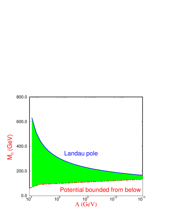
Figure 4: Theoretical limits on the Higgs boson mass. The allowed region is shaded. The region above the solid line (labelled Landau pole) is forbidden because the quartic coupling is infinite. The region below the dot-dash line is forbidden because the quartic coupling is negative, causing the potential to be unbounded from below.

3.3 Bounds from Electroweak Radiative Corrections

The Higgs boson enters into one loop radiative corrections in the Standard Model and so precision electroweak measurements can bound the Higgs boson mass. For example, the $\rho$ parameter gets a contribution from the Higgs boson$\!{}^{{\bf?}}$

$$\rho=1-{11g^{2}\over 96\pi^{2}}\tan^{2}\theta_{W}\log\biggl{(}{M_{h}\over M_{W}}\biggr{)}.$$ (61)

Since the dependence on the Higgs boson mass is only logarithmic, the limits derived on the Higgs boson from this method are relatively weak. In contrast, the top quark contributes quadratically to many electroweak observables such as the $\rho$ parameter.

It is straightforward to demonstrate that at one loop all electroweak parameters have at most a logarithmic dependance on $M_{h}$.$\!{}^{{\bf?}}$ This fact has been glorified by the name of the “screening theorem”.$\!{}^{{\bf?}}$ In general, electroweak radiative corrections involving the Higgs boson take the form,

$$g^{2}\biggl{(}\log{M_{h}\over M_{W}}+g^{2}{M_{h}^{2}\over M_{W}^{2}}\cdots\biggr{)}.$$ (62)

That is, effects quadratic in the Higgs boson mass are always screened by an additional power of $g$ relative to the lower order logarithmic effects and so radiative corrections involving the Higgs boson can never be large.$\!{}^{{\bf?}}$

From precision measurements at LEP and SLC of electroweak observables, the direct measurements of $M_{W}$ and $M_{t}$ at the Tevatron, and the measurements of $\nu$ scattering experiments, there is the bound on the Higgs boson mass coming from the effect of radiative corrections,$\!{}^{{\bf?}}$

$$M_{h}<280~{}GeV\quad(95\%~{}{\rm~{}confidence~{}level}).$$ (63)

This bound does not include the Higgs boson direct search experiments and applies only in the minimal Standard Model. Since the bound of Eq. 63 arises from loop corrections, it can be circumvented by unknown new physics which contributes to the loop corrections.

The relationship between $M_{W}$ and $M_{t}$ arising from radiative corrections depends sensitively on the Higgs boson mass. The radiative corrections to $M_{W}$ can be written as,

$$\biggl{(}{M_{W}^{2}\over M_{Z}^{2}}\biggr{)}=1-{\pi\alpha\over\sqrt{2}G_{F}M_{W}^{2}(1-\delta r)}\quad,$$ (64)

where $\delta r$ is a function of $M_{t}^{2}$ and $\log(M_{h})$. The results using the Tevatron measurements of $M_{W}$ and $M_{t}$ are shown in Fig. 5 and clearly prefer a relatively light Higgs boson, in agreement with the global fit of Eq. 63.

While the Higgs boson mass remains a free parameter, the combination of limits from electroweak radiative corrections and the triviality bounds of the previous section suggest that the Higgs boson may be relatively light, in the few hundred GeV range.

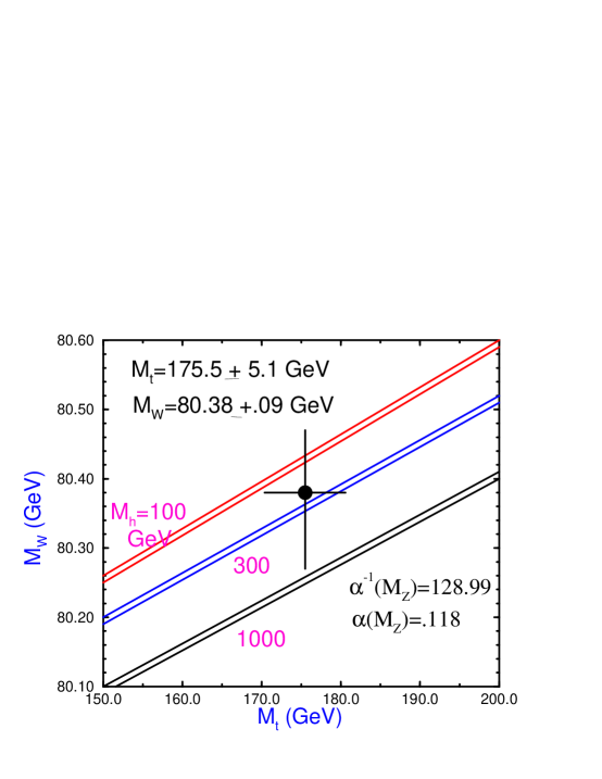
Figure 5: Limits on the Higgs boson mass from the Tevatron measurements of $M_{W}$ and $M_{t}$ for various values of the Higgs boson mass.

4 Higgs Branching Ratios

In the Higgs sector, the Standard Model is extremely predictive, with all couplings, decay widths, and production cross sections given in terms of the unknown Higgs boson mass. The measurements of the various Higgs decay channels will serve to discriminate between the Standard Model and other models with more complicated Higgs sectors which may have different decay chains and Yukawa couplings. It is hence vital that we have reliable predictions for the branching ratios in order to verify the correctness of the Yukawa couplings of the Standard Model.$\!{}^{{\bf?}}$

In this section, we review the Higgs boson branching ratios in the Standard Model.

4.1 Decays to Fermion Pairs

The dominant decays of a Higgs boson with a mass below the $W^{+}W^{-}$ threshold are into fermion- antifermion pairs. In the Born approximation, the width into charged lepton pairs is

$$\Gamma(h\rightarrow l^{+}l^{-})={G_{F}M_{l}^{2}\over 4\sqrt{2}\pi}M_{h}\beta_{l}^{3}\quad,$$ (65)

where $\beta_{l}\equiv\sqrt{1-4M_{l}^{2}/M_{h}^{2}}$ is the velocity of the final state leptons. The Higgs boson decay into quarks is enhanced by the color factor $N_{c}=3$ and also receives significant QCD corrections,

$$\Gamma(h\rightarrow q{\overline{q}})={3G_{F}M_{q}^{2}\over 4\sqrt{2}\pi}M_{h}\beta_{q}^{3}\biggl{(}1+{4\over 3}{\alpha_{s}\over\pi}\Delta_{h}^{QCD}\biggr{)}\quad,$$ (66)

where the QCD correction factor, $\Delta_{h}^{QCD}$, can be found in Ref. 22. The Higgs boson clearly decays predominantly into the heaviest fermion kinematically allowed.

A large portion of the QCD corrections can be absorbed by expressing the decay width in terms of a running quark mass, $M_{q}(\mu)$, evaluated at the scale $\mu=M_{h}$. The QCD corrected decay width can then be written as,$\!{}^{{\bf?}}$

$$\Gamma(h\rightarrow q{\overline{q}})={3G_{F}\over 4\sqrt{2}\pi}M_{q}^{2}(M_{h}^{2})M_{h}\beta_{q}^{3}\biggl{(}1+5.67{\alpha_{s}(M_{h}^{2})\over\pi}+\cdots\biggr{)},$$ (67)

where $\alpha_{s}(M_{h}^{2})$ is defined in the ${\overline{MS}}$ scheme with $5$ flavors and $\Lambda_{\overline{MS}}=150~{}GeV$. The ${\cal O}(\alpha_{s}^{2})$ corrections are also known in the limit $M_{h}>>M_{q}$.$\!{}^{{\bf?}}$

For $10~{}GeV<M_{h}<160~{}GeV$, the most important fermion decay mode is $h\rightarrow b{\overline{b}}$. In leading log QCD, the running of the $b$ quark mass is,

$$M_{b}(\mu^{2})=M\biggl{[}{\alpha_{s}(M^{2})\over\alpha_{s}(\mu^{2})}\biggr{]}^{(-12/23)}\biggl{\{}1+{\cal O}(\alpha_{s}^{2})\biggr{\}},$$ (68)

where $M_{b}(M^{2})\equiv M$ implies that the running mass at the position of the propagator pole is equal to the location of the pole. For $M_{b}(M_{b}^{2})=4.2~{}GeV$, this yields an effective value $M_{b}((M_{h}=100~{}GeV)^{2})=3~{}GeV$. Inserting the QCD corrected mass into the expression for the width thus leads to a significantly smaller rate than that found using $M_{b}=4.2~{}GeV$. For a Higgs boson in the $100~{}GeV$ range, the ${\cal O}(\alpha_{s})$ corrections decrease the decay width for $h\rightarrow b{\overline{b}}$ by about a factor of two.

The electroweak radiative corrections to $h\rightarrow q{\overline{q}}$ are not significant and amount to only a few percent correction.$\!{}^{{\bf?}}$ These can be neglected in comparison with the much larger QCD corrections.

The branching ratios for the dominant decays to fermion- antifermion pairs are shown in Fig. 6. The decrease in the $h\rightarrow f{\overline{f}}$ branching ratios at $M_{h}\sim 150~{}GeV$ is due to the turn-on of the $WW^{*}$ decay channel, where $W^{*}$ denotes a virtual $W$. For most of the region below the $W^{+}W^{-}$ threshold, the Higgs decays almost entirely to $b{\overline{b}}$ pairs, although it is possible that the decays to $\tau^{+}\tau^{-}$ will be useful in the experimental searches. The other fermionic Higgs boson decay channels are almost certainly too small to be separated from the backgrounds.

Even including the QCD corrections, the rates roughly scale with the fermion masses and the color factor, $N_{c}$,

$${\Gamma(h\rightarrow b{\overline{b}})\over\Gamma(h\rightarrow\tau^{+}\tau^{-})}\sim{3M_{b}^{2}(M_{h}^{2})\over M_{\tau}^{2}},$$ (69)

and so a measurement of the branching ratios could serve to verify the correctness of the Standard Model couplings. The largest uncertainty is in the value of $\alpha_{s}$, which affects the running $b$ quark mass, as in Eq. 68 .

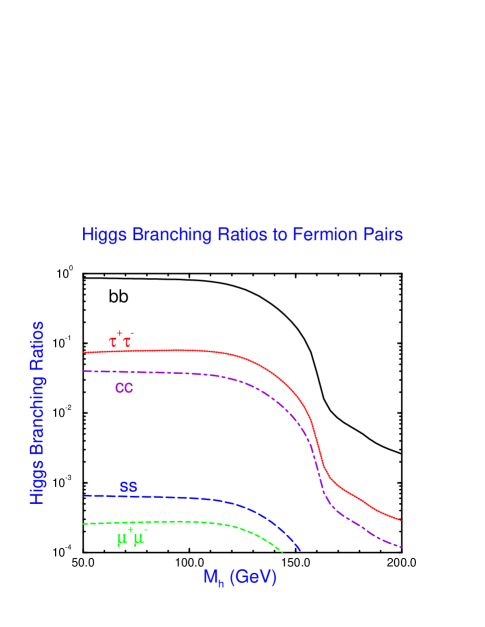
Figure 6: Branching ratios of the Standard Model Higgs boson to fermion-antifermion pairs, including QCD radiative corrections. The radiative corrections were computed using the program HDECAY.²⁵

4.2 Decays to Gauge Boson Pairs

The Higgs boson can also decay to gauge boson pairs. At tree level, the decays $h\rightarrow W^{+}W^{-}$ and $h\rightarrow ZZ$ are possible, while at one-loop the decays $h\rightarrow gg,\gamma\gamma,~{}\gamma Z$ occur.

The decay widths of the Higgs boson to physical $W^{+}W^{-}$ or $ZZ$ pairs are given by,

$$\Gamma(h\rightarrow W^{+}W^{-})= {G_{F}M_{h}^{3}\over 8\pi\sqrt{2}}\sqrt{1-r_{W}}(1-r_{W}+{3\over 4}r_{W}^{2})$$

$$\Gamma(h\rightarrow ZZ)= {G_{F}M_{h}^{3}\over 16\pi\sqrt{2}}\sqrt{1-r_{Z}}(1-r_{Z}+{3\over 4}r_{Z}^{2}),$$ (70)

where $r_{V}\equiv 4M_{V}^{2}/M_{h}^{2}$.

Below the $W^{+}W^{-}$ and $ZZ$ thresholds, the Higgs boson can also decay to vector boson pairs $VV^{*}$, ($V=W^{\pm},Z$), with one of the gauge bosons off-shell. The widths, summed over all available channels for $V^{*}\rightarrow f{\overline{f}}$ are:  $\!{}^{{\bf?}}$

$$\Gamma(h\rightarrow ZZ^{*}) = {g^{4}M_{h}\over 2048(1-s_{W})^{2}\pi^{3}}\biggl{(}7-{40\over 3}s_{W}+{160\over 9}s_{W}^{2}\biggr{)}F\biggl{(}{M_{Z}\over M_{h}}\biggr{)}$$

$$\Gamma(h\rightarrow WW^{*}) = {3g^{4}M_{h}\over 512\pi^{3}}F\biggl{(}{M_{W}\over M_{h}}\biggr{)}\quad,$$ (71)

where $s_{W}\equiv\sin^{2}\theta_{W}$ and

$$F(x) \equiv -\mid 1-x^{2}\mid\biggl{(}{47\over 2}x^{2}-{13\over 2}+{1\over x^{2}}\biggr{)}-3\biggl{(}1-6x^{2}+4x^{4}\biggr{)}\mid\ln(x)\mid$$ (72)

$$+3{1-8x^{2}+20x^{4}\over\sqrt{4x^{2}-1}}\cos^{-1}\biggl{(}{3x^{2}-1\over 2x^{3}}\biggr{)}\quad.$$

These widths can be significant when the Higgs boson mass approaches the real $W^{+}W^{-}$ and $ZZ$ thresholds, as can be seen in Fig. 7. The $WW^{*}$ and $ZZ^{*}$ branching ratios grow rapidly with increasing Higgs mass and above $2M_{W}$ the rate for $h\rightarrow W^{+}W^{-}$ is close to 1. The decay width to $ZZ^{*}$ is roughly an order of magnitude smaller than the decay width to $WW^{*}$ over most of the Higgs mass range due to the smallness of the neutral current couplings as compared to the charged current couplings.

The decay of the Higgs boson to gluons arises through fermion loops,$\!{}^{{\bf?}}$

$$\Gamma_{0}(h\rightarrow gg)={G_{F}\alpha_{s}^{2}M_{h}^{3}\over 64\sqrt{2}\pi^{3}}\mid\sum_{q}F_{1/2}(\tau_{q})\mid^{2}$$ (73)

where $\tau_{q}\equiv 4M_{q}^{2}/M_{h}^{2}$ and $F_{1/2}(\tau_{q})$ is defined to be,

$$F_{1/2}(\tau_{q})\equiv-2\tau_{q}\biggl{[}1+(1-\tau_{q})f(\tau_{q})\biggr{]}\quad.$$ (74)

The function $f(\tau_{q})$ is given by,

$$f(\tau_{q})=\left\{\begin{array}[]{ll}\biggl{[}\sin^{-1}\biggl{(}\sqrt{1/\tau_{q}}\biggr{)}\biggr{]}^{2},&\hbox{if~{}}\tau_{q}\geq 1\\ -{1\over 4}\biggl{[}\log\biggl{(}{x_{+}\over x_{-}}\biggr{)}-i\pi\biggr{]}^{2},&\hbox{ if~{}}\tau_{q}<1,\end{array}\right.$$ (75)

with

$$x_{\pm}=1\pm\sqrt{1-\tau_{q}}.$$ (76)

In the limit in which the quark mass is much less than the Higgs boson mass, (the relevant limit for the $b$ quark),

$$F_{1/2}\rightarrow{2M_{q}^{2}\over M_{h}^{2}}\log^{2}\biggl{(}{M_{q}\over M_{h}}\biggr{)}.$$ (77)

A Higgs boson decaying to $b{\overline{b}}$ will therefore be extremely narrow. On the other hand, for a heavy quark, $\tau_{q}\rightarrow\infty$, and $F_{1/2}(\tau_{q})$ approaches a constant,

$$F_{1/2}\rightarrow-{4\over 3}.$$ (78)

It is clear that the dominant contribution to the gluonic decay of the Higgs boson is from the top quark loop and from possible new generations of heavy fermions. A measurement of this rate would serve to count the number of heavy fermions since the effects of the heavy fermions do not decouple from the theory.

The QCD radiative corrections from $h\rightarrow ggg$ and $h\rightarrow gq{\overline{q}}$ to the hadronic decay of the Higgs boson are large and they typically increase the width by more than $50\%$. The radiatively corrected width can be approximated by

$$\Gamma(h\rightarrow ggX)=\Gamma_{0}(h\rightarrow gg)\biggl{[}1+C{\alpha_{s}(\mu)\over\pi}\biggr{]}\quad,$$ (79)

where $C={215\over 12}-{23\over 6}\log(\mu^{2}/M_{h}^{2})$, for $M_{h}<2M_{t}$.$\!{}^{{\bf?}}$ The radiatively corrected branching ratio for $h\rightarrow ggX$ is the solid curve in Fig. 7.

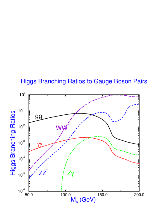
Figure 7: Branching ratios of the Standard Model Higgs boson to gauge boson pairs, including QCD radiative corrections. The rates to $WW^{*}$ and $ZZ^{*}$ must be multiplied by the appropriate branching ratios for $W^{*}$ and $Z^{*}$ decays to $f{\overline{f}}$ pairs. The radiative corrections were computed using the program HDECAY.²⁵

The decay $h\rightarrow Z\gamma$ is not useful phenomenologically, so we will not discuss it here although the complete expression for the branching ratio can be found in Ref. 28. On the other hand, the decay $h\rightarrow\gamma\gamma$ is an important mode for the Higgs search at the LHC. At lowest order, the branching ratio is, $\!{}^{{\bf?}}$

$$\Gamma(h\rightarrow\gamma\gamma)={\alpha^{2}G_{F}\over 128\sqrt{2}\pi^{3}}M_{h}^{3}\mid\sum_{i}N_{ci}Q_{i}^{2}F_{i}(\tau_{i})\mid^{2}$$ (80)

where the sum is over fermions and $W^{\pm}$ bosons with $F_{1/2}(\tau_{q})$ given in Eq. 23, and

$$F_{W}(\tau_{W})=2+3\tau_{W}[1+(2-\tau_{W})f(\tau_{W})]\quad.$$ (81)

$\tau_{W}=4M_{W}^{2}/M_{h}^{2}$, $N_{Ci}=3$ for quarks and $1$ otherwise, and $Q_{i}$ is the electric charge in units of $e$. The function $f(\tau_{q})$ is given in Eq. 75. The $h\rightarrow\gamma\gamma$ decay channel clearly probes the possible existence of heavy charged particles. (Charged scalars, such as those existing in supersymmetric models, would also contribute to the rate.)$\!{}^{{\bf?}}$

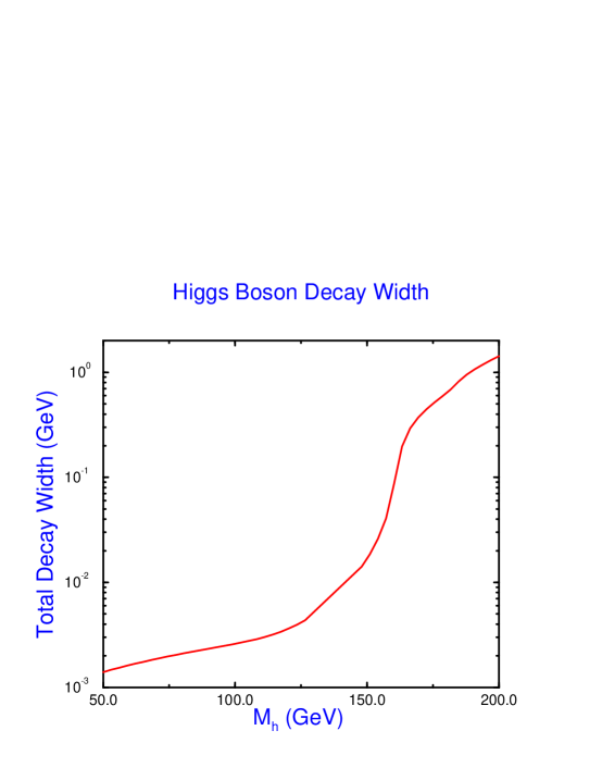
Figure 8: Total Higgs boson decay width in the Standard Model, including QCD radiative corrections. The turn-on of the $W^{+}W^{-}$ threshold at $M_{h}\sim 160~{}GeV$ is obvious.

In the limit where the particle in the loop is much heavier than the Higgs boson, $\tau\rightarrow\infty$,

$$F_{1/2} \rightarrow -{4\over 3}$$

$$F_{W} \rightarrow ~{}7\quad.$$ (82)

The top quark contribution $(F_{1/2})$ is therefore much smaller than that of the $W$ loops $(F_{W})$ and so we expect the QCD corrections to be less important than is the case for the $h\rightarrow gg$ decay. In fact the QCD corrections to the total width for $h\rightarrow\gamma\gamma$ are quite small.$\!{}^{{\bf?}}$ The $h\rightarrow\gamma\gamma$ branching ratio is the dotted line in Fig. 7. For small Higgs masses it rises with increasing $M_{h}$ and peaks at around $2\times 10^{-3}$ for $M_{h}\sim 125~{}GeV$. Above this mass, the $WW^{*}$ and $ZZ^{*}$ decay modes are increasing rapidly with increasing Higgs mass and the $\gamma\gamma$ mode becomes further suppressed.

The total Higgs boson width for a Higgs boson with mass less than $M_{h}\sim 200~{}GeV$ is shown in Fig. 8. As the Higgs boson becomes heavier twice the $W$ boson mass, its width becomes extremely large (see Eq. 122). Below around $M_{h}\sim 150~{}GeV$, the Higgs boson is quite narrow with $\Gamma_{h}<10~{}MeV$. As the $WW^{*}$ and $ZZ^{*}$ channels become accessible, the width increases rapidly with $\Gamma_{h}\sim 1~{}GeV$ at $M_{h}\sim 200~{}GeV$. Below the $W^{+}W^{-}$ threshold, the Higgs boson width is too narrow to be resolved experimentally. The total width for the lightest neutral Higgs boson in the minimal supersymmetric model is typically much smaller than the Standard Model width for the same Higgs boson mass and so a measurement of the total width could serve to discriminate between the two models.

5 Higgs Production at LEP and LEP2

Since the Higgs boson coupling to the electron is very small, $\sim m_{e}/v$, the $s-$channel production mechanism, $e^{+}e^{-}\rightarrow h$, is minute and the dominant Higgs boson production mechanism at LEP and LEP2 is the associated production with a $Z$, $e^{+}e^{-}\rightarrow Z^{*}\rightarrow Zh$, as shown in Fig. 9.

Figure 9: Higgs production through $e^{+}e^{-}\rightarrow Zh$.

At LEP2, a physical $Z$ boson can be produced and the cross section is,$\!{}^{{\bf?}}$

$${\hat{\sigma}}(e^{+}e^{-}\rightarrow Zh)={\pi\alpha^{2}\lambda_{Zh}^{1/2}[\lambda_{Zh}+12{M_{Z}^{2}\over s}][1+(1-4\sin^{2}\theta_{W})^{2}]\over 192s\sin^{4}\theta_{W}\cos^{4}\theta_{W}(1-M_{Z}^{2}/s)^{2}}$$ (83)

where

$$\lambda_{Zh}\equiv(1-{M_{h}^{2}+M_{Z}^{2}\over s})^{2}-{4M_{h}^{2}M_{Z}^{2}\over s^{2}}\quad.$$ (84)

The center of mass momentum of the produced $Z$ is $\lambda_{Zh}^{1/2}\sqrt{s}/2$ and the cross section is shown in Fig. 10 as a function of $\sqrt{s}$ for different values of the Higgs boson mass. The cross section peaks at $\sqrt{s}\sim M_{Z}+2M_{h}$. From Fig. 10, it is apparent that the cross section increases rapidly with increasing energy and so the best limits on the Higgs boson mass will be obtained at the highest energy.

The electroweak radiative corrections are quite small at LEP2 energies.$\!{}^{{\bf?}}$ Photon bremsstrahlung can be important, however, since it is enhanced by a large logarithm, $\log(s/m_{e}^{2})$. The photon radiation can be accounted for by integrating the Born cross section of Eq. 83 with a radiator function $F$ which includes virtual and soft photon effects, along with hard photon radiation,$\!{}^{{\bf?}}$

$$\sigma={1\over s}\int ds^{\prime}F(x,s){\hat{\sigma}}(s^{\prime})$$ (85)

where $x=1-s^{\prime}/s$ and the radiator function $F(x,s)$ is known to ${\cal O}(\alpha^{2})$, along with the exponentiation of the infrared contribution,

$$F(x,s) = tx^{t-1}\biggl{\{}1+{3\over 4}t\biggr{\}}+\biggl{\{}{x\over 2}-1\biggr{\}}t+{\cal O}(t^{2})$$

$$t \equiv {2\alpha\over\pi}\biggl{[}\log\biggl{(}{s\over m_{e}^{2}}\biggr{)}-1\biggr{]}\quad.$$ (86)

Photon radiation significantly reduces the $Zh$ production rate from the Born cross section as shown in Fig. 11.

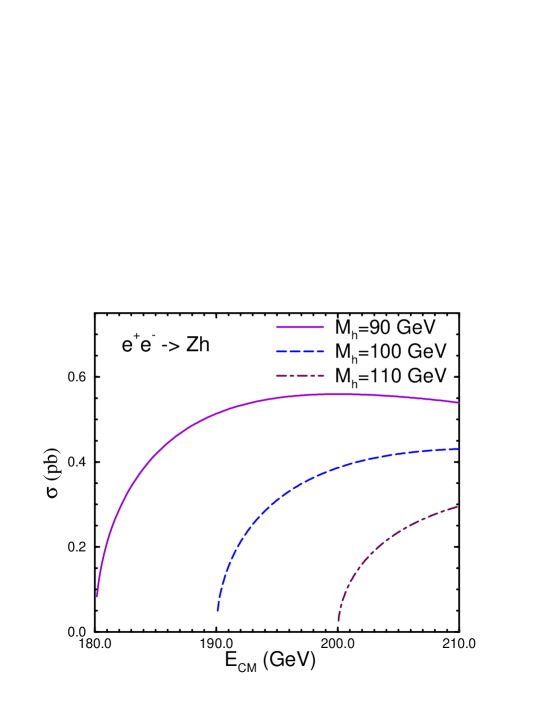
Figure 10: Born cross section for $e^{+}e^{-}\rightarrow Zh$ as a function of center of mass energy.

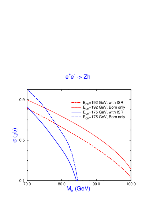
Figure 11: Effects of initial state radiation(ISR) on the process $e^{+}e^{-}\rightarrow Zh$. The curves labelled “Born only” are the results of Eq. 83, while those labelled “with ISR” include the photon radiation as in Eq. 85.

A Higgs boson which can be produced at LEP or LEP2 will decay mostly to $b{\overline{b}}$ pairs, so the final state from $e^{+}e^{-}\rightarrow Zh$ will have four fermions. The dominant background is $Zb{\overline{b}}$ production, which can be efficiently eliminated by $b$-tagging almost up to the kinematic limit for producing the Higgs boson. LEP2 studies estimate that with $\sqrt{s}=200~{}GeV$ and ${\cal L}=100~{}pb^{-1}$ per experiment, a Higgs boson mass of $107~{}GeV$ could be observed at the $5\sigma$ level.$\!{}^{{\bf?}}$ A higher energy $e^{+}e^{-}$ machine (such as an NLC with $\sqrt{s}\sim 500~{}GeV$) could push the Higgs mass limit to around $M_{h}\sim.7\sqrt{s}$.

Currently the highest energy data at LEP2 is $\sqrt{s}=183~{}GeV$. The combined limit from the four LEP2 detectors is$\!{}^{{\bf?}}$

$$M_{h}>89.8~{}GeV\quad\quad{\hbox{at~{}95\%~{}c.l.}}$$ (87)

This limit includes both hadronic and leptonic decay modes of the $Z$. Note how close the result is to the kinematic boundary.

The cross section for $e^{+}e^{-}\rightarrow Zh$ is $s$-wave and so has a very steep dependence on energy and on the Higgs boson mass at threshold, as is clear from Fig. 10. This makes possible a precision measurement of the Higgs mass. By measuring the cross section at threshold and normalizing to a second measurement above threshold in order to minimize systematic uncertainties a high energy $e^{+}e^{-}$ collider with $\sqrt{s}=500~{}GeV$ could obtain a $1\sigma$ measurement of the mass $\!{}^{{\bf?}}$

$$\Delta M_{h}\sim 60~{}MeV\sqrt{{100fb^{-1}\over L}}\quad\quad{\rm for~{}~{}}M_{h}=100~{}GeV\quad,$$ (88)

where $L$ is the total integrated luminosity. The precision becomes worse for larger $M_{h}$ because of the decrease in the signal cross section. (Note that the luminosity at LEP2 will not be high enough to perform this measurement.)

The angular distribution of the Higgs boson from the $e^{+}e^{-}\rightarrow Zh$ process is

$${1\over\sigma}{d\sigma\over d\cos\theta}\sim\lambda_{Zh}^{2}\sin^{2}\theta+{8M_{Z}^{2}\over s}$$ (89)

so that at high energy the distribution is that of a scalar particle,

$${1\over\sigma}{d\sigma\over d\cos\theta}\sim\sin^{2}\theta\quad.$$ (90)

If the Higgs boson were CP odd, on the other hand, the angular distribution would be $1+\cos^{2}\theta$. Hence the angular distribution is sensitive to the spin-parity assignments of the Higgs boson.$\!{}^{{\bf?}}$ The angular distribution of this process is also quite sensitive to non-Standard Model $ZZh$ couplings.$\!{}^{{\bf?}}$

6 Higgs Production in Hadronic Collisions

We turn now to the production of the Higgs boson in $pp$ and $p\overline{p}$ collisions.

6.1 Gluon Fusion

Since the coupling of a Higgs boson to an up quark or a down quark is proportional to the quark mass, this coupling is very small. The primary production mechanism for a Higgs boson in hadronic collisions is through gluon fusion, $gg\rightarrow h$, which is shown in Fig. 12.$\!{}^{{\bf?}}$ The loop contains all quarks in the theory and is the dominant contribution to Higgs boson production at the LHC for all $M_{h}<1~{}TeV$. (In extensions of the standard model, all massive colored particles run in the loop.)

Figure 12: Higgs boson production through gluon fusion with a quark loop.

The lowest order cross section for $gg\rightarrow h$ is,$\!{}^{{\bf?},{\bf?}}$

$${\hat{\sigma}}(gg\rightarrow h) = {\alpha_{s}^{2}\over 1024\pi v^{2}}\mid\sum_{q}F_{1/2}(\tau_{q})\mid^{2}\delta\biggl{(}1-{{\hat{s}}\over M_{h}^{2}}\biggr{)}$$ (91)

$$\equiv {\hat{\sigma}}_{0}(gg\rightarrow h)\delta\biggl{(}1-{{\hat{s}}\over M_{h}^{2}}\biggr{)}\quad,$$

where ${\hat{s}}$ is the gluon-gluon sub-process center of mass energy, $v=246~{}GeV$, and $F_{1/2}(\tau_{q})$ is defined in Eq. 74. In the heavy quark limit, $(M_{t}/M_{h}\rightarrow\infty)$, the cross section becomes a constant,

$${\hat{\sigma}}_{0}(gg\rightarrow h)\sim{\alpha_{s}^{2}\over 576\pi v^{2}}\quad.$$ (92)

Just like the decay process, $h\rightarrow gg$, this rate counts the number of heavy quarks and so could be a window into a possible fourth generation of quarks.

The Higgs boson production cross section at a hadron collider can be found by integrating the parton cross section, $\sigma_{0}(pp\rightarrow h)$, with the gluon structure functions, $g(x)$,

$$\sigma_{0}(pp\rightarrow h)={\hat{\sigma}_{0}}\tau\int_{\tau}^{1}{dx\over x}g(x)g\biggl{(}{\tau\over x}\biggr{)},$$ (93)

where $\sigma_{0}$ is given in Eq. 91, $\tau\equiv M_{h}^{2}/S$, and $S$ is the hadronic center of mass energy.

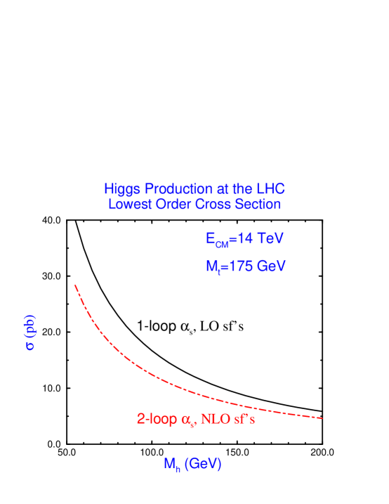
Figure 13: Cross section for gluon fusion, $gg\rightarrow h$, at the LHC using the lowest order parton cross section of Eq. 91. The solid (dot-dashed) line uses the one-loop (two-loop) expression for $\alpha_{s}(\mu)$, along with structure functions fitted to lowest order (next to lowest order) expressions for the data. The renormalization scale is $\mu=M_{h}$.

We show the rate obtained using the lowest order parton cross section of Eq. 91 in Fig. 13 for the LHC. When computing the lowest order result from Eq. 91, it is ambiguous whether to use the one- or two- loop result for $\alpha_{s}(\mu)$ and which structure functions to use; a set fit to data using only the lowest order in $\alpha_{s}$ predictions or a set which includes some higher order effects. The difference between the equations for $\alpha_{s}$ and the different structure functions is ${\cal O}(\alpha_{s}^{2})$ and hence higher order in $\alpha_{s}$ when one is computing the “lowest order” result. In Fig. 13, we show two different definitions of the lowest order result and see that they differ significantly from each other. We will see in the next section that the result obtained using the $2$-loop $\alpha_{s}$ and NLO structure functions, but the lowest order parton cross section, is a poor approximation to the radiatively corrected rate. Fig. 13 takes the scale factor $\mu=M_{h}$ and the results are quite sensitive to this choice.

6.2 QCD Corrections to $gg\rightarrow h$

In order to obtain reliable predictions for the production rate, it is important to compute the $2-$loop QCD radiative corrections to $gg\rightarrow h$. The complete ${\cal O}(\alpha_{s}^{3})$ calculation is available in Ref 39. The analytic result is quite complicated, but the computer code including all QCD radiative corrections is readily available.

The result in the $M_{h}/M_{t}\rightarrow 0$ limit turns out to be an excellent approximation to the exact result for the 2-loop corrected rate for $gg\rightarrow h$ and can be used in most cases. The heavy quark limit can be obtained from the gauge invariant effective Lagrangian,$\!{}^{{\bf?},{\bf?}}$

$${\cal L}=-{1\over 4}\biggl{[}1-{2\beta_{s}\over g_{s}(1+\delta)}{h\over v}\biggr{]}G_{\mu\nu}^{A}G^{A\mu\nu}-{M_{t}\over v}{\overline{t}}th\quad,$$ (94)

where $\delta=2\alpha_{s}/\pi$ is the anomalous mass dimension arising from the renormalization of the $t{\overline{t}}h$ Yukawa coupling constant, $g_{s}$ is the QCD coupling constant, and $G_{\mu\nu}^{A}$ is the color $SU(3)$ field. This Lagrangian can be derived using low energy theorems which are valid in the limit $M_{h}<<M_{t}$ and yields momentum dependent $ggh$, $gggh$, and $ggggh$ vertices which can be used to compute the rate for $gg\rightarrow h$ to ${\cal O}(\alpha_{s}^{3})$.$\!{}^{{\bf?}}$

Since the $hgg$ coupling in the $M_{t}\rightarrow\infty$ limit results from heavy fermion loops, it is only the heavy fermions which contribute to $\beta_{s}$ in Eq. 94. To ${\cal O}(\alpha_{s}^{2})$, the heavy fermion contribution to the QCD $\beta$ function is,

$${\beta_{s}\over g_{s}}\mid{\rm heavy~{}fermions}=N_{H}{\alpha_{s}\over 6\pi}\biggl{[}1+{19\alpha_{s}\over 4}\biggr{]}\quad,$$ (95)

where $N_{H}$ is the number of heavy fermions.

The parton level cross section for $gg\rightarrow h$ is found by computing the ${\cal O}(\alpha_{s}^{3})$ virtual graphs for $gg\rightarrow h$ and combining them with the bremsstrahlung process $gg\rightarrow gh$. The answer in the heavy top quark limit is,$\!{}^{{\bf?},{\bf?}}$

$${\hat{\sigma}}_{1}(gg\rightarrow hX)={\alpha_{s}^{2}(\mu)\over 576\pi v^{2}}\biggl{\{}\delta(1-z)+{\alpha_{s}(\mu)\over\pi}\biggl{[}h(z)+{\bar{h}}(z)\log\biggl{(}{M_{h}^{2}\over\mu^{2}}\biggr{)}\biggr{]}\biggr{\}}$$ (96)

where

$$h(z) = \delta(1-z)\biggl{(}\pi^{2}+{11\over 2}\biggr{)}-{11\over 2}(1-z)^{3}$$

$$+6\biggl{(}1+z^{4}+(1-z)^{4}\biggr{)}\biggl{(}{\log(1-z)\over 1-z}\biggr{)}_{+}-{\overline{h}}(z)\log(z)$$

$${\bar{h}}(z) = 6\biggl{(}{z^{2}\over(1-z)_{+}}+(1-z)+z^{2}(1-z)\biggr{)}$$ (97)

and $z\equiv M_{h}^{2}/{\hat{s}}$. The answer is written in terms of “+” distributions, which are defined by the integrals,

$$\int_{0}^{1}{f(x)\over(1-x)_{+}}\equiv\int^{1}_{0}{f(x)-f(1)\over 1-x}\quad.$$ (98)

The factor $\mu$ is an arbitrary renormalization point. To $\alpha_{s}^{3}$, the physical hadronic cross section is independent of $\mu$. There are also ${\cal O}(\alpha_{s}^{3})$ contributions from $q{\overline{q}}$, $qg$ and ${\overline{q}}g$ initial states, but these are numerically small.

We can define a $K$ factor as

$$K\equiv{{\sigma}_{1}(pp\rightarrow hX)\over{\sigma}_{0}(pp\rightarrow h)}\quad,$$ (99)

where $\sigma_{1}(pp\rightarrow hX)$ is the ${\cal O}(\alpha_{s}^{3})$ radiatively corrected rate for Higgs production and $\sigma_{0}$ is the lowest order rate found from Eq. 91. From Eq. 97, it is apparent that a significant portion of the corrections result from the rescaling of the lowest order result,

$$K\sim 1+{\alpha_{s}(\mu)\over\pi}\biggl{[}\pi^{2}+{11\over 2}+\cdots\biggr{]}\quad.$$ (100)

Of course $K$ is not a constant, but depends on the renormalization scale $\mu$ as well as $M_{h}$. The radiatively corrected cross section ${\hat{\sigma}}_{1}$ should be convoluted with next-to-leading order structure functions, while it is ambiguous which structure functions and definition of $\alpha_{s}$ to use in defining the lowest order result, ${\hat{\sigma}}_{0}$, as discussed above.

The $K$ factor varies between $2$ and $3$ at the LHC and so the QCD corrections significantly increase the rate from the lowest order result. The heavy top quark limit is an excellent approximation to the $K$ factor. The easiest way to compute the radiatively corrected cross section is therefore to calculate the lowest order cross section including the complete mass dependence of Eq. 91 and then to multiply by the $K$ factor computed in the $M_{t}\rightarrow\infty$ limit. This result will be extremely accurate.

The other potentially important correction to the $hgg$ coupling is the two-loop electroweak contribution involving the top quark, which is of ${\cal O}(\alpha_{S}G_{F}M_{t}^{2})$. In the heavy quark limit, the function $F_{1/2}(\tau_{q})$ of Eq. 74 receives a contribution, $\!{}^{{\bf?}}$

$$F_{1/2}(\tau_{q})\rightarrow F_{1/2}(\tau_{q})\biggl{(}1+{G_{F}M_{t}^{2}\over 16\sqrt{2}\pi^{2}}\biggr{)}\quad.$$ (101)

When the total rate for Higgs production is computed, the ${\cal O}(\alpha_{s}G_{F}M_{t}^{2})$ contribution is $<.2\%$ and so can be neglected. The ${\cal O}(\alpha_{s}G_{F}M_{t}^{2})$ contributions therefore do not spoil the usefulness of the $gg\rightarrow h$ mechanism as a means of counting heavy quarks.

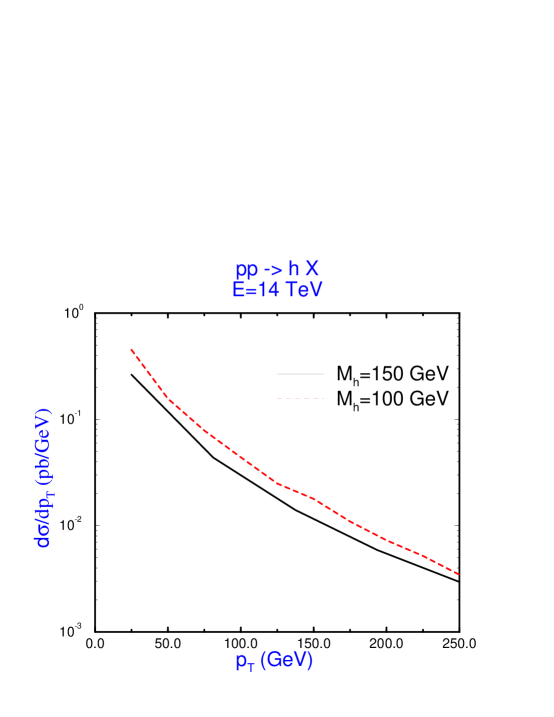
Figure 14: Higgs boson transverse momentum distribution from Eq. 102.

At lowest order the gluon fusion process yields a Higgs boson with no transverse momentum. At the next order in perturbation theory, gluon fusion produces a Higgs boson with finite $p_{T}$, primarily through the process $gg\rightarrow gh$. At low $p_{T}$, the parton cross section diverges as $1/p_{T}^{2}$,$\!{}^{{\bf?}}$

$${d{\hat{\sigma}}\over d{\hat{t}}}(gg\rightarrow gh) = {\hat{\sigma}}_{0}{3\alpha_{s}\over 2\pi}\biggl{\{}{1\over p_{T}^{2}}\biggl{[}\biggl{(}1-{M_{h}^{2}\over{\hat{s}}}\biggr{)}^{4}+1+\biggl{(}{M_{h}^{2}\over{\hat{s}}}\biggr{)}^{4}\biggr{]}$$ (102)

$$-{4\over{\hat{s}}}\biggl{(}1-{M_{h}^{2}\over{\hat{s}}}\biggr{)}^{2}+{2p_{T}^{2}\over{\hat{s}}}\biggr{\}}\quad.$$

The hadronic cross section can be found by integrating Eq. 102 with the gluon structure functions. In Fig. 14, we show the $p_{T}$ spectrum of the Higgs boson at ${\cal O}(\alpha_{s}^{3})$. At the LHC, the event rate even at large $p_{T}$ is significant. This figure clearly demonstrates the singularity at $p_{T}\rightarrow 0$.

6.3 Finding the Higgs Boson at the LHC

We turn now to a discussion of search techniques for the Higgs boson at the LHC. For $M_{h}<1~{}TeV$, gluon fusion is the primary production mechanism.

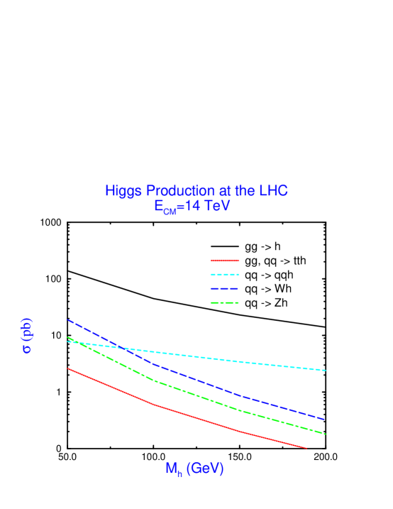
Figure 15: Processes contributing to Higgs production at the LHC.

Fig. 15 shows the Higgs boson production rates from various processes at the LHC. At the present time, there are two large detectors planned for the LHC; the ATLAS detector$\!{}^{{\bf?}}$ and the CMS detector$\!{}^{{\bf?}}$. A more detailed discussion of the experimental issues involved in searching for the Higgs boson at the LHC can be found in the 1997 TASI lectures of F.  Paige.$\!{}^{{\bf?}}$

The production rate for the Higgs boson at the LHC is significant, $\sigma_{h}\sim 10~{}pb$ for $M_{h}\sim 200~{}GeV$. However, in order to see the Higgs boson it must decay into some channel where it is not overwhelmed by the background. For $M_{h}<2M_{W}$ the Higgs boson decays predominantly to $b{\overline{b}}$ pairs. Unfortunately, the QCD production of $b$ quarks is many orders of magnitude larger than Higgs production and so this channel is thought to be useless.$\!{}^{{\bf?}}$ One is led to consider rare decay modes of the Higgs boson where the backgrounds may be smaller. The decay channels which have received the most attention are $h\rightarrow\gamma\gamma$ and $h\rightarrow ZZ^{*}$.$\!{}^{{\bf?}}$ The branching ratios for these decays are shown in Fig. 7 and can be seen to be quite small. (The rates for off-shell gauge bosons, $h\rightarrow VV^{*}$, $V=W^{\pm},Z$ must be multiplied by the relevant branching ratios, $V\rightarrow f^{\prime}{\overline{f}}$.)

The $h\rightarrow ZZ^{*}$ decay mode can lead to a final state with $4$ leptons, $2$ of whose mass reconstructs to $M_{Z}$ while the invariant mass of the $4$ lepton system reconstructs to $M_{h}$. The largest background to this decay is $t\overline{t}$ production with $t\rightarrow Wb\rightarrow(l\nu)(cl\nu)$. There are also backgrounds from $Zb\overline{b}$ production, $ZZ^{*}$ production, etc. For $M_{h}=150~{}GeV$, the ATLAS collaboration estimates that there will be 184 signal events and 840 background events in their detector in one year from $h\rightarrow ZZ^{*}\rightarrow(4l)$ with the 4-lepton invariant mass in a mass bin within $\pm 2\sigma$ of $M_{h}$.$\!{}^{{\bf?}}$ The leptons from Higgs decay tend to be more isolated from other particles than those coming from the backgrounds and a series of isolation cuts can be used to reduce the rate to 92 signal and 38 background events. The ATLAS collaboration claims that they will be able to discover the Higgs boson in the $h\rightarrow ZZ^{*}\rightarrow l^{+}l^{-}l^{+}l^{-}$ mode for $130~{}GeV<M_{h}<180~{}GeV$ with an integrated luminosity of $10^{5}~{}pb^{-1}$ (one year of running at the LHC with design luminosity) and using both the electron and muon signatures. For $M_{h}<130~{}GeV$, there are not enough events since the branching ratio is too small (see Fig. 7), while for $M_{h}>180~{}GeV$ the Higgs search can proceed via the $h\rightarrow ZZ$ channel, which we discuss in Section 7.2.

For $M_{h}<130~{}GeV$, the Higgs boson can be searched for through its decay to two photons. The branching ratio in this region is about $10^{-3}$, so for a Higgs boson with $M_{h}\sim 100~{}GeV$ there will be about $3000$ events per year. The Higgs boson decay into the $\gamma\gamma$ channel is an extremely narrow resonance in this region with a width around $1~{}KeV$. From Fig. 7 we see that the branching ratio for $h\rightarrow\gamma\gamma$ falls rapidly with increasing $M_{h}$ and so this decay mode is probably only useful in the region $80~{}GeV<M_{h}<130~{}GeV$.

The irreducible background to $h\rightarrow\gamma\gamma$ comes from $q\overline{q}\rightarrow\gamma\gamma$ and $gg\rightarrow\gamma\gamma$. Extracting the narrow signal from the immense background poses a formidable experimental challenge. The detector must have a mass resolution on the order of $\delta m/m\sim 1.5\%$ in order to be able to hope to observe this signal. For $M_{h}=110~{}GeV$ the ATLAS collaboration estimates that there will be $1430$ signal events and $25,000$ background events in a mass bin equal to the Higgs width. This leads to a ratio ,

$${{\rm Signal}\over\sqrt{{\rm Background}}}\sim 9.$$ (103)

A ratio greater than $5$ is usually ${\it defined}$ as a discovery. ATLAS claims that they will be able to discover the Higgs boson in this channel for $100~{}GeV<M_{h}<130~{}GeV$. (Below $100~{}GeV$ the background is too large and above $130~{}GeV$ the event rate is too small.) Because of its finely grained calorimeter, the CMS collaboration expects to do slightly better.$\!{}^{{\bf?}}$

There are many additional difficult experimental problems associated with the decay channel $h\rightarrow\gamma\gamma$. The most significant of these is the confusion of a photon with a jet. Since the cross section for producing jets is so much larger than that of $h\rightarrow\gamma\gamma$ the experiment must not mistake a photon for a jet more than one time in $10^{4}$. It has not yet been demonstrated that this is experimentally feasible.

One might think that the decay $h\rightarrow\tau^{+}\tau^{-}$ could be measured since as shown in Fig. 6 its branching ratio is considerably larger than $h\rightarrow ZZ^{*}$ and $h\rightarrow\gamma\gamma$; $BR(h\rightarrow\tau^{+}\tau^{-})\sim 3.5\%$ for $M_{h}$ in the $100~{}GeV$ region. The problem is that for the dominant production mechanism, $gg\rightarrow h$, the Higgs boson has no transverse momentum and so the $\tau^{+}\tau^{-}$ invariant mass cannot be reconstructed. If we use the production mechanism $gg\rightarrow hg$, then the Higgs is produced at large transverse momentum and it is possible to reconstruct the $\tau^{+}\tau^{-}$ invariant mass. Unfortunately, the background from $q\overline{q}\rightarrow\tau^{+}\tau^{-}$ and from $t\overline{t}$ decays is much larger than the signal.$\!{}^{{\bf?}}$ Recent studies, however, have shown that the $h\rightarrow\tau^{+}\tau^{-}$ decay channel may be useful at the LHC for $M_{h}\sim~{}110-150~{}GeV$ with $30~{}fb^{-1}$ of data.$\!{}^{{\bf?}}$

6.4 Associated Higgs Boson Production

At the Tevatron and the LHC the process $q{\overline{q}}\rightarrow Wh$ offers the hope of being able to tag the Higgs boson by the $W$ boson decay products.$\!{}^{{\bf?}}$ This process has the rate:

$${\hat{\sigma}}(q_{i}{\overline{q}}_{j}\rightarrow W^{\pm}h)={G_{F}^{2}M_{W}^{6}\mid V_{ij}\mid^{2}\over 6\pi{\hat{s}}^{2}(1-M_{W}^{2}/{\hat{s}})^{2}}\lambda_{Wh}^{1/2}\biggl{[}1+{{\hat{s}}\lambda_{Wh}\over 12M_{W}^{2}}\biggr{]}\quad,$$ (104)

where $\lambda_{Wh}=1-2(M_{W}^{2}+M_{h}^{2})/{\hat{s}}+(M_{W}^{2}-M_{h}^{2})^{2}/{\hat{s}}^{2}$ and $V_{ij}$ is the Kobayashi-Maskawa angle associated with the $q_{i}{\overline{q}}_{j}W$ vertex. This process is sensitive to the $W^{+}W^{-}h$ coupling and so will be different in extensions of the Standard Model.

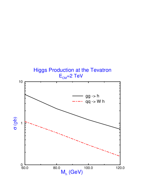
Figure 16: Next to leading order QCD predictions for Higgs boson production at the Tevatron. The dot-dashed line is the $W^{\pm}h$ production rate (summed over $W^{\pm}$ charges), while the solid line is the rate for Higgs production from gluon fusion.

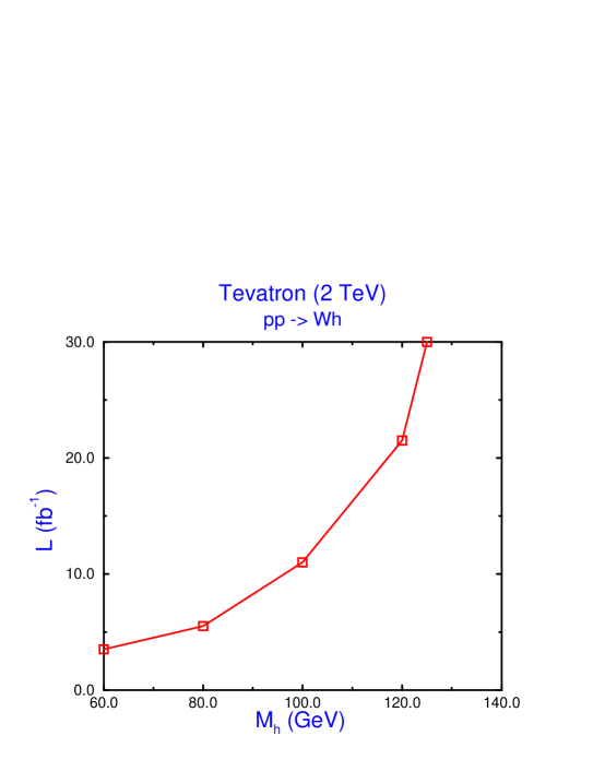
Figure 17: Luminosity required to obtain a $5\sigma$ signal in the process, $p{\overline{p}}\rightarrow Wh,W\rightarrow l\nu,h\rightarrow b{\overline{b}}$ at $\sqrt{s}=2~{}TeV$. From Ref. 54.

Since this mechanism produces a relatively small number of signal events, (as can be seen clearly in Figs. 15 and 16), it is important to compute the rate as accurately as possible by including the QCD radiative corrections. This has been done in Ref. 51, where it is shown that the cross section can be written as

$${d\sigma\over dq^{2}}(pp\rightarrow W^{\pm}h)=\sigma(pp\rightarrow W^{\pm*}){G_{F}M_{W}^{4}\over\sqrt{2}\pi^{2}(q^{2}-M_{W}^{2})^{2}}{\mid{\vec{p}}\mid\over\sqrt{q^{2}}}\biggl{(}1+{\mid{\vec{p}}\mid^{2}\over 3M_{W}^{2}}\biggr{)}$$ (105)

to all orders in $\alpha_{s}$. In Eq. 105, $W^{*}$ is a virtual $W$ with momentum $q$ and $\mid{\vec{p}}\mid=\sqrt{s}\lambda_{Wh}^{1/2}/2$ is the momentum of the outgoing $W^{\pm}$ and $h$. From Eq. 105, it is clear that the radiative corrections to $W^{\pm}h$ production are identical to those for the Drell-Yan process which have been known for some time. Using the DIS factorization scheme, the cross section at the LHC is increased by roughly $17\%$ over the lowest order rate. The QCD corrected cross section is relatively insensitive to the choice of renormalization and factorization scales. It is, however, quite sensitive to the choice of structure functions. The rate for $pp\rightarrow W^{\pm}h$ at the LHC is shown in Fig. 15 (the long-dashed curve) and is more than an order of magnitude smaller than the rate from gluon fusion. The rate for $pp\rightarrow Zh$ is smaller still.

The $Wh$ events can be tagged by identifying the charged lepton from the $W$ decay. Imposing isolation cuts on the lepton significantly reduces the background. At the LHC, there are sufficient events that the Higgs produced in association with a $W$ boson can be identified through the $\gamma\gamma$ decay mode.$\!{}^{{\bf?}}$ ATLAS claims a $4\sigma$ signal in this channel for $80~{}GeV<M_{h}<120~{}GeV$ with $100~{}fb^{-1}$, (this corresponds to about $15$ signal events), while CMS hopes to find a $6-7\sigma$ effect in this channel. There are a large number of $Wh$ events with $W\rightarrow l\nu$ and $h\rightarrow b{\overline{b}}$, but unfortunately the backgrounds to this decay chain are difficult to reject and observation of this signal will probably require a high luminosity.$\!{}^{{\bf?}}$

Associated production of a Higgs boson with a $W^{\pm}$ boson can also potentially be observed at the Tevatron.$\!{}^{{\bf?}}$ For a $100~{}GeV$ Higgs boson, the lowest order cross section is roughly $.2~{}pb$. Including the next-to-leading order corrections increases this to $.3~{}pb$, while summing over the soft gluon effects increases the NLO result by $2-3\%$. $\!{}^{{\bf?}}$ The next to leading order rate for $p{\overline{p}}\rightarrow Wh$ is shown in Fig. 16 and is much smaller that that from gluon fusion. At the Tevatron, the Higgs boson from $W^{\pm}h$ production must be searched for in the $b{\overline{b}}$ decay mode since the $\gamma\gamma$ decay mode produces too few events to be observable. The largest backgrounds are $Wb{\overline{b}}$ and $WZ$, along with top quark production. The background from top quark production is considerably smaller at the Tevatron than at the LHC, however. The Tevatron with $2-4~{}fb^{-1}$ will be sensitive to $M_{h}<M_{Z}$, a region already probed by LEP2.

An upgraded Tevatron with higher luminosity (say $25-30~{}fb^{-1}$) may be able to probe a Higgs boson mass up to about $130~{}GeV$ through the $Wh$ production mechanism.$\!{}^{{\bf?},{\bf?}}$ This result depends critically on the $b$ tagging capabilities of the detectors, since it requires reconstructing the mass of both $b-$ jets. Fig. 17 shows the luminosity required to obtain a $5~{}\sigma$ signal at the Tevatron as a function of Higgs mass. The $120-130~{}GeV$ mass region is particularly important since it is above the kinematic threshold of LEP2 and is the most challenging region to probe at the LHC.

7 Higgs Boson Production from Vector Bosons

7.1 The Effective $W$ Approximation

We turn now to the study of the couplings of the Higgs boson to gauge bosons. We begin by studying the diagram in Fig. 18.

Figure 18: Contribution to heavy Higgs boson production from vector boson scattering.

Naively, one expects this diagram to give a negligible contribution to Higgs production because of the two $W$ boson propagators. However, it turns out that this production mechanism can give an important contribution. The diagram of Fig. 18 can be interpreted in parton model language as the resonant scattering of two $W$ bosons to form a Higgs boson$\!{}^{{\bf?}}$ and we can compute the distribution of $W$ bosons in a quark in an analogous manner to the computation of the distribution of photons in an electron.$\!{}^{{\bf?}}$ By considering the $W$ and $Z$ gauge bosons as partons, calculations involving gauge bosons in the intermediate states can be considerably simplified.

In order to treat the $W^{\pm}$ and $Z$ bosons as partons, we consider them as on-shell physical bosons. We make the approximation that the partons have zero transverse momentum, which ensures that the longitudinal and transverse projections of the $W$ and $Z$ partons are uniquely specified. We want to be able to write a parton level relationship:

$$\sigma(q_{1}+q_{2}\rightarrow q_{1}^{\prime}+X)=\int^{1}_{M_{W}\over E}dxf_{q/W}(x)\sigma(W+q_{2}\rightarrow X).$$ (106)

The function $f_{q/W}(x)$ is called the distribution of $W$’s in a quark and it is defined by Eq. 106. The longitudinal and transverse $W$ distributions in a quark can be found in a manner directly analogous to the derivation of the effective photon approximation,$\!{}^{{\bf?}}$

$$f_{q/W}^{L}(x) = {g^{2}\over 16\pi^{2}}\biggl{(}{1-x\over x}\biggr{)}$$

$$f_{q/W}^{T}(x) = {g^{2}\over 64\pi^{2}x}\log\biggl{(}{4E^{2}\over M_{W}^{2}}\biggr{)}\biggl{[}1+(1-x)^{2}\biggr{]},$$ (107)

where we have averaged over the two transverse polarizations and $E$ is the relevant energy scale of the $WW$ subprocess. The logarithm in Eq. 107 is the same logarithm which appears in the effective photon approximation. The result of Eq. 107 violates our intuition that longitudinal gauge bosons don’t couple to massless fermions. This is because the integral over the angle between the outgoing quark and the emitted $W$ boson picks out the small angle region and hence the subleading term in the $W$ polarization tensor.

It is straightforward to compute the rates for processes involving $WW$ scattering. The hadronic cross section can be written in terms of a luminosity of $W$’s in the proton and a subprocess cross section for the $WW$ scattering,

$$\sigma_{pp\rightarrow WW\rightarrow X}(s)=\int_{\tau_{min}}^{1}d\tau{d{\cal L}\over d\tau}\mid_{pp/WW}\sigma_{WW\rightarrow X}(\tau s)$$ (108)

where the luminosities are defined:

$${d{\cal L}\over d\tau}\mid_{pp/WW} = \sum_{ij}\int_{\tau}^{1}{d\tau^{\prime}\over\tau^{\prime}}\int^{1}_{\tau^{\prime}}{dx\over x}f_{i}(x)f_{j}\biggl{(}{\tau^{\prime}\over x}\biggr{)}{d{\cal L}\over d\zeta}\mid_{q_{i}q_{j}/WW}$$

$${d{\cal L}\over d\tau}\mid_{qq/WW} = \int_{\tau}^{1}{dx\over x}f_{q/W}(x)f_{q/W}\biggl{(}{\tau\over x}\biggr{)}.$$ (109)

$f_{i}(x)$ are the quark distribution functions in the proton and $\zeta\equiv\tau/\tau^{\prime}$. The distributions of $Z$ bosons are found in an identical manner and are roughly a factor of three smaller than the $W$ distributions due to the smaller couplings of the $Z$ to the fermions. The approximation of Eq. 108 has been shown to be extremely accurate for heavy Higgs boson production.

The effective $W$ approximation is particularly useful in models where the electroweak symmetry breaking is due not to the Higgs mechanism, but rather to some strong interaction dynamics (such as in a technicolor model). In these models one typically estimates the strengths of the three and four gauge boson couplings due to the new physics. These interactions can then be folded into the luminosity of gauge bosons to get estimates of the size of the new physics effects.

7.2 Searching for a Heavy Higgs Boson at the LHC

We now have the tools necessary to discuss the search for a very massive Higgs boson. The rates for the various production mechanisms contributing to Higgs production at the LHC are shown in Fig. 15. For $M_{h}<1~{}TeV$ the dominant production mechanism at the LHC is gluon fusion. For heavy Higgs boson masses, the $W^{+}W^{-}$ fusion mechanism is also an important mechanism. Searching for a Higgs boson on the TeV mass scale will be extremely difficult due to the small rate. For example, a $700~{}GeV$ Higgs boson has a cross section near $1~{}pb$ leading to around $10^{5}$ events/LHC year. The cleanest way to see these events is the so-called “gold-plated” decay channel,

$$h\rightarrow ZZ\rightarrow(l^{+}l^{-})(l^{\prime~{}+}l^{\prime~{}-}).$$ (110)

The lepton pairs will reconstruct to the $Z$ mass and the $4$ lepton invariant mass will give the Higgs boson mass. Since the branching ratio, $Z\rightarrow(4l)$, $l=e,\mu$ is $\sim.36\%$ the number of events for a $700~{}GeV$ Higgs is reduced to around $360$ four lepton events per year. Since this number will be further reduced by cuts to separate the signal from the background, it is clear that this channel will run out of events as the Higgs mass becomes heavier.$\!{}^{{\bf?}}$

In order to look for still heavier Higgs bosons, one can look in the decay channel,

$$h\rightarrow ZZ\rightarrow(l^{+}l^{-})(\nu\overline{\nu}).$$ (111)

Because the branching ratio, $Z\rightarrow\nu\overline{\nu}$, is approximately $20~{}\%$, this decay channel has a larger rate than the four lepton channel. However, the price is that because of the neutrinos, events of this type cannot be fully reconstructed. This channel extends the Higgs mass reach of the LHC slightly.

Another idea which has been proposed is to use the fact that events coming from $WW$ scattering have outgoing jets at small angles, whereas the $WW$ background coming from $q\overline{q}\rightarrow W^{+}W^{-}$ does not have such jets.$\!{}^{{\bf?}}$ Additional sources of background to Higgs detection such as $W$ plus jet production have jets at all angles.

The LHC will have the capability to observe the Higgs boson between around $100~{}GeV<M_{h}<800~{}GeV$. Since LEP2 will cover the region up to around $M_{h}\sim 100~{}GeV$ there will be no holes in the experimental coverage of the Higgs boson mass regions.

8 Higgs Production at a High Energy $e^{+}e^{-}$ Collider

8.1 $e^{+}e^{-}\rightarrow{\overline{l}}lh$

In $e^{+}e^{-}$ collisions the Higgs boson can be produced by $e^{+}e^{-}\rightarrow Zh$, as discussed in Sec. 5. This mechanism will probe close to the kinematic bound at LEP2. At higher energies the $W^{+}W^{-}$ and $ZZ$ fusion processes become important,$\!{}^{{\bf?},{\bf?},{\bf?}}$

$$e^{+}e^{-} \rightarrow W^{+}W^{-}\nu{\overline{\nu}}\rightarrow h\nu{\overline{\nu}},$$

$$e^{+}e^{-} \rightarrow ZZe^{+}e^{-}\rightarrow he^{+}e^{-}.$$ (112)

The fusion cross sections are easily found, $\!{}^{{\bf?}}$

$$\sigma(e^{+}e^{-}\rightarrow VV\rightarrow{\overline{l}}lh)= {G_{F}^{3}M_{V}^{4}\over 64\sqrt{2}\pi^{3}}\int^{1}_{{M_{h}^{2}\over s}}dx\int^{1}_{x}{dy\over(1+s(y-x)/M_{V}^{2})^{2}}$$ (113)

$$\cdot\biggl{[}(v_{e}^{2}+a_{e}^{2})^{2}f(x,y)+4v_{e}^{2}a_{e}^{2}g(x,y)\biggr{]}$$

where,

$$f(x,y) = \biggl{(}{2x\over y^{3}}-{1+2x\over y^{2}}+{2+x\over 2y}-{1\over 2}\biggr{)}\biggl{(}{w\over 1+w}-\log(1+w)\biggr{)}$$

$$~{}~{}+{x\over y^{2}}{w^{2}(1-y)\over 1+w}$$

$$g(x,y) = \biggl{(}-{x\over y^{2}}+{2+x\over 2y}-{1\over 2}\biggr{)}\biggl{(}{w\over 1+w}-\log(1+w)\biggr{)}$$

$$w \equiv {y(sx-M_{h}^{2})\over M_{V}^{2}x}$$ (114)

and $v_{e}=a_{e}=\sqrt{2}$ for $e^{+}e^{-}\rightarrow W^{+}W^{-}\nu\overline{\nu}\rightarrow\nu{\overline{\nu}}h$ and $v_{e}=-1+4\sin^{2}\theta_{W},~{}a_{e}=-1$ for $e^{+}e^{-}\rightarrow ZZe^{+}e^{-}\rightarrow e^{+}e^{-}h$. The vector boson fusion cross sections are shown in Figs. 19 and 20 as a function of $\sqrt{s}$.

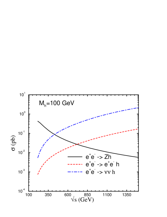
Figure 19: Higgs boson production in $e^{+}e^{-}$ collisions for $M_{h}=100$.

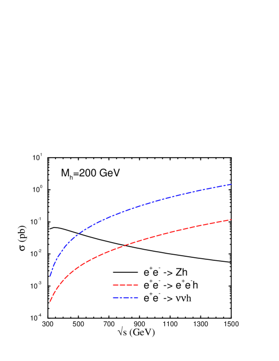
Figure 20: Higgs boson production in $e^{+}e^{-}$ collisions for $M_{h}=200$.

The $ZZ$ fusion cross section, $e^{+}e^{-}\rightarrow e^{+}e^{-}h$, is an order of magnitude smaller than the $W^{+}W^{-}$ fusion process due to the smaller neutral current couplings. This suppression is partially compensated for experimentally by the fact that the $e^{+}e^{-}h$ final state permits a missing mass analysis to determine the Higgs boson mass.

At an $e^{+}e^{-}$ collider with $\sqrt{s}\sim 350~{}GeV$, the cross section for vector boson fusion, $e^{+}e^{-}\rightarrow W^{+}W^{-}\nu{\overline{\nu}}\rightarrow h\nu{\overline{\nu}}$, and that for $e^{+}e^{-}\rightarrow Zh$ are of similar size for a $100~{}GeV$ Higgs boson. The fusion processes grow as $(1/M_{W}^{2})\log(s/M_{h}^{2})$, while the $s-$ channel process, $e^{+}e^{-}\rightarrow Zh$, falls as $1/s$ and so at high enough energy the fusion process will dominate, as can be seen in Figs. 19 and 20.

8.2 $e^{+}e^{-}\rightarrow t{\overline{t}}h$

Higgs boson production in association with a $t{\overline{t}}$ pair is small at an $e^{+}e^{-}$ collider. At $\sqrt{s}=500~{}GeV$, $20~{}fb^{-1}$ of luminosity would produce only $20$ events for $M_{h}=100~{}GeV$. The signature for this final state is spectacular, however, since the final state is predominantly $W^{+}W^{-}b{\overline{b}}b{\overline{b}}$, which has a very small background.

The process $e^{+}e^{-}\rightarrow t{\overline{t}}h$ provides a direct mechanism for measuring the $t{\overline{t}}h$ Yukawa coupling. Since this coupling can be significantly different in a supersymmetric model from that in the Standard Model, the measurement would provide a means of discriminating between models. The $t{\overline{t}}h$ Yukawa coupling also enters into the rates for $gg\rightarrow h$ and $h\rightarrow\gamma\gamma$ as these processes have large contributions from top quark loops. However, in these cases it is possible that there is unknown new physics which also enters into the calculation of the rate and dilutes the interpretation of the signal as the measurement of the $t{\overline{t}}h$ coupling.

The rate for $e^{+}e^{-}\rightarrow b{\overline{b}}h$ in the Standard Model is probably not large enough to be measured due to the smallness of the $b{\overline{b}}h$ Yukawa coupling. In supersymmetric models with large $\tan\beta$, however, the rate can be enhanced.

Figure 21: Feynman diagrams contributing to the lowest order process, $e^{+}e^{-}\rightarrow t{\overline{t}}h$.

The cross section for $e^{+}e^{-}\rightarrow t\bar{t}h$ occurs through the Feynman diagrams of Fig. 21.$\!{}^{{\bf?}}$

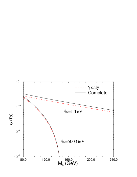
Figure 22: Lowest order cross section for $e^{+}e^{-}\rightarrow t{\overline{t}}h$ at $\sqrt{s}=500$ GeV and $\sqrt{s}=1~{}\mbox{TeV}$. The curve labelled complete includes $\gamma,Z$ exchange, along with bremsstrahlung from the $Z$ boson. We take $M_{t}=175~{}GeV$.

$$\frac{d\sigma(e^{+}e^{-}\rightarrow t\bar{t}h^{0})}{dx_{h}} = N_{c}\frac{\sigma_{0}}{(4\pi)^{2}}\left\{\left[Q_{e}^{2}Q_{t}^{2}+\frac{2Q_{e}Q_{t}V_{e}V_{t}}{1-M_{Z}^{2}/s}\right.\right.$$ (115)

$$\left.+\frac{(V_{e}^{2}+A_{e}^{2})(V_{t}^{2}+A_{t}^{2})}{(1-M_{Z}^{2}/s)^{2}}\right]G_{1}$$

$$+\left.\frac{V_{e}^{2}+A_{e}^{2}}{(1-M_{Z}^{2}/s)^{2}}\left[A_{t}^{2}\sum_{i=2}^{6}G_{i}+V_{t}^{2}(G_{4}+G_{6})\right]\right.$$

$$\left.+\frac{Q_{e}Q_{t}V_{e}V_{t}}{1-M_{Z}^{2}/s}G_{6}\right\}\,\,\,\,,$$

where $\sigma_{0}\!=\!4\pi\alpha^{2}/3s$, $\alpha$ is the QED fine structure constant, $N_{c}=3$ is the number of colors, $x_{h}=2E_{h}/\sqrt{s}$ with $E_{h}$ the Higgs boson energy, and $Q_{i}$, $V_{i}$ and $A_{i}$ ($i\!=\!e$, $t$) denote the electromagnetic and weak couplings of the electron and of the top quark respectively,

$$V_{i}=\frac{2I_{3L}^{i}-4Q_{i}s_{W}^{2}}{4s_{W}c_{W}}\,\,\,\,\,\,\,\,,\,\,\,\,\,\,\ A_{i}=\frac{2I_{3L}^{i}}{4s_{W}c_{W}}\,\,\,\,,$$ (116)

with $I_{3L}^{i}\!=\!\pm 1/2$ being the weak isospin of the left-handed fermions and $s_{W}^{2}\!=\!1-c_{W}^{2}=0.23$.

The coefficients $G_{1}$ and $G_{2}$ describe the radiation of the Higgs boson from the top quark. The other four coefficients, $G_{3},\ldots,G_{6}$ describe the emission of a Higgs boson from the $Z$-boson. Analytic expressions for $G_{i}$ can be found in the first paper of Ref. 62. The most relevant contributions are those in which the Higgs boson is emitted from a top quark leg, i.e. those proportional to $G_{1}$ and $G_{2}$ in Eq. (115). The contribution from the Higgs boson coupling to the $Z$ boson is always less than a few per cent at $\sqrt{s}=500$ GeV and $1$ TeV and can safely be neglected. In Fig. 22, we show the complete cross section for $e^{+}e^{-}\rightarrow t{\overline{t}}h$ production and also the contribution from the photon exchange contribution only. We see that at both $\sqrt{s}=500$ GeV and $1$ TeV, the cross section is well approximated by the photon exchange only.

The ${\cal O}(\alpha_{s})$ corrections to the rate for $e^{+}e^{-}\rightarrow t{\overline{t}}h$ increase the rate significantly at $\sqrt{s}=500$ and are shown in Fig. 23.$\!{}^{{\bf?}}$ The factor $K$ is defined to be the ratio of the ${\cal O}(\alpha_{s})$ corrected rate to the lowest order rate. At $\sqrt{s}=1~{}TeV$, the corrections are small.

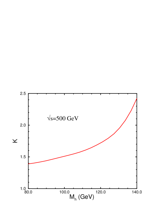
Figure 23: Ratio of the ${\cal O}(\alpha_{s})$ corrected rate to the lowest order cross section for $e^{+}e^{-}\rightarrow t{\overline{t}}h$ at $\sqrt{s}=500$ GeV. We take $M_{t}=175~{}GeV$ and $\alpha_{s}(M_{t}^{2})=.1116$.

Note that the only $\mu$ dependence occurs in $\alpha_{s}(\mu)$. If $\mu=\sqrt{s}$, then $K(M_{h}=100\,\mbox{GeV})$ is reduced to $1.4$ from the value $K=1.5$ obtained with $\mu=M_{t}$ for $\sqrt{s}=500~{}GeV$. Further study is needed of the viability of this process as a means of measuring the $t{\overline{t}}h$ Yukawa coupling.

9 Strongly Interacting Higgs Bosons

We can see from the scalar potential of Eq. 43 that as the Higgs boson grows heavy, its self interactions become large and it becomes strongly interacting. The study of this regime will therefore require new techniques. For $M_{h}>1.4~{}TeV$, the total Higgs boson decay width is larger than its mass and it no longer makes sense to think of the Higgs boson as a particle.$\!{}^{{\bf?}}$ A handy rule of thumb for the heavy Higgs boson is

$$\Gamma(h\rightarrow W^{+}W^{-}+ZZ)\sim 500~{}GeV\biggl{(}{M_{h}\over 1~{}TeV}\biggr{)}^{3}\,\,.$$ (117)

The $TeV$ Higgs boson regime can most easily be studied by going to the Goldstone boson sector of the theory. In Feynman gauge, the three Goldstone bosons, $\omega^{\pm},z$, have mass $M_{\omega,z}=M_{W,Z}$ and have the interactions,

$$V={M_{h}^{2}\over 2v}h\biggl{(}h^{2}+Z^{2}+2\omega^{+}\omega^{-}\biggr{)}+{M_{h}^{2}\over 8v^{2}}\biggl{(}h^{2}+z^{2}+2\omega^{+}\omega^{-}\biggr{)}^{2}.$$ (118)

Calculations involving only the Higgs boson and the Goldstone bosons are easy since the scalar contribution is enhanced by $M_{h}^{2}/v^{2}$, while contributions involving the gauge bosons are proportional to $g^{2}$ and so can be neglected for heavy Higgs bosons. For example the amplitude for $\omega^{+}\omega^{-}\rightarrow\omega^{+}\omega^{-}$ is, $\!{}^{{\bf?}}$

Figure 24: Goldstone boson scattering, $\omega^{+}\omega^{-}\rightarrow\omega^{+}\omega^{-}$.

$${\cal A}(\omega^{+}\omega^{-}\rightarrow\omega^{+}\omega^{-})=-{M_{h}^{2}\over v^{2}}\biggl{(}{s\over s-M_{h}^{2}}+{t\over t-M_{h}^{2}}\biggr{)},$$ (119)

where $s,t,u$ are the Mandelstam variables in the $\omega^{+}\omega^{-}$ center of mass frame. It is instructive to compare Eq. 119 with what is obtained by computing $W^{+}_{L}W^{-}_{L}\rightarrow W^{+}_{L}W^{-}_{L}$ using longitudinally polarized gauge bosons and extracting the leading power of $s$ from each diagram:$\!{}^{{\bf?}}$

$${\cal A}(W^{+}_{L}W^{-}_{L}\rightarrow W^{+}_{L}W^{-}_{L})\sim-{1\over v^{2}}\biggl{\{}-s-t+{s^{2}\over s-M_{h}^{2}}+{t^{2}\over t-M_{h}^{2}}\biggr{\}}\quad.$$ (120)

From Eqs.  119 and  120 we find an amazing result,

$${\cal A}(W^{+}_{L}W^{-}_{L}\rightarrow W^{+}_{L}W^{-}_{L})={\cal A}(\omega^{+}\omega^{-}\rightarrow\omega^{+}\omega^{-})+{\cal O}\biggl{(}{M_{W}^{2}\over s}\biggr{)}.$$ (121)

This result means that instead of doing the complicated calculation with real gauge bosons, we can instead do the easy calculation with only scalars if we are at an energy far above the $W$ mass and are interested only in those effects which are enhanced by $M_{h}^{2}/v^{2}$. This is a general result and has been given the name of the electroweak equivalence theorem.$\!{}^{{\bf?}}$ The electroweak equivalence theorem holds for $S-$ matrix elements; it is not true for individual Feynman diagrams.

The formal statement of the electroweak equivalence theorem is that

$${\cal A}(V_{L}^{1}V_{L}^{2}....V_{L}^{N}\rightarrow V_{L}^{1}V_{L}^{2}....V_{L}^{N^{\prime}}) = (i)^{N}(-i)^{N^{\prime}}{\cal A}(\omega_{1}\omega_{2}...\omega_{N}\rightarrow\omega_{1}\omega_{2}...\omega_{N^{\prime}})$$ (122)

$$~{}~{}+{\cal O}\biggl{(}{M_{V}^{2}\over s}\biggr{)},$$

where $\omega_{i}$ is the Goldstone boson corresponding to the longitudinal gauge boson, $V_{L}^{i}$. In other words, when calculating scattering amplitudes of longitudinal gauge bosons at high energy, we can replace the ${\it external}$ longitudinal gauge bosons by Goldstone bosons. A formal proof of this theorem can be found in Ref. 66.

The electroweak equivalence theorem is extremely useful in a number of applications. For example, to compute the radiative corrections to $h\rightarrow W^{+}W^{-}$ or to $W^{+}_{L}W^{-}_{L}\rightarrow W^{+}_{L}W^{-}_{L}$, the dominant contributions which are enhanced by $M_{h}^{2}/v^{2}$ can be found by computing the one loop corrections to $h\rightarrow\omega^{+}\omega^{-}$ and to $\omega^{+}\omega^{-}\rightarrow\omega^{+}\omega^{-}$ considering only scalar particles.$\!{}^{{\bf?},{\bf?}}$. Probably the most powerful application of the electroweak equivalence theorem is, however, in the search for the physical effects of strongly interacting gauge bosons which we turn to now.

9.1 Unitarity

In the previous section we saw that the Goldstone bosons have interactions which grow with energy. However, models which have cross sections rising with $s$ will eventually violate perturbative unitarity. To see this we consider $2\rightarrow 2$ elastic scattering. The differential cross section is

$${d\sigma\over d\Omega}={1\over 64\pi^{2}s}\mid{\cal A}\mid^{2}.$$ (123)

Using a partial wave decomposition, the amplitude can be written as

$${\cal A}=16\pi\sum_{l=0}^{\infty}(2l+1)P_{l}(\cos\theta)a_{l}\quad,$$ (124)

where $a_{l}$ is the spin $l$ partial wave and $P_{l}(\cos\theta)$ are the Legendre polynomials. The cross section becomes,

$$\sigma = {8\pi\over s}\sum_{l=0}^{\infty}\sum_{l^{\prime}=0}^{\infty}(2l+1)(2l^{\prime}+1)a_{l}a^{*}_{l}$$ (125)

$$\qquad\cdot\int_{-1}^{1}d\cos\theta P_{l}(\cos\theta)P_{l^{\prime}}(\cos\theta)$$

$$= {16\pi\over s}\sum_{l=0}^{\infty}(2l+1)\mid a_{l}\mid^{2}\quad,$$

where we have used the fact that the $P_{l}$’s are orthogonal. The optical theorem gives,

$$\sigma={1\over s}Im\biggl{[}{\cal A}(\theta=0)\biggr{]}={16\pi\over s}\sum_{l=0}^{\infty}(2l+1)\mid a_{l}\mid^{2}.$$ (126)

This immediately yields the unitarity requirement which is illustrated in Fig. 25.

$$\mid a_{l}\mid^{2}=Im(a_{l}).$$ (127)

Figure 25: Argand diagram showing unitarity condition on scattering amplitudes.

From Fig. 25 we see that one statement of unitarity is the requirement that

$$\mid Re(a_{l})\mid<{1\over 2}.$$ (128)

As a demonstration of unitarity restrictions, we consider the scattering of longitudinal gauge bosons, $W^{+}_{L}W^{-}_{L}\rightarrow W^{+}_{L}W^{-}_{L}$, which can be found to ${\cal O}(M_{W}^{2}/s)$ from the Goldstone boson scattering of Fig. 24. We begin by constructing the $J=0$ partial wave, $a_{0}^{0}$, in the limit $M_{W}^{2}<<s$ from Eq. 119,

$$a_{0}^{0}(\omega^{+}\omega^{-}\rightarrow\omega^{+}\omega^{-}) \equiv {1\over 16\pi s}\int^{0}_{-s}\mid{\cal A}\mid dt$$ (129)

$$= -{M_{h}^{2}\over 16\pi v^{2}}\biggl{[}2+{M_{h}^{2}\over s-M_{h}^{2}}-{M_{h}^{2}\over s}\log\biggl{(}1+{s\over M_{h}^{2}}\biggr{)}\biggr{]}.$$

If we go to very high energy, $s>>M_{h}^{2}$, then Eq.  129 has the limit

$$a_{0}^{0}(\omega^{+}\omega^{-}\rightarrow\omega^{+}\omega^{-})\longrightarrow_{s>>M_{h}^{2}}-{M_{h}^{2}\over 8\pi v^{2}}.$$ (130)

Applying the unitarity condition, $\mid Re(a_{0}^{0})\mid<{1\over 2}$ gives the restriction$\!{}^{{\bf?}}$

$$M_{h}<870~{}GeV.$$ (131)

It is important to understand that this does not mean that the Higgs boson cannot be heavier than $870~{}GeV$, it simply means that for heavier masses perturbation theory is not valid. By considering coupled channels, a slightly tighter bound than Eq. 131 can be obtained. The Higgs boson therefore plays a fundamental role in the theory since it cuts off the growth of the partial wave amplitudes and makes the theory obey perturbative unitarity.

We can apply the alternate limit to Eq. 129 and take the Higgs boson much heavier than the energy scale. In this limit$\!{}^{{\bf?}}$

$$a_{0}^{0}(\omega^{+}\omega^{-}\rightarrow\omega^{+}\omega^{-})\longrightarrow_{s<<M_{h}^{2}}-{s\over 32\pi v^{2}}\quad.$$ (132)

Again applying the unitarity condition we find,

$$\sqrt{s_{c}}<1.7~{}TeV\quad.$$ (133)

We have used the notation $s_{c}$ to denote $s$(critical), the scale at which perturbative unitarity is violated. Eq.  133 is the basis for the oft-repeated statement, There must be new physics on the TeV scale. Eq. 133 tells us that without a Higgs boson, there must be new physics which restores perturbative unitarity somewhere below an energy scale of $1.7~{}TeV$.

9.2 $M_{h}\rightarrow\infty$, The Non-Linear Theory

So far we have considered searching for the Higgs boson in various mass regimes. In this section we will consider the consequences of taking the Higgs boson mass much heavier than the energy scale being probed.$\!{}^{{\bf?}}$ In fact, we will take the limit $M_{h}\rightarrow\infty$ and assume that the effective Lagrangian for electroweak symmetry breaking is determined by new physics outside the reach of future accelerators such as the LHC. It is an important question as to whether we can learn something about the nature of the electroweak symmetry breaking in this scenario.

Since we do not know the full theory, we build the effective Lagrangian out of all operators consistent with the unbroken symmetries. In particular, we must include operators of all dimensions, whether or not they are renormalizable. In this way we construct the most general effective Lagrangian that describes electroweak symmetry breaking.

To specify the effective Lagrangian, we must first fix the pattern of symmetry breaking. We will assume that the global symmetry in the scalar sector of the model is $SU(2)_{L}\times SU(2)_{R}$ as in the minimal Standard Model. We will also assume a custodial $SU(2)_{C}$ symmetry.$\!{}^{{\bf?}}$ This is the symmetry which forces $\rho=M_{W}^{2}/(M_{Z}^{2}\cos\theta_{W})=1$. The pattern of global symmetry breaking is then

$$SU(2)_{L}\times SU(2)_{R}\rightarrow SU(2)_{C}.$$ (134)

In this case, the Goldstone bosons can be described in terms of the unitary unimodular field $U$$\!{}^{{\bf?}}$,

$$U\equiv\exp\bigg{(}\frac{i\,\omega_{i}(x)\cdot\tau_{i}}{2v}\bigg{)}\quad.$$ (135)

This is analogous to the Abelian Higgs model where we took the Higgs field to be,

$$\Phi={1\over\sqrt{2}}e^{{i\chi\over v}}(h+v).$$ (136)

Under the global $SU(2)_{L}\times SU(2)_{R}$ symmetry the $U$ field transforms as,

$$U\rightarrow L^{\dagger}UR.$$ (137)

It is straightforward to write down the most general $SU(2)_{L}\times U(1)_{Y}$ gauge invariant Lagrangian which respects the global symmetry of Eq. 134. The Lagrangian can be written in terms of a derivative expansion, where each additional set of derivatives corresponds to an additional power of $s/\Lambda^{2}$, with $\Lambda$ some high scale corresponding to unknown new physics. The lowest order effective Lagrangian (with two derivatives acting on the $U$ field) for the symmetry breaking sector of the theory is then

$${\cal L}_{SM}^{nlr}={v^{2}\over 4}Tr\biggl{[}D_{\mu}U^{\dagger}D^{\mu}U\biggr{]}-{1\over 2}Tr\biggl{(}W^{\mu\nu}W_{\mu\nu}\biggr{)}-{1\over 2}Tr\biggl{(}B_{\mu\nu}B^{\mu\nu}\biggr{)},$$ (138)

where the covariant derivative is given by,

$$D_{\mu}U=\partial_{\mu}U+{i\over 2}gW_{\mu}^{i}\tau^{i}U-{i\over 2}g^{\prime}B_{\mu}U\tau_{3}.$$ (139)

We use the superscript ‘nlr’ to denote ‘nonlinear realization’, since this expansion contains derivative interactions.

The gauge field kinetic energies are matrices in $SU(2)$ space:

$$W_{\mu\nu} \equiv {1\over 2}\biggl{(}\partial_{\nu}W_{\mu}-\partial_{\mu}W_{\nu}-{i\over 2}g[W_{\mu},W_{\nu}]\biggr{)}$$

$$B_{\mu\nu} = {1\over 2}\biggl{(}\partial_{\nu}B_{\mu}-\partial_{\mu}B_{\nu}\biggr{)}\tau_{3}$$ (140)

with $W_{\nu}\equiv W_{\nu}^{i}\cdot\tau_{i}$. In unitary gauge, $U=1$ and it is easy to see that Eq. 138 generates mass terms for the $W$ and $Z$ gauge bosons. The Lagrangian of Eq. 138 is exactly the Standard Model Lagrangian with $M_{h}\rightarrow\infty$. Since no physical Higgs boson is included, ${\cal L}^{nlr}_{SM}$ is non-renormalizable.

Using the Lagrangian of Eq. 138 it is straightforward to compute Goldstone boson scattering amplitudes such as$\!{}^{{\bf?}}$

$${\cal A}(\omega^{+}\omega^{-}\rightarrow zz)={s\over v^{2}}\equiv A(s,t,u)\quad,$$ (141)

which of course agree with those found in the Standard Model when we take $M_{h}^{2}>>s$. Amplitudes which grow with $s$ are a disaster for perturbation theory since eventually they will violate perturbative unitarity as discussed in Sec. 9.2. Of course, this simply tells us that there must be some new physics at high energy.

Because of the custodial $SU(2)_{C}$ symmetry, the various scattering amplitudes are related:

$${\cal A}(\omega^{+}z\rightarrow\omega^{+}z) = A(t,s,u)$$

$${\cal A}(\omega^{+}\omega^{-}\rightarrow\omega^{+}\omega^{-}) = A(s,t,u)+A(t,s,u)$$

$${\cal A}(\omega^{+}\omega^{+}\rightarrow\omega^{+}\omega^{+}) = A(t,s,u)+A(u,t,s)$$

$${\cal A}(zz\rightarrow zz) = A(s,t,u)+A(t,s,u)+A(u,s,t).$$ (142)

The relationships of Eq. 142 were discovered by Weinberg$\!{}^{{\bf?}}$ over 30 years ago for the case of $\pi\pi$ scattering, which has the same global $SU)2)_{L}\times SU(2)_{R}$ global symmetry.

Using the electroweak equivalence theorem, the Goldstone boson scattering amplitudes can be related to the amplitudes for longitudinal gauge boson scattering. The effective $W$ approximation can then be used to find the physical scattering cross sections for hadronic and $e^{+}e^{-}$ interactions in the scenario where there is an infinitely massive (or no) Higgs boson.

Eq.  138 is a non-renormalizable effective Lagrangian which must be interpreted as an expansion in powers of $s/\Lambda^{2}$, where $\Lambda$ can be taken to be the scale of new physics which restores unitarity (say $M_{h}$ in a theory with a Higgs boson). The effective Lagrangian can be written as,

$${\cal L}_{\rm eff}^{\rm nlr}={\cal L}_{\rm SM}^{\rm nlr}+\sum_{i}\alpha_{i}{\cal O}_{i}+\cdots\;.$$ (143)

To ${\cal O}(s^{2})$ we have the non-Standard Model operators with four or fewer derivatives which conserve CP and preserve the custodial $SU(2)_{C}$ symmetry, $\!{}^{{\bf?}}$

$${\cal L}_{1} = \frac{1}{2}\alpha_{1}gg^{\prime}Tr\biggl{(}B_{\mu\nu}TW^{\mu\nu}\biggr{)}\;,$$

$${\cal L}_{2} = \frac{i}{2}\alpha_{2}g^{\prime}B_{\mu\nu}Tr\biggl{(}T[V^{\mu},V^{\nu}]\biggr{)}\;,$$

$${\cal L}_{3} = i\alpha_{3}gTr\biggl{(}W_{\mu\nu}[V^{\mu},V^{\nu}]\biggr{)}\;,$$

$${\cal L}_{4} = \alpha_{4}\biggl{[}Tr(V_{\mu}V_{\nu})\biggr{]}^{2}\;,$$

$${\cal L}_{5} = \alpha_{5}\biggl{[}Tr(V_{\mu}V^{\mu})\biggr{]}^{2}\;,$$ (144)

where

$$T \equiv 2UT^{3}U^{\dagger}\;,$$

$$V_{\mu} \equiv (D_{\mu}U)U^{\dagger}\;,$$ (145)

and $T_{i}=\tau_{i}/2$ with the normalization Tr$(T_{i}T_{j})=\frac{1}{2}\delta_{ij}$. This is the most general $SU(2)_{L}\times U(1)_{Y}$ gauge invariant set of interactions of ${\cal O}(s^{2})$ which preserves the custodial $SU(2)_{C}$. The coefficients, $\alpha_{i}$, have information about the underlying dynamics of the theory. By measuring the various coefficients one might hope to learn something about the mechanism of electroweak symmetry breaking even if the energy of an experiment is below the scale at which the new physics occurs.

If the assumption that there is a custodial $SU(2)_{C}$ is relaxed then there is an additional term with two derivatives and six additional terms with four derivatives,

$${\cal L}_{1}^{\prime} = {\beta_{1}\over 4}v^{2}\biggl{[}Tr(TV_{\mu})\biggr{]}^{2}\;,$$

$${\cal L}_{6} = \alpha_{6}Tr\biggl{(}V_{\mu}V_{\nu}\biggr{)}Tr\biggl{(}TV^{\mu}\biggr{)}Tr\biggl{(}TV^{\nu}\biggr{)}\;,$$

$${\cal L}_{7} = \alpha_{7}Tr\biggl{(}V_{\mu}V^{\mu}\biggr{)}Tr\biggl{(}TV_{\nu}\biggr{)}Tr\biggl{(}TV^{\nu}\biggr{)}\;,$$

$${\cal L}_{8} = \frac{1}{4}\alpha_{8}g^{2}\biggl{[}Tr(TW_{\mu\nu})\biggr{]}^{2}\;,$$

$${\cal L}_{9} = \frac{i}{2}\alpha_{9}gTr\biggl{(}TW_{\mu\nu}\biggr{)}Tr\biggl{(}T[V^{\mu},V^{\nu}]\biggr{)}\;,$$

$${\cal L}_{10} = \frac{1}{2}\alpha_{10}\biggl{[}Tr(TV_{\mu})Tr(TV_{\nu})\biggr{]}^{2}\;,$$

$${\cal L}_{11} = \alpha_{11}g\,\epsilon^{\mu\nu\rho\sigma}Tr\biggl{(}TV_{\mu}\biggr{)}Tr\biggl{(}V_{\nu}W_{\rho\sigma}\biggr{)}\;.$$ (146)

The first term ${\cal L}^{\prime}$ corresponds to a non-Standard Model contribution to the $\rho$ parameter.

Since the theory contains no Higgs boson, it is non-renormalizable and so loop corrections will generate singularities. At each order in the energy expansion new effective operators arise whose effects will cancel the singularities generated by loops computed using the Lagrangian corresponding to the order below in $s/\Lambda^{2}$. To ${\cal O}(s^{2})$, the infinities which arise at one loop can all be absorbed by defining renormalized parameters, $\alpha_{i}(\mu)$. The coefficients thus depend on the renormalization scale $\mu$.

As an example, we calculate the loop corrections to the gauge boson two point functions from the new operators of Eqs. 144 and 146.$\!{}^{{\bf?}}$ We compute only the divergent contributions and make the identification

$${1\over\epsilon}(4\pi)^{\epsilon}\Gamma(1+\epsilon)\rightarrow\log\biggl{(}{\Lambda^{2}\over\mu^{2}}\biggr{)}$$ (147)

and drop all nonlogarithmic terms. Furthermore, we chose $\mu^{2}=M_{Z}^{2}$. This gives an estimate of the size of the new physics corrections.

The contributions of the two point functions to four fermion amplitudes is generally summarized by a set of parameters such as the $S$, $T$ and $U$ parameters of Ref. 75. Three of the operators, ${\cal L}_{1}^{\prime}$, ${\cal L}_{1}$ and ${\cal L}_{8}$, contribute at the tree-level to the gauge-boson two-point-functions. Both ${\cal L}_{1}^{\prime}$ and ${\cal L}_{8}$ violate the custodial $SU(2)_{C}$ symmetry and so are expected to be small. The two point functions arising from the Lagrangian of Eqs. 144 and 146 give contributions to $S$, $T$, and $U$ to one-loop, $\!{}^{{\bf?}}$

$$\alpha\Delta S = \frac{\alpha}{12\pi}\log\biggl{(}{\Lambda^{2}\over M_{h}^{2}}\biggr{)}-4e^{2}\alpha_{1}$$

$$\mbox{}-\frac{g^{2}e^{2}}{16\pi^{2}}\biggl{[}{1+30c_{W}^{2}\over 3c_{W}^{2}}+\frac{1-22c_{W}^{2}}{3c_{W}^{2}}\alpha_{3}+\frac{1+6c_{W}^{2}}{3c_{W}^{2}}\alpha_{9}\bigg{]}\log\bigg{(}\frac{\Lambda^{2}}{m_{Z}^{2}}\bigg{)}\;,$$

$$\alpha\Delta T = \frac{3\alpha}{16\pi c_{W}^{2}}\log\biggl{(}{\Lambda^{2}\over M_{h}^{2}}\biggr{)}+2\beta_{1}-\frac{g^{4}}{16\pi^{2}c_{W}^{2}}\bigg{[}\frac{3s_{W}^{2}(3c_{W}^{2}-1)}{2c_{W}^{2}}\alpha_{2}$$

$$+3s_{W}^{2}\alpha_{3}+\frac{15s_{W}^{2}(c_{W}^{2}+1)}{4c_{W}^{2}}\alpha_{4}+\frac{3s_{W}^{2}(c_{W}^{2}+1)}{2c_{W}^{2}}\alpha_{5}$$

$$\mbox{}+\frac{3(2c_{W}^{4}+11)}{4c_{W}^{2}}\alpha_{6}+\frac{6(c_{W}^{4}+1)}{c_{W}^{2}}\alpha_{7}+\frac{3s_{W}^{2}}{2}\alpha_{9}+\frac{9}{c_{W}^{2}}\alpha_{10}\bigg{]}\log\bigg{(}\frac{\Lambda^{2}}{m_{Z}^{2}}\bigg{)}\;,$$

$$\alpha\Delta U = -4e^{2}\alpha_{8}+\frac{g^{4}}{16\pi^{2}}\frac{2s_{W}^{2}}{3c_{W}^{2}}\bigg{[}-s_{W}^{2}(2c_{W}^{2}+3)\alpha_{2}$$ (148)

$$\mbox{}+2s_{W}^{2}(2s_{W}^{2}+c_{W}^{2})\alpha_{3}+(2c_{W}^{4}-15c_{W}^{2}+1)\alpha_{9}\bigg{]}\log\bigg{(}\frac{\Lambda^{2}}{m_{Z}^{2}}\bigg{)}\;,$$

where $s_{W}^{2}=\sin^{2}\theta_{W}=.23$ and $c_{W}^{2}=\cos\theta_{W}^{2}$. Even when all the $\alpha_{i}$ are zero, the expressions for $\Delta S$ and $\Delta T$ are nonzero. This is because the nonlinear Lagrangian contains singularities which in the Standard Model would be cancelled by the contributions of the Higgs boson. In these terms the renormalization scale, ${\hat{\mu}}$, is appropriately taken to be the same Higgs-boson mass we use to evaluate the Standard Model contributions.

Due to the extraordinary precision of electroweak data at low energy and on the $Z$ pole, it is possible to place constraints on models for physics beyond the Standard Model by studying these loop-level contributions of new physics to electroweak observables.$\!{}^{{\bf?}}$ First we analyze the numerical constraints on $\alpha_{1}$, $\beta_{1}$ and $\alpha_{8}$ (which arise from $\Delta S$, $\Delta T$ and $\Delta U$, respectively), and we present the best-fit central values with one-sigma errors,

$$\left.\begin{array}[]{lll}\alpha_{1}&=&(4.7\pm 2.6)\times 10^{-3}\;,\\ \beta_{1}&=&(0.30\pm 0.57)\times 10^{-3}\;,\\ \alpha_{8}&=&(-0.9\pm 7.6)\times 10^{-3}\;.\end{array}\right.$$ (149)

We use $\Lambda=2$ TeV everywhere in this section. These constraints are sufficiently strong that there is no sensitivity to these three parameters at LEP 2.$\!{}^{{\bf?}}$ Observe that a positive value for $\alpha_{1}$ is favored.

Two of the operators, ${\cal L}_{1}$ and ${\cal L}_{8}$, contribute at the tree-level to the gauge-boson two-point-functions and also to nonstandard $WW\gamma$ and $WWZ$ couplings. These are sufficiently constrained by the limits on the two-point functions that we will not consider their contributions to the three point functions. Three operators, ${\cal L}_{2}$, ${\cal L}_{3}$ and ${\cal L}_{9}$, contribute to $WW\gamma$ and $WWZ$ couplings without making a tree-level contribution to the gauge-boson propagators. Much of the literature describes nonstandard $WW\gamma$ and $WWZ$ vertices via the phenomenological effective Lagrangian$\!{}^{{\bf?}}$,

$${\cal L}_{WWV}=$$ (150)

$$-ig_{WWV}\Bigg{\{}g_{1}^{V}\Big{(}{\tilde{W}}^{+}_{\mu\nu}W^{-\,\mu}V^{\nu}-W^{+}_{\mu}V_{\nu}{\tilde{W}}^{-\,\mu\nu}\Big{)}$$

$$+\kappa_{V}W_{\mu}^{+}W_{\nu}^{-}{\tilde{V}}^{\mu\nu}+\frac{\lambda_{V}}{m_{W}^{2}}{\tilde{W}}^{+}_{\mu\nu}{\tilde{W}}^{-\,\nu\rho}{\tilde{V}}_{\rho}^{\;\mu}\Bigg{\}}\;,$$

where $V=Z,\gamma$, the overall coupling constants are $g_{WW\gamma}=e$ and $g_{WWZ}=g\cos\theta_{W}$. The field-strength tensors include only the Abelian parts, i.e. ${\tilde{W}}^{\mu\nu}=\partial^{\mu}W^{\nu}-\partial^{\nu}W^{\mu}$ and ${\tilde{V}}^{\mu\nu}=\partial^{\mu}V^{\nu}-\partial^{\nu}V^{\mu}$. The coefficients of the electroweak chiral Lagrangian to ${\cal O}(s^{2})$ in the energy expansion can be matched to the parameterization of Eq. 150, demonstrating that the two approaches are equivalent: $\!{}^{{\bf?},{\bf?}}$

$$g_{1}^{Z}(q^{2}) = 1+{g^{2}\over\cos\theta_{W}^{2}}\alpha_{3}\;,$$ (151)

$$\kappa_{\gamma}(q^{2}) = 1+g^{2}\Big{(}\alpha_{2}+\alpha_{3}+\alpha_{9}\Big{)}\;,$$ (152)

$$\kappa_{Z}(q^{2}) = 1+{g^{2}\over\cos^{2}\theta_{W}}\Big{(}-\sin^{2}\theta_{W}\alpha_{2}+\cos^{2}\theta_{W}(\alpha_{3}+\alpha_{9})\Big{)}\;,$$ (153)

$$\lambda_{\gamma}(q^{2}) = \lambda_{Z}(q^{2})\approx 0\;.$$ (154)

If we impose the custodial SU(2)_C symmetry on the new physics, then we may neglect the $\alpha_{9}$ terms. Eqn. (154) reflects our prejudice that the $\lambda_{V}$ couplings, being generated by ${\cal O}(s^{3})$ operators while the other couplings are generated by ${\cal O}(s^{2})$ operators, should be relatively small.

We place constraints on the operators contributing to the 3-point function by considering the effects of only one operators at a time.

Table 2: $95\%$ confidence level constraints for $\Lambda=2~{}TeV$. In the first row, all other coefficients are set to zero. In the second row, $\alpha_{1}=5.5\times 10^{-3}$ is chosen according to Eq. 154. $\alpha_{2}$ $\alpha_{3}$ $\alpha_{9}$ $\alpha_{1}=0$ 0.21$\pm$0.15 -0.17$\pm$0.11 0.16$\pm$0.67 $\alpha_{1}=5.5\times 10^{-3}$ 0.05$\pm$0.15 -0.04$\pm$0.11 -0.02$\pm$0.67

Note that in the first row of Table 2, when $\alpha_{1}=0$, only $\alpha_{9}$ is consistent with the Standard Model at the 95% confidence level. However, in the second row where we have chosen the central value of $\alpha_{1}$ according to the best-fit value of Eqn. (149), all of the central values are easily consistent with the Standard Model. While the central values easily move around as we include additional operators in the analysis, the errors are much more robust.

The effects of the non-Standard Model gauge boson couplings can also be searched for in $e^{+}e^{-}$ and hadron machines which are sensitive to both the three and four gauge boson vertices through vector boson scattering.$\!{}^{{\bf?},{\bf?}}$ Since the effects grow with energy, the LHC will be much more sensitive than the Tevatron to non-Standard Model gauge boson couplings. To study strong interactions with the Lagrangian of Eqs.  144 and 146, the effective $W$ approximation can be used to get results for hadronic interactions or $e^{+}e^{-}$ scattering.

9.3 Coefficients of New Interactions in a Strongly Interacting Symmetry Breaking Sector

It is instructive to estimate the size of the $\alpha_{i}$ coefficients in typical theories. Using the effective Lagrangian approach this can be done in a consistent way. In any realistic scenario there will be a set of nonzero $\alpha_{i}$, and it is possible (indeed likely) that there will be large interferences between the effects of the various coefficients. In order to see the types of limits which might arise in various scenarios of spontaneous symmetry breaking, we consider a strongly interacting scalar in order to obtain an indication of the sensitivity of our results to the underlying dynamics. Using the effective-Lagrangian approach, we can estimate the coefficients in a consistent way.

We first consider a model with three Goldstone bosons corresponding to the longitudinal components of the $W^{\pm}$ and $Z$ bosons coupled to a scalar isoscalar resonance like the Higgs boson. We assume that the $\alpha_{i}(\mu^{2})$ are dominated by tree-level exchange of the scalar boson. Integrating out the scalar and matching the coefficients at the scale $M_{h}$ gives the predictions, $\!{}^{{\bf?}}$

$$\alpha_{4}(\mu^{2}) = \frac{1}{16\pi^{2}}\frac{1}{12}\log\bigg{(}\frac{m_{H}^{2}}{\mu^{2}}\bigg{)}$$ (155)

$$= 2\alpha_{2}(\mu^{2})=2\alpha_{3}(\mu^{2})=-\alpha_{1}(\mu^{2})$$ (156)

$$\alpha_{5}(\mu^{2}) = \frac{1}{16\pi^{2}}\Bigg{[}\frac{1}{24}\log\bigg{(}\frac{m_{H}^{2}}{\mu^{2}}\bigg{)}+\frac{64\pi^{3}}{3}\frac{\Gamma_{h}v^{4}}{m_{H}^{5}}\Bigg{]},$$ (157)

where $\Gamma_{h}$ is the width of the scalar into Goldstone bosons. All of the other $\alpha_{i}$ are zero in this scenario. It is important to note that only the logarithmic terms are uniquely specified. The constant terms depend on the renormalization scheme.

In Fig. 26

Figure 26: 95% confidence level contours for $\Lambda=$ 2 TeV and $M_{t}=$ 175 GeV for two values of $\mu$ in a model with a strongly interacting scalar, (cf Eqs. 160-162 ).

we plot $\alpha_{5}(\mu^{2})$ vs. $\alpha_{1}(\mu^{2})$ with the pattern typical of a theory dominated by a heavy scalar given in Eqn. 157, $-\alpha_{1}(\mu^{2})=2\alpha_{2}(\mu^{2})=2\alpha_{3}(\mu^{2})=\alpha_{4}(\mu^{2})$. First of all, notice that the contour obtained depends rather strongly upon our choice of the renormalization scale, $\mu$, especially with regard to the $\alpha_{5}$ axis. Everything to the right of $\alpha_{1}=0$ corresponds to $m_{H}<\mu$. Furthermore, since we require that $\Gamma_{h}$ be non-negative, we may approximately exclude everything below the $\alpha_{5}=0$ axis. The allowed region to the upper right of the figure corresponds to a Higgs-boson with a mass in the MeV range and an extremely narrow width; this portion of the figure is already excluded by experiment. The positive central value of $\alpha_{1}$ indicates that a heavy scalar resonance is disfavored, in agreement with the indirect limits from LEP2 discussed in Section 3.3.

10 Problems with the Higgs Mechanism

In the preceeding sections we have discussed many features of the Higgs mechanism. However, most theorists firmly believe that the Higgs mechanism cannot be the entire story behind electroweak symmetry breaking. The primary reasons are:

• The Higgs sector of the theory is trivial ($\lambda\rightarrow 0$ as the energy scale $\rightarrow\infty$) unless the Higgs mass is in a very restricted range.

• The Higgs mechanism doesn’t explain why $v=246~{}GeV$.

• The Higgs mechanism doesn’t explain why fermions have the masses they do.

• Loop corrections involving the Higgs boson are quadratically divergent and counterterms must be adjusted order by order in perturbation theory to cancel these divergences. This fine tuning is considered by most theorists to be unnatural.

10.1 Quadratic Divergences

The most compelling argument against the simplest version of the Standard Model is the quadratically divergent contributions to the Higgs boson mass which arise when loop corrections are computed. At one loop, the quartic self- interactions of the Higgs boson generate a quadratically divergent contribution to the Higgs boson mass which must be cancelled by a mass counterterm. This counterterm must be fine tuned at each order in perturbation theory. We begin by considering a theory with a single fermion, $\psi$, coupled to a massive Higgs scalar,

$${\cal L}_{\phi}={\overline{\psi}}(i\partial)\psi+\mid\partial_{\mu}\phi\mid^{2}-m_{S}^{2}\mid\phi\mid^{2}-\biggl{(}\lambda_{F}{\overline{\psi}}\psi\phi+{\rm h.c.}\biggr{)}\quad.$$ (158)

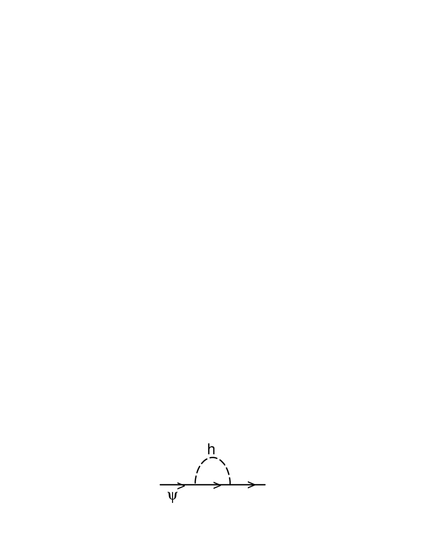
Figure 27: Scalar contribution to fermion mass renormalization.

We will assume that this Lagrangian leads to spontaneous symmetry breaking and so take $\phi=(h+v)/\sqrt{2}$, with $h$ the physical Higgs boson. After spontaneous symmetry breaking, the fermion acquires a mass, $m_{F}=\lambda_{F}v/\sqrt{2}$. First, let us consider the fermion self-energy arising from the scalar loop corresponding to Fig. 27.

$$-i\Sigma_{F}(p)=\biggl{(}{-i\lambda_{F}\over\sqrt{2}}\biggr{)}^{2}(i)^{2}\int{d^{4}k\over(2\pi)^{4}}{(k+m_{F})\over[k^{2}-m_{F}^{2}][(k-p)^{2}-m_{S}^{2}]}\quad.$$ (159)

The renormalized fermion mass is $m_{F}^{r}=m_{F}+\delta m_{F}$, with

$$\delta m_{F} = \Sigma_{F}(p)\mid_{p=m_{F}}$$ (160)

$$= i{\lambda_{F}^{2}\over 32\pi^{4}}\int_{0}^{1}dx\int d^{4}k^{\prime}{m_{F}(1+x)\over[k^{\prime 2}-m_{F}^{2}x^{2}-m_{S}^{2}(1-x)]^{2}}\quad.$$

The integral can be performed in Euclidean space, which amounts to making the following transformations,

$$k_{0} \rightarrow ik_{4}$$

$$d^{4}k^{\prime} \rightarrow id^{4}k_{E}$$

$$k^{\prime 2} \rightarrow -k_{E}^{2}\quad.$$ (161)

Since the integral of Eq. 160 depends only on $k_{E}^{2}$, it can easily be performed using the result (valid for symmetric integrands),

$$\int d^{4}k_{E}f(k_{E}^{2})=\pi^{2}\int^{\Lambda^{2}}_{0}ydyf(y)\quad.$$ (162)

In Eq. 162, $\Lambda$ is a high energy cut-off, presumably of the order of the Planck scale or a grand unified scale. The renormalization of the fermion mass is then,

$$\delta m_{F} = -{\lambda_{F}^{2}m_{F}\over 32\pi^{2}}\int_{0}^{1}~{}dx(1+x)\int^{\Lambda^{2}}_{0}{ydy\over[y+m_{F}^{2}x^{2}+m_{S}^{2}(1-x)]^{2}}$$ (163)

$$= -{3\lambda_{F}^{2}m_{F}\over 64\pi^{2}}\log\biggl{(}{\Lambda^{2}\over m_{F}^{2}}\biggr{)}+....$$

where the $....$ indicates terms independent of the cutoff or which vanish when $\Lambda\rightarrow\infty$. This correction clearly corresponds to a well-defined expansion for $m_{F}$. The corrections to fermion masses are said to be natural. In the limit in which the fermion mass vanishes, Eq. 158 is invariant under the chiral transformations,

$$\psi_{L} \rightarrow e^{i\theta_{L}}\psi_{L}$$

$$\psi_{R} \rightarrow e^{i\theta_{R}}\psi_{R},$$ (164)

and so setting the fermion mass to zero increases the symmetry of the theory. Since the Yukawa coupling (proportional to the mass term) breaks this symmetry, the corrections to the mass must be proportional to $m_{F}$.

The situation is quite different, however, when we consider the renormalization of the scalar mass from a fermion loop (Fig. 28) using the same Lagrangian (Eq. 158),

Figure 28: Fermion contribution to the renormalization of a scalar mass.

$$-i\Sigma_{S}(p^{2})=\biggl{(}{-i\lambda_{F}\over\sqrt{2}}\biggr{)}(i)^{2}(-1)\int{d^{4}k\over(2\pi)^{4}}{Tr[(k+m_{F})((k-p)+m_{F})]\over(k^{2}-m_{F}^{2})[(k-p)^{2}-m_{F}^{2}]}\quad.$$ (165)

The minus sign is the consequence of Fermi statistics and will be quite important later. Integrating with a momentum space cutoff as above we find the contribution to the Higgs mass,

$$(\delta M_{h}^{2})_{a}\equiv\Sigma_{S}(m_{S}^{2}) = -{\lambda_{F}^{2}\over 8\pi^{2}}\biggl{[}\Lambda^{2}+(m_{S}^{2}-6m_{F}^{2})\log\biggl{(}{\Lambda\over m_{F}}\biggr{)}$$ (166)

$$~{}~{}+(2m_{F}^{2}-{m_{S}^{2}\over 2})\biggl{(}1+I_{1}\biggl{(}{m_{S}^{2}\over m_{F}^{2}}\biggr{)}\biggr{)}\biggr{]}~{}$$

$$~{}~{}+{\cal O}\biggl{(}{1\over\Lambda^{2}}\biggr{)},$$

where $I_{1}(a)\equiv\int^{1}_{0}dx\log(1-ax(1-x))$. The Higgs boson mass diverges quadratically! The Higgs boson thus does not obey the decoupling theorem$\!{}^{{\bf?}}$ and this quadratic divergence appears independent of the mass of the Higgs boson. Note that the correction is not proportional to $M_{h}$. This is because setting the Higgs mass equal to zero does not increase the symmetry of the Lagrangian. There is nothing that protects the Higgs mass from these large corrections and, in fact, the Higgs mass wants to be close to the largest mass scale in the theory.

Since we know that the physical Higgs boson mass, $M_{h}$, must be less than around $1~{}TeV$ (in order to keep the $WW$ scattering cross section from violating unitarity), we have the unpleasant result,

$$M_{h}^{2}=M_{h,0}^{2}+\delta M_{h}^{2}+{\hbox{counterterm}},$$ (167)

where the counterterm must be adjusted to a precision of roughly $1$ part in $10^{15}$ in order to cancel the quadratically divergent contributions to $\delta M_{h}$. This is known as the “hierarchy problem”. Of course, the quadratic divergence can be renormalized away in exactly the same manner as for logarithmic divergences by adjusting the cut-off. There is nothing formally wrong with this fine tuning. Most theorists, however, regard this solution as unattractive.

The effects of scalar particles on the Higgs mass renormalization are quite different from those of fermions. We introduce two complex scalar fields, $\phi_{1}$ and $\phi_{2}$, interacting with the Standard Model Higgs boson, $h$, (the reason for introducing $2$ scalars is that with foresight we know that a supersymmetric theory associates $2$ complex scalars with each massive fermion – we could just as easily make the argument given below with one additional scalar and slightly different couplings),

$${\cal L} = \mid\partial_{\mu}\phi_{1}\mid^{2}+\mid\partial_{\mu}\phi_{2}\mid^{2}-m_{s_{1}}^{2}\mid\phi_{1}\mid^{2}-m_{s_{2}}^{2}\mid\phi_{2}\mid^{2}$$ (168)

$$~{}~{}+\lambda_{S}\phi\biggr{(}\mid\phi_{1}\mid^{2}+\mid\phi_{1}\mid^{2}\biggr{)}+{\cal L}_{\phi}\quad.$$

Figure 29: Scalar contributions to Higgs mass renormalization.

From the diagrams of Fig. 29, we find the contribution to the Higgs mass renormalization,

$$(\delta M_{h}^{2})_{b} = -\lambda_{S}\int{d^{4}k\over(2\pi)^{4}}\biggl{[}{i\over k^{2}-m_{s_{1}}^{2}}+{i\over k^{2}-m_{s_{2}}^{2}}\biggr{]}$$ (169)

$$= {\lambda_{S}\over 16\pi^{2}}\biggl{\{}2\Lambda^{2}-2m_{s_{1}}^{2}\log\biggl{(}{\Lambda\over m_{s_{1}}}\biggr{)}-2m_{s_{2}}^{2}\log\biggl{(}{\Lambda\over m_{s_{2}}}\biggr{)}\biggr{\}}$$

$$~{}~{}+{\cal O}\biggl{(}{1\over\Lambda^{2}}\biggr{)}.$$

From Eqs. 166 and 169, we see that if

$$\lambda_{S}=\lambda_{F}^{2},$$ (170)

the quadratic divergences coming from these two terms exactly cancel each other. Notice that the cancellation occurs independent of the masses, $m_{F}$ and $m_{s_{i}}$, and of the magnitude of the couplings $\lambda_{S}$ and $\lambda_{F}$.

In the Standard Model, one could attempt to cancel the quadratic divergences in the Higgs boson mass by balancing the contribution from the Standard Model Higgs quartic coupling with that from the top quark loop in exactly the same manner as above. This approach gives a prediction for the Higgs boson mass in terms of the top quark mass. However, since there is no symmetry to enforce this relationship, this cancellation of quadratic divergences fails at $2-$ loops.

Figure 30: Scalar contributions to Higgs mass renormalization.

After the spontaneous symmetry breaking, Eq. 168 also leads to a cubic interaction shown in Fig. 30. These graphs also give a contribution to the Higgs mass renormalization, although they are not quadratically divergent.

$$(\delta M_{h}^{2})_{c} = {\lambda_{S}^{2}v^{2}\over 16\pi^{2}}\biggl{\{}-1+2\log\biggl{(}{\Lambda\over m_{s_{1}}}\biggr{)}-I_{1}\biggl{(}{M_{h}^{2}\over m_{s_{1}}^{2}}\biggr{)}\biggr{\}}+(m_{s_{1}}\rightarrow m_{s_{2}})$$ (171)

$$~{}~{}+{\cal O}\biggl{(}{1\over\Lambda^{2}}\biggr{)}.$$

Combining the three contributions to the Higgs mass and assuming $\Lambda_{S}=\Lambda_{F}^{2}$ and $m_{s_{1}}=m_{s_{1}}$ we find no quadratic divergences,

$$(\delta M_{h}^{2})_{tot}={\lambda_{F}^{2}\over 4\pi^{2}}\biggl{\{}m_{s_{1}}^{2}\log\biggl{(}{\Lambda\over m_{s_{1}}}\biggr{)}-m_{F}^{2}\log\biggl{(}{\Lambda\over m_{F}}\biggr{)}\biggr{\}}+{\cal O}\biggl{(}{1\over\Lambda^{2}}\biggr{)}.$$ (172)

If the mass splitting between the fermion and scalar is small, $\delta m^{2}\equiv m_{F}^{2}-m_{s_{1}}^{2}$, then we have the approximate result,

$$(\delta M_{h}^{2})_{tot}\sim{\lambda_{F}^{2}\over 8\pi^{2}}\delta m^{2}\quad.$$ (173)

Therefore, as long as the mass splitting between scalars and fermions is “small”, no unnatural cancellations will be required and the theory can be considered “natural”.

One alternative to the Standard Model Higgs mechanism is that the Standard Model becomes supersymmetric. In these theories, there is a scalar associated with each fermion and the couplings are just those of Eq. 170. The electroweak symmetry is still broken by the Higgs mechanism, but the quadratic divergences in the scalar sector are cancelled automatically because of the expanded spectrum of the theory and so the model is no longer considered to be unnatural. In the next section, we will briefly discuss the phenomenology of the Higgs bosons occurring in supersymmetric models and emphasize the similarity of much of the phenomenology to that of the Standard Model Higgs.$\!{}^{{\bf?},{\bf?}}$

11 Higgs Bosons in Supersymmetric Models

Supersymmetry is a symmetry which relates particles of differing spin, (in the above example, fermions and scalars). The particles are combined into ${\it superfields}$, which contain fields differing by one-half unit of spin.$\!{}^{{\bf?}}$ The simplest example, the scalar superfield, contains a complex scalar, $S$, and a two- component Majorana fermion, $\psi$. The supersymmetry then completely specifies the allowed interactions.

In a supersymmetric theory the scalars and fermions in a superfield have the same couplings to gauge bosons and so the cancellation of quadratic divergences occurs automatically as in the previous section. This is one of the primary motivations for introducing supersymmetric models. The supersymmetric Lagrangian contains scalar and fermion pairs ${\it of~{}equal~{}mass}$ and so the supersymmetry connects particles of different spin, but with all other characteristics the same. It is clear, then, that supersymmetry must be a broken symmetry. There is no scalar particle, for example, with the mass and quantum numbers of the electron. In fact, there are no candidate supersymmetric scalar partners for any of the fermions in the experimentally observed spectrum. We will take a non-zero mass splitting between the particles of a superfield as a signal for supersymmetry breaking.

Supersymmetric theories are easily constructed according to the rules of supersymmetry. There are two types of superfields relevant for our purposes:

1. ${\it Chiral~{}Superfields}$: These consist of a complex scalar field, $S$, and a $2$-component Majorana fermion field, ${\psi}$.

2. ${\it MasslessVector~{}Superfields}$: These consist of a massless gauge field with field strength $F_{\mu\nu}^{A}$ and a $2$-component Majorana fermion field, $\lambda_{A}$, termed a ${\it gaugino}$. The index $A$ is the gauge index.

The minimal supersymmetric model (MSSM) respects the same $SU(3)\times SU(2)_{L}\times U(1)_{Y}$ gauge symmetries as does the Standard Model. The particles necessary to construct the minimal supersymmetric version of the Standard Model are shown in Tables 3 and 4 in terms of the superfields, (which are denoted by the superscript “hat”). Since there are no candidates for supersymmetric partners of the observed particles, we must double the entire spectrum, placing the observed particles in superfields with new postulated superpartners. There are, of course, quark and lepton superfields for all $3$ generations and we have listed in Table 3 only the members of the first generation. The superfield ${\hat{Q}}$ thus consists of an $SU(2)_{L}$ doublet of quarks:

$$Q_{L}=\left(\begin{array}[]{c}u\\ d\end{array}\right)_{L}$$ (174)

and their scalar partners which are also in an $SU(2)_{L}$ doublet,

$${\tilde{Q}}_{L}=\left(\begin{array}[]{c}{\tilde{u}}_{L}\\ {\tilde{d}}_{L}\end{array}\right)\quad.$$ (175)

Similarly, the superfield ${\hat{U}}^{c}$ (${\hat{D}}^{c}$) contains the right-handed up (down) anti-quark, ${\overline{u}}_{R}$ (${\overline{d}}_{R}$), and its scalar partner, ${\tilde{u}}_{R}^{*}$ (${\tilde{d}}_{R}^{*}$). The scalar partners of the quarks are fancifully called squarks. We see that each quark has $2$ scalar partners, one corresponding to each quark chirality. The leptons are contained in the $SU(2)_{L}$ doublet superfield ${\hat{L}}$ which contains the left-handed fermions,

$$L_{L}=\left(\begin{array}[]{c}\nu\\ e\end{array}\right)_{L}$$ (176)

and their scalar partners,

$${\tilde{L}}_{L}=\left(\begin{array}[]{c}{\tilde{\nu}}_{L}\\ {\tilde{e}}_{L}\end{array}\right)\quad.$$ (177)

Finally, the right-handed anti-electron, ${\overline{e}}_{R}$, is contained in the superfield ${\hat{E}}^{c}$ and has a scalar partner ${\tilde{e}}_{R}^{*}$. The scalar partners of the leptons are termed sleptons.

The $SU(3)\times SU(2)_{L}\times U(1)$ gauge fields all obtain Majorana fermion partners in a supersymmetric model. The ${\hat{G}}^{a}$ superfield contains the gluons, $g^{a}$, and their partners the gluinos, ${\tilde{g}}^{a}$; ${\hat{W}}_{i}$ contains the $SU(2)_{L}$ gauge bosons, $W_{i}$ and their fermion partners, ${\tilde{\omega}}_{i}$ (winos); and ${\hat{B}}$ contains the $U(1)$ gauge field, $B$, and its fermion partner, ${\tilde{b}}$ (bino). The usual notation is to denote the supersymmetric partner of a fermion or gauge field with the same letter, but with a tilde over it.

Table 3: Chiral Superfields of the MSSM Superfield SU(3) $SU(2)_{L}$ $U(1)_{Y}$ Particle Content ${\hat{Q}}$ $3$ $2$ $~{}{1\over 3}$ ($u_{L},d_{L}$), (${\tilde{u}}_{L},{\tilde{d}}_{L}$) ${\hat{U}}^{c}$ ${\overline{3}}$ $1$ $-{4\over 3}$ ${\overline{u}}_{R}$, ${\tilde{u}}_{R}^{*}$ ${\hat{D}}^{c}$ ${\overline{3}}$ $1$ $~{}{2\over 3}$ ${\overline{d}}_{R}$, ${\tilde{d}}_{R}^{*}$ ${\hat{L}}$ $1$ $2$ $~{}-1$ $(\nu_{L},e_{L})$, (${\tilde{\nu}}_{L},{\tilde{e}}_{L}$) ${\hat{E}}^{c}$ $1$ $1$ $~{}2$ ${\overline{e}}_{R}$, ${\tilde{e}}_{R}^{*}$ ${\hat{\Phi}_{1}}$ $1$ $2$ $-1$ ($\Phi_{1},{\tilde{h}}_{1}$) ${\hat{\Phi}_{2}}$ $1$ $2$ $~{}1$ $(\Phi_{2},{\tilde{h}}_{2})$

Table 4: Vector Superfields of the MSSM Superfield SU(3) $SU(2)_{L}$ $U(1)_{Y}$ Particle Content ${\hat{G}^{a}}$ $8$ $1$ $0$ $g$, ${\tilde{g}}$ ${\hat{W}^{i}}$ $1$ $3$ $0$ $W_{i}$, ${\tilde{\omega}}_{i}$ ${\hat{B}}$ $1$ $1$ $0$ $B$, ${\tilde{b}}$

In the standard (non-supersymmetric) model of electroweak interactions, the fermion masses are generated by the Yukawa terms in the Lagrangian

$${\cal L}=-\lambda_{d}{\overline{Q}}_{L}\Phi d_{R}-\lambda_{u}{\overline{Q}}_{L}\Phi^{c}u_{R}+h.c.$$ (178)

In a supersymmetric theory, however, a term proportional to $\Phi^{c}$ is not allowed and so another scalar doublet must be added in order to give the $\tau_{3}=1$ components of the $SU(2)_{L}$ fermion doublets mass. The minimal supersymmetric model (MSSM) therefore has two Higgs doublet, $\Phi_{1}$ and $\Phi_{2}$.

The Higgs sector of the MSSM is very similar to that of a general $2$ Higgs doublet model.$\!{}^{{\bf?}}$ The first contribution to the Higgs potential, $V_{D}$,

$$V_{D}= \sum_{a}{1\over 2}D^{a}D^{a}$$

$$D^{a}\equiv -g\Phi_{i}^{*}T^{a}_{ij}\Phi_{j}$$ (179)

is called the “D”-term. The D-terms corresponding to the $U(1)_{Y}$ and $SU(2)_{L}$ gauge groups are given by,

$$U(1):\quad D^{1}= -{g^{\prime}\over 2}\biggl{(}\mid\Phi_{2}\mid^{2}-\mid\Phi_{1}\mid^{2}\biggr{)}$$

$$SU(2):\quad D^{a}= -{g\over 2}\biggl{(}\Phi_{1}^{i*}\tau^{a}_{ij}\Phi_{1}^{j}+\Phi_{2}^{i*}\tau^{a}_{ij}\Phi_{2}^{j}\biggr{)},$$ (180)

(where $T^{a}={\tau^{a}\over 2}$). The D terms then contribute to the scalar potential:

$$V_{D}={g^{\prime}\over 8}\biggl{(}\mid\Phi_{2}\mid^{2}-\mid\Phi_{1}\mid^{2}\biggr{)}^{2}+{g^{2}\over 8}\biggl{(}\Phi_{1}^{i*}\tau_{ij}^{a}\Phi_{1}^{j}+\Phi_{2}^{i*}\tau^{a}_{ij}\Phi_{2}^{j}\biggr{)}^{2}\quad.$$ (181)

Using the $SU(2)$ identity,

$$\tau_{ij}^{a}\tau_{kl}^{a}=2\delta_{il}\delta_{jk}-\delta_{ij}\delta_{kl}$$ (182)

we find,

$$V_{D}= {g^{2}\over 8}\biggl{\{}4\mid\Phi_{1}^{*}\cdot\Phi_{2}\mid^{2}-2(\Phi_{1}^{*}\cdot\Phi_{2})(\Phi_{2}^{*}\cdot\Phi_{2})+\biggl{(}\mid\Phi_{1}\mid^{2}+\mid\Phi_{2}\mid^{2}\biggr{)}^{2}\biggr{\}}$$ (183)

$$+{g^{\prime 2}\over 8}\biggl{(}\mid\Phi_{2}\mid^{2}-\mid\Phi_{1}\mid^{2}\biggr{)}^{2}.$$

The remainder of the scalar potential is given in terms of a function, $W$ (the superpotential), which can be at most cubic in the scalar superfields. The $SU(2)_{L}\times U(1)_{Y}$ gauge invariance allows only one interaction involving only the Higgs scalar fields,

$$W=\mu{\hat{\Phi}_{1}}{\hat{\Phi}_{2}}\quad.$$ (184)

The supersymmetry algebra requires that $W$ give a contribution to the scalar potential,$\!{}^{{\bf?}}$

$$V_{i}=\sum_{o}\mid{\partial W\over\partial z_{i}}\mid^{2}\quad,$$ (185)

where $z_{i}$ is a superfield. To obtain the interactions, we take the derivative of $W$ with respect to $z$ and then evaluate the result in terms of the scalar component of $z$. The supersymmetric scalar potential is then,

$$V=\mid\mu\mid^{2}\biggl{(}\mid\Phi_{1}\mid^{2}+\mid\Phi_{2}\mid^{2}\biggr{)}+{g^{2}+g^{\prime 2}\over 8}\biggl{(}\mid\Phi_{2}\mid^{2}-\mid\Phi_{1}\mid^{2}\biggr{)}^{2}+{g^{2}\over 2}\mid\Phi_{1}^{*}\cdot\Phi_{2}\mid^{2}.$$ (186)

This potential has its minimum at $\langle\Phi_{1}^{0}\rangle=\langle\Phi_{2}^{0}\rangle=0$, giving $\langle V\rangle=0$ and so represents a model with no electroweak symmetry breaking.

It is difficult to break supersymmetry (and we know that it must be broken since there are no scalars degenerate in mass with the known fermions). The simplest solution is simply to add all possible soft supersymmetry breaking mass terms. In the Higgs sector, this amounts to adding masses for each doublet, along with an arbitrary mixing term. The scalar potential involving the Higgs bosons becomes,

$$V_{H} = \biggl{(}\mid\mu\mid^{2}+m_{1}^{2}\biggr{)}\mid\Phi_{1}\mid^{2}+\biggl{(}\mid\mu\mid^{2}+m_{2}^{2}\biggr{)}\mid\Phi_{2}\mid^{2}-\mu B\epsilon_{ij}\biggl{(}\Phi_{1}^{i}\Phi_{2}^{j}+{\rm h.c.}\biggr{)}$$ (187)

$$+{g^{2}+g^{\prime 2}\over 8}\biggl{(}\mid\Phi_{1}\mid^{2}-\mid\Phi_{2}\mid^{2}\biggr{)}^{2}+{1\over 2}g^{2}\mid\Phi_{1}^{*}\Phi_{2}\mid^{2}\quad.$$

The Higgs potential of the SUSY model can be seen to depend on $3$ independent combinations of parameters,

$$\mid\mu\mid^{2}+m_{1}^{2},$$

$$\mid\mu\mid^{2}+m_{2}^{2},$$

$$~{}~{}~{}\mu B~{}~{},$$ (188)

where $B$ is a new mass parameter. This is in contrast to the general $2$ Higgs doublet model where there are $6$ arbitrary coupling constants (and a phase) in the potential. From Eq. 187, it is clear that the quartic couplings are fixed in terms of the gauge couplings and so they are not free parameters. Note that $V_{H}$ automatically conserves CP since any complex phase in $\mu B$ can be absorbed into the definitions of the Higgs fields.

Clearly, if $\mu B=0$ then all the terms in the potential are positive and the minimum of the potential occurs with $V=0$ and $\langle\Phi_{1}^{0}\rangle=\langle\Phi_{2}^{0}\rangle=0$. Hence all $3$ parameters must be non-zero in order for the electroweak symmetry to be broken. The symmetry is broken when the neutral components of the Higgs doublets get vacuum expectation values,

$$\langle\Phi_{1}^{0}\rangle \equiv v_{1}$$

$$\langle\Phi_{2}^{0}\rangle \equiv v_{2}\quad.$$ (189)

By redefining the Higgs fields, we can always choose $v_{1}$ and $v_{2}$ positive.

Figure 31: Mass of the neutral Higgs bosons as a function of the pseudoscalar mass, $M_{A}$, and $\tan\beta$. This figure assumes a common scalar mass of $1~{}TeV$, and neglects mixing effects, ($A_{i}=\mu=0$).

In the MSSM, the Higgs mechanism works in the same manner as in the Standard Model. When the electroweak symmetry is broken, the $W$ gauge boson gets a mass which is fixed by $v_{1}$ and $v_{2}$,

$$M_{W}^{2}={g^{2}\over 2}(v_{1}^{2}+v_{2}^{2})\quad.$$ (190)

Before the symmetry was broken, the $2$ complex $SU(2)_{L}$ Higgs doublets had $8$ degrees of freedom. Three of these were absorbed to give the $W$ and $Z$ gauge bosons their masses, leaving $5$ physical degrees of freedom. There is now a charged Higgs boson, $H^{\pm}$, a CP -odd neutral Higgs boson, $A^{0}$, and $2$ CP-even neutral Higgs bosons, $h$ and $H$. It is a general prediction of supersymmetric models that there will be an expanded sector of physical Higgs bosons. After fixing $v_{1}^{2}+v_{2}^{2}$ such that the $W$ boson gets the correct mass, the Higgs sector is then described by $2$ additional parameters. The usual choice is

$$\tan\beta\equiv{v_{2}\over v_{1}}$$ (191)

and $M_{A}$, the mass of the pseudoscalar Higgs boson. Once these two parameters are given, then the masses of the remaining Higgs bosons can be calculated in terms of $M_{A}$ and $\tan\beta$. Note that we can chose $0\leq\beta\leq{\pi\over 2}$ since we have chosen $v_{1},v_{2}>0$.

In the MSSM, the $\mu$ parameter is a source of concern. It cannot be set to zero because then there would be no symmetry breaking. The $Z$-boson mass can be written in terms of the radiatively corrected neutral Higgs boson masses and $\mu$:

$$M_{Z}^{2}=2\biggl{[}{M_{h}^{2}-M_{H}^{2}\tan^{2}\beta\over\tan^{2}\beta-1}\biggr{]}-2\mu^{2}.$$ (192)

This requires a delicate cancellation between the Higgs masses and $\mu$. This is unattractive, since much of the motivation for supersymmetric theories is the desire to avoid unnatural cancellations. The $\mu$ parameter can, however, be generated naturally in theories with additional Higgs singlets.

Figure 32: Maximum value of the lightest Higgs boson mass as a function of the squark mass. This figure includes 2-loop radiative corrections and renormalization group improvements. (We have assumed degenerate squarks and set the mixing parameters $A_{i}=\mu=0$.)

It is straightforward to find the physical Higgs bosons and their masses in terms of the parameters of Eq. 187. Details can be found in Ref. 1. The neutral Higgs masses are found by diagonalizing the $2\times 2$ Higgs mass matrix and by convention, $h$ is taken to be the lighter of the neutral Higgs. At tree level, the masses of the neutral Higgs bosons are given by,

$$M_{h,H}^{2}={1\over 2}\biggl{\{}M_{A}^{2}+M_{Z}^{2}\mp\biggl{(}(M_{A}^{2}+M_{Z}^{2})^{2}-4M_{Z}^{2}M_{A}^{2}\cos^{2}2\beta\biggr{)}^{1/2}\biggr{\}}.$$ (193)

The pseudoscalar mass is given by,

$$M_{A}^{2}={2\mid\mu B\mid\over\sin 2\beta},$$ (194)

and the charged scalar mass is,

$$M_{H^{\pm}}^{2}=M_{W}^{2}+M_{A}^{2}\quad.$$ (195)

We see that at tree level, Eq. 187 gives important predictions about the relative masses of the Higgs bosons,

$$M_{H^{+}} > M_{W}$$

$$M_{H} > M_{Z}$$

$$M_{h} < M_{A}$$

$$M_{h} < M_{Z}\mid\cos 2\beta\mid\quad.$$ (196)

These relations yield the attractive prediction that the lightest neutral Higgs boson is lighter than the $Z$ boson. However, loop corrections to the relations of Eq. 196 are large. In fact the corrections to $M_{h}^{2}$ grow like $G_{F}M_{t}^{4}$ and receive contributions from loops with both top quarks and squarks. In a model with unbroken supersymmetry, these contributions would cancel. Since the supersymmetry has been broken by splitting the masses of the fermions and their scalar partners, the neutral Higgs boson masses become at one- loop,$\!{}^{{\bf?}}$

$$M_{h,H}^{2} = {1\over 2}\biggl{\{}M_{A}^{2}+M_{Z}^{2}+{\epsilon_{h}\over\sin^{2}\beta}\pm\biggl{[}\biggl{(}M_{A}^{2}-M_{Z}^{2})\cos 2\beta+{\epsilon_{h}\over\sin^{2}\beta}\biggr{)}^{2}$$ (197)

$$~{}~{}+\biggl{(}M_{A}^{2}+M_{Z}^{2}\biggr{)}^{2}\sin^{2}2\beta\biggr{]}^{1/2}\biggr{\}}$$

where $\epsilon_{h}$ is the contribution of the one-loop corrections,

$$\epsilon_{h}\equiv{3G_{F}\over\sqrt{2}\pi^{2}}M_{t}^{4}\log\biggl{(}1+{{\tilde{m}}^{2}\over M_{t}^{2}}\biggr{)}\quad.$$ (198)

We have assumed that all of the squarks have equal masses, ${\tilde{m}}$, and have neglected the smaller effects from the mixing parameters, $A_{i}$ and $\mu$. In Fig. 31, we show the masses of the neutral Higgs bosons as a function of the pseudoscalar mass and for three values of $\tan\beta$. For $\tan\beta>1$, the mass eigenvalues increase monotonically with increasing $M_{A}$ and give an upper bound to the mass of the lightest Higgs boson,

$$M_{h}^{2}<M_{Z}^{2}\cos^{2}2\beta+\epsilon_{h}\quad.$$ (199)

The corrections from $\epsilon_{h}$ are always positive and increase the mass of the lightest neutral Higgs boson with increasing top quark mass. From Fig. 31, we see that $M_{h}$ obtains its maximal value for rather modest values of the pseudoscalar mass, $M_{A}>300~{}GeV$. The radiative corrections to the charged Higgs mass-squared are proportional to $M_{t}^{2}$ and so are much smaller than the corrections to the neutral masses.

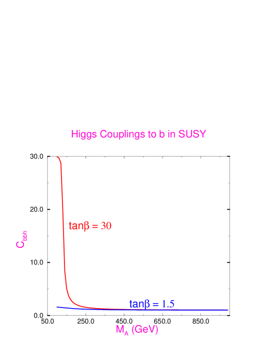
Figure 33: Coupling of the lightest Higgs boson to charge $-1/3$ quarks. The value $C_{bbh}=1$ corresponds to the Standard Model coupling of the Higgs boson to charge $-1/3$ quarks.

There are many analyses$\!{}^{{\bf?}}$ which include a variety of two-loop effects, renormalization group effects, etc., but the important point is that for given values of $\tan\beta$ and the squark masses, there is an upper bound on the lightest neutral Higgs boson mass. For large values of $\tan\beta$ the limit is relatively insensitive to the value of $\tan\beta$ and with a squark mass less than about $1~{}TeV$, the upper limit on the Higgs mass is about $110~{}GeV$ if mixing in the top squark sector is negligible ($A_{T}\sim 0$). For large mixing, this limit is raised to around $130~{}GeV$.

• The minimal supersymmetric model predicts a neutral Higgs boson with a mass less than around $130~{}GeV$.

Such a mass scale may be accessible at LEP2, an upgraded Tevatron or the LHC and provides a definitive test of the MSSM.

In a more complicated supersymmetric model with a richer Higgs structure, the upper bound on the lightest Higgs boson mass will be changed. However, the requirement that the Higgs self coupling remain perturbative up to the Planck scale gives an upper bound on the lightest supersymmetric Higgs boson of around $150~{}GeV$ in all models with only singlets and doublets of Higgs bosons.$\!{}^{{\bf?}}$ This is a very strong statement. It implies that either there is a relatively light Higgs boson or else there is some new physics between the weak scale and the Planck scale which causes the Higgs couplings to become non-perturbative.

Another feature of the MSSM is that the fermion- Higgs couplings are no longer strictly proportional to mass. From the superpotential can be found both the scalar potential and the Yukawa interactions of the fermions with the scalars:

$${\cal L}_{W}=-\sum_{i}\mid{\partial W\over\partial z_{i}}\mid^{2}-{1\over 2}\sum_{ij}\biggl{[}{\overline{\psi}}_{iL}{\partial^{2}W\over\partial z_{i}\partial z_{j}}\psi_{j}+{\rm h.c.}\biggr{]},$$ (200)

where $z_{i}$ is a chiral superfield. This form of the Lagrangian is dictated by the supersymmetry and by the requirement that it be renormalizable. To obtain the interactions, we take the derivatives of $W$ with respect to the superfields, $z_{i}$, and then evaluate the result in terms of the scalar component of $z_{i}$.

The usual approach is to write the most general $SU(3)\times SU(2)_{L}\times U(1)_{Y}$ invariant superpotential with arbitrary coefficients for the interactions,

$$W = \epsilon_{ij}\mu{\hat{H}}_{1}^{i}{\hat{H}}_{2}^{j}+\epsilon_{ij}\biggl{[}\lambda_{L}{\hat{H}}_{1}^{i}{\hat{L}}^{cj}{\hat{E}}^{c}+\lambda_{D}{\hat{H}}_{1}^{i}{\hat{Q}}^{j}{\hat{D}}^{c}+\lambda_{U}{\hat{H}}_{2}^{j}{\hat{Q}}^{i}{\hat{U}}^{c}\biggr{]}$$ (201)

$$+\epsilon_{ij}\biggl{[}{\lambda_{1}}{\hat{L}}^{i}{\hat{L}}^{j}{\hat{E}}^{c}+\lambda_{2}{\hat{L}}^{i}{\hat{Q}}^{j}{\hat{D}}^{c}\biggr{]}+\lambda_{3}{\hat{U}}^{c}{\hat{D}}^{c}{\hat{D}}^{c},$$

(where $i,j$ are $SU(2)$ indices). We have written the superpotential in terms of the fields of the first generation. In principle, the $\lambda_{i}$ could all be matrices which mix the interactions of the $3$ generations.

The terms in the square brackets proportional to $\lambda_{L}$, $\lambda_{D}$, and $\lambda_{U}$ give the usual Yukawa interactions of the fermions with the Higgs bosons from the term

$${\overline{\psi}}_{i}\biggl{(}{\partial^{2}W\over\partial z_{i}\partial z_{j}}\biggr{)}\psi_{j}.$$ (202)

Hence these coefficients are determined in terms of the fermion masses and the vacuum expectation values of the neutral members of the scalar components of the Higgs doublets and are not free parameters at all.

It is convenient to write the couplings for the neutral Higgs bosons to the fermions in terms of the Standard Model Higgs couplings,

$${\cal L}=-{gm_{i}\over 2M_{W}}\biggl{[}C_{ffh}{\overline{f}}_{i}f_{i}h+C_{ffH}{\overline{f}}_{i}f_{i}H+C_{ffA}{\overline{f}}_{i}\gamma_{5}f_{i}A\biggr{]},$$ (203)

where $C_{ffh}$ is $1$ for a Standard Model Higgs boson. The $C_{ffi}$ are given in Table 5 and plotted in Figs. 33 and 34 as a function of $M_{A}$. We see that for small $M_{A}$ and large $\tan\beta$, the couplings of the neutral Higgs boson to fermions can be significantly different from the Standard Model couplings; the $b$-quark coupling becomes enhanced, while the $t$-quark coupling to the lightest Higgs boson is suppressed. When $M_{A}$ becomes large the Higgs-fermion couplings approach their standard model values, $C_{ffh}\rightarrow 1$. In fact even for $M_{A}\sim 300~{}GeV$, the Higgs-fermion couplings are very close to their Standard Model values.

Table 5: Higgs Boson Couplings to fermions $f$ $C_{ffh}$ $C_{ffH}$ $C_{ffA}$ $u$ ${\cos\alpha\over\sin\beta}$ ${\sin\alpha\over\sin\beta}$ $\cot\beta$ $d$ $-{\sin\alpha\over\cos\beta}$ ${\cos\alpha\over\cos\beta}$ $\tan\beta$

Figure 34: Coupling of the lightest Higgs boson to charge $2/3$ quarks. The value $C_{tth}=1$ yields the Standard Model coupling of the Higgs boson to charge $2/3$ quarks.

The Higgs boson couplings to gauge bosons are fixed by the $SU(2)_{L}\times U(1)$ gauge invariance. Some of the phenomenologically important couplings are:

$$Z^{\mu}Z^{\nu}h: {igM_{Z}\over\cos\theta_{W}}\sin(\beta-\alpha)g^{\mu\nu}$$

$$Z^{\mu}Z^{\nu}H: {igM_{Z}\over\cos\theta_{W}}\cos(\beta-\alpha)g^{\mu\nu}$$

$$W^{\mu}W^{\nu}h: igM_{W}\sin(\beta-\alpha)g^{\mu\nu}$$

$$W^{\mu}W^{\nu}H: igM_{W}\cos(\beta-\alpha)g^{\mu\nu}$$

$$Z^{\mu}h(p)A(p^{\prime}): {g\cos(\beta-\alpha)\over 2\cos\theta_{W}}(p+p^{\prime})^{\mu}$$

$$Z^{\mu}H(p)A(p^{\prime}): -{g\sin(\beta-\alpha)\over 2\cos\theta_{W}}(p+p^{\prime})^{\mu}\quad.$$ (204)

We see that the couplings of the Higgs bosons to the gauge bosons all depend on the same angular factor, $\beta-\alpha$. The pseudoscalar, $A^{0}$, has no tree level coupling to pairs of gauge bosons. The angle $\beta$ is a free parameter while the neutral Higgs mixing angle, $\alpha$, which enters into many of the couplings, can be found at leading logarithm in terms of $M_{A}$ and $\beta$:

$$\tan 2\alpha={(M_{A}^{2}+M_{Z}^{2})\sin 2\beta\over(M_{A}^{2}-M_{Z}^{2})\cos 2\beta+\epsilon_{h}/\sin^{2}\beta}\quad.$$ (205)

With our conventions, $-{\pi\over 2}\leq\alpha\leq 0$. It is clear that the couplings of the neutral scalars to vector bosons ($V=W^{\pm},Z$) are suppressed relative to those of the standard model

$$g^{2}_{H_{1}VV}+g^{2}_{H_{2}VV}=g^{2}_{HVV}(SM),$$ (206)

where $g_{HVV}$ is the coupling of the Higgs boson to vector bosons. Because of this sum rule, the $WW$ scattering production mechanism tends not to be as important in supersymmetric models as in the Standard Model.

A complete set of couplings for the Higgs bosons (including the charged and pseudoscalar Higgs) at tree level can be found in Ref. 1. These couplings completely determine the decay modes of the supersymmetric Higgs bosons and their experimental signatures. The important point is that (at lowest order) all of the couplings are completely determined in terms of $M_{A}$ and $\tan\beta$. When radiative corrections are included there is a dependence on the squark masses and the mixing parameters in the mass matrices. This dependence is explored in detail in Ref. 34.

It is an important feature of the MSSM that for large $M_{A}$, the Higgs sector looks exactly like that of the Standard Model. As $M_{A}\rightarrow\infty$, the masses of the charged Higgs bosons, $H^{\pm}$, and the heavier neutral Higgs, $H$, become large leaving only the lighter Higgs boson, $h$, in the spectrum. In this limit, the couplings of the lighter Higgs boson, $h$, to fermions and gauge bosons take on their Standard Model values. We have,

$$\sin(\beta-\alpha) \rightarrow 1~{}{\hbox{for}}~{}M_{A}\rightarrow\infty$$

$$\cos(\beta-\alpha) \rightarrow 0\quad.$$ (207)

From Eq. 204, we see that the heavier Higgs boson, $H$, decouples from the gauge bosons in the heavy $M_{A}$ limit, while the lighter Higgs boson, $h$, has Standard Model couplings. The Standard Model limit is also rapidly approached in the fermion-Higgs couplings for $M_{A}>300~{}GeV$. In the limit of large $M_{A}$, it will thus be exceedingly difficult to differentiate a supersymmetric Higgs sector from the Standard Model Higgs boson.

• The supersymmetric Higgs sector with large $M_{A}$ looks like the Standard Model Higgs sector.

In this case, it will be difficult to discover supersymmetry through the Higgs sector. Instead, it will be necessary to find some of the other supersymmetric partners of the observed particles.

At a hadron collider, the neutral Higgs bosons of a supersymmetric model can be searched for using many of the same techniques as in the Standard Model.$\!{}^{{\bf?},{\bf?}}$ For most choices of the parameter space, gluon fusion is the dominant production mechanism. In the Standard Model, it was only the top quark contribution to gluon fusion which was important. In a supersymmetric model, however, the coupling to the $b$ quark can be important for small values of $\cos\beta$, as can be seen from Table 5.

Supersymmetric models have a rich particle spectrum in which to search for evidence of the Higgs mechanism. The various decays such as $h,H\rightarrow\gamma\gamma$, $H^{+}\rightarrow l^{+}\nu$, $A^{0}\rightarrow\tau^{+}\tau^{-}$, etc, are sensitive to different regions in the $M_{A}-\tan\beta$ parameter space. It takes the combination of many decay channels in order to be able to cover the parameter space completely with out any holes. Discussions of the capabilities of the LHC detectors to experimentally observe evidence for the Higgs bosons of supersymmetric models can be found in the ATLAS$\!{}^{{\bf?}}$ and CMS$\!{}^{{\bf?}}$ studies. An upgraded Tevatron will also have the capability to obtain meaningful limits on the symmetry breaking sector of a supersymmetric model.$\!{}^{{\bf?}}$

Both the Tevatron and the LEP and LEP2 colliders have searched for the Higgs bosons and other new particles occuring in a SUSY model and have ruled out large portions of the $tan\beta$- $M_{A}$ parameter space.$\!{}^{{\bf?}}$

12 Conclusions

Table 6: Higgs Mass Reach of Future Accelerators Accelerator Luminosity Higgs Mass Reach LEP2 ($192~{}GeV$) $150~{}pb^{-1}$ $95~{}GeV$ Tevatron $5-10~{}fb^{-1}$ $80-100~{}GeV$ TEV-33 $25-30~{}fb^{-1}$ $120~{}GeV$ LHC $100~{}fb^{-1}$ $800~{}GeV$ NLC ($500~{}GeV$) $50~{}fb^{-1}$ $350~{}GeV$

Our current experimental knowledge of the Standard Model Higgs boson gives only the limits $M_{h}>90~{}GeV$ and $M_{h}<280~{}GeV$ from direct search experiments and precision measurements at the LEP and LEP2 experiments. From here, we must wait until the advent of an upgraded Tevatron and the LHC for further limits. Through the decay $h\rightarrow\gamma\gamma$ and the production process $pp\rightarrow Zl^{+}l^{-}$, the LHC will probe the mass region between $100<M_{h}<180~{}GeV$, while the Tevatron is sensitive to $M_{h}<130~{}GeV$ with $30~{}fb^{-1}$ through the $Wh$ production process. For the higher mass region, $180<M_{h}<800~{}GeV$, the LHC will be able to see the Higgs boson through the gold plated decay mode, $h\rightarrow ZZ\rightarrow l^{+}l^{-}l^{+}l^{-}$. The expected sensitivity of future colliders is summarized in Table 6.$\!{}^{{\bf?}}$

One of the important yardsticks for all current and future accelerators is their ability to discover (or to definitively exclude) the Higgs boson of the Standard Model. We hope that at the time of the LHC, we will be able to probe all mass scales up to $M_{h}\sim 800~{}GeV$. Having found the Higgs boson, the next goal will be to determine if it is a Standard Model Higgs boson, or a Higgs boson of some more complicated theory such as the MSSM.

If the Higgs boson is not found below this mass scale then we are in the regime where perturbative unitarity has broken down and we are led to the exciting conclusion that there must be new physics beyond the Standard Model waiting to be discovered.

References

- [1] J. Gunion, H. Haber, G. Kane, and S. Dawson, The Higgs Hunters Guide, (Addison-Wesley, Menlo Park, 1990).
- [2] Similar material can be found in J. Bagger, Physics Beyond the Standard Model, lectures given at the 1991 TASI summer school, Boulder, CO, 2-28 June, 1991, (World Scientific, Singapore, 1992); S. Dawson, Introduction to the Physics of Higgs Bosons, lectures given at the 1994 TASI summer school, Boulder, CO, 29 May -24 June, 1994, (World Scientific, Singapore, 1994), hep-ph/9411325; A. Djouadi, Int. J. Mod. Phys. A10 (1995) 1; R. Chivukula, Models of Electroweak Symmetry Breaking: Course, lectures given at the Les Houches Center of Physics, Les Houches, France, 16-26 June, 1998, hep-ph/9803219; M. Spira and P. Zerwas, Electroweak Symmetry Breaking and Higgs Physics, lectures given at the International University School of Nuclear and Particle Physics, Schladming, Austria, 1-8 March 1997, hep-ph/9803257.
- [3] An introduction to the Standard Model can be found in C. Quigg, Gauge Theories of the Strong, Weak, and Electromagnetic Interactions, (Benjamin-Cummings, Reading, MA., 1983).
- [4] E. Abers and B. Lee, Phys. Rep. 9 (1975) 1.
- [5] P. W. Higgs, Phys. Rev. Lett. 13 (1964)508; Phys. Rev. 145 (1966) 1156; F. Englert and R. Brout, Phys. Rev. Lett. 13 (1964) 321; G. S. Guralnik, C. R. Hagen, and T. Kibble, Phys. Rev. Lett. 13 (1965) 585; T. Kibble, Phys. Rev. 155 (1967) 1554.
- [6] S. Glashow, Nucl. Phys. 22 (1961) 579; S. Weinberg, Phys. Rev. Lett. 19 (1976) 1264; A. Salam, in Elementary Particle Theory, ed. N. Svartholm (Almqvist and Wiksells, Stockholm, 1969), p. 367.
- [7] K. Wilson, Phys. Rev. B4 (1971) 3184; K. Wilson and J. Kogut, Phys. Rep. 12 (1974) 75; R. Dashen and H. Neuberger, Phys. Rev. Lett. 50 (1983) 1897; P. Hasenfratz and J. Nager, Z. Phys. C37 (1988); J. Kuti, L. Lin, and Y. Shen, Phys. Rev. Lett. 61 (1988) 678; M. Luscher and P. Weisz, Phys. Lett. B212 (1988) (472).
- [8] R. Chivukula and E. Simmons, Phys. Lett. B388 (1996) 788.
- [9] M. Quiros, Perspectives in Higgs Physics, Ed. G. Kane, (World Scientific, Singapore, 1997).
- [10] A. Hasenfratz, Quantum Fields on the Computer, Ed. M. Creutz, (World Scientific, Singapore, 1992),p. 125.
- [11] T. Cheng, E. Eichten and L. Li, Phys. Rev. D9 (1974) 2259; B. Pendleton and G. Ross, Phys. Lett. B98 (1981) 291; C. Hill, Phys. Rev. D24 (1981) 691; J. Bagger, S. Dimopoulos and E. Masso, Nucl. Phys. B253 (1985) 397; M. Beg, C. Panagiotakopoulos, and A. Sirlin, Phys. Rev. Lett. 52 (1984) 883; M. Duncan, R. Philippe, and M. Sher, Phys. Lett. B153 (1985) 165; K. Babu and E. Ma, Phys. Rev. Lett. 55 (1985) 3005.
- [12] N. Cabibbo et.al., Nucl. Phys. B158 (1979) 295.
- [13] A. Linde, JETP Lett 23 (1976) 64; Phys. Lett. B62 (1976) 435; S. Weinberg, Phys. Rev. Lett. 36 (1976) 294; S. Coleman and E. Weinberg, Phys. Rev. D7 (1973) 188.
- [14] M. Lindner, M. Sher, and H. Zaglauer, Phys. Lett. B228 (1989) 139; C. Ford et. al., Nucl. Phys. B395 (1993) 62; M. Sher, Phys. Rep. 179 (1989)274; F. del Aguila, M Martinez, M. Quiros, Nucl. Phys. B381 (1992) 451; J. Casas, J. Espinosa, and M. Quiros, Phys. Lett. B324 (1995) 171; Phys. Lett. B382 (1996) 374; J. Espinosa and M. Quiros, Phys. Lett. B353 (1995) 257.
- [15] M. Sher, Phys. Lett. B317 (1993)159; addendum, B331 (1994) 448.
- [16] W. Marciano and A. Sirlin, Phys. Rev. Lett. 46 (1981) 163; W. Marciano, S. Sarantakos, and A. Sirlin, Nucl. Phys. B217 (1988) 84.
- [17] T. Appelquist and C. Bernard, Phys. Rev. D22 (1980) 200; A. Longhitano, Nucl. Phys. B188 (1981) 118; T. Appelquist and G. Wu, Phys. Rev. D51 (1995) 240.
- [18] M. Veltman, Acta. Phys. Pol. B8 (1977) 475.
- [19] M. Einhorn and J. Wudka, Phys. Rev. D39 (1989) 2758.
- [20] D. Karlen, results presented at XXIX International Conference on High Energy Physics, Vancouver, Canada, July 23-29, 1998.
- [21] M. Spira, Fortsch. Phys. 46 (1998) 203.
- [22] E. Braaten and J. Leveille, Phys. Rev. D22 (1980) 715; and M. Drees and K. Hikasa, Phys. Lett. B240 (1990) 455.
- [23] K. Melnikov, Phys. Rev. D53 (1996) 5020.
- [24] A. Djouadi and P. Gambino, Phys. Rev. Lett. 73 (1994) 2528.
- [25] A. Djouadi, J. Kalinowski, and M. Spira, Comput. Phys. Comm. 108 (1998) 56.
- [26] W.-Y. Keung and W. Marciano, Phys. Rev. D30 (1984) 248.
- [27] T. Inami, T. Kubota, and Y. Okada, Z. Phys. C18 (1983) 69; M. Spira, A. Djouadi, D. Graudenz, and P. Zerwas, Nucl. Phys. B453 (1995) 17.
- [28] R. Cahn, M. Chanowitz, and N. Fleishon, Phys. Lett. B82 (1979)113; G. Gamberini, G. Giudice and G. Ridolfi, Nucl. Phys. B292 (1987) 237.
- [29] A. Vainshtein, M. Voloshin, V. Sakharov, and M. Shifman, Sov. J. Nucl. Phys. 30 (1979) 711.
- [30] S. Dawson and R. Kauffman, Phys. Rev. D49 (1993) 2298; A. Djouadi, M. Spira, and P. Zerwas, Phys. Lett. B311 (1993) 255.
- [31] B. Ioffe and V. Khoze, Sov. J. Part. Nucl. Phys. 9 (1978) 50.
- [32] B. Kniehl, Phys. Rep. 240C (1994) 211.
- [33] F. Berends, W. van Neerven, and G. Burgers, Nucl. Phys. B297 (1988) 429; erratum B304 (1988) 921.
- [34] M. Carena and P. Zerwas, Higgs Physics, CERN Yellow Report, CERN-96-01, hep-ph/9602250.
- [35] V. Barger, M. Berger, J. Gunion, and T. Han, Phys. Rev. Lett. 78 (1997) 3991.
- [36] V. Barger, K. Cheung, A. Djouadi, B. Kniehl, and P. Zerwas, Phys. Rev. D49 (1994) 49.
- [37] W. Kilian, M. Kramer, and P. Zerwas, Phys. Lett. B381 (1996) 243.
- [38] F. Wilczek, Phys. Rev. Lett. 39 (1977) 1304; J. Ellis et.al., Phys. Lett. 83B (1979) 339; H. Georgi et. al., Phys. Rev. Lett. 40 (1978) 692; T. Rizzo, Phys. Rev. D22 (1980) 178.
- [39] M. Spira, A. Djouadi, D. Graudenz, and P. Zerwas, Nucl. Phys. B453 (1995) 17.
- [40] S. Dawson, Nucl. Phys. B359 (1991) 283.
- [41] A. Vainshtein et.al., Sov. J. Nucl. Phys.; M. Voloshin, Sov. J. Nucl. Phys. B44 (1986) 478.
- [42] R. Kauffman, Phys. Rev. D45 (1992) 1512.
- [43] LOI of the ATLAS Collaboration, CERN/LHCC/92-4, Oct., 1992.
- [44] LOI of the CMS Collaboration, CERN/LHCC/92-3, Oct., 1992.
- [45] F. Paige, Supersymmetry Signatures at the Cern LHC, lectures given at the 1997 TAS7 summer school, Boulder, CO, 2-28 June, 1997, (World Scientific, Singapore, 1998).
- [46] P. Agrawal and S. Ellis, Phys. Lett. B229 (1989) 145.
- [47] J. Gunion, G. Kane, and J. Wudka, Nucl. Phys. B299 (1988) 231.
- [48] K. Ellis , Nucl. Phys. B297(1988) 221.
- [49] D. Rainwater, D. Zeppenfeld, and K. Hagiwara, hep-ph/9808468.
- [50] W. Marciano, A. Stange, and S. Willenbrock, Phys. Rev. D49 (1994) 1354; Phys. Rev. D50 (1994) 4491.
- [51] T. Han and S. Willenbrock, Phys. Lett. B273 (1991) 167.
- [52] Future Electroweak Physics at the Fermilab Tevatron; Report of the TeV 2000 Study Group, Ed. D. Amidei and R. Brock, Fermilab-PUB-96-082, April, 1996.
- [53] S. Mrenna and C. P. Yuan, Phys. Lett. B416 (1998) 200.
- [54] S. Kim, S. Kuhlmann, and W. -M. Yao, in Proceedings of the 1996 DPF/DPB Summer Study on New Directions for High Energy Physics, 1996; W. - M. Yao, in Proceedings of the 1996 DPF/DPB Summer Study on New Directions for High Energy Physics, (Snowmass, Colorado, July, 1996.
- [55] S. Dawson, Nucl. Phys. B249 (1985) 42; G. Kane, W. Repko, and W. Rolnick, Phys. Lett B148 (1984) 367; M Chanowitz and M. Gaillard, Phys. Lett. B142 (1984) 85.
- [56] S. Brodsky, T. Kinoshita, and H. Terazawa, Phys. Rev. D4 (1971) 1532.
- [57] U. Baur and E. Glover, Nucl. Phys. B347 (1990) 12; Phys. Rev. D44 (1991) 99.
- [58] R. Cahn et. al. Phys. Rev. D35 (1987) 1626; V. Barger, T. Han, and R. Phillips, Phys. Rev. D37 (1988) 2005; J. Gunion and M. Soldate, Phys. Rev. D34 (1986) 826.
- [59] A Djouadi, D. Haidt, B. Kniehl, B. Mele, and P. Zerwas, Proceedings of Collisions at : The Physics Potential, (Munich-Annecy-Hamburg), ed. P.Zerwas, DESY 92-123A.
- [60] S. Dawson and J. Rosner, Phys. Lett., B148 (1984) 497.
- [61] A. Djouadi, J. Kalinowski, and P. Zerwas, Zeit. fur Phy. C54 (1992) 255; K. Gaemers and G. Gounaris, Phys. Lett. B77 (1978) 379.
- [62] S. Dawson and L. Reina, hep-ph/9808443; S. Dittmaier et.al., hep-ph/9808433.
- [63] W. Marciano and S. Willenbrock, Phys. Rev. D37 (1988) 2509.
- [64] B. Lee, C. Quigg, and H. Thacker, Phys. Rev. D16 (1977) 1519; D. Dicus and V. Mathur, Phys. Rev. D7 (1973) 3111.
- [65] M. Duncan, G. Kane, and W. Repko, Nucl. Phys. B272 (1986) 517.
- [66] J. Cornwall, D. Levin, and G. Tiktopoulos, Phys. Rev. D10 (1974) 1145; D11 (1975) 972E; B. Lee, C. Quigg, and H. Thacker, Phys. Rev. D16 (1977) 1519; M. Chanowitz and M. Gaillard, Nucl. Phys. B261 (1985) 379; Y.-P. Yao and C. Yuan, Phys. Rev. D38 (1988) 2237; J. Bagger and C. Schmidt, Phys. Rev. D41 (1990) 264; H. Veltman, Phys. Rev. D41 (1990) 2294.
- [67] S. Dawson and S. Willenbrock, Phys. Rev. D40 (1989); M. Veltman and F. Yndu rain, Nucl. Phys. B163 (1979) 402.
- [68] M. Chanowitz and M. Gaillard, Nucl. Phys. B261 (1985) 379.
- [69] M. Chanowitz, H. Georgi, and M. Golden, Phys. Rev. Lett. 57 (1986) 2344; Phys. Rev.D36 (1987) 1490.
- [70] J. Gasser and H. Leutwyler, Ann. Phys. 158 (1984) 142; Nucl. Phys. B250 (1985) 465.
- [71] S. Weinberg, Phys. Rev. Lett. 17 (1966) 616.
- [72] S. Dawson and G. Valencia, Nucl. Phys. B439 (1995) 3.
- [73] S. Alam, S. Dawson and R. Szalapski, Phys. Rev. D57 (1998) 1577.
- [74] R. Szalapski, Phys. Rev. D57 (1998) 5519; A. De Rujula, M. Gavela, P. Hernandez, and E. Masso, Nucl. Phys. B384 (1992)3.
- [75] M. Peskin and T. Takeuchi, Phys. Rev. Lett. 65 (1990) 964; D. Kennedy and B. Lynn, Nucl. Phys. B322 (1989) 1.
- [76] K. Hagiwara, S. Ishihara, R. Szalapski, and D. Zeppenfeld, Phys. Rev. D48 (1993) 2182.
- [77] A. Falk, M. Luke, and E. Simmons, Nucl. Phys. B365 (1991) 523.
- [78] J. Bagger, S. Dawson, and G. Valencia, Nucl. Phys. B399 (1993) 364.
- [79] J. Bagger et.al., Phys. Rev. D49 (1994) 1246; R. Chivukula, M. Dugan, and M. Golden, Ann. Rev. Nucl. Part. Sci. 45 (1995) 255.
- [80] J. Donoghue, C. Ramirez, and G. Valencia, Phys. Rev. D38 (1988) 2195; Phys. Rev. D39 (1989) 1947; M. Herrero and E. Morales, Nucl. Phys. B418 (1993) 364.
- [81] T. Appelquist and J. Carrazone, Phys. Rev. D11 (1975) 2856.
- [82] See lectures in this school by N. Arkani-Hamed.
- [83] For a review of SUSY phenomenology, see G. Kane and H. Haber, Phys. Rep. 117C (1985) 75; H. Haber, TASI 1992 (World Scientific, Singapore, 1992).
- [84] J. Bagger and J. Wess, Supersymmetry and Supergravity (Princeton University Press, 1983).
- [85] G. Kane, H. Haber, and T. Stirling, Nucl. Phys. B161 (1979) 493.
- [86] H. Haber and R. Hempfling, Phys. Rev. Lett. 66 (1991) 1815; J. Ellis, G. Ridolfi and F. Zwirner, Phys. Lett. B257 (1991) 83; M. Berger, Phys. Rev. D41 (1990) 225; Y. Okada, M. Yamaguchi, and T. Yanagida, Prog. Theor. Phys. Lett. 85 (1991)1; M. Carena, M. Quiros, and C. Wagner, Nucl. Phys. B461 (1996) 407.
- [87] G. Kane, C. Kolda,M. Quiros, and J. Wells, Phys. Rev. Lett. 70 (1993) 2686.
- [88] M. Carena, S. Mrenna, and C. Wagner, ANL-HEP-PR-98-54, hep-ph/9808312.
- [89] A. Djouadi, report of the MSSM working group for the Workshop on GDR-Supersymmetry, hep-ph/9901246; Daniel Treille, results presented at XXIX International Conference on High Energy Physics, Vancouver, Canada, July 23-29, 1998.
- [90] H. Haber, et. al., in Proceedings of the 1996 DPF/DPB Summer Study on New Directions for High Energy Physics, 1996.