Couplings of pions to higher positive parity heavy mesons

Abstract:

We evaluate the couplings of pions in the transitions of positive parity heavy mesons, $(1^{+},2^{+})$ and $(0^{+},1^{+})$, to negative parity ones $(0^{-},1^{-})$ using a technique which is not limited to the soft-pion limit. This is made through a constituent quark-meson model (the CQM model) where the amplitudes are obtained by quark loops with mesons on the external lines. The results are in good agreement with experimental data.

1 Introduction

Positive parity mesons comprising one heavy quark are the object of a wide experimental search [1] and this demands a deeper theoretical understanding of processes involving these states. A theoretical description within QCD can be attempted at present only by numerical simulations or by the use of QCD sum rules. However much of what is known about QCD can also be described by using an effective Lagrangian, encoding the symmetries and dynamical properties of the theory with a limited number of parameters. This is possible because the use of expansion parameters, such as the energy or the heavy quark mass, makes sense in some limited kinematical regions, whereas in principle the effective Lagrangian description would require an infinite number of operators, and correspondingly an infinite number of free parameters. The effective Lagrangian approach is usually simple enough to allow for analytical calculations, thus giving the opportunity to see in detail the interplay between symmetries and dynamical information introduced into the model.

We are interested here in a constituent quark-meson model (the CQM model [2, 3]) in the intermediate range of energies between the confinement scale and the 1 GeV region. In this model both quark and meson effective fields are present. In the following we extend the analysis described in [2, 3] to the study of strong decays $D_{2}^{*}\to D\pi$, $D_{1}^{*}\to D\pi$. Here the states $D_{2}^{*}$, $D_{1}^{*}$ are the observed 2460 and 2420 charmed positive parity mesons. We also generalise the computation of strong decays $D_{1}^{*\prime}\to D\pi$, $D_{0}\to D^{*}\pi$ made in [2] avoiding the soft-pion-approximation used there (the $D_{1}^{*\prime}$, $D_{0}$ states have $J^{P}=1^{+}$, $0^{+}$).

Our strategy is to consider a quark-meson Lagrangian where transition amplitudes are represented by diagrams with heavy mesons attached to loops containing heavy and light constituent quarks. The effective meson-quark vertices emerge as a result of path integral bosonization of an underlying 4-quark Nambu-Jona-Lasinio (NJL) interaction. Our results are encouraging especially in consideration of the technical simplicity that the method offers in comparison to other available approaches, such as for instance in [4].

2 The model

A short presentation of the CQM model is in order; for a full account see [2] and references therein. The model is an effective field theory containing a quark-meson Lagrangian incorporating heavy-quark symmetries [5]. For our purposes this Lagrangian can be divided into two parts:

$${\cal L}={\cal L}_{\ell\ell}+{\cal L}_{h\ell}.$$ (1)

The first term involves only the light quark degrees of freedom, $\chi$, and the pseudoscalar light mass octet. At the lowest order in a derivative expansion one has:

$${\cal L}_{\ell\ell}={\bar{\chi}}(iD^{\mu}\gamma_{\mu}+{\cal A}^{\mu}\gamma_{\mu}\gamma_{5})\chi-m{\bar{\chi}}\chi+{f_{\pi}^{2}\over 8}\partial_{\mu}\Sigma^{\dagger}\partial^{\mu}\Sigma\;.$$ (2)

Apart from the mass term, ${\cal L}_{\ell\ell}$ is chiral invariant. Here $D_{\mu}=\partial_{\mu}-i{\cal V}_{\mu}$, $\xi=\exp(i\pi/f_{\pi})$, $\Sigma=\xi^{2}$, $f_{\pi}=130$ MeV. $\pi$ is the $3\times 3$ matrix representing the flavour $SU(3)$ octet of pseudoscalar mesons and the explicit expressions for ${\cal V}^{\mu}$ and ${\cal A}^{\mu}$ are:

$${\cal V}^{\mu} = {1\over 2}(\xi^{\dagger}\partial^{\mu}\xi+\xi\partial^{\mu}\xi^{\dagger})$$

$${\cal A}^{\mu} = {i\over 2}(\xi^{\dagger}\partial^{\mu}\xi-\xi\partial^{\mu}\xi^{\dagger})~{}.$$ (3)

As one can see by expanding the exponential of the pseudoscalar mesons $\xi$, ${\cal V}^{\mu}$ generates couplings of an even number of pseudoscalar mesons to the ${\bar{\chi}}\chi$ pair, while ${\cal A}^{\mu}$ gives an odd number of $\pi$ fields.

The effective Lagrangian containing heavy and light quarks together with meson fields is:

$${\cal L}_{h\ell} = {\bar{Q}}_{v}iv\cdot\partial Q_{v}-\left[{\bar{\chi}}({\bar{H}}+{\bar{S}}+i{\bar{T}}_{\mu}{D^{\mu}\over{\Lambda_{\chi}}})Q_{v}+h.c.\right]$$ (4)

$$+ \frac{1}{2G_{3}}{\mathrm{Tr}}[({\bar{H}}+{\bar{S}})(H-S)]+\frac{1}{2G_{4}}{\mathrm{Tr}}[{\bar{T}}_{\mu}T^{\mu}]~{}~{}.$$

Here $Q_{v}$ is the effective heavy quark field of Heavy Quark Effective Theory (HQET) [5], $\Lambda_{\chi}$ is the momentum scale characterising the convergence of the derivative expansion, usually taken as the chiral symmetry breaking scale $\Lambda_{\chi}\simeq 1$ GeV, and $H$, $S$, $T$ fields are the effective meson fields discussed in [6] which, in the explicit matrix representation, have the form:

$$H = \frac{1+v\hskip-5.20601pt\lower 0.34723pt\hbox to5.20601pt{\hss\sl/\/\hss}}{2}\;[P_{\mu}^{*}\gamma^{\mu}-P\gamma_{5}]$$ (5)

$$S = {{1+v\hskip-5.20601pt\lower 0.34723pt\hbox to5.20601pt{\hss\sl/\/\hss}}\over 2}[P_{1\mu}^{*\prime}\gamma^{\mu}\gamma_{5}-P_{0}]$$ (6)

$$T^{\mu} = {\frac{1+v\hskip-5.20601pt\lower 0.34723pt\hbox to5.20601pt{\hss\sl/\/\hss}}{2}}\left[P_{2}^{*\mu\nu}\gamma_{\nu}-\sqrt{\frac{3}{2}}P^{*}_{1\nu}\gamma_{5}\left(g^{\mu\nu}-\frac{1}{3}\gamma^{\nu}(\gamma^{\mu}-v^{\mu})\right)\right]\;.$$ (7)

Here $P,P^{*}_{\mu}$ etc. are annihilation operators normalised in the following way:

$$\langle 0|P|Q{\bar{q}}(0^{-})\rangle = \sqrt{M_{H}}$$ (8)

$$\langle 0|{P^{*}}^{\mu}|Q{\bar{q}}(1^{-})\rangle = \epsilon^{\mu}\sqrt{M_{H}}$$ (9)

$$\langle 0|{P_{2}^{*}}^{\mu\nu}|Q{\bar{q}}(2^{+})\rangle = \epsilon^{\mu\nu}\sqrt{M_{T}}$$ (10)

$H,S$ and $T^{\mu}$ describe respectively the $(0^{-},1^{-})$ doublet, the $(0^{+},1^{+})$ doublet $D_{0},D_{1}^{*\prime}$ and the $(1^{+},2^{+})$ doublet $D_{1}^{*},D_{2}^{*}$ that are predicted by HQET. The part in the Lagrangian containing the $T$ field is not directly read from the underlying NJL contact interaction, but it constitutes its expected extension. The coupling constants $G_{3}$, $G_{4}$ and the field renormalization constants $Z_{H},Z_{S},Z_{T}$ are discussed in [2] (for numerical values see below). Another parameter of the model is $\Delta_{H}$, i.e. the difference between the $H$ meson doublet mass and the mass of the heavy quark involved. This parameter is not predicted by the model but, once $\Delta_{H}$ is fixed, the model gives $\Delta_{S}$ (as a result of the dynamical information introduced into the Lagrangian by the underlying NJL contact interaction), while $\Delta_{T}$ is still a free parameter that can be estimated using experimental information. The following table was computed in [2]:

$\Delta_{H}$	$\Delta_{S}$	$\Delta_{T}$
$0.3$	$0.545$	$0.635$
$0.4$	$0.590$	$0.735$
$0.5$	$0.641$	$0.835$

Table 1: $\Delta$ values (in GeV)

We allow for a variation of $\Delta_{H}=0.4\pm 0.1$ GeV, since only this range of values is allowed by the results on semileptonic weak decays (for a discussion see [2]).

The last step necessary to the definition of the model is the choice of a regularization procedure. We use the Schwinger proper time regularization method assuming as UV and IR cut-off $\Lambda\simeq 1.25$ GeV and $\mu\simeq 0.3$ GeV respectively. The former ensures the suppression of large momentum flows through light quark lines in the loops, since the heavy quark carries most of the energy and momentum in the system; the latter, being of order of $\Lambda_{\rm QCD}$, drops the unknown confinement part of the quark interaction (see for example [7]). The regularized form of the heavy quark propagator is:

$$\int d^{4}k_{E}\frac{1}{k_{E}^{2}+m^{2}}\to\int d^{4}k_{E}\int_{1/\Lambda^{2}}^{1/\mu^{2}}ds\;e^{-s(k_{E}^{2}+m^{2})}~{}~{},$$ (11)

where $m$ is the constituent light quark mass, which we take as $m=0.3$ GeV for $u$ and $d$ flavours. An alternative way of cutting off high momenta is proposed in [8].

3 Strong couplings

As shown in [6], transitions $T\to H\pi$ are described by an interaction Lagrangian that in HQET has the the following form:

$${\cal L}=\frac{h_{1}}{\Lambda_{\chi}}{\rm Tr}[{\bar{H}}T^{\mu}(iD_{\mu}{\cal A}\hskip-7.50002pt\lower-0.91666pt\hbox to7.50002pt{\hss\sl/\/\hss})\gamma_{5}]+\frac{h_{2}}{\Lambda_{\chi}}{\rm Tr}[{\bar{H}}T^{\mu}(iD\hskip-8.55695pt\lower-0.91666pt\hbox to8.55695pt{\hss\sl/\/\hss}{\cal A})\gamma_{5}]+h.c.\;,$$ (12)

while for the $S\to H\pi$ transitions we have:

$${\cal L}=ig{\mathrm{Tr}}(\overline{H}H\gamma^{\mu}\gamma_{5}{\cal A}_{\mu})\;+\;\left[ih\;{\mathrm{Tr}}(\overline{H}S\gamma^{\mu}\gamma_{5}{\cal A}_{\mu})\;+\;{\mathrm{h.c.}}\right]$$ (13)

The general amplitudes, for the processes we are interested in, are defined as follows:

$$\langle D^{+}(p^{\prime})\pi^{-}(q)|D_{2}^{*0}(p,\eta)\rangle = ig_{1}\eta^{\mu\nu}q_{\mu}q_{\nu}$$ (14)

$$\langle D^{*+}(p^{\prime},\epsilon)\pi^{-}(q)|D_{2}^{*0}(p,\eta)\rangle = ig_{2}\eta^{\mu\nu}q_{\mu}\epsilon_{\lambda\sigma\nu\tau}\epsilon^{*\lambda}\frac{p^{\sigma}}{m_{T}}q^{\tau}$$ (15)

$$\langle D^{*+}(p^{\prime},\epsilon)\pi^{-}(q)|D_{1}^{*0}(p,\eta)\rangle = ig_{3}\eta_{\nu}\epsilon^{*}_{\sigma}[3q^{\nu}q^{\sigma}+g^{\nu\sigma}(q^{2}-\frac{(p\cdot q)^{2}}{m_{T}})]$$ (16)

$$\langle D^{0}(p^{\prime})\pi^{+}(q)|D_{0}^{+}(p)\rangle = ig_{4}\frac{m_{S}^{2}-m_{H}^{2}}{m_{S}}$$ (17)

$$\langle D^{0}(p^{\prime})\pi^{+}(q)|D^{*+}(p,\epsilon)\rangle = ig_{5}q^{\mu}\epsilon_{\mu}\;,$$ (18)

where we are using the HQET definitions of the symbols $H,S,T$ for labelling mesons masses. The connection with $h_{1},h_{2},g,h$ is:

$$g_{1} = g_{2}=2\sqrt{m_{H}m_{T}}\frac{h^{\prime}}{\Lambda_{\chi}f_{\pi}}$$ (19)

$$g_{3} = \sqrt{\frac{2m_{H}m_{T}}{3}}\frac{h^{\prime}}{\Lambda_{\chi}f_{\pi}}$$ (20)

$$g_{4} = \sqrt{m_{H}m_{S}}\frac{h}{f_{\pi}}$$ (21)

$$g_{5} = \frac{2m_{H}}{f_{\pi}}g~{}~{},$$ (22)

where $h^{\prime}=h_{1}+h_{2}$.

Our method consists in a loop calculation of a diagram such as in Fig. 1 involving a current and two meson states on the external legs. Let us consider the calculation of $T\to H\pi$ , i.e. the determination of $h^{\prime}$.

According to the Feynman rules derived from Eq. (1) and Eq. (12), the loop shown in figure may be written as:

$$-\frac{i}{2}\sqrt{Z_{H}Z_{T}m_{H}m_{T}}q^{\mu}\eta^{\sigma\nu}\frac{iN_{c}}{16\pi^{4}}\int^{\mathrm{reg}}d^{4}k\frac{{\rm Tr}[(k\hskip-5.52084pt\lower-0.97221pt\hbox to5.52084pt{\hss\sl/\/\hss}+m)\gamma_{\mu}\gamma_{5}(k\hskip-5.52084pt\lower-0.97221pt\hbox to5.52084pt{\hss\sl/\/\hss}^{\prime}+m)\gamma_{5}(1+v\hskip-5.20601pt\lower 0.34723pt\hbox to5.20601pt{\hss\sl/\/\hss})\gamma_{\nu}k_{\sigma}]}{(k^{2}-m^{2})[(k+q)^{2}-m^{2}](v\cdot k+\Delta+i\epsilon)}$$ (23)

The computation of the previous expression can be decomposed in simpler expressions involving integrals such as as $Z$, $Z^{\sigma}$, $Z^{\sigma\nu}$, and $Z^{\sigma\nu\lambda}$ (reported in the appendix). The numerators of these integrals are the Lorentz structures $1$, $k^{\sigma}$, $k^{\sigma}k^{\nu}$, $k^{\sigma}k^{\nu}k^{\lambda}$ respectively.

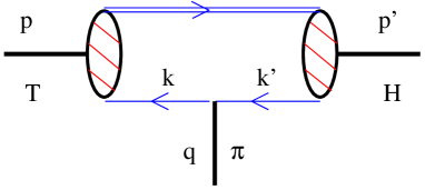
Figure 1: Diagram for the loop calculation of the $T\to H\pi$ coupling $h^{\prime}$ in the constituent quark-meson model.

Once Eq. (23) is calculated, the coupling $h^{\prime}$ may be obtained by matching the previous calculation in the quark-meson loop model Eq. (4) with the expression of the effective Lagrangian, where the only degrees of freedom are heavy and light mesons Eq. (12) and $h^{\prime}=h_{1}+h_{2}$. The same strategy is followed for the evaluation of $h$ and $g$ in Eq. (13). For the $T\to H\pi$ coupling we find:

$$h^{\prime} = \sqrt{Z_{T}Z_{H}}\Big{\{}\frac{m^{2}}{q_{\pi}}\Big{[}I_{2}+\Delta_{T}Z(\Delta_{T})+\frac{1}{2q_{\pi}}(I_{3}(\Delta_{H})-I_{3}(\Delta_{T}))\Big{]}$$ (24)

$$+ P(R_{i}(\Delta_{T}),S_{i}(\Delta_{T}),q_{\pi})\Big{\}}~{},$$

where the polynomial $P(R_{i},S_{i},q_{\pi})$, expressed as a sum of powers of $q_{\pi}$ multiplied by the linear combinations $R_{i}$ and $S_{i}$ of $I_{i}$ and $Z$ integrals, is given in the appendix, together with the expressions for $I_{i}$ and $Z$. The parameter $q_{\pi}$ is $q_{\pi}=v\cdot q$ where $v$ is the velocity of the incoming meson and $q^{\mu}$ is the pion 4-momentum. Consistently with chiral invariance we neglect the pion mass and we write $q^{\mu}=(q_{\pi},0,0,q_{\pi})$ in the decaying particle rest frame. Also, consistently with the effective Lagrangian (12), containing the minimum number of couplings, in the evaluation of Eq. (24) we neglected $O(q_{\pi}^{3})$ terms. Two powers of $q_{\pi}$ have to be kept, since they appear in the D-wave matrix element (14)-(16).

Varying $\Delta_{H}$ in the same range as in Table I, we can evaluate the variation of the field renormalization constants $Z_{H},Z_{S},Z_{T}$ defining the renormalized fields ${\hat{H}}=H/\sqrt{Z_{H}}$, ${\hat{S}}=S/\sqrt{Z_{S}}$ and ${\hat{T}}=T/\sqrt{Z_{T}}$. We only report values of $Z_{H},Z_{S},Z_{T}$ for $\Delta_{H}=0.4$ which are respectively $2.36,1.14,1.07~{}{\rm GeV}^{-1}$ (see [2] for a complete table).

For the strong coupling $S\to H\pi$ we find:

$$h=\sqrt{Z_{S}Z_{H}}\left[R_{1}(\Delta_{S})-R_{2}(\Delta_{S})-\frac{R_{4}(\Delta_{S})}{q_{\pi}}+m^{2}Z(\Delta_{S})\right].$$ (25)

In this calculation we have considered terms only up to the order $O(q_{\pi}^{1})$, to be consistent with the energy expansion for the chiral fields, as explained before; this result goes beyond the soft pion limit approximation (SPL) which is often used in these calculations (see the discussion below). Numerically we find:

$$h^{\prime}=0.65^{+0.45}_{-0.3}\;,$$ (26)

where the error is induced by the variation of $\Delta_{H}$ in the range $0.3-0.5$ GeV. For $h$ we obtain:

$$h=-0.76\pm 0.13\;.$$ (27)

Here we use the mass determination of the $S-$multiplet made in [2] i.e. $2.165\pm 0.05$ GeV. The error in this determination does not contribute significantly to $h$. Note that recent preliminary experimental results by CLEO [9] give a mass of $2.461$ GeV for the broad $1^{+}$ state attributed to the $S$ multiplet. This difference may be understood as a consequence of a ${\cal O}(1/m_{c})$ correction to the mass formula.

Using the preliminary CLEO results for the $1^{+}$ mass in the $S$ multiplet (it affects the pion momentum in (25)), we get:

$$h=-0.56\pm 0.11$$ (28)

which is consistent with the one obtained by QCD sum rules [10]:

$$h=-0.52\pm 0.17\;.$$ (29)

The approach used in this paper to calculate the strong coupling constants outside the SPL is an improvement with respect to [2], where we found $h=-0.85\pm 0.02$ using $q_{\pi}\to 0$ from the very beginning. For $g$, the soft pion limit is instead a very good approximation since the decay $D^{*}\to D\pi$ has a very limited phase space. This is confirmed by the evaluation of $g$ made in [2]:

$$g=0.46\pm 0.04\;.$$ (30)

This value agrees with QCD sum rules calculations [11] and with a result from a relativistic constituent quark model [12], giving $g=0.44\pm 0.16$ and $g=0.40$ respectively.

We conclude by calculating the widths of the $T$ and $S$ states to $H$ plus pion, where the heavy quark is a c quark, since these states are already observed. These two body decay processes, from the chiral heavy meson Lagrangian, were already discussed in [6], to which we refer for more details. Using updated experimental data [13] for the masses in the phase space integrals, and our determination of the coupling $h^{\prime}$, we obtain:

$$\Gamma(D_{2}^{*0}\to D^{+}\pi^{-}) = 4.59\times 10^{7}\frac{h^{\prime 2}}{\Lambda_{\chi}^{2}}MeV=19.4MeV$$ (31)

$$\Gamma(D_{2}^{*0}\to D^{*+}\pi^{-}) = 1.33\times 10^{7}\frac{h^{\prime 2}}{\Lambda_{\chi}^{2}}MeV=5.6MeV$$ (32)

$$\Gamma(D_{1}^{*0}\to D^{*+}\pi^{-}) = 1.47\times 10^{7}\frac{h^{\prime 2}}{\Lambda_{\chi}^{2}}MeV=6.2MeV$$ (33)

in which the central value of $h^{\prime}=0.65$ is used and $f_{\pi}=130$ MeV, $\Lambda_{\chi}=1000$ MeV. The full one pion widths are a factor 1.5 larger than those in the previous formula because of the neutral pion decay channel. As the total $D_{2}^{*0}$ width is dominated by the one pion mode in the chiral heavy meson Lagrangian, one can use the experimental result of $23\pm 5$ MeV to extract an experimental value for $h^{\prime}$ from the previous formula. One obtains a value of 0.51, which is in good agreement with the value of $h^{\prime}$ predicted by our model. From (33) one can also deduce the total one pion width of $D_{1}^{*0}$, $\Gamma=9.3$ MeV, which is only half the measured total with $18.9^{+4.6}_{-3.5}$. However this state can mix with the broader $1^{+}$ state in the $S$ multiplet, the $D_{1}^{\prime}$ or can be affected by significant $1/m_{c}$ corrections [14]. Neglecting this mixing we can compute the width of the $D_{1}^{\prime}$ state by using the preliminary CLEO result for the mass [9] and the computed strong coupling constant $h$ given in (28). We obtain

$$\Gamma(D_{1}^{\prime}\to D^{*}\pi)=240\;{\mathrm{M}eV}~{}~{},$$ (34)

which accounts probably for most of the total $D_{1}^{\prime}$ width due to the limited available phase space. This result can be compared with the preliminary CLEO data for the total width, $290^{+101}_{-79}\pm 26\pm 36$ MeV.

4 Conclusions

In this paper we have investigated the phenomenological implications for excited positive parity heavy mesons of the model proposed in [2]. The work is experimentally relevant at present for the charm states, for which these transitions are seen, and a comparison with theoretical calculations is indeed needed. We have improved the technique for diagrams involving a pion vertex on the light quark line, achieving a determination of the strong couplings of the pion in the processes $S\to H\pi$ which turn out to be very close to the QCD sum rule determinations [10]. Moreover, using a technique which goes beyond the soft-pion-limit approximation, we have calculated the strong coupling of the pion in the transition $T\to H\pi$, where such a limit could not be reliably applied. This coupling is then used to predict, for charmed heavy mesons, the decay widths of the $T$ doublet of states $2^{+}$ and $1^{+}$ to the $H$ states $1^{-}$ and $0^{-}$ plus one pion.

Appendix A Appendix

In the paper we use several integrals that we list in this appendix.

$$I_{1} = \frac{iN_{c}}{16\pi^{4}}\int^{\mathrm{reg}}\frac{d^{4}k}{(k^{2}-m^{2})}={{N_{c}m^{2}}\over{16\pi^{2}}}\Gamma(-1,{{{m^{2}}}\over{{{\Lambda}^{2}}}},{{{m^{2}}}\over{{{\mu}^{2}}}})$$ (35)

$$I_{2} = -\frac{iN_{c}}{16\pi^{4}}\int^{\mathrm{reg}}\frac{d^{4}k}{(k^{2}-m^{2})^{2}}={{N_{c}}\over{16\pi^{2}}}\Gamma(0,{{{m^{2}}}\over{{{\Lambda}^{2}}}},{{{m^{2}}}\over{{{\mu}^{2}}}})$$ (36)

$$I_{3}(\Delta) = -\frac{iN_{c}}{16\pi^{4}}\int^{\mathrm{reg}}\frac{d^{4}k}{(k^{2}-m^{2})(v\cdot k+\Delta+i\epsilon)}$$ (37)

$$= {N_{c}\over{16\,{{\pi}^{{3/2}}}}}\int_{1/{{\Lambda}^{2}}}^{1/{{\mu}^{2}}}{ds\over{s^{3/2}}}\;e^{-s({m^{2}}-{{\Delta}^{2}})}\;\left(1+{\mathrm{erf}}(\Delta\sqrt{s})\right)$$

$$I_{4}(\Delta) = \frac{iN_{c}}{16\pi^{4}}\int^{\mathrm{reg}}\frac{d^{4}k}{(k^{2}-m^{2})^{2}(v\cdot k+\Delta+i\epsilon)}$$ (38)

$$= \frac{N_{c}}{16\pi^{3/2}}\int_{1/\Lambda^{2}}^{1/\mu^{2}}\frac{ds}{s^{1/2}}\;e^{-s(m^{2}-\Delta^{2})}\;[1+{\mathrm{erf}}(\Delta\sqrt{s})]~{}.$$

where $\Gamma$ is the generalised incomplete gamma function and erf is the error function. We also define:

$$Z(\Delta) = \frac{iN_{c}}{16\pi^{4}}\int^{\mathrm{reg}}\frac{d^{4}k}{(k^{2}-m^{2})[(k+q)^{2}-m^{2}](v\cdot k+\Delta+i\epsilon)}$$ (39)

$$= \frac{N_{c}}{16\pi^{3/2}}\int_{1/\Lambda^{2}}^{1/\mu^{2}}\frac{ds}{s^{1/2}}e^{-sm^{2}}\int_{0}^{1}dxe^{s\Delta^{2}(x)}[1+{\mathrm{erf}}(\Delta(x)\sqrt{s})]$$

Where $q^{\mu}=(q_{\pi},0,0,q_{\pi})$ is the pion 4-momentum and $\Delta(x)=\Delta-xq_{\pi}$. We can observe that the soft pion limit of the preceding expression, i.e. the limit $q_{\pi}\to 0$, brings $Z(\Delta)\to I_{4}(\Delta)$ as it should be, (cfr. I). We need another auxiliary integral and some expressions which are linear combination of the integrals listed. They are the following:

$$\Theta = \frac{N_{c}}{16\pi^{2}}\int_{1/\Lambda^{2}}^{1/\mu^{2}}ds\left(\frac{3-2q_{\pi}^{2}s}{6s^{2}}\right)e^{-sm^{2}}$$ (40)

$$R_{1}(\Delta_{T}) = m^{2}Z(\Delta_{T})-I_{3}(\Delta_{H})$$ (41)

$$R_{2}(\Delta_{T}) = \Delta^{2}_{T}Z(\Delta_{T})+\left(\frac{q_{\pi}}{2}+\Delta_{T}\right)I_{2}$$ (42)

$$R_{3}(\Delta_{T}) = \frac{q_{\pi}}{2}(\Delta_{T}I_{3}(\Delta_{T})-\Delta_{H}I_{3}(\Delta_{H}))$$ (43)

$$R_{4}(\Delta_{T}) = \frac{\Delta_{T}}{2}(I_{3}(\Delta_{T})-I_{3}(\Delta_{H}))$$ (44)

$$S_{1}(\Delta_{T}) = \Theta-\frac{\Delta_{T}h}{2}I_{2}-\Delta^{2}_{T}I_{2}-\Delta^{3}_{T}Z(\Delta_{T})$$ (45)

$$S_{2}(\Delta_{T}) = I_{1}+\Delta_{T}I_{3}(\Delta_{H})-m^{2}I_{2}-m^{2}\Delta_{T}Z(\Delta_{T})$$ (46)

$$S_{3}(\Delta_{T}) = q_{\pi}(I_{1}+\Delta_{H}I_{3}(\Delta_{H}))+\frac{m^{2}}{2}(I_{3}(\Delta_{H})-I_{3}(\Delta_{T}))$$ (47)

$$S_{4}(\Delta_{T}) = \frac{q_{\pi}}{2}I_{1}+\frac{\Delta^{2}_{T}}{2}(I_{3}(\Delta_{H})-I_{3}(\Delta_{T}))$$ (48)

$$S_{5}(\Delta_{T}) = \frac{q_{\pi}\Delta_{T}}{2}(\Delta_{H}I_{3}(\Delta_{H})-I_{3}(\Delta_{T}))$$ (49)

where $q_{\pi}=v\cdot q$.
We next define the following polynomial:

$$P(R_{i},S_{i},q_{\pi}) = -\frac{1}{88q_{\pi}^{4}}\left[8q_{\pi}^{3}(11mR_{1}+4S_{1}-6S_{2})+2q_{\pi}^{2}(-176mR_{4}+14S_{1}+S_{2}\right.$$ (50)

$$+ \left.8S_{3}+48S_{4})+3q_{\pi}(88mR_{3}+S_{3}-16S_{4}-32S_{5})+15S_{5}\right]$$

which is used in the equation for $h^{\prime}$.