${\textstyle Bari-TH/98-316}$
Analysis of the Three-Body ${\mathbf{B}\to D^{+}D^{-}\pi^{0}}$ Decay

Abstract

The decay process $B\to D^{+}D^{-}\pi^{0}$ is an interesting channel for the investigation of CP violating effects in the $b-$ sector. We write down a decay amplitude constrained by a low-energy theorem, which also includes the contribution of resonant $S-$ and $P-$wave beauty and charmed mesons, and we determine the relevant matrix elements in the infinite heavy quark mass limit, assuming the factorization ansatz. We estimate the rate of the decay: ${\cal B}(B\to D^{+}D^{-}\pi^{0})\simeq 1\times 10^{-3}$. We also analyze the time-independent and time-dependent differential decay distributions, concluding that a signal for this process should be observed at the B-factories. Finally, we give an estimate of the decay rate of the Cabibbo-favoured process $B\to D^{+}D^{-}K_{S}$.

^a Istituto Nazionale di Fisica Nucleare, Sezione di Bari, Italy
^b Dipartimento di Fisica dell’Università di Bari, Italy
^c Dipartimento di Fisica Teorica dell’Università di Trieste and INFN, Sezione di Trieste, Italy
^d Department of Physics, King Fahd University of Petroleum and Minerals, Dhahran, Saudi Arabia

1 Introduction

Multibody hadronic $B$ decays represent a large fraction of the inclusive nonleptonic rate [1], and therefore it is worth analyzing their phenomenological aspects, since they constitute accessible channels for the experimental investigations [2]. In particular, some three-body neutral $B$ hadronic decays deserve further attention, from both the theoretical and the experimental sides, since they have been recognized as an important source of information concerning CP violation in the beauty sector. This is the case of the decays ${\overline{B}^{0}}\to\pi^{+}\pi^{-}\pi^{0}$ and $B^{0}\to\pi^{+}\pi^{-}\pi^{0}$, which provide information, together with the neutral $B$ decays into a pion pair, on the CKM angle $\alpha$ [2, 3]. This is also the case of the three-body decays ${\overline{B}^{0}}\to D^{+}D^{-}\pi^{0}$ and $B^{0}\to D^{+}D^{-}\pi^{0}$, which have been identified as interesting channels to investigate the angle $\beta$ [4], in particular as far as the discrete ambiguity $\beta\to{\pi\over 2}-\beta$ of the CP asymmetry in $B\to J/\psi K_{S}$ is concerned. The removal of such ambiguities and, in general, the identification of possible constraints on the CKM angles are of prime interest, mainly in view of testing the Standard Model and probing the effects of new physics scenarios. [5, 6]

The theoretical calculation of multibody hadronic $B$ decays presents uncertainties, mainly related to the long-distance QCD effects involved in these processes. Simplifying assumptions are usually adopted, such as, for example, the hypothesis of dominance of intermediate hadronic resonances in the relevant amplitudes. In the case of pions in the final state, however, low-energy theorems can be employed to reduce the decay amplitude in the soft-pion limit $q_{\pi}\to 0$; this allows, for example, to relate a three-body decay amplitude to a corresponding two-body one. If a narrow phase space is available around the point $q_{\pi}\to 0$, an extrapolation can be done to estimate the multibody process. This program cannot be pursued for the $B\to 3\pi$ decays, where high momentum pions are allowed in the final state. The situation presents less difficulties in the case of the decay $B\to D^{+}D^{-}\pi^{0}$, where a quite narrow phase space is available for the pion; therefore, the amplitude having the right behaviour for $q_{\pi}\to 0$ can be extrapolated, including the contribution of intermediate resonant states, to the full phase space.

This is the aim of the present work. We shall write down an amplitude for $B\to D^{+}D^{-}\pi^{0}$ and for the $SU(3)$-related process $B\to D^{+}D^{-}K_{S}$ having the soft pion limit required by current algebra and PCAC, and including a set of intermediate hadronic states. In this way, the amplitude can be reduced to a set of two-body hadronic matrix elements, which we shall evaluate by the factorization ansatz; the description will be simplified by observing that, in the infinite heavy quark ($b,c$) mass limit, the hadronic matrix elements involved in the calculation are related to a few universal (mass-independent) parameters. An interesting observation will be that the full amplitude can be derived from an effective Lagrangian, obeying chiral symmetry in the light meson sector and heavy quark symmetry in the heavy quark sector. The unknown parameters are the Isgur-Wise semileptonic form factors, the heavy meson leptonic constants and the effective couplings describing the QCD interactions of the heavy mesons with pions.

The plan of the paper is as follows. In Section 2 we briefly review the kinematics of the $B\to D^{+}D^{-}\pi^{0}$ decay, and the relevance of this channel in the perspective of CP measurements. In Section 3 we derive the low-energy theorem for the nonleptonic $B\to D^{+}D^{-}\pi^{0}$ amplitude, together with the contribution of intermediate resonant states, and provide an evaluation of such an amplitude by using the factorization ansatz. In Section 4 we discuss a derivation based on an effective heavy meson chiral Lagrangian. The numerical analysis is reported in Section 5, and a short discussion of the Cabibbo-favoured $B\to D^{+}D^{-}K_{S}$ decay concludes the presentation.

2 Kinematics and $\beta$ dependence

We consider the process:

$${\overline{B}^{0}}(p)\to D^{+}(p_{+})~{}D^{-}(p_{-})~{}\pi^{0}(q)$$ (1)

and the analogous one for the $B^{0}$ meson. Neglecting penguin contributions, these decays are governed by the weak Hamiltonian

$$H_{W}={G_{F}\over\sqrt{2}}V_{cb}V^{*}_{cd}\big{(}c_{1}+{c_{2}\over N_{c}}\big{)}\bar{b}\gamma^{\mu}(1-\gamma_{5})c\;\bar{c}\gamma_{\mu}(1-\gamma_{5})d\;\;+h.c.\;\;\;;$$ (2)

$G_{F}$ is the Fermi constant, $V_{ij}$ are CKM matrix elements and $c_{1,2}$ are short-distance coefficients, with $N_{c}$ the number of colours.

The neglect of gluon and electroweak penguin operators, that in principle contribute to process (1), cannot be justified a priori. However, considering that the corresponding short-distance coefficients are rather small, and that process (1) is colour-allowed, we may expect the dominance of the ”tree-diagram” operator in Eq.(2) to be a good approximation in this case. Qualitative estimates based on the factorization ansatz suggest for the two-body $b\to c\bar{c}d$ decays that corrections from the penguin contributions could be of the order of few percents [7]. We recall that, due to the common $\Delta I=1/2$ character of both tree and penguin operators for the transition $b\to c\bar{c}d$, the corresponding amplitudes cannot be separately determined by the isospin analysis [8].

Following the notations of Ref. [4], we define the Dalitz plot variables of the decay (1):

$$s_{+} = (p_{+}+q)^{2}$$

$$s_{-} = (p_{-}+q)^{2}$$ (3)

$$s_{0} = (p_{+}+p_{-})^{2}=m_{B}^{2}+2m_{D}^{2}+m_{\pi}^{2}-s_{+}-s_{-}~{}~{}~{}~{}.$$

In terms of the heavy meson four-velocities

$$p^{\mu}=m_{B}v^{\mu}~{}~{}~{}~{},~{}~{}~{}~{}p_{+}^{\mu}=m_{D}v_{+}^{\mu}~{}~{}~{}~{},~{}~{}~{}~{}p_{-}^{\mu}=m_{D}v_{-}^{\mu}~{}~{}~{}~{},$$ (4)

we also introduce a set of invariant variables, suitable for the application of the heavy quark effective theory (HQET) [9] to our problem:

$$q\cdot v_{+} = \frac{s_{+}-m_{D}^{2}-m_{\pi}^{2}}{2m_{D}}$$

$$q\cdot v_{-} = \frac{s_{-}-m_{D}^{2}-m_{\pi}^{2}}{2m_{D}}$$

$$q\cdot v = \frac{s_{+}+s_{-}-2m_{D}^{2}}{2m_{B}}$$ (5)

$$v_{+}\cdot v_{-} = \frac{m_{B}^{2}+m_{\pi}^{2}-s_{+}-s_{-}}{2m_{D}^{2}}$$

$$v\cdot v_{+} = \frac{m_{B}^{2}+m_{D}^{2}-s_{-}}{2m_{D}m_{B}}$$

$$v\cdot v_{-} = \frac{m_{B}^{2}+m_{D}^{2}-s_{+}}{2m_{D}m_{B}}\;\;\;\;.$$

In the plane $(s_{-},s_{+})$ the allowed kinematical region is bounded by the curves

$$s_{+}^{min} = \left(E_{2}+E_{3}\right)^{2}-\left(\sqrt{E_{2}^{2}-m_{\pi}^{2}}+\sqrt{E_{3}^{2}-m_{D}^{2}}\right)^{2}$$ (6)

$$s_{+}^{max} = \left(E_{2}+E_{3}\right)^{2}-\left(\sqrt{E_{2}^{2}-m_{\pi}^{2}}-\sqrt{E_{3}^{2}-m_{D}^{2}}\right)^{2}$$ (7)

where $\displaystyle{E_{2}=\frac{s_{-}-m_{D}^{2}+m_{\pi}^{2}}{2\sqrt{s_{-}}}}$ and $\displaystyle{E_{3}=\frac{-s_{-}-m_{D}^{2}+m_{B}^{2}}{2\sqrt{s_{-}}}}$, with $(m_{D}+m_{\pi})^{2}\leq s_{-}\leq(m_{B}-m_{D})^{2}$. The kinematical region is symmetric under the exchange $s_{-}\leftrightarrow s_{+}$; CP eigenstates correspond to the line $s_{+}=s_{-}$.

The role of three-body decays in accessing the weak angle $\beta$ has been discussed in Ref. [4], and we repeat here the basic points and the notations of that analysis. Since no weak phases appear in the effective Hamiltonian (2) in the Wolfenstein parametrization, the only relevant weak phase in the $B^{0}$ (and $\overline{B}^{0}$) decays of the kind (1) is the phase $\beta$ of the mixing $B^{0}-{\overline{B}}^{0}$. Denoting, as in Ref. [4], by ${\cal A}(s_{+},s_{-})$ and ${\overline{\cal A}}(s_{+},s_{-})$ the amplitude for the decay into $D^{+}D^{-}\pi^{0}$ of the $B^{0}$ and $\overline{B}^{0}$, respectively, the time-dependent decay probability of a state identified as a $B^{0}$ at $t=0$ is given by:

$$|A(B^{0}(t)\to D^{+}D^{-}\pi^{0})|^{2} = {e^{-\Gamma t}\over 2}\Big{[}G_{0}(s_{+},s_{-})+G_{c}(s_{+},s_{-})\cos(\Delta mt)$$ (8)

$$- G_{s}(s_{+},s_{-})\sin(\Delta mt)\Big{]}\;,$$

where

$$G_{0}(s_{+},s_{-}) = |{\cal A}(s_{+},s_{-})|^{2}+|{\overline{\cal A}}(s_{+},s_{-})|^{2}$$

$$G_{c}(s_{+},s_{-}) = |{\cal A}(s_{+},s_{-})|^{2}-|{\overline{\cal A}}(s_{+},s_{-})|^{2}$$

$$G_{s}(s_{+},s_{-}) = -2\sin(2\beta)Re({\cal A}^{*}(s_{+},s_{-}){\overline{\cal A}}(s_{+},s_{-}))+2\cos(2\beta)Im({\cal A}^{*}(s_{+},s_{-}){\overline{\cal A}}(s_{+},s_{-}))$$ (9)

$$= -2\sin(2\beta)Re\tilde{G}_{s}(s_{+},s_{-})+2\cos(2\beta)Im\tilde{G}_{s}(s_{+},s_{-})\;\;\;.$$

For the analogous decay of the ${\overline{B}}^{0}$ one has

$$|A({\overline{B}}^{0}(t)\to D^{+}D^{-}\pi^{0})|^{2} = {e^{-\Gamma t}\over 2}\Big{[}G_{0}(s_{-},s_{+})-G_{c}(s_{-},s_{+})\cos(\Delta mt)$$ (10)

$$+ G_{s}(s_{-},s_{+})\sin(\Delta mt)\Big{]}\;.$$

Assuming that no direct CP violation occurs, consistently with the neglect of penguin operators, the condition ${\overline{\cal A}}(s_{+},s_{-})={\cal A}(s_{-},s_{+})$ is verified; in this case, the time-independent term $G_{0}(s_{+},s_{-})$ in Eqs.(8)-(10) is symmetric in $s_{+}\leftrightarrow s_{-}$, while the coefficient $G_{c}(s_{+},s_{-})$ of the $\cos(\Delta mt)$ term is antisymmetric. In principle, such contributions to the decay rate can be directely tested by symmetric or, respectively, antisymmetric integration over $s_{+},s_{-}$ of the time-dependent Dalitz plot distribution of events.

As far as the interference term $\sin(\Delta mt)$ in (8)-(10) is concerned, $G_{s}(s_{+},s_{-})$ would be symmetric under $s_{+}\leftrightarrow s_{-}$ in the case of real $A(s_{+},s_{-})$, and only the ”indirect” CP violating part proportional to $\sin(2\beta)$ would survive. In principle, also the effect of this term can be disentangled from the other ones by symmetric integration in $s_{+}$ and $s_{-}$ of the experimental time-dependent Dalitz plot. In the general case, however, the amplitude $A(s_{+},s_{-})$ will have a non-trivial CP-conserving phase $\delta(s_{+},s_{-})$, of strong interaction origin, such that both the CP-violating $\sin(2\beta)$ term and the CP-conserving $\cos(2\beta)$ term will contribute to $G_{s}(s_{+},s_{-})$. In particular, the role of the latter term was emphasized in Ref. [4], following the discussion of the decay process $B\to 3\pi$ of Ref.[3], as a possible resolution of the discrete ambiguity $\beta\to{\pi\over 2}-\beta$ implicit in the experimental determination of $\sin(2\beta)$ from, e.g., the time-dependent CP asymmetry of the process $B\to J/\psi K_{S}$. One can easily see that, in the hypothesis of no direct CP-violation, the $\sin(2\beta)$ component of $G_{s}(s_{+},s_{-})$ should be symmetric under $s_{+}\leftrightarrow s_{-}$ as being proportional to $\cos(\delta(s_{+},s_{-})-\delta(s_{-},s_{+}))$, whereas the $\cos(2\beta)$ term should be antisymmetric as being proportional to $\sin(\delta(s_{+},s_{-})-\delta(s_{-},s_{+}))$. Thus, under such assumption they could be disentangled by symmetric and, respectively, antisymmetric integration of the $\sin(\Delta mt)$ component of the Dalitz plot distribution.

According to the above considerations, Eqs.(8) and (10) imply that a time-dependent analysis of the neutral $B$ decay to $D^{+}D^{-}\pi^{0}$ gives access to $\cos(2\beta)$ if the product ${\cal A}^{*}{\overline{\cal A}}$ has a non-vanishing imaginary part. Clearly, the required CP-conserving strong phase between ${\cal A}(s_{+},s_{-})$ and ${\bar{\cal A}}(s_{+},s_{-})$ must have a non-trivial dependence on $s_{+}$ and $s_{-}$. Following Ref. [4], we assume the variation of such strong interaction phase over the Dalitz plot to be entirely determined by a set of excited $B^{*}$ and $D^{*}$ resonance contributions, parameterized by Breit-Wigner poles in the relevant channels. In addition, however, considering the rather low energies (on the heavy quark mass scale) allowed to the pion in the considered decay, we constrain such polar expression for the decay amplitudes to obey the low energy theorem resulting from chiral symmetry. In the appropriate limit, $q\to 0$, the amplitude reduces to the continuum “contact” term determined by the general (and model independent) current algebra procedure. Unavoidably, the assumed resonance behaviour in $s_{+}$ and $s_{-}$, as well as the factorization approximation for the relevant two-body matrix elements, introduce some amount of model dependence that is difficult to reliably assess on purely theoretical grounds. On the other hand, the experimental study of the Dalitz plot distribution of events should allow to test the phenomenological validity of the model, and in particular to evidence non-resonant contributions to the strong phase variation if they turned out to be large. In any case, we shall estimate the theoretical uncertainties of our approach by considering two different extrapolations for the Breit-Wigner poles. They will be discussed in the next Sections.

3 Low energy theorem and polar contributions

In order to derive a low energy theorem for the amplitude (1) we consider the Ward identity [10]

$${\overline{\cal A}} = <D^{+}(p_{+})D^{-}(p_{-})\pi^{0}(q)|H_{W}|{\bar{B}}^{0}(p)>$$ (11)

$$= -i{\sqrt{2}\over f_{\pi}}<D^{+}(p_{+})D^{-}(p_{-})|[F_{5}^{3},H_{W}]|{\bar{B}}^{0}(p)>+lim_{q\to 0}\Big{[}-i{\sqrt{2}\over f_{\pi}}q^{\lambda}M_{\lambda}-{\overline{\cal A}}_{B}\Big{]}$$

$$+ {\overline{\cal A}}_{B}+{\overline{\cal A}}_{R}\;.$$

In Eq. (11), $M_{\lambda}$ is

$$M_{\lambda}=i\;\int d^{4}xe^{iq\cdot x}<D^{+}(p_{+})D^{-}(p_{-})|\Theta(x_{0})[A_{\lambda}(x),H_{W}(0)]|{\bar{B}}^{0}(p)>\;\;\;,$$ (12)

with $A_{\lambda}=(\bar{u}\gamma_{\lambda}\gamma_{5}u-\bar{d}\gamma_{\lambda}\gamma_{5}d)/2$ and $F_{5}^{3}$ the corresponding axial charge; $H_{W}$ is the weak Hamiltonian in Eq. (2) and $f_{\pi}=132$ MeV. The polar contributions ${\overline{\cal A}}_{B}$ and ${\overline{\cal A}}_{R}$ in Eq. (11) are depicted in fig.1.

The first set of contributions ${\overline{\cal A}}_{B}$ includes those intermediate states which become degenerate in mass with the initial $B$ or the final $D$ states in the HQET: the $J^{P}=1^{-}$ $B^{*}$ (fig. 1a) and $D^{*}$ (fig. 1b) mesons. The second set ${\overline{\cal A}}_{R}$ denotes contributions from excited beauty and charm mesons, corresponding to P-waves in the constituent quark model: $B_{0}$, $B^{*}_{2}$ and $D_{0}$, $D^{*}_{2}$, with $J^{P}=(0^{+},2^{+})$, respectively. Clearly, this is a simplification, since in principle the contribution of other intermediate resonances can be considered, such as, e.g., $B\to\psi^{(n)}\pi^{0}\to D^{+}D^{-}\pi^{0}$. In the case of $\psi^{{}^{\prime\prime}}$, which should be the most important one, an estimate of this colour-suppressed process in the factorization approximation gives a negligible contribution with respect to the other ones considered here.

Since $H_{W}$ has a $(V-A)\times(V-A)$ structure, for the equal-time commutator in Eq. (11) the equality $[F_{5}^{3},H_{W}]=-[F^{3},H_{W}]$ holds, with $F^{3}$ the isotopic spin operator. Then, using $F^{3}|{\bar{B}}^{0}>={1\over 2}|{\bar{B}}^{0}>$ and $F^{3}|D^{+}D^{-}>_{(I=1,0;I_{3}=0)}=0$, the equal-time commutator becomes:

$${\overline{\cal A}}_{1}=-i{\sqrt{2}\over f_{\pi}}<D^{+}(p_{+})D^{-}(p_{-})|H_{W}|{\bar{B}}^{0}(p)>\;.$$ (13)

The separation indicated in the second and the third terms on the right hand side of Eq. (11) is done in order to avoid the ambiguity which arises in taking the mass degeneracy limit first and then the limit $q\to 0$ or viceversa in $iq^{\lambda}M_{\lambda}$ or ${\overline{\cal A}}_{B}$, so that $\Big{[}-i{\sqrt{2}\over f_{\pi}}q^{\lambda}M_{\lambda}-{\overline{\cal A}}_{B}\Big{]}$ has a well defined limit when $q\to 0$. ${\overline{\cal A}}_{B}$ and $M_{\lambda}$ (Born) (which alone is relevant for the above limit) can be easily calculated, and as a result Eq. (11) becomes:

$${\overline{\cal A}}(s_{+},s_{-})={\overline{\cal A}}_{1}(s_{+},s_{-})+{\overline{\cal A}}_{2}^{B^{*}}(s_{+},s_{-})+{\overline{\cal A}}_{4}^{D^{*-}}(s_{+},s_{-})+{\overline{\cal A}}_{5}^{D^{*+}}(s_{+},s_{-})+{\overline{\cal A}}_{R}\;,$$ (14)

where

$${\overline{\cal A}}_{2}(s_{+},s_{-}) = g_{B^{*0}B^{0}\pi^{0}}\Big{[}{1\over m_{B}^{2}}\Big{(}1+{m_{B^{*}}^{2}\over m_{B^{*}}^{2}-s_{0}}\Big{)}(p-q)_{\mu}-{1\over m_{B^{*}}^{2}-s_{0}}(p+q)_{\mu}\Big{]}F^{\mu}$$ (15)

$${\overline{\cal A}}_{4,5}(s_{+},s_{-}) = g_{D^{*\mp}D^{\mp}\pi^{0}}\Big{[}-{1\over m_{D}^{2}}\Big{(}1+{m_{D^{*}}^{2}\over m_{D^{*}}^{2}-s_{\mp}}\Big{)}(p_{\pm}+q)_{\mu}+{1\over m_{D^{*}}^{2}-s_{\mp}}(p_{\pm}-q)_{\mu}\Big{]}G^{\mu}_{\pm}$$ (16)

with

$$F^{\mu}\epsilon_{\mu} = <D^{+}D^{-}|H_{W}|{\bar{B}}^{*0}>$$

$$G^{\mu}_{\pm}\eta_{\mu}^{\pm} = <D^{\pm}D^{*}|H_{W}|{\bar{B}}^{0}>\;\;\;,$$ (17)

$\epsilon$ and $\eta$ being the $B^{*}$ and $D^{*}$ polarization vectors, respectively. It may be noted that the constant terms in Eqs. (15) and (16) correspond to the limit $q\to 0$ indicated in Eq. (11). Here, consistently with the use of the infinite heavy quark mass limit, we have neglected terms of order $\delta_{B}={m_{B^{*}}^{2}-m_{B}^{2}\over 2m_{B}}$ and $\delta_{D}$ in comparison with the heavy meson masses.

With $H_{W}$ given in Eq. (2) and using the factorization ansatz, the matrix elements (13) and (17) can be evaluated in the heavy quark effective theory (HQET) in terms of the Isgur-Wise semileptonic form factor $\xi(v\cdot v^{\prime})$, where $v$ and $v^{\prime}$ are the relevant four-velocities. As for the polar terms in ${\overline{\cal A}}_{R}$ in Eq. (14), we only consider $P$-wave intermediate charm and beauty resonances. In this case, the matrix elements corresponding to the relevant amplitudes can be written in terms of the Isgur-Wise universal form factors $\tau_{1/2}(v\cdot v^{\prime})$ and $\tau_{3/2}(v\cdot v^{\prime})$. Defining $\displaystyle{{\cal K}={G_{F}\over\sqrt{2}}(c_{1}+{c_{2}\over N_{c}})V_{cb}V_{cd}^{*}}$, and parameterizing the effective strong couplings

$$g_{B^{*+}B^{0}\pi^{+}} = {1\over\sqrt{2}}g_{B^{*0}B^{0}\pi^{0}}={2m_{B}\over f_{\pi}}g$$

$$g_{D^{*-}D^{0}\pi^{-}} = {1\over\sqrt{2}}g_{D^{*-}D^{-}\pi^{0}}={2m_{D}\over f_{\pi}}g\;,$$ (18)

and the current-particle vacuum matrix elements

$$<D^{-}(p_{-})|{\bar{c}}\gamma^{\mu}(1-\gamma_{5})d|0>=i{\hat{F}\over\sqrt{m_{D}}}p_{-}^{\mu}$$

$$<D^{-}_{0}(k)|{\bar{c}}\gamma^{\mu}(1-\gamma_{5})d|0>=-i{\hat{F}^{+}\over\sqrt{m_{D_{0}}}}k^{\mu}\;,$$ (19)

we can list the expressions of the various contributions introduced above. The equal time contribution is simply given by:

$${\overline{\cal A}}_{1}(s_{+},s_{-})=-{{\cal K}\hat{F}\sqrt{m_{B}}\over\sqrt{2}f_{\pi}}\xi({m_{B}^{2}+m_{D}^{2}-s_{-}\over 2m_{B}m_{D}})\Big{[}{m_{B}^{2}+m_{\pi}^{2}-s_{+}-s_{-}\over 2m_{D}}+{m_{D}^{2}+m_{B}^{2}-s_{+}\over 2m_{B}}\Big{]}\;\;\;.$$ (20)

As for the polar terms, the contribution of the $B^{*}$ intermediate particle in fig.1a is:

$${\overline{\cal A}}_{2}(s_{+},s_{-}) = {\sqrt{2}{\cal K}\hat{F}g\over f_{\pi}}{\sqrt{m_{B}}m_{B^{*}}\over s_{0}-m_{B^{*}}^{2}}\xi({s_{0}\over 2m_{D}m_{B^{*}}})\Big{[}-(1+{s_{0}\over 2m_{D}m_{B^{*}}}){s_{-}-m_{D}^{2}-m_{\pi}^{2}\over 2}$$ (21)

$$+ {s_{0}\over 2m_{B^{*}}}{s_{+}-m_{D}^{2}-m_{\pi}^{2}\over 2m_{D}}+{s_{0}\over 4m_{B^{*}}^{2}}(m_{B}^{2}-m_{\pi}^{2}-s_{0})\Big{]}$$

(we neglect the $B^{*}$ width); on the other hand, the contribution of the $B_{0}$, $J^{P}=0^{+}$ state, whose width is $\Gamma_{b}$, reads:

$${\overline{\cal A}}_{3}(s_{+},s_{-})={{\cal K}\hat{F}G_{B_{0}B\pi}(s_{0})\over s_{0}-m_{B_{0}}^{2}+im_{B_{0}}\Gamma_{b}}{1\over 2m_{D}\sqrt{m_{B_{0}}}}\tau_{1/2}({s_{0}\over 2m_{B_{0}}m_{D}})\big{[}(m_{B_{0}}-m_{D})s_{0}-2m_{D}^{2}m_{B_{0}}\big{]}\;\;\;.$$ (22)

The contributions of the poles $D^{*-}$ and $D^{*+}$ in fig.1b ($\Gamma_{D^{*}}$ is the $D^{*}$ width) are, respectively:

$${\overline{\cal A}}_{4}(s_{+},s_{-}) = {\sqrt{2}{\cal K}\hat{F}g\over f_{\pi}}{\sqrt{m_{B}}m_{D}m_{D^{*}}\over s_{-}-m_{D^{*}}^{2}+im_{D^{*}}\Gamma_{D^{*}}}\xi({m_{B}^{2}+m_{D}^{2}-s_{-}\over 2m_{B}m_{D}})\Big{(}{m_{B}+m_{D}\over m_{B}m_{D}}\Big{)}\Big{[}-{s_{+}+s_{-}-2m_{D}^{2}\over 2}$$ (23)

$$+ {s_{-}-m_{D}^{2}+m_{\pi}^{2}\over 2m_{D^{*}}^{2}}{m_{B}^{2}-m_{D}^{2}+s_{-}\over 2}\Big{]}\;\;\;,$$

$${\overline{\cal A}}_{5}(s_{+},s_{-}) = -{\sqrt{2}{\cal K}\hat{F}g\over f_{\pi}}{1\over 4\sqrt{m_{B}}}{1\over s_{+}-m_{D^{*}}^{2}+im_{D^{*}}\Gamma_{D^{*}}}\xi({m_{B}^{2}-m_{D}^{2}+s_{+}\over 2m_{B}m_{D^{*}}})$$ (24)

$$\Big{[} -(s_{+}+s_{-}-2m_{D}^{2})(m_{B}^{2}-m_{D}^{2}-s_{+})+(2m_{B}m_{D^{*}}+m_{B}^{2}-m_{D}^{2}+s_{+})(s_{-}-m_{D}^{2}-m_{\pi}^{2})$$

$$- {m_{B}\over m_{D^{*}}}(m_{B}^{2}-m_{D}^{2}-s_{+})(m_{\pi}^{2}-m_{D}^{2}+s_{+})\Big{]}\;\;\;.$$

The contributions of $D^{-}_{0}$ and $D^{+}_{0}$ in fig.1b can be written as

$${\overline{\cal A}}_{6}(s_{+},s_{-})=-{{\cal K}G_{D_{0}D\pi}(s_{-})\hat{F}^{+}\over 2\sqrt{m_{D_{0}}m_{B}m_{D}}}{1\over s_{-}-m_{D_{0}}^{2}+im_{D_{0}}\Gamma_{D_{0}}}\xi({m_{B}^{2}+m_{D}^{2}-s_{-}\over 2m_{B}m_{D}})(m_{B}-m_{D})[(m_{B}+m_{D})^{2}-s_{-}]$$ (25)

and

$${\overline{\cal A}}_{7}(s_{+},s_{-}) = {{\cal K}G_{D_{0}D\pi}(s_{+})\hat{F}\over 2\sqrt{m_{D_{0}}m_{B}m_{D}}}{1\over s_{+}-m_{D_{0}}^{2}+im_{D_{0}}\Gamma_{D_{0}}}\tau_{1/2}({m_{B}^{2}-m_{D}^{2}+s_{+}\over 2m_{B}m_{D_{0}}})\Big{[}m_{D_{0}}(m_{B}^{2}+m_{D}^{2}-s_{+})$$ (26)

$$- m_{B}(m_{B}^{2}-m_{D}^{2}-s_{+})\Big{]}$$

respectively. In the previous equations, the following definition holds:

$$G_{D_{0}D\pi}(s)=-\sqrt{m_{D_{0}}m_{D}\over 2}{s-m_{D}^{2}\over m_{D_{0}}}{h\over f_{\pi}}\;\;\;,$$ (27)

and an analogous expression is used for $G_{B_{0}B\pi}$.

Finally, we consider the contribution of the $D^{*+}_{2}$ pole, whose width is $\Gamma_{D_{2}}$:

$${\overline{\cal A}}_{8}(s_{+},s_{-}) = {\cal K}{\hat{F}}\sqrt{6}{h^{\prime}\over f_{\pi}}\tau_{3/2}({s_{+}+m_{B}^{2}-m_{D}^{2}\over 2m_{B}m_{D_{2}}}){\sqrt{m_{B}}m_{D_{2}}(m_{B}+m_{D_{2}})\over s_{+}-m_{D_{2}}^{2}+im_{D_{2}}\Gamma_{D_{2}}}$$ (28)

$$\Big{\{}\Big{[}{s_{+}+s_{-}-2m_{D}^{2}\over 2m_{B}}-{s_{+}+m_{B}^{2}-m_{D}^{2}\over 2m_{B}m_{D_{2}}}{s_{+}-m_{D}^{2}+m_{\pi}^{2}\over 2m_{D_{2}}}\Big{]}^{2}$$

$$- {1\over 3}\Big{[}1-({s_{+}+m_{B}^{2}-m_{D}^{2}\over 2m_{B}m_{D_{2}}})^{2}\Big{]}\Big{[}m_{\pi}^{2}-({s_{+}-m_{D}^{2}+m_{\pi}^{2}\over 2m_{D_{2}}})^{2}\Big{]}\Big{\}}\;\;\;,$$

and the contribution of the $B^{*0}_{2}$ intermediate state:

$${\overline{\cal A}}_{9}(s_{+},s_{-}) = -{\cal K}{\hat{F}}\sqrt{6}{h^{\prime}\over f_{\pi}}\tau_{3/2}({s_{0}\over 2m_{B}m_{B_{2}}}){\sqrt{m_{B}}m_{B_{2}}(m_{B}+m_{D_{2}})\over s_{0}-m_{B_{2}}^{2}+im_{B_{2}}\Gamma_{B_{2}}}$$ (29)

$$\Big{\{}\Big{[}{s_{+}-m_{D}^{2}-m_{\pi}^{2}\over 2m_{D}}-{s_{0}\over 2m_{B}m_{D}}{s_{+}+s_{-}-2m_{D}^{2}-2m_{\pi}^{2}\over 2m_{B_{2}}}\Big{]}^{2}$$

$$- {1\over 3}\Big{[}1-{s_{0}^{2}\over 4m_{B}^{2}m_{B_{2}}^{2}}\Big{]}\Big{[}m_{\pi}^{2}-({s_{+}+s_{-}-2m_{D}^{2}-2m_{\pi}^{2}\over 2m_{B_{2}}})^{2}\Big{]}\Big{\}}\;\;\;.$$

The $D_{2}^{*-}$ contribution vanishes in the factorization approximation. Notice that, for simplicity, we have assumed momentum-independent widths in the Breit-Wigner denominators.

In the above equations, the usual definitions of the universal Isgur-Wise form factors have been used (see, e.g., the reviews [2, 11]); as for the the effective coupling $h^{\prime}$ in the $D^{*}_{2}D\pi$ and $B^{*}_{2}B\pi$ vertices, it has been first investigated in [12] in the framework of HQET and we shall turn to this coupling in the next Section.

Eqs.(21)-(29) are obtained by considering the expressions for the effective strong vertices and the weak ones in the factorization approximation, and combining them to evaluate the diagrams in fig.1a,b. This procedure presents some uncertainties, for example related to the relative signs between the various contributions. A method which allows to partially overcome such difficulties is based on the use of an effective heavy meson chiral Lagrangian, and the next Section is devoted to this approach.

4 Evaluation by an effective chiral Lagrangian

In order to determine an expression for the amplitude (1) let us consider the effective Lagrangian [11]

$${\cal L}=ig{\mathrm{Tr}}(\overline{H}H\gamma^{\mu}\gamma_{5}{\cal A}_{\mu})+\left(ih{\mathrm{Tr}}(\overline{H}S\gamma^{\mu}\gamma_{5}{\cal A}_{\mu})+\frac{i}{\Lambda_{\chi}}{\mathrm{Tr}}(\overline{H}T^{\mu}\gamma^{\lambda}\gamma_{5}[h_{1}D_{\mu}{\cal A}_{\lambda}+h_{2}D_{\lambda}{\cal A}_{\mu}])+h.c.\right),$$ (30)

that describes the strong interactions of pions and kaons with heavy mesons containing one heavy quark. This construction of the effective vertices follows the prescription of HQET, with the further constraints imposed by chiral symmetry. $H$, $S$ and $T$ represent heavy meson doublets corresponding to different values of the spin-parity $s_{\ell}^{P}$ of the light degrees of freedom of a $\bar{q}Q$ meson; the doublet $H$ comprises the negative parity low lying states, viz. $D,~{}D^{*}$ in the case of charm and $B,~{}B^{*}$ for beauty; the multiplet $S$ is characterized by $s_{\ell}^{P}={1\over 2}^{+}$ and comprises the positive parity ($J^{P}=0^{+},~{}1^{+}$) low lying states, viz. $D_{0},~{}D_{1}^{*\prime}$ for charm and $B_{0},~{}B_{1}^{*\prime}$ for beauty; the multiplet $T$ has $s_{\ell}^{P}={3\over 2}^{+}$ and comprises the positive parity ($J^{P}=1^{+},~{}2^{+}$) states: $D_{1}^{*},~{}D^{*}_{2}$ for charm and $B_{1}^{*},~{}B^{*}_{2}$ for beauty.

The fields $H$ and $S$ and $T$ are $4\times 4$ matrices containing annihilation operators. In the charm sector, for the negative parity states $s_{\ell}^{P}={1\over 2}^{-}$ these fields are given by

$$H=\frac{(1+v\hskip-5.20601pt\lower 0.34723pt\hbox to5.20601pt{\hss\sl/\/\hss})}{2}\;[D_{\mu}^{*}\gamma^{\mu}-D\gamma_{5}]\;\;\;,$$ (31)

and the conjugate field is given by ${\bar{H}}=\gamma_{0}H^{\dagger}\gamma_{0}$. For positive parity $s_{\ell}^{P}=({1\over 2}^{+},{3\over 2}^{+})$ states, the fields are defined by

$$S = {{1+v\hskip-5.20601pt\lower 0.34723pt\hbox to5.20601pt{\hss\sl/\/\hss}}\over 2}[D_{1\mu}^{*\prime}\gamma^{\mu}\gamma_{5}-D_{0}]$$ (32)

$$T^{\mu} = {\frac{(1+v\hskip-5.20601pt\lower 0.34723pt\hbox to5.20601pt{\hss\sl/\/\hss})}{2}}\left[D_{2}^{*\mu\nu}\gamma_{\nu}-\sqrt{\frac{3}{2}}D^{*}_{1\nu}\gamma_{5}\left(g^{\mu\nu}-\frac{1}{3}\gamma^{\nu}(\gamma^{\mu}-v^{\mu})\right)\right].$$ (33)

In Eqs.(31)-(33) $v$ generically represents the heavy meson four-velocity, $D^{*\mu}$, $D$, $D_{1\mu}^{*\prime}$ and $D_{0}$ are annihilation operators normalized as follows:

$$\langle 0|D|c{\bar{q}}(0^{-})\rangle = \sqrt{M_{H}}$$ (34)

$$\langle 0|{D^{*}}^{\mu}|c{\bar{q}}(1^{-})\rangle = \epsilon^{\mu}\sqrt{M_{H}}\;\;\;,$$ (35)

and similar equations hold for the positive parity states (in Eqs. (34) and (35) $M_{H}=M_{D}=M_{D^{*}}$ is the common mass in the $H$ multiplet); the transversality conditions are $v^{\mu}D^{*}_{\mu}=v^{\mu}D_{1\mu}^{*\prime}=v^{\mu}D^{*}_{1\mu}=v^{\mu}D^{*}_{2\mu\nu}=0$.

The couplings $HH\pi$, $HS\pi$ and $HT\pi$ of the heavy mesons with light pseudoscalar mesons are constructed through the axial vector current

$${\cal A}^{\mu}={i\over 2}(\xi^{\dagger}\partial^{\mu}\xi-\xi\partial^{\mu}\xi^{\dagger})~{},$$ (36)

where $\xi=\exp(i\Pi/f_{\pi})$, with $\Pi$ the familiar $3\times 3~{}SU(3)$ matrix describing the octet of light pseudoscalar mesons. As it is clear from Eq.(30), the interaction vertices $HH\pi$, $HS\pi$ and $HT\pi$ are described in terms of the effective couplings $g$, $h$ and $h_{1,2}$. We shall quote in the next Section the numerical values for such parameters; here, we only notice that in our calculation the combination

$$h^{\prime}=\frac{h_{1}+h_{2}}{\Lambda_{\chi}}$$ (37)

($\Lambda_{\chi}$ is a mass parameter) is needed, which can be determined from the experimental measurement of the $D_{2}^{*}$ pionic transitions.

In terms of the heavy and light meson operators, an effective weak nonleptonic Lagrangian can be written as follows:

$${\cal L}_{eff}=\frac{G_{F}}{\sqrt{2}}~{}(c_{1}+{c_{2}\over N_{c}})~{}V_{cb}~{}V_{cd}^{*}~{}{\mathrm{Tr}}[(L^{\mu}+L^{\prime\mu})_{({\bar{c}})}(J_{\mu}+J_{\mu}^{\prime})_{(cb)}]\;\;\;.$$ (38)

The effective currents $L^{\mu}_{({\bar{c}})},~{}L^{\prime\mu}_{({\bar{c}})}$ (the subscript ${\bar{c}}$ means anti-charm) are

$$L^{\mu}_{({\bar{c}})} = \frac{i}{2}~{}{\hat{F}}~{}{\mathrm{Tr}}(\gamma^{\mu}(1-\gamma_{5})H_{({\bar{c}})}\xi^{\dagger})$$ (39)

$$L^{\prime\mu}_{({\bar{c}})} = \frac{i}{2}~{}{\hat{F}}^{+}{\mathrm{Tr}}(\gamma^{\mu}(1-\gamma_{5})S_{({\bar{c}})}\xi^{\dagger})$$ (40)

with $\hat{F}$ and ${\hat{F}}^{+}$ already introduced in (19). The effective $J_{\mu}$ and $J_{\mu}^{\prime}$ currents describing the weak $b\to c$ transition can be written in terms of universal form factors:

$$J^{\mu}_{(cb)} = -\xi(v\cdot v^{\prime})~{}{\mathrm{Tr}}({\bar{H}}_{(c)}(v^{\prime})\gamma^{\mu}(1-\gamma_{5})H_{(b)}(v))$$ (41)

$$J^{\prime\mu}_{(cb)} = -\tau_{1/2}~{}(v\cdot v^{\prime}){\mathrm{Tr}}({\bar{S}}_{(c)}(v^{\prime})\gamma^{\mu}(1-\gamma_{5})H_{(b)}(v))$$ (42)

$$J^{\prime\prime\mu}_{(cb)} = -\sqrt{3}\tau_{3/2}~{}(v\cdot v^{\prime}){\mathrm{Tr}}(v_{\lambda}{\bar{T}}^{\lambda}_{(c)}(v^{\prime})\gamma^{\mu}(1-\gamma_{5})H_{(b)}(v))$$ (43)

where $v^{\mu},~{}v^{\prime\mu}$ are the heavy meson four-velocities in the initial and final state.

The Lagrangian (38) meets the following requirements: i) it allows $b\to c\bar{c}d$ transitions with $B$ (or $B^{*}$) in the initial state, and two charmed mesons (with $s_{\ell}^{P}={1\over 2}^{-},{1\over 2}^{+}$ or ${3\over 2}^{+}$) plus any number of pseudoscalar light mesons in the final state; ii) the resulting amplitude corresponds to the evaluation of the weak 4-quark effective nonleptonic Lagrangian in the factorization approximation; iii) it contains the minimum number of light meson field derivatives, consistently with general properties of chiral symmetry and the soft-pion limit procedure employed in the previous Section.

The effective weak nonleptonic Lagrangian (38), together with the strong interaction Lagrangian (30), allows to write down an expression for the set of amplitudes contributing to the transition (1). The equal-time contribution derived from Eqs.(30,38):

$${\overline{\cal A}}_{1}(s_{+},s_{-})=-\frac{{\cal K}{\sqrt{m_{B}}}m_{D}}{{\sqrt{2}}f_{\pi}}~{}\hat{F}~{}\xi(v\cdot v_{+})(v_{+}\cdot v_{-}+v\cdot v_{-})$$ (44)

exactly reproduces Eq.(20) taking into account the invariants in Eq. (2). Together with this term, the set of polar contributions corresponding to Eqs.(21)-(29) can be written; the differences with respect to the expressions reported in the previous Section represent a set of finite mass corrections, that partially account for the theoretical uncertainties in the calculation. They correspond to different treatments of the Breit-Wigner forms.

The $B^{*}$ and $B_{0}$ (of width $\Gamma_{b}$) pole contributions are given by

$${\overline{\cal A}}_{2}(s_{+},s_{-}) = -\frac{{\cal K}{\sqrt{m_{B}}}m_{D}}{{\sqrt{2}}f_{\pi}}~{}\hat{F}~{}g~{}\frac{\xi(v\cdot v_{+})}{q\cdot v+(m_{B^{*}}-m_{B})}$$ (45)

$$( v\cdot v_{-}~{}(q\cdot v_{+}-v\cdot v_{+}~{}q\cdot v)-(1+v\cdot v_{+})(q\cdot v_{-}~{}-~{}v\cdot v_{-}~{}q\cdot v))$$

and

$${\overline{\cal A}}_{3}(s_{+},s_{-})=\frac{{\cal K}{\sqrt{m_{B}}}m_{D}}{{\sqrt{2}}f_{\pi}}~{}h~{}\hat{F}~{}\tau_{1/2}(v\cdot v_{+})~{}\frac{q\cdot v_{+}~{}(-v_{+}\cdot v_{-}+v\cdot v_{-})}{-q\cdot v-\delta m+i\frac{\Gamma_{b}}{2}}\;\;\;,$$ (46)

respectively, with $\delta m$ the mass difference $\delta m=M_{B_{0}}-M_{B}=M_{D_{0}}-M_{D}$. As for the $D^{*-}$ and $D^{*+}$ contributions ($\Gamma_{D^{*}}$ is the $D^{*}$ width), they read respectively:

$${\overline{\cal A}}_{4}(s_{+},s_{-}) = -\frac{{\cal K}{\sqrt{m_{B}}}m_{D}}{{\sqrt{2}}f_{\pi}}~{}g~{}\hat{F}~{}\xi(v\cdot v_{+})~{}\frac{q\cdot v_{+}+q\cdot v-q\cdot v_{-}(v_{+}\cdot v_{-}+v\cdot v_{-})}{q\cdot v_{-}-(m_{D^{*}}-m_{D})+i\frac{\Gamma_{D^{*}}}{2}}\;\;\;,$$ (47)

$${\overline{\cal A}}_{5}(s_{+},s_{-}) = -\frac{{\cal K}{\sqrt{m_{B}}}m_{D}}{{\sqrt{2}}f_{\pi}}~{}\hat{F}~{}g~{}\frac{\xi(v\cdot v_{+})}{q\cdot v_{+}-(m_{D^{*}}-m_{D})+i\frac{\Gamma_{D^{*}}}{2}}$$ (48)

$$[ (1+v\cdot v_{+})(q\cdot v_{-}~{}-~{}v_{+}\cdot v_{-}~{}q\cdot v_{+})-v_{+}\cdot v_{-}~{}(q\cdot v~{}-~{}v\cdot v_{+}~{}q\cdot v_{+})]\;\;\;.$$

The $D^{-}_{0}$ and $D^{+}_{0}$ $J^{P}=0^{+}$ pole terms are

$${\overline{\cal A}}_{6}(s_{+},s_{-})=\frac{{\cal K}{\sqrt{m_{B}}}m_{D}}{{\sqrt{2}}f_{\pi}}~{}h~{}\hat{F}^{+}~{}\xi(v\cdot v_{+})~{}\frac{q\cdot v_{-}~{}(v_{+}\cdot v_{-}+v\cdot v_{-})}{q\cdot v_{-}-\delta m+i\frac{\Gamma_{d}}{2}}$$ (49)

and

$${\overline{\cal A}}_{7}(s_{+},s_{-})=\frac{{\cal K}{\sqrt{m_{B}}}m_{D}}{{\sqrt{2}}f_{\pi}}~{}h~{}\hat{F}~{}\tau_{1/2}(v\cdot v_{+})~{}\frac{q\cdot v_{+}~{}(v_{+}\cdot v_{-}-v\cdot v_{-})}{q\cdot v_{+}-\delta m+i\frac{\Gamma_{d}}{2}}\;\;\;.$$ (50)

The $D^{*+}_{2}$ pole contribution reads:

$${\overline{\cal A}}_{8}(s_{+},s_{-}) = \frac{{\cal K}{\sqrt{m_{B}}}m_{D}}{{\sqrt{2}}f_{\pi}}~{}\frac{\sqrt{3}h^{\prime}\hat{F}}{q\cdot v_{+}-\delta m_{2}+i\frac{\Gamma_{2}}{2}}~{}\tau_{3/2}(v\cdot v_{+})$$ (51)

$$\times \Big{(}-\frac{v\cdot v_{+}+1}{3}[m_{\pi}^{2}-(q\cdot v_{+})^{2}](-v_{+}\cdot v_{-}+v\cdot v_{-})$$

$$+ [q\cdot v-(v\cdot v_{+})(q\cdot v_{+})][(v\cdot v_{+}+1)q\cdot v_{-}-v_{+}\cdot v_{-}(q\cdot v_{+}+q\cdot v)]\Big{)}\;\;\;,$$

with $\delta m_{2}=M_{D^{*}_{2}}-M_{D}=M_{B^{*}_{2}}-M_{B}$. Finally, the $B^{*0}_{2}$ pole contribution is

$${\overline{\cal A}}_{9}(s_{+},s_{-}) = \frac{{\cal K}{\sqrt{m_{B}}}m_{D}}{{\sqrt{2}}f_{\pi}}~{}\frac{\sqrt{3}h^{\prime}\hat{F}}{-q\cdot v-\delta m_{2}+i\frac{\Gamma_{2}}{2}}~{}\tau_{3/2}(v\cdot v_{+})$$ (52)

$$\times \Big{(}-\frac{v\cdot v_{+}+1}{3}[m_{\pi}^{2}-(q\cdot v)^{2}](v_{+}\cdot v_{-}-v\cdot v_{-})$$

$$- [q\cdot v_{+}-(v\cdot v_{+})(q\cdot v)][(v\cdot v_{+}+1)q\cdot v_{-}-v\cdot v_{-}(q\cdot v_{+}+q\cdot v)]\Big{)}.$$

The expressions for the various terms ${\overline{\cal A}}_{1}-{\overline{\cal A}}_{9}$ allow us to reconstruct the amplitude describing the process (1). The differences with respect to the results obtained from the amplitude derived in the previous Section represent a theoretical uncertainty associated to the writing of the polar contributions.

5 Numerical analysis

In order to estimate the rate of the decay (1) and the terms in Eq.(9), using the formulae in the previous Sections, we must rely on numerical values for the various hadronic parameters such as the leptonic constants, the strong couplings and the semileptonic form factors. In some cases, experimental information can be used; theoretical methods can be adopted to determine the remaining quantities, and for these we shall mainly use the results of the QCD sum rule method.

The strong coupling constants appearing in (30) have been evaluated by several authors [13, 14]; we assume here for $g$ and $h$ the values given in Ref. [13]: $g=0.35,~{}h=-0.52$. The combination $h^{\prime}=\frac{h_{1}+h_{2}}{\Lambda_{\chi}}$ can be obtained from experimental data; from the full width of the $D^{*}_{2}(2460)$ state, $\Gamma_{2}=23\pm 5$ MeV [1], we get $h^{\prime}=0.60$ GeV^-1, assuming that $D^{*}_{2}\to D\pi$ saturates the hadronic $D^{*}_{2}$ width.

The constants ${\hat{F}},~{}{\hat{F}}^{+}$ do not depend on the heavy quark mass (modulo logarithmic corrections) and have been estimated by QCD sum rules [13, 15, 16]. We take the values: $\hat{F}=0.30$ GeV^3/2 and $\hat{F}^{+}=0.46$ GeV^3/2, corresponding to the results at zero order in the strong coupling $\alpha_{s}$. It should be noticed that for some of these parameters, as well as for the Isgur-Wise form factors $\xi$ and $\tau_{1/2}$, the ${\cal O}(\alpha_{s})$ corrections have been computed [15, 17, 18, 19]. However, since such corrections are not known for all the parameters needed in the present calculation, for consistency we use the values obtained at zero order in $\alpha_{s}$, including the effects of the known radiative corrections in the estimate of the theoretical uncertainty of our results.

The universal form factors $\xi$, $\tau_{1/2}$ and $\tau_{3/2}$ can be parametrized as follows:

$$\xi(\omega) = (\frac{2}{1+\omega})^{2}$$ (53)

$$\tau_{1/2}(\omega) = 0.3~{}[1-0.5(\omega-1)]$$ (54)

$$\tau_{3/2}(\omega) = 0.3~{}[1-0.8(\omega-1)]\;\;\;.$$ (55)

Eq.(53) is a useful parameterization of the Isgur-Wise form factor, obeying the normalization condition $\xi(1)=1$ dictated by the heavy quark symmetry, and having a slope compatible with experimental data. The parameterizations for the $\tau_{i}$ can be found, e.g., in [2, 20], taking into account an uncertainty of $15\%$ for the value at the zero recoil point $\omega=1$. [21]

Besides the already mentioned values for the strong coupling constants we use the following numerical values for the physical parameters appearing in the previous formulae: $m_{B^{*}}-m_{B}=0.045$ GeV and $m_{D^{*}}-m_{D}=0.142$ GeV, $V_{cb}=0.04$ and $V_{cd}=0.22$ [1]; $c_{1}\simeq 1.2$ and $c_{2}=-0.2$ [2]. As for the mass difference $\delta m_{2}=m_{D^{*}_{2}}-m_{D}$, we use $\delta m_{2}=500$ MeV [1] and the same value for $\delta m_{2}=m_{B^{*}_{2}}-m_{B}$. For the other quantities we use the theoretical determinations $\delta m=m_{B_{0}}-m_{B}\simeq 0.50$ GeV, $\Gamma_{b}=0.30$ GeV, $\Gamma_{d}=0.14$ GeV, $\Gamma_{D^{*}}=35$ KeV. These values for the $D^{*}$, $D_{0}$ and $B_{0}$ widths are consistent with the values for the strong coupling constants $g$ and $h$ given above (for a discussion see Ref.[13]).

The decay width is given by

$$\Gamma({\bar{B}}^{0}\to D^{+}D^{-}\pi^{0})=\int_{(m_{D}+m_{\pi})^{2}}^{(m_{B}-m_{D})^{2}}ds_{-}\int_{s_{+}^{min}}^{s_{+}^{max}}ds_{+}\frac{d\Gamma}{ds_{+}ds_{-}}$$ (56)

where

$$\frac{d\Gamma}{ds_{+}ds_{-}}({\bar{B}}^{0}\to D^{+}D^{-}\pi^{0})={1\over(2\pi)^{3}}{1\over 32m_{B}^{3}}|{\overline{\cal A}}|^{2}$$ (57)

and

$${\overline{\cal A}}=\sum_{k=1}^{9}{\overline{\cal A}}_{k}\;\;\;.$$ (58)

Using the above parameters, and the formulae reported in the previous Sections, we find

$$\Gamma({\bar{B}}^{0}\to D^{+}D^{-}\pi^{0})\simeq 5\times 10^{-16}{\rm GeV}$$ (59)

and the corresponding branching ratio ${\cal B}({\bar{B}}^{0}\to D^{+}D^{-}\pi^{0})\simeq 1\times 10^{-3}$. Although it is difficult to assess the theoretical uncertainty related to this result, our calculation suggests that a relevant signal of the Cabibbo-suppressed $B\to D^{+}D^{-}\pi^{0}$ decay should be detected at the B-factories.

As for the size of the various terms appearing in the amplitude $\overline{\cal A}$, the $B^{*}$-type resonances in fig.1a give a negligible contribution to the final result, whereas the contribution of the charmed intermediate states is dominant. Regarding the equal-time contribution, by itself this term would give a width of about $7\times 10^{-17}$ GeV for process (1). Thus, although not quite dominant, it represents a contribution to the decay rate whose size is comparable to that of the main resonant terms. Moreover, its presence implies the specific dependence of the amplitude on $s_{+}$ and $s_{-}$ that takes the chiral symmetry constraint into account.

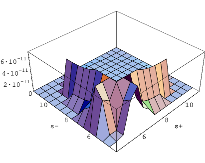
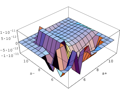
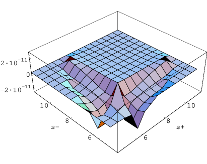
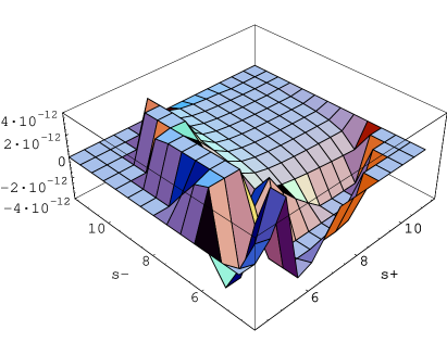
Figure 2: The functions $G_{0}$ (up-left), $G_{c}$ (up-right), $Re\tilde{G}_{s}$ (down-left) and $Im\tilde{G}_{s}$ (down-right) in Eq.(9) using the amplitudes reported in Section 3. The variables $s_{\pm}$ are in $GeV^{2}$.

We now consider the time-dependent decay probabilities (8) and (10), which are given in terms of the functions $G_{0}$, $G_{c}$ and $\tilde{G}_{s}$ in Eq.(9). Using the amplitudes ${\overline{\cal A}}$ derived in Section 3 and the values of the input parameters listed above, we get the functions depicted in fig. 2. On the other hand, the functions obtained by the parameterization of the amplitude using the effective Lagrangian in Section 4 are depicted in fig. 3; the comparison between the two figures shows some agreement between the two methods of extrapolating the polar terms.

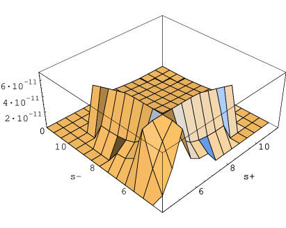
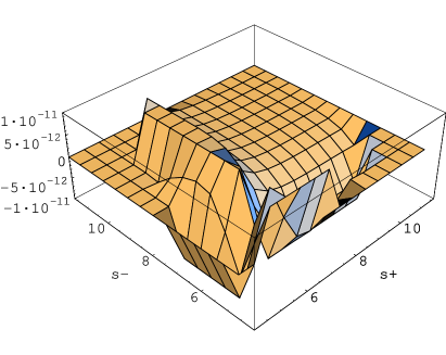
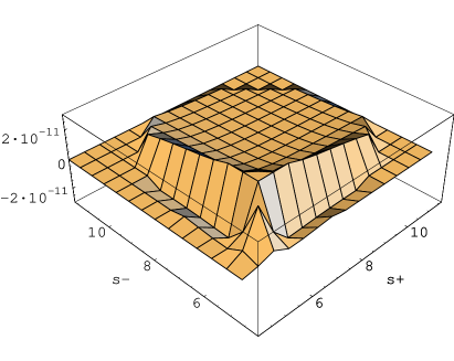
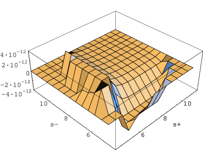
Figure 3: The functions $G_{0}$ (up-left), $G_{c}$ (up-right), $Re\tilde{G}_{s}$ (down-left) and $Im\tilde{G}_{s}$ (down-right) in Eq.(9) using the parameterization of the amplitudes in Section 4.

We observe from both figs. 2 and 3 that the signal arising for the $D^{*}$ and $D_{0}$ poles cannot be easily disentangled; concerning the contribution of the $2^{+}$ pole, the $D^{*+}_{2}$, we find that it is numerically small with respect to the other resonances, due to the small value of the form factor $\tau_{3/2}$ as compared to the constituent quark model value used in Ref. [4].

For an assessment of the relative size of the various contributions to the time-dependent probabilities (8) and (10), we integrate the functions $G_{0}$, $G_{c}$, and $Re\tilde{G}_{s}$ and $Im\tilde{G}_{s}$ over the region bounded by Eqs.(6),(7), with $s_{+}\geq s_{-}$, corresponding to one half of the Dalitz plot. We find, using the functions in fig. 3: $\int G_{0}(s_{+},s_{-})ds_{+}ds_{-}\simeq 7\times 10^{-10}$ GeV⁴, $\int G_{c}(s_{+},s_{-})ds_{+}ds_{-}\simeq-7\times 10^{-11}$ GeV⁴, $\int Re\tilde{G}_{s}(s_{+},s_{-})ds_{+}ds_{-}\simeq 2\times 10^{-10}$ GeV⁴, $\int Im\tilde{G}_{s}(s_{+},s_{-})ds_{+}ds_{-}\simeq-8\times 10^{-11}$ GeV⁴. These numbers may represent an indication on the sensitivity (hence, on the required statistics) of a combined time-dependent and Dalitz plot analysis of the events to the terms $\cos(\Delta mt)$ and $\sin(\Delta mt)$, as well as to $\sin(2\beta)$ and $\cos(2\beta)$. In particular, they suggest that the contribution of $\cos(2\beta)$ to the time-dependent CP asymmetry may be sufficiently large to be identified.

6 The decay $B\to D^{+}D^{-}K_{S}$

The kinematics of this process is quite similar to the case of the Cabibbo suppressed $B\to D^{+}D^{-}\pi^{0}$ transition discussed above. Apart from the change $m_{\pi}\to m_{K}$ which reduces the available phase space, and the replacement of the $D^{*}$ resonance by the $D^{*}_{s}$ one, there are two important differences with respect to the case of the neutral pion in the final state. Indeed, as being induced at the quark level by the $b\to c\bar{c}s$ transition, the amplitude for this channel is both color-allowed and Cabibbo favored by a factor $V_{cs}/V_{cd}$, so that one expects an enhanced rate of events (and, possibly, a better efficiency of the $K_{S}$ reconstruction as compared to the $\pi^{0}$). Moreover, due to the flavour structure, beauty intermediate states (hence the amplitudes ${\overline{\cal A}}_{2,3,9}$ corresponding to fig.1a) are absent, and the same is true for the $D^{*-}_{s}$ resonances in $\bar{B}_{0}$ decays (amplitudes ${\overline{\cal A}}_{5,7}$ in fig.1b). In addition, the $D^{*}_{s2}$ does not contribute in the factorization approximation. Therefore, the resonant structure of the amplitude turns out to be much simpler (although the parameters of the relevant Breit-Wigner forms are still to be measured). On the other hand, due to the significantly larger value of $m_{K}$, the uncertainty implicit in the application of the chiral symmetry approach is expected to be larger for $B\to D^{+}D^{-}K_{S}$. As far as $SU(3)_{F}$ breaking effects are concerned, we partially take them into account by replacing $f_{\pi}\to f_{K}$ ($f_{K}=160$ MeV) in the relevant formulae reported in the previous Sections.

As a result, we obtain for ${\overline{B}^{0}}\to D^{+}D^{-}K_{S}$ the width $\Gamma({\overline{B}^{0}}\to D^{+}D^{-}K_{S})\simeq 4\times 10^{-15}$ GeV, corresponding to the branching fraction ${\cal B}({\overline{B}^{0}}\to D^{+}D^{-}K_{S})\simeq 9\times 10^{-3}$. This result indicates an enhancement of a factor 10 with respect to $B\to D^{+}D^{-}\pi^{0}$, rather than 20 naively represented by $|V_{cs}/V_{cd}|^{2}$, and this is a consequence of the larger value of $m_{K}$ reducing the phase-space, and of the smaller number of intermediate resonances active in this case.

The functions relevant for the time-dependent processes Eqs. (8) and (10) are depicted in fig.4 which shows the expected simpler Dalitz-plot structure, as far as the $s_{+}$ and $s_{-}$ dependence is concerned, with respect to the process (1).

The corresponding integrals over half of the Dalitz plot of such functions turn out to be: $\int G_{0}(s_{+},s_{-})ds_{+}ds_{-}\simeq 5\times 10^{-9}$ GeV⁴, $\int G_{c}(s_{+},s_{-})ds_{+}ds_{-}\simeq-2\times 10^{-9}$ GeV⁴,
$\int Re\tilde{G}_{s}(s_{+},s_{-})ds_{+}ds_{-}\simeq 2\times 10^{-9}$ GeV⁴, $\int Im\tilde{G}_{s}(s_{+},s_{-})ds_{+}ds_{-}\simeq-6\times 10^{-10}$ GeV⁴.

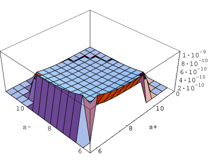
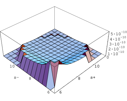
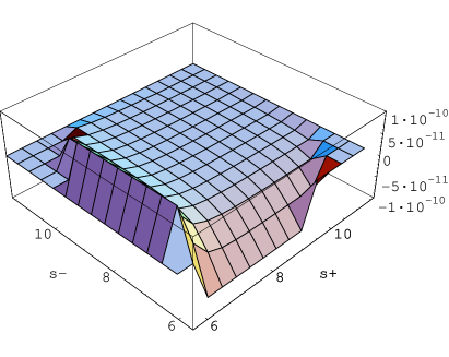
Figure 4: The functions $G_{0}$ (up-left), $G_{c}$ (up-right), $Re\tilde{G}_{s}$ (down-left) and $Im\tilde{G}_{s}$ (down-right) in Eq.(9) for the transition $B\to D^{+}D^{-}K_{S}$.

7 Conclusions

We have analyzed the three-body decays $B\to D^{+}D^{-}\pi^{0}$ and $B\to D^{+}D^{-}K_{S}$ using a resonance model taking into account the constraints of the chiral symmetry on the relevant transition matrix elements. This method introduces a non-resonant, contact term as well as specific behaviour of the Breit-Wigner residue.

The main conclusion of our model can be seen in figs. 2 and 3, which show that the coefficient of $\cos(2\beta)$ in the time-dependent rate, namely $Im\tilde{G}_{s}$, is significantly different from zero over a sufficiently large portion of the Dalitz plot. Therefore, in principle, apart from its specific interest as a test of the chiral expansion in the heavy-quark theory, this channel might be useful to resolve the ambiguity in the determination of the CKM phase $\beta$ ($\beta\to{\pi\over 2}-\beta$). Indeed, once $\sin(2\beta)$ is measured from, e.g., $B\to J/\psi K_{S}$, the required information should be given by a suitable combination according to Eq.(8) of the two Dalitz plot distributions in the lower row of figs.2 or 3.

Qualitatively, our conclusions about the model dependence of the polar representation and the $D^{\pm}$ and $\pi^{0}$ reconstruction efficiency agree with Ref.[4]. From the numerical point of view, the differences with respect to [4] are mainly due to the inclusion of the equal-time commutator and the parameterization of the resonances. Indeed, the starting point of our calculation is the possibility of using the effective chiral lagrangian formalism for heavy mesons, offered by the smallness of the phase space available to the $\pi^{0}$. Another source of difference is the use of a smaller $\tau_{3/2}$ form factor (as resulting from QCD sum rules) which depresses the contribution of $D_{2}^{*}$.

Finally, we emphasize the obtained large branching ratio ${\cal B}(B\to D^{+}D^{-}K_{S})\simeq 9\times 10^{-3}$ which, together with the simpler Dalitz plot structure and the better $K_{S}$ reconstruction efficiency, can make this channel rather appealing for experimental analyses.

Acknowledgments
(R) would like to acknowledge the support of KFUPM . He also thanks ICTP, Trieste, for hospitality during the summer of 1998.

References

• [1] C. Caso et al., (Particle Data Group), Eur. Phys. J. C3, 1 (1998).
• [2] For a recent review see: The BaBar Physics Book, P.F. Harrison and H. R. Quinn. eds., SLAC-R-504 (October 1998).
• [3] A.E. Snyder and H.R. Quinn, Phys. Rev. D48, 2139 (1993).
• [4] J. Charles, A. Le Yaouanc, L. Oliver, O. PΓ¨ne and J.-C. Raynal, Phys. Lett. B425, 375 (1998); 433, 441 (1998) (E).
• [5] A.J. Buras and R. Fleischer, in Heavy Flavours II, A.J. Buras and M. Lindner eds., World Scientific, Singapore, 1998.
• [6] Y. Grossman, and H.R. Quinn, Phys. Rev. D56, 7259 (1997); L. Wolfenstein, Phys. Rev. D57, 6857 (1997) ; A.S. Dighe, I. Dunietz and R. Fleischer, Phys. Lett. B433, 147 (1998).
• [7] A discussion of such effects is reported in Ch. 5 of Ref. [2].
• [8] A.I. Sanda and Z. Xing, Phys. Rev. D56, 6866 (1997).
• [9] For reviews on the Heavy Quark Effective Theory see: H. Georgi, in Proceedings of TASI 91, R.K. Ellis ed., World Scientific, Singapore,1991; B. Grinstein, in High Energy Phenomenology, R. Huerta and M.A. Peres eds., World Scientific, Singapore, 1991; N. Isgur and M. Wise, in Heavy Flavours, A. Buras and M. Lindner eds., World Scientific, Singapore,1992; M. Neubert, Phys. Rep. 245, 259 (1994).
• [10] R.E. Marshak, Riazuddin and C.P. Ryan, Theory of weak interactions in particle physics, Wiley, N.Y., 1969.
• [11] R. Casalbuoni, A. Deandrea, N. Di Bartolomeo, F. Ferruccio, R. Gatto and G. Nardulli, Phys. Rep. 281, 145 (1997).
• [12] A.F. Falk and M. Luke, Phys. Lett. B292, 119 (1992).
• [13] P. Colangelo, A. Deandrea, N. Di Bartolomeo, F. Feruglio, R. Gatto and G. Nardulli, Phys. Lett. B339, 151 (1994); P. Colangelo, F. De Fazio, N. Di Bartolomeo, R. Gatto, G. Nardulli, Phys.Rev. D52, 6422 (1995); P. Colangelo and F. De Fazio, Eur. Phys. J. C4, 503 (1998).
• [14] V.M. Belyaev, V.M. Braun, A. Khodjamirian and R. RΓΌckl, Phys. Rev. D51 6177 (1995); S. Narison and H.G. Dosch, Phys. Lett. B368, 163 (1996).
• [15] D.J. Broadhurst and A.G. Grozin, Phys. Lett. B274, 421 (1992); M. Neubert, Phys. Rev. D45, 2451 (1992).
• [16] Y.B. Dai, C.S. Huang, M.Q. Huang and C. Liu, Phys. Lett. B390, 350 (1997); Y.B. Dai, C.S. Huang and M.Q. Huang, Phys. Rev. D55, 5719 (1997).
• [17] M. Neubert, Phys. Rev. D47, 4063 (1993).
• [18] E. Bagan, P. Ball and P. Gosdzinsky, Phys. Lett. B301, 249 (1993).
• [19] P. Colangelo, F. De Fazio and N. Paver, Phys. Rev. D58, 116005 (1998).
• [20] P. Colangelo, G. Nardulli and N. Paver, Phys. Lett. B293, 207 (1992).
• [21] Other analyses of the universal form factors can be found in Y.B. Dai and M.Q. Huang, hep-ph/9807461; V. Morenas, A. Le Yaouanc, L. Oliver, O. Pene and J.C. Raynal, Phys. Rev. D56, 5668 (1997); D. Ebert and R.N. Faustov, Phys. Lett. B434, 365 (1998); A. Deandrea, N. Di Bartolomeo, R. Gatto, G. Nardulli and A. Polosa, Phys. Rev. D58, 034004 (1998).
• [22] M. Artuso et al., CLEO Collab., CLNS 98/1589, CLEO 98-17, hep-ex/9811027.