Rare Kaon Decays and CP Violation

RARE KAON DECAYS AND CP VIOLATION

© Copyright by Fabrizio Gabbiani 1997

All Rights Reserved

RARE KAON DECAYS AND CP VIOLATION

  John F. Donoghue, Department Head Physics and Astronomy

To the Opera Singer

ABSTRACT

RARE KAON DECAYS AND CP VIOLATION
SEPTEMBER 1997
FABRIZIO GABBIANI
LAUREA IN FISICA, UNIVERSITÀ DEGLI STUDI DI PADOVA
Ph.D., UNIVERSITY OF MASSACHUSETTS AMHERST
Directed by: Professor John F. Donoghue

Rare kaon decays are an important testing ground of the electroweak flavor theory. They can provide new signals of CP-violating phenomena and open a window into physics beyond the Standard Model. The interplay of long-distance QCD effects in strangeness-changing transitions can be analyzed with Chiral Perturbation Theory techniques. Some theoretical predictions obtained within this framework for radiative kaon decays are reviewed, together with the present experimental status. In particular, two rare kaon decays are analyzed: The first decay, $K_{L}\rightarrow\pi^{0}e^{+}e^{-}$, is being searched for as a signal of direct $\Delta S=1$ CP violation. We provide a thorough updating of the analysis of the three components of the decay: 1) Direct CP violation, 2) CP violation through the mass matrix and 3) CP-conserving (two-photon) contributions. First the chiral calculation of the $K_{S}\rightarrow\pi^{0}e^{+}e^{-}$ rate, due to Ecker, Pich and de Rafael, is updated to include recent results on the nonleptonic amplitude. Then we systematically explore the uncertainties in this method. These appear to be so large that they will obscure the direct CP violation unless it is possible to measure the $K_{S}\rightarrow\pi^{0}e^{+}e^{-}$ rate. The CP-conserving amplitude remains somewhat uncertain, but present indications are such that there may be a sizable CP-violating asymmetry in the $e^{+},e^{-}$ energies from the interference of CP-conserving and CP-violating amplitudes and this may potentially be useful in determining whether direct CP violation is present. The second decay, $K_{L}\rightarrow\pi^{0}\gamma e^{+}e^{-}$, which occurs at a higher rate than the nonradiative process $K_{L}\rightarrow\pi^{0}e^{+}e^{-}$, can be a background to CP violation studies using the latter reaction. It also has interest in its own right in the context of Chiral Perturbation Theory, through its relation to the decay $K_{L}\rightarrow\pi^{0}\gamma\gamma$. The leading order chiral loop contribution to $K_{L}\rightarrow\pi^{0}\gamma e^{+}e^{-}$, including the $(q_{e^{+}}+q_{e^{-}})^{2}/m^{2}_{\pi}$ dependence, is completely calculable. We present this result and also include the higher order modifications that are required in the analysis of $K_{L}\rightarrow\pi^{0}\gamma\gamma$.

TABLE OF CONTENTS

toc

LIST OF TABLES

lot

LIST OF FIGURES

lof

Chapter 1 INTRODUCTION

High-precision experiments on rare kaon decays offer the possibility of unraveling new physics beyond the Standard Model. Searching for forbidden flavor-changing processes [1] at the $10^{-10}$ level [$BR(K_{L}\rightarrow\mu e)<3.3\times 10^{-11}$, $BR(K_{L}\rightarrow\pi^{0}\mu e)<3.2\times 10^{-9}$, $BR(K^{+}\rightarrow\pi^{+}\mu e)<2.1\times 10^{-10}$, …], one is actually exploring energy scales above the 10 TeV region. The study of allowed (but highly suppressed) decay modes provides, at the same time, very interesting tests of the Standard Model itself. Electromagnetic-induced nonleptonic weak transitions and higher-order weak processes are a useful tool to improve our understanding of the interplay among electromagnetic, weak and strong interactions. In addition, new signals of CP violation, which would help to elucidate the source of CP-violating phenomena, can be looked for.

In this chapter we shall briefly describe a few relevant rare kaon decays, reserving the rest of this thesis for the processes $K_{L}\rightarrow\pi^{0}\gamma\gamma$, $K_{L}\rightarrow\pi^{0}e^{+}e^{-}$ and $K_{L}\rightarrow\pi^{0}\gamma e^{+}e^{-}$, together with the related decays $K^{+}\rightarrow\pi^{+}\gamma\gamma$ and $K^{+}\rightarrow\pi^{+}e^{+}e^{-}$.

Since the kaon mass is a very low energy scale, the theoretical analysis of nonleptonic kaon decays is highly non-trivial. While the underlying flavor-changing weak transitions among the constituent quarks are associated with the $W$-mass scale, the corresponding hadronic amplitudes are governed by the long-distance behavior of the strong interactions, i.e. the confinement regime of QCD.

The standard short-distance approach to weak transitions makes use of the asymptotic freedom property of QCD to successively integrate out the fields with heavy masses down to scales $\mu<m_{c}$. Using the operator product expansion (OPE) and renormalization-group techniques, one gets an effective $\Delta S=1$ hamiltonian,

$${\cal H}_{\mbox{\rm\scriptsize eff}}^{\Delta S=1}\,=\,{G_{F}\over\sqrt{2}}V_{ud}^{\phantom{*}}V_{us}^{*}\,\sum_{i}C_{i}(\mu)Q_{i}\,+\,\mbox{\rm h.c.},$$ (1.1)

which is a sum of local four-fermion operators $Q_{i}$, constructed with the light degrees of freedom ($u,d,s;e,\mu,\nu_{l}$), modulated by Wilson coefficients $C_{i}(\mu)$ which are functions of the heavy ($W,t,b,c,\tau$) masses. The overall renormalization scale $\mu$ separates the short- ($M>\mu$) and long- ($m<\mu$) distance contributions, which are contained in $C_{i}(\mu)$ and $Q_{i}$, respectively. The physical amplitudes are of course independent of $\mu$; thus, the explicit scale (and scheme) dependence of the Wilson coefficients, should cancel exactly with the corresponding dependence of the $Q_{i}$ matrix elements between on-shell states.

Our knowledge of the $\Delta S=1$ effective hamiltonian has improved considerably in recent years, thanks to the completion of the next-to-leading logarithmic order calculation of the Wilson coefficients [2]. All gluonic corrections of ${\cal O}(\alpha_{s}^{n}t^{n})$ and ${\cal O}(\alpha_{s}^{n+1}t^{n})$ are already known, where $t\equiv\log{(M/m)}$ refers to the logarithm of any ratio of heavy-mass scales ($M,m\geq\mu$). Moreover, the full $m_{t}/M_{W}$ dependence (at lowest order in $\alpha_{s}$) has been taken into account.

Unfortunately, in order to predict the physical amplitudes one is still confronted with the calculation of the hadronic matrix elements of the quark operators. This is a very difficult problem, which so far remains unsolved. We have only been able to obtain rough estimates using different approximations (vacuum saturation, $N_{C}\rightarrow\infty$ limit, QCD low-energy effective action, …) or applying QCD techniques (lattice, QCD sum rules) which suffer from their own technical limitations.

Below the resonance region ($\mu<m_{\rho}$) the strong interaction dynamics can be better understood with global symmetry considerations. We can take advantage of the fact that the pseudoscalar mesons are the lowest energy modes of the hadronic spectrum: They correspond to the octet of Goldstone bosons associated with the dynamical chiral symmetry breaking of QCD, $SU(3)_{L}\otimes SU(3)_{R}\rightarrow SU(3)_{V}$. The low-energy implications of the QCD symmetries can then be worked out through an effective lagrangian containing only the Goldstone modes. The effective Chiral Perturbation Theory [3] (ChPTh) formulation of the Standard Model is an ideal framework to describe kaon decays [4]. This is because in $K$ decays the only physical states that appear are pseudoscalar mesons, photons and leptons, and because the characteristic momenta involved are small compared to the natural scale of chiral symmetry breaking ($\Lambda_{\chi}\sim 1$ GeV).

1.1 $K\rightarrow\pi\nu{\overline{\nu}}$

The decays $K\to\pi\nu\overline{\nu}$ proceed through flavor-changing neutral current effects. These arise in the Standard Model only at second (one-loop) order in the electroweak interaction (Z-penguin and W-box diagrams, Fig. 1) and are additionally GIM suppressed.

The branching fractions are thus very small, at the level of $10^{-10}$, which makes these modes rather challenging to detect. However, $K\to\pi\nu\overline{\nu}$ have long been known to be reliably calculable, in contrast to most other decay modes of interest. A measurement of $K^{+}\to\pi^{+}\nu\overline{\nu}$ and $K_{L}\to\pi^{0}\nu\overline{\nu}$ will therefore be an extremely useful test of flavor physics. Over the recent years important refinements have been added to the theoretical treatment of $K\to\pi\nu\overline{\nu}$. Let us briefly summarize the main aspects of why $K\to\pi\nu\overline{\nu}$ is theoretically so favorable and what recent developments have contributed to emphasize this point.

Figure 1.1: Diagrams inducing the decay $s\rightarrow d\nu{\overline{\nu}}$ in the Standard Model.

a)

First, $K\to\pi\nu\overline{\nu}$ is semileptonic. The relevant hadronic matrix elements, such as $\langle\pi|(\overline{s}d)_{V-A}|K\rangle$, are just matrix elements of a current operator between hadronic states, which are already considerably simpler objects than the matrix elements of four-quark operators encountered in many other observables ($K-\overline{K}$ mixing, $\epsilon^{\prime}/\epsilon$). Moreover, they are related to the matrix element

$$\langle\pi^{0}|(\overline{s}u)_{V-A}|K^{+}\rangle$$ (1.2)

by isospin symmetry. The latter quantity can be extracted from the well measured leading semileptonic decay $K^{+}\to\pi^{0}l\nu$. Although isospin is a fairly good symmetry, it is still broken by the small up-down quark mass difference and by electromagnetic effects. These manifest themselves in differences of the neutral versus charged kaon (pion) masses (affecting phase space), corrections to the isospin limit in the form factors and electromagnetic radiative effects. Marciano and Parsa [5] have analyzed these corrections and found an overall reduction in the branching ratio by $10\%$ for $K^{+}\to\pi^{+}\nu\overline{\nu}$ and $5.6\%$ for $K_{L}\to\pi^{0}\nu\overline{\nu}$.

b)

Long distance contributions are systematically suppressed as ${\cal O}(\Lambda^{2}_{QCD}/$$m^{2}_{c})$ compared to the charm contribution (which is part of the short distance amplitude). This feature is related to the hard ($\sim m^{2}_{c}$) GIM suppression pattern shown by the Z-penguin and W-box diagrams, and the absence of virtual photon amplitudes. Long distance contributions have been examined quantitatively [6] and shown to be numerically negligible (below $\approx 5\%$ of the charm amplitude).

c)

The preceding discussion implies that $K\to\pi\nu\overline{\nu}$ are short distance dominated by top- and charm-loops in general. The relevant short distance QCD effects can be treated in perturbation theory and have been calculated at next-to-leading order [7]. This allowed to substantially reduce (for $K^{+}$) or even practically eliminate ($K_{L}$) the leading order scale ambiguities, which are the dominant uncertainties in the leading order result.

The decay amplitude for $K\rightarrow\pi\nu\overline{\nu}$,

$$\mbox{}\!\!{\cal M}(K\rightarrow\pi\nu\overline{\nu})\,\sim\,\sum_{i=c,t}F(V_{id}^{\phantom{*}}V_{is}^{*};x_{i})\left(\overline{\nu}^{\phantom{l}}_{L}\gamma_{\mu}\nu^{\phantom{l}}_{L}\right)\langle\pi|\overline{s}_{L}\gamma^{\mu}d_{L}|K\rangle\,,\qquad x_{i}\equiv m_{i}^{2}/M_{W}^{2},$$ (1.3)

involves the hadronic matrix element of the $\Delta S=1$ vector current, which (assuming isospin symmetry) can be obtained from $K_{l3}$ decays. In the ChPTh framework, the needed hadronic matrix element is known at ${\cal O}(E^{4})$; this allows one to estimate the relevant isospin-violating corrections reliably [8, 5].

Summing over the three neutrino flavors and expressing the quark-mixing factors through the Wolfenstein parameters [9] $\lambda$, $A$, $\rho$ and $\eta$, one can write the approximate formula [2]:

$$BR(K^{+}\rightarrow\pi^{+}\nu\overline{\nu})\,\approx\,1.93\times 10^{-11}\,A^{4}\,x_{t}^{1.15}\,\left[\eta^{2}+(\rho_{0}-\rho)^{2}\right]\,,\qquad\rho_{0}\approx 1.4\,.$$ (1.4)

The departure of $\rho_{0}$ from unity measures the impact of the charm contribution.

With the presently favored values for the quark-mixing parameters, the branching ratio is predicted to be in the range [2]

$$BR(K^{+}\rightarrow\pi^{+}\nu\overline{\nu})\,=\,(9.1\pm 3.2)\times 10^{-11}\,,$$ (1.5)

to be compared with the present experimental upper bound [10] $BR(K^{+}\rightarrow\pi^{+}\nu\overline{\nu})$ $<$ 2.4$\times 10^{-9}$ (90% CL).

What is actually measured is the transition $K^{+}\rightarrow\pi^{+}+$ nothing; therefore, the experimental search for this process can also be used to set limits on possible exotic decay modes like $K^{+}\rightarrow\pi^{+}X^{0}$, where $X^{0}$ denotes an undetected light Higgs or Goldstone boson (axion, familon, majoron, …).

The CP-violating decay $K_{L}\rightarrow\pi^{0}\nu\overline{\nu}$ has been suggested [11] as a good candidate to look for pure direct CP-violating transitions. The contribution coming from indirect (mass-matrix) CP violation via $K^{0}$-${\overline{K}}^{0}$ mixing is very small [11]: $BR(K_{L}\rightarrow\pi^{0}\nu\overline{\nu})_{\rm MM}$ $\sim$ 5 $\times 10^{-15}$. The decay proceeds almost entirely through direct CP violation, and is completely dominated by short-distance loop diagrams with top quark exchanges [2]:

$$BR(K_{L}\rightarrow\pi^{0}\nu\overline{\nu})\,\approx\,8.07\times 10^{-11}\,A^{4}\,\eta^{2}\,x_{t}^{1.15}\,.$$ (1.6)

The present experimental upper bound [12], $BR(K_{L}\rightarrow\pi^{0}\nu\overline{\nu})<5.8\times 10^{-5}$ (90% CL), is still far away from the expected range [2]

$$BR(K_{L}\rightarrow\pi^{0}\nu\overline{\nu})\,=\,(2.8\pm 1.7)\times 10^{-11}\,.$$ (1.7)

Nevertheless, the experimental prospects to reach the required sensitivity in the near future look rather promising. The clean observation of just a single unambiguous event would indicate the existence of CP-violating $\Delta S=1$ transitions.

In Table 1 we have summarized some of the main features of $K^{+}\to\pi^{+}\nu\overline{\nu}$ and $K_{L}\to\pi^{0}\nu\overline{\nu}$.

Table 1.1: Important properties and results for $K\to\pi\nu\overline{\nu}$.

	$K^{+}\to\pi^{+}\nu\overline{\nu}$	$K_{L}\to\pi^{0}\nu\overline{\nu}$
	CP-conserving	CP-violating
CKM	$V_{td}$	$\mbox{Im}V^{*}_{ts}V^{\phantom{*}}_{td}\sim J_{\rm CP}\sim\eta$
scale uncert. (BR)	$\pm 20\%$ (LO) $\to\pm 5\%$ (NLO)	$\pm 10\%$ (LO) $\to\pm 1\%$ (NLO)
BR (SM)	$(0.9\pm 0.3)\times 10^{-10}$	$(2.8\pm 1.7)\times 10^{-11}$
exp. limit	$<2.4\times 10^{-9}$ BNL 787 [10]	$<5.8\times 10^{-5}$ FNAL 799 [12]

While already $K^{+}\to\pi^{+}\nu\overline{\nu}$ can be reliably calculated, the situation is even better for $K_{L}\to\pi^{0}\nu\overline{\nu}$. The charm sector, in $K^{+}\to\pi^{+}\nu\overline{\nu}$ the dominant source of uncertainty, is completely negligible for $K_{L}\to\pi^{0}\nu\overline{\nu}$ ($0.1\%$ effect on the branching ratio). Long distance contributions ($\;\raisebox{-1.72218pt}{\hbox to0.0pt{$\sim$\hss}}\raisebox{1.72218pt}{$<$}\;0.1\%$) and also the indirect CP violation effect ($\;\raisebox{-1.72218pt}{\hbox to0.0pt{$\sim$\hss}}\raisebox{1.72218pt}{$<$}\;1\%$) are likewise negligible. In summary, the total theoretical uncertainties, from perturbation theory in the top sector and in the isospin breaking corrections, are safely below $2-3\%$ for $BR(K_{L}\to\pi^{0}\nu\overline{\nu})$. This makes this decay mode truly unique and very promising for phenomenological applications. Note that the range given as the Standard Model prediction in Table 1.1 arises from our, at present, limited knowledge of Standard Model parameters (CKM), and not from intrinsic uncertainties in calculating $BR(K_{L}\to\pi^{0}\nu\overline{\nu})$.

With a measurement of $BR(K^{+}\to\pi^{+}\nu\overline{\nu})$ and $BR(K_{L}\to\pi^{0}\nu\overline{\nu})$ available very interesting phenomenological studies could be performed. For instance, $BR(K^{+}\to\pi^{+}\nu\overline{\nu})$ and $BR(K_{L}\to\pi^{0}\nu\overline{\nu})$ together determine the unitarity triangle (Wolfenstein parameters $\rho$ and $\eta$) completely.

The expected accuracy with $\pm 10\%$ branching ratio measurements is comparable to the one that can be achieved by CP violation studies at $B$ factories before the LHC era [13]. The quantity $BR(K_{L}\to\pi^{0}\nu\overline{\nu})$ by itself offers probably the best precision in determining $\mbox{Im}V^{*}_{ts}V_{td}$ or, equivalently, the Jarlskog parameter [14]

$$J_{\rm CP}=\mbox{Im}(V^{*}_{ts}V_{td}^{\phantom{*}}V_{us}^{\phantom{*}}V^{*}_{ud})=\lambda\left(1-\frac{\lambda^{2}}{2}\right)\mbox{Im}\lambda_{t}.$$ (1.8)

The charged mode $K^{+}\to\pi^{+}\nu\overline{\nu}$ is being currently pursued by Brookhaven experiment E787. The latest published result [10] gives an upper limit which is about a factor 25 above the Standard Model range. Several improvements have been implemented since then and the SM sensitivity is expected to be reached in the near future [15]. Recently an experiment has been proposed to measure $K^{+}\to\pi^{+}\nu\overline{\nu}$ at the Fermilab Main Injector [16]. Concerning $K_{L}\to\pi^{0}\nu\overline{\nu}$, a proposal exists at Brookhaven (BNL E926) to measure this decay at the AGS with a sensitivity of ${\cal O}(10^{-12})$ (see [15]). There are furthermore plans to pursue this mode with comparable sensitivity at Fermilab [17] and KEK [18].

1.2 $K_{S}\rightarrow\gamma\gamma$

The symmetry constraints do not allow any direct tree-level $K_{1}^{0}\gamma\gamma$ coupling at ${\cal O}(E^{4})$ ($K^{0}_{1,2}$ refer to the CP-even and CP-odd eigenstates, respectively). This decay proceeds then through a loop of charged pions and kaons as shown in Fig. 2.

Figure 1.2: Feynman diagrams for $K^{0}_{1}\rightarrow\gamma\gamma$.

Since there are no possible counter-terms to renormalize divergences, the one-loop amplitude is necessarily finite. Although each of the four diagrams in Fig. 2 is quadratically divergent, these divergences cancel in the sum. The resulting prediction [19], $BR(K_{S}\rightarrow\gamma\gamma)=2.0\times 10^{-6}$, is in very good agreement with the experimental measurement [20]:

$$BR(K_{S}\rightarrow\gamma\gamma)\,=\,(2.4\pm 0.9)\times 10^{-6}\,.$$ (1.9)

1.3 $K_{L,S}\rightarrow\mu^{+}\mu^{-}$

There are well-known short-distance contributions [2] (electroweak penguins and box diagrams) to the decay $K_{L}\rightarrow\mu^{+}\mu^{-}$. This part of the amplitude is sensitive to the Wolfenstein parameter $\rho$. However, this transition is dominated by long-distance physics. The main contribution proceeds through a two-photon intermediate state: $K_{2}^{0}\rightarrow\gamma^{*}\gamma^{*}\rightarrow\mu^{+}\mu^{-}$. Contrary to $K_{1}^{0}\rightarrow\gamma\gamma$, the prediction for the $K_{2}^{0}\rightarrow\gamma\gamma$ decay is very uncertain, because the first non-zero contribution occurs at ${\cal O}(E^{6})$. That makes very difficult any attempt to predict the $K_{L}\rightarrow\mu^{+}\mu^{-}$ amplitude.

The long distance amplitude consists of a dispersive ($A_{\rm dis}$) and an absorptive contribution ($A_{\rm abs}$). The branching fraction can thus be written

$$BR(K_{L}\to\mu^{+}\mu^{-})=|A_{\rm SD}+A_{\rm dis}|^{2}+|A_{\rm abs}|^{2}.$$ (1.10)

Using the well-known unitarity bound

$${{\Gamma(K_{L}\to\mu^{+}\mu^{-})}\over{\Gamma(K_{L}\to\gamma\gamma)}}\geq{{\alpha^{2}m^{2}_{\mu}}\over{2\beta m^{2}_{K}}}\left(\log{{1+\beta}\over{1-\beta}}\right)^{2},\qquad\beta=\sqrt{1-4m^{2}_{\mu}/m^{2}_{K}},$$ (1.11)

associated with the $\gamma\gamma$ intermediate state, and knowing $BR(K_{L}\to\gamma\gamma)$ it is possible to extract $|A_{\rm abs}|^{2}=(6.8\pm 0.3)\times 10^{-9}$ [21]. $A_{\rm dis}$ on the other hand cannot be calculated accurately at present and the estimates are strongly model dependent [22]. This is rather unfortunate, in particular since $BR(K_{L}\to\mu^{+}\mu^{-})$, unlike most other rare decays, has already been measured, and this with very good precision:

$$BR(K_{L}\to\mu^{+}\mu^{-})=\left\{\begin{array}[]{ll}(6.9\pm 0.4)\times 10^{-9},&\mbox{BNL 791 \cite[cite]{[\@@bibref{}{HEIN}{}{}]}},\\ (7.9\pm 0.7)\times 10^{-9},&\mbox{KEK 137 \cite[cite]{[\@@bibref{}{AKA}{}{}]}}.\end{array}\right.$$ (1.12)

For comparison we note that $BR(K_{L}\to\mu^{+}\mu^{-})_{\rm SD}=(1.3\pm 0.6)\times 10^{-9}$ is the expected branching ratio in the Standard Model based on the short-distance contribution alone. Due to the fact that $A_{\rm dis}$ is largely unknown, $K_{L}\to\mu^{+}\mu^{-}$ is at present not a very useful constraint on CKM parameters. Some improvement might be expected from measuring the decay $K_{L}\rightarrow\mu^{+}\mu^{-}e^{+}e^{-}$, which could lead to a better understanding of the $K_{L}\rightarrow\gamma^{*}\gamma^{*}$ vertex. First results obtained at Fermilab (E799) give $BR(K_{L}\rightarrow\mu^{+}\mu^{-}e^{+}e^{-})$ = $(2.9^{+6.7}_{-2.4})\times 10^{-9}$.

The situation is completely different for the $K_{S}$ decay. A straightforward chiral analysis [25] shows that, at lowest order in momenta, the only allowed tree-level $K^{0}\mu^{+}\mu^{-}$ coupling corresponds to the CP-odd state $K_{2}^{0}$. Therefore, the $K_{1}^{0}\rightarrow\mu^{+}\mu^{-}$ transition can only be generated by a finite non-local two-loop contribution, illustrated in Fig. 3.

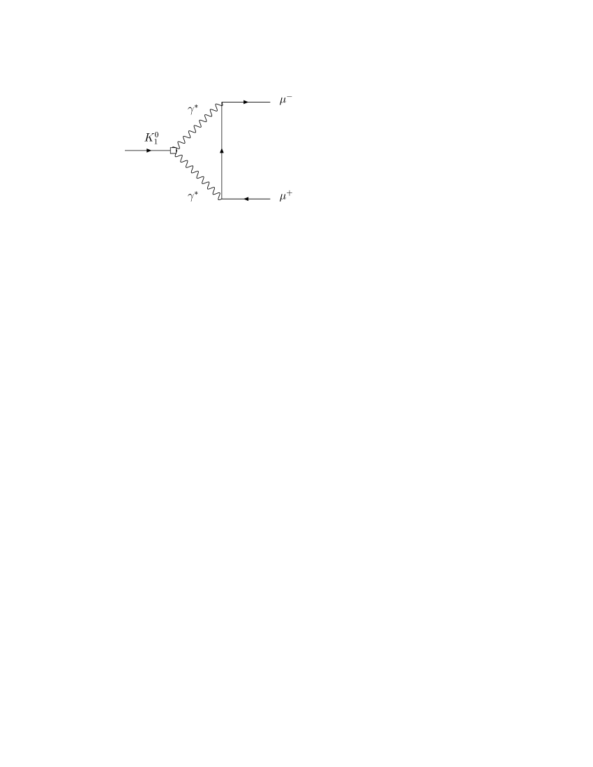
Figure 1.3: Feynman diagram for the decay $K^{0}_{1}\rightarrow\mu^{+}\mu^{-}$. The $K^{0}_{1}\gamma^{*}\gamma^{*}$ vertex is generated through the one-loop diagrams shown in Fig. 2.

The explicit calculation [25] gives:

$${\Gamma(K_{S}\rightarrow\mu^{+}\mu^{-})\over\Gamma(K_{S}\rightarrow\gamma\gamma)}=2\times 10^{-6},\qquad\qquad{\Gamma(K_{S}\rightarrow e^{+}e^{-})\over\Gamma(K_{S}\rightarrow\gamma\gamma)}=8\times 10^{-9},$$ (1.13)

well below the present (90% CL) experimental upper limits [26]: $BR(K_{S}\rightarrow\mu^{+}\mu^{-})$ $<$ $3.2\times 10^{-7}$, $BR(K_{S}\rightarrow e^{+}e^{-})$ $<$ $2.8\times 10^{-6}$. Although, in view of the smallness of the predicted ratios, this calculation seems quite academic, it has important implications for CP-violation studies.

The longitudinal muon polarization ${\cal P}_{L}$ in the decay $K_{L}\rightarrow\mu^{+}\mu^{-}$ is an interesting measure of CP violation. As for every CP-violating observable in the neutral kaon system, there are in general two different kinds of contributions to ${\cal P}_{L}$: Indirect mass-matrix CP violation through the small $K_{1}^{0}$ admixture of the $K_{L}$ ($\epsilon$ effect), and direct CP violation in the $K_{2}^{0}\rightarrow\mu^{+}\mu^{-}$ decay amplitude.

In the Standard Model, the direct CP-violating amplitude is induced by Higgs exchange with an effective one-loop flavor-changing $\overline{s}dH$ coupling [27]. The present lower bound on the Higgs mass, $M_{H}>66$ GeV (95% CL), implies a conservative upper limit $|{\cal P}_{L,\mbox{\rm\scriptsize dir}}|<10^{-4}$. Much larger values, ${\cal P}_{L}\sim{\cal O}(10^{-2})$, appear quite naturally in various extensions of the Standard Model [28]. It is worth emphasizing that ${\cal P}_{L}$ is especially sensitive to the presence of light scalars with CP-violating Yukawa couplings. Thus, ${\cal P}_{L}$ seems to be a good signature to look for new physics beyond the Standard Model; for this to be the case, however, it is very important to have a good quantitative understanding of the Standard Model prediction to allow us to infer, from a measurement of ${\cal P}_{L}$, the existence of a new CP-violation mechanism.

The chiral calculation of the $K_{1}^{0}\rightarrow\mu^{+}\mu^{-}$ amplitude allows us to make a reliable estimate of the contribution to ${\cal P}_{L}$ due to $K^{0}$-$\overline{K}^{0}$ mixing [25]:

$$1.9\,<\,|{\cal P}_{L,{\rm MM}}|\times 10^{3}\Biggl{[}{2\times 10^{-6}\over BR(K_{S}\rightarrow\gamma\gamma)}\Biggr{]}^{1/2}\,<2.5\,.$$ (1.14)

Taking into account the present experimental errors in $BR(K_{S}\rightarrow\gamma\gamma)$ and the inherent theoretical uncertainties due to uncalculated higher-order corrections, one can conclude that experimental indications for $|{\cal P}_{L}|>5\times 10^{-3}$ would constitute clear evidence for additional mechanisms of CP violation beyond the Standard Model.

1.4 $K^{+}\to\pi^{+}\mu^{+}\mu^{-}$

The rare decay $K^{+}\to\pi^{+}\mu^{+}\mu^{-}$ has recently been measured at Brookhaven (BNL 787) with a branching ratio [29]

$$BR(K^{+}\to\pi^{+}\mu^{+}\mu^{-})=(5.0\pm 0.4\pm 0.6)\times 10^{-8}.$$ (1.15)

This compares well with the estimate from ChPTh $BR(K^{+}\to\pi^{+}\mu^{+}\mu^{-})$ = $(6.2^{+0.8}_{-0.6})$ $\times$ $10^{-8}$ [30]. The branching ratio is completely determined by the long-distance contribution arising from the one-photon exchange amplitude. A short-distance amplitude from Z-penguin and W-box diagrams also exists, but is smaller than the long-distance part by three orders of magnitude and does therefore not play any role in the total rate. However, while the muon pair couples via a vector current $(\overline{\mu}\mu)^{\phantom{l}}_{V}$ in the photon amplitude, the electroweak short-distance mechanism also contains an axial vector piece $(\overline{\mu}\mu)_{A}$. The interference term between these contributions is odd under parity and gives rise to a parity-violating longitudinal $\mu^{+}$ polarization, which can be observed as an asymmetry $\Delta_{LR}=(\Gamma_{R}-\Gamma_{L})/(\Gamma_{R}+\Gamma_{L})$ [31, 32]. $\Gamma_{R(L)}$ denotes the rate of producing a right- (left-) handed $\mu^{+}$ in $K^{+}\to\pi^{+}\mu^{+}\mu^{-}$ decay. The effect occurs for a $\mu^{-}$ instead of $\mu^{+}$ as well, but the polarization measurement is much harder in this case.

$\Delta_{LR}$ is sensitive to the Wolfenstein parameter $\rho$. It is a cleaner observable than $K_{L}\to\mu^{+}\mu^{-}$, although some contamination through long-distance contributions cannot be excluded [32]. At any rate, $\Delta_{LR}$ will be an interesting observable to study if a sensitive polarization measurement becomes feasible. The Standard Model expectation is typically around $\Delta_{LR}\sim 0.5\%$.

1.5 Summary

The field of rare kaon decays raises a broad range of interesting topics, ranging from ChPTh, over Standard-Model flavordynamics to exotic phenomena, thereby covering scales from $\Lambda_{QCD}$ to the weak scale ($M_{W}$, $m_{t}$) and beyond to maybe several hundred TeV’s. In the present chapter we have focused on the flavor physics of the Standard Model and those processes that can be used to test it. Several promising examples of short-distance sensitive decay modes exist, whose experimental study will provide important clues on flavordynamics. On the theoretical side, progress has been achieved over recent years in the calculation of effective Hamiltonians, which by now include the complete NLO QCD effects in essentially all cases of practical interest.

The decay $K_{L}\to\mu^{+}\mu^{-}$ is already measured quite accurately; unfortunately a quantitative use of this result for the determination of CKM parameters is strongly limited by large hadronic uncertainties.

The situation looks very bright for $K\to\pi\nu\overline{\nu}$. The charged mode is experimentally already close and its very clean status promises useful results on $V_{td}$. Finally the decay $K_{L}\to\pi^{0}\nu\overline{\nu}$ is a particular highlight in this field. It could serve for instance as the ideal measure of the Jarlskog parameter $J_{\rm CP}$. Measuring the branching ratio is a real experimental challenge.

It is to be expected that rare kaon decay phenomena will in the future continue to contribute substantially to our understanding of the fundamental interactions.

Chapter 2 THEORETICAL FRAMEWORK

2.1 Motivation

There are three rare decay modes of the long-lived kaon which have interrelated theoretical issues: $K_{L}\rightarrow\pi^{0}\gamma\gamma$, $K_{L}\rightarrow\pi^{0}e^{+}e^{-}$ and $K_{L}\rightarrow\pi^{0}\gamma e^{+}e^{-}$. The first two have been extensively studied; the latter has not been previously calculated. It is the purpose of this thesis to provide a calculation of the latter two processes and describe how they are related to the phenomenology of the first one.

There is a curious and important inverted hierarchy of these decay modes. The rate for the radiative decay $K_{L}\rightarrow\pi^{0}\gamma e^{+}e^{-}$ is a power of $\alpha$ larger than the nonradiative transition $K_{L}\rightarrow\pi^{0}e^{+}e^{-}$. This is because the $K_{L}\rightarrow\pi^{0}e^{+}e^{-}$ transition occurs only through a two-photon intermediate state, or alternatively through a one-photon exchange combined with CP violation (which numerically appears to be roughly of the same size as the two-photon contribution) [33]. The $K_{L}\rightarrow\pi^{0}e^{+}e^{-}$ rate is then of order $\alpha^{4}$. However, in $K_{L}\rightarrow\pi^{0}\gamma e^{+}e^{-}$ we need only a one-photon exchange to the $e^{+}e^{-}$, leading to a rate of order $\alpha^{3}$. Our attention was first called to this inverted hierarchy by an observation that there are infrared divergences in a detailed study of the $K_{L}\rightarrow\pi^{0}e^{+}e^{-}$ two-photon effect [33] which need to be canceled by the one-loop corrections to the radiative mode $K_{L}\rightarrow\pi^{0}\gamma e^{+}e^{-}$ through the contributions of the soft radiative photons. This implies that the theoretical and experimental analyses of $K_{L}\rightarrow\pi^{0}e^{+}e^{-}$ and $K_{L}\rightarrow\gamma\pi^{0}e^{+}e^{-}$ are tied together. The soft and collinear photon regions of $K_{L}\rightarrow\gamma\pi^{0}e^{+}e^{-}$ form potential backgrounds to the studies of CP violation in the $K_{L}\rightarrow\pi^{0}e^{+}e^{-}$ mode.

The $K_{L}\rightarrow\pi^{0}\gamma e^{+}e^{-}$ mode also has an interest of its own. In recent years there have been important phenomenological studies of $K_{L}\rightarrow\pi^{0}\gamma\gamma$ in connection with ChPTh. This decay is calculable at one-loop (i.e., order E⁴) ChPTh with no free parameters, yielding a very distinctive spectrum and a definite rate [34, 35]. Surprisingly, when the experiment was performed the spectrum was confirmed while the measured rate was more than a factor of 2 larger than predicted. The way out of this problem appears to have been provided by Cohen, Ecker and Pich (CEP) [36]. By adding an adjustable new effect at order E⁶, as well as including known corrections to the $K_{L}\rightarrow\pi\pi\pi$ vertex, they found that the predicted rate can be increased dramatically without modifying the shape of the spectrum much. This is also a surprising result, yet as far as we know it is the unique solution to the experimental puzzle. The ingredients of the mode studied in this thesis, $K_{L}\rightarrow\pi^{0}\gamma e^{+}e^{-}$, are the same as for $K_{L}\rightarrow\pi^{0}\gamma\gamma$, except that one of the photons is off shell. Within the framework of the CEP calculation, the ingredients enter with different relative weights for off-shell photons. This will allow us to test the consistency of the theoretical resolution proposed for $K_{L}\rightarrow\pi^{0}\gamma\gamma$.

One of the goals of the next generation of rare kaon decay experiments is to attempt to observe CP violation in the decay $K_{L}\rightarrow\pi^{0}e^{+}e^{-}$. This reaction is special because we expect that direct CP violation (as opposed to the “mass matrix” CP violation already observed in the parameter $\epsilon$) may be the dominant component of the amplitude. This is in contrast with $K_{L}\rightarrow\pi\pi$, where the direct effect is at most a few parts in a thousand of $\epsilon$. Direct CP violation distinguishes the Standard Model from “superweak”-type models [37]. Moreover, the magnitude of the direct CP violation for this reaction is a precise prediction of the Standard Model, with very little hadronic uncertainty. In this thesis, we will update the analysis of the reaction $K_{L}\rightarrow\pi^{0}e^{+}e^{-}$, attempting to understand if we can be certain that an experimental measurement is in fact a signal of direct CP violation.

One difficulty is that there are three possible components to the decay amplitude: 1) A CP-conserving process which proceeds through two-photon exchanges, 2) a mass matrix CP-violating effect proportional to the known parameter $\epsilon$, and 3) the direct $\Delta S=1$ CP-violating effect that we would like to observe. The existence of the first of these shows that simply observing the total decay rate is not sufficient to unambiguously indicate the existence of CP violation. We need to either observe a truly CP-odd decay asymmetry, or else be confident on the basis of a theoretical calculation that the CP-conserving effect is safely smaller than the experimental signal. Unfortunately, the predictions in the literature for each of the components listed above exhibits a range of values, including some estimates where all three are similar in magnitude. However, the quality of the theoretical treatment can improve with time, effort and further experimental input. We will try to assess the present and future uncertainties in the theoretical analysis.

There remain significant experimental difficulties before it is possible to mount a search sensitive to a branching ratio of a few times $10^{-12}$. We will assume that such a sensitivity is reached. At the same time, it is reasonable to assume that we will have improved experimental information on the related rate $K_{L}\rightarrow\pi^{0}\gamma\gamma$, and that theoretical methods have provided a consistent phenomenology of this reaction. The CKM parameters will be somewhat more fully constrained in the future, but hadronic matrix element uncertainties will prevent a precise determination of the parameters relevant for CP violation, at least until B meson CP violation has been extensively explored. With these expectations as our framework, will we be able to prove that the future experimental observation indicates the presence of direct CP violation?

Our analysis shows that one will not be able to prove the existence of direct CP violation from the branching ratio for $K_{L}\rightarrow\pi^{0}e^{+}e^{-}$ unless the decay rate for the related decay $K_{S}\rightarrow\pi^{0}e^{+}e^{-}$ is also observed experimentally. This is yet more difficult than measuring the $K_{L}$ decay, and poses a problem for the program of finding direct CP violation. It is possible but not certain, that the electron charge asymmetry can resolve this issue and, when combined with the rate, signal direct CP violation.

2.2 Overview of the Analysis

There is an extensive analysis associated with each of the three components of the decay amplitude for $K_{L}\rightarrow\pi^{0}e^{+}e^{-}$ that were listed in the introduction, but only one work has appeared so far to treat the decay $K_{L}\rightarrow\pi^{0}\gamma e^{+}e^{-}$ [38]. We will devote separate chapters of this thesis to each of these major issues. The purpose of the present chapter is to highlight the main issues that are to be discussed more fully later, and to indicate how they fit together in an overall description of the decay processes.

For the first process, the direct CP component is, in a way, the simplest. The uncertainties are only in the basic parameters of the Standard Model, i.e., the mass of the top quark and the CKM parameters. The relevant hadronic matrix element is reliably known. Unfortunately the extraction of CKM elements has significant uncertainties, so that only a range of possible values can be given. This range corresponds to $K_{L}\rightarrow\pi^{0}e^{+}e^{-}$ branching ratios of a few times $10^{-12}$. We discuss this range in chapter 3.

The contribution of mass-matrix CP violation is more uncertain. The rate due to this source is given by the parameter $\epsilon$ times the rate for $K_{S}\rightarrow\pi^{0}e^{+}e^{-}$, so that the issue is the prediction of the CP-conserving $K_{S}$ partial rate. Here the primary tool is ChPTh, with the pioneering treatment given by Ecker, Pich and de Rafael (EPR) [34, 35]. In chapter 4, we update their analysis, under essentially the same assumptions. The main new ingredient is the inclusion of the results of the one loop analysis of nonleptonic decays, which decreases the overall strength of the weak $K\rightarrow\pi$ transition. This yields a change in the weak counterterms and a decrease of the rate. However, more important is an assessment of the uncertainties of such a calculation, which we describe in chapter 5. Any such calculation has a range of uncertainties, most of which we are able to estimate based on past experience with chiral calculations. We systematically discuss these. Unfortunately we find that one issue in particular has a devastating sensitivity on this mode. In their analysis, EPR made an assumption that lies outside of ChPTh, that a certain weak counterterm satisfies $w_{2}=4L_{9}$ where $L_{9}$ is a known coefficient in the QCD effective chiral lagrangian. This assumption has no rigor, and the decay rate is very sensitive to the deviation $w_{2}-4L_{9}$. For any reasonable value of direct CP violation, there is an equally reasonable value of $w_{2}$ that can reproduce the corresponding $K_{L}\rightarrow\pi^{0}e^{+}e^{-}$ decay rate. Given a measurement, we will then be intrinsically unable to decide if it is evidence of a nonzero value of direct CP violation or merely measures a value for $w_{2}$. It is this what shows a need to measure the rate $K_{S}\rightarrow\pi^{0}e^{+}e^{-}$.

The third component is the CP-conserving amplitude that proceeds through the two-photon intermediate state $K_{L}\rightarrow\pi^{0}\gamma\gamma,\gamma\gamma\rightarrow e^{+}e^{-}$, described in chapter 6. Here we must first understand the process $K_{L}\rightarrow\pi^{0}\gamma\gamma$. This has been calculated in ChPTh at one loop order and has been measured experimentally. While the shape agrees with the chiral calculation, the theoretical rate misses by a factor of three. This has prompted some reanalyses of the theory of $K_{L}\rightarrow\pi^{0}\gamma\gamma$, which we will take account of. However, the field has not reached a satisfactory conclusion on this mode, and it is clear that in the future the experimental and phenomenological status of this reaction will undoubtedly improve. We study how possible resolutions of these analyses will influence the $K_{L}\rightarrow\pi^{0}\gamma\gamma$ decay rate. Ultimately this component should be satisfactorily understood.

The ultimate problem is then our inability to distinguish, in a measurement of the $K_{L}\rightarrow\pi^{0}e^{+}e^{-}$ decay rate, the direct CP violation from the mass matrix effect. It is possible that the electron energy asymmetry may allow us to make this separation. The electron asymmetry comes from the interference of the CP-conserving two-photon process (even under the interchange of $e^{+}e^{-}$) and the CP-violating one-photon process (odd under the $e^{+}e^{-}$ interchange). For many values of the presently favored parameter range, this asymmetry is very large i.e., of order 50%. In this case its measurement is not far more difficult than a good measurement of the rate. If we in fact are able to reach an understanding of the two-photon process, through future phenomenology and experiments on $K_{L}\rightarrow\pi^{0}\gamma\gamma$, then the asymmetry depends most critically on the CP-violating amplitude. If there is no direct CP violation, there is then a correlation between the $K_{L}\rightarrow\pi^{0}e^{+}e^{-}$ decay rate and the electron asymmetry, parameterized by the unknown coefficient $w_{2}$. As we detail in chapter 7, the presence of direct CP violation would upset this correlation, and in many cases would lead to a drastically different relative size of the asymmetry vs. decay rate, often even changing the sign of the asymmetry. Thus the asymmetry may be used to signal direct CP violation. Unfortunately this method is not foolproof. There exist combinations of values of $w_{2}$ and CKM angles for which the distinction between direct and mass matrix CP violation is not so great. In this case the analysis will be muddied by the inherent uncertainties in the theory. In chapter 7 we also explore the use of $K_{L}-K_{S}$ interference to sort out the direct CP violating amplitude. We outline the computation for the $\cal{O}$(E⁴) ChPTh contributions to the process $K_{L}\rightarrow\pi^{0}\gamma e^{+}e^{-}$ in chapter 8, and then we extend it to $\cal{O}$(E⁶) in chapter 9. Finally, we recapitulate all our conclusions in chapter 10.

Chapter 3 DIRECT CP VIOLATION

Direct $\Delta S=1$ CP violation is manifested in the “penguin” reactions pictured in Fig. 4. The QCD short distance corrections to this mode have been thoroughly analyzed to next-to-leading order by Buras et al. [39] (see also Ciuchini et al. [40]), and we will use their results. The primary weak operator responsible for the transition has the form

$${\cal H}^{\Delta S=1}_{W}={G_{F}\over\sqrt{2}}\left[C_{7V}(\mu)Q_{7V}+C_{7A}Q_{7A}\right],$$ (3.1)

where

$$Q_{7V} = (\overline{s}d)_{V-A}(\overline{e}e)_{V},$$

$$Q_{7A} = (\overline{s}d)_{V-A}(\overline{e}e)_{A}.$$ (3.2)

The dominant contribution to the imaginary part of the coefficient $C_{7i}$ comes from the top quark, so that this is truly a short distance process. The coefficients have a CP-violating component

$${\rm Im}\;C_{7i}=-{\rm Im}\left({V^{\phantom{*}}_{td}V^{*}_{ts}\over V^{\phantom{*}}_{ud}V^{*}_{us}}\right)y^{\phantom{\dagger}}_{7i},$$ (3.3)

with the results of Ref. [39] yielding

$${y_{7V}\over\alpha}=0.743,\qquad{y_{7A}\over\alpha}=-0.736,\qquad m_{t}=175,$$ (3.4)

with very little dependence on $\Lambda_{\overline{MS}}$ (the above is for $\Lambda_{\overline{MS}}$ = 0.3 GeV) and a negligible dependence on the low energy scale $\mu$.

Figure 3.1: “Penguin” diagram inducing $\Delta$S = 1 CP violation.

The matrix element involved is well known via isospin symmetry from the charged current kaon decay, i.e.,

$$\langle\pi^{0}(p^{\phantom{l}}_{\pi})|\overline{d}\gamma_{\mu}s|K^{0}(p^{\phantom{l}}_{K})\rangle={f_{+}(q^{2})\over\sqrt{2}}(p^{\phantom{l}}_{K}+p^{\phantom{l}}_{\pi})_{\mu}+{f_{-}(q^{2})\over\sqrt{2}}(p^{\phantom{l}}_{K}-p^{\phantom{l}}_{\pi})_{\mu},$$ (3.5)

with

$$f_{+}(q^{2}) = 1+\lambda q^{2},$$

$$\lambda = (0.65\pm 0.005)\;{\rm fm}^{2}.$$ (3.6)

The form factor $f_{-}$ does not contribute significantly to the decay because its effect is proportional to $m_{e}$. The decay rate is

$$BR(K_{L}\rightarrow\pi^{0}e^{+}e^{-})_{\rm dir}=4.16({\rm Im}\lambda_{t})^{2}(y^{2}_{7A}+y^{2}_{7V}),$$

$${\rm Im}\lambda_{t}={\rm Im}V^{\phantom{*}}_{td}V^{*}_{ts}=|V^{\phantom{*}}_{ub}||V^{\phantom{*}}_{cb}|\sin\delta=A^{2}\lambda^{5}\eta,$$ (3.7)

where $V^{\phantom{*}}_{td}=|V^{\phantom{*}}_{ub}|\sin\delta$, and $A,\lambda,\eta$ refers to the Wolfenstein parametrization of the CKM matrix [9]. This results in

$$BR(K_{L}\rightarrow\pi^{0}e^{+}e^{-})_{\rm dir}=2.75\times 10^{-12}\times\left({{\rm Im}\lambda_{t}\over 10^{-4}}\right)^{2}\;{\rm for}\;m_{t}=175\;{\rm GeV}.\\ \phantom{l}$$

The dependence on the top quark mass will of course be removed by a convincing precise measurement of $m_{t}$.

The CKM parameter $V_{cb}$ has the most favored values (including the recent CLEO data) [41]

$$V^{\phantom{*}}_{cb}=\left\{\begin{array}[]{ll}0.0375\pm 0.0015\pm 0.0012&{\rm HQET}\quad\cite[cite]{[\@@bibref{}{LK}{}{}]},\\ 0.036\pm 0.002\pm 0.003&B\rightarrow D^{\ast}\ell\nu\;{\rm models},\\ 0.039\pm 0.001\pm 0.004&B\rightarrow X\ell\nu.\end{array}\right.$$ (3.8)

The element $V^{\phantom{*}}_{ub}$ is measured by the inclusive decay $B\rightarrow X_{u}e\nu$ in the electron endpoint region. The two inclusive calculations available yield

$${V^{\phantom{*}}_{ub}\over V^{\phantom{*}}_{cb}}=\left\{\begin{array}[]{ll}0.082\pm 0.006&\left[{\rm ACCMM}\right]\quad\cite[cite]{[\@@bibref{}{ACCMM}{}{}]},\\ 0.074\pm 0.007&\left[{\rm RDB}\right]\quad\cite[cite]{[\@@bibref{}{RDB}{}{}]}.\end{array}\right.$$ (3.9)

Models that calculate a set of exclusive decays ($B\rightarrow Me\nu$) can only be used to provide an upper bound on $V^{\phantom{*}}_{ub}$ since there are many final states (such as $B\rightarrow\pi\pi e\nu$ with $\pi\pi$ nonresonant) that are not calculated. These limits are

$${V^{\phantom{*}}_{ub}\over V^{\phantom{*}}_{cb}}\leq\left\{\begin{array}[]{ll}0.12&[{\rm ISGW}]\quad\cite[cite]{[\@@bibref{}{ISGW}{}{}]},\\ 0.087&[{\rm BSW}]\quad\cite[cite]{[\@@bibref{}{WSB}{}{}]},\\ 0.067&[{\rm KS}]\quad\cite[cite]{[\@@bibref{}{KS}{}{}]}.\end{array}\right.$$ (3.10)

We will use the former measurements to estimate

$$\left|{V^{\phantom{*}}_{ub}\over V^{\phantom{*}}_{cb}}\right|=0.078\pm 0.007\pm 0.010,$$ (3.11)

with the first uncertainty experimental and the second theoretical. In the Wolfenstein parametrization of the CKM matrix, the values of $V^{\phantom{*}}_{cb}$ and $V^{\phantom{*}}_{ub}$ imply

$$A = 0.74\pm 0.06,$$

$$\sqrt{\rho^{2}+\eta^{2}} = 0.355\pm 0.056.$$ (3.12)

Without any further analysis, these measurements imply an upper bound on ${\rm Im}\lambda_{t}$:

$${\rm Im}\lambda_{t} = |V^{\phantom{*}}_{ub}||V^{\phantom{*}}_{cb}|\sin\delta$$ (3.13)

$$\leq (1.0\pm 0.3)\times 10^{-4}\sin\delta.$$

A lower bound on this parameter can be found by consideration of the analysis of $\epsilon$. In the Wolfenstein parametrizations one has the approximate form

$$|\epsilon|=(3.4\times 10^{-3})A^{2}\eta B_{K}\left[1+1.3A^{2}(1-\rho)\left({m_{t}\over m_{W}}\right)^{1.6}\right],$$ (3.14)

where $B_{K}$ parametrizes the hadronic matrix element and is estimated to be in the range $0.33\leq B_{K}\leq 1$. Using $(1-\rho)<1.4$ and $B_{K}<1$ one finds for $m_{t}$ = 175 GeV

$$A^{2}\eta\geq 0.13,$$ (3.15)

so that

$${\rm Im}\lambda_{t}=A^{2}\lambda^{5}\eta\geq 6.8\times 10^{-5}.$$ (3.16)

This brackets the range

$$0.68\times 10^{-4}\leq{\rm Im}\lambda_{t}\leq 1.3\times 10^{-4}.$$ (3.17)

Note that ${\rm Im}\lambda_{t}$ is positive. These constraints yield a decay rate from direct CP violation of magnitude

$$1.25\times 10^{-12}\leq BR(K_{L}\rightarrow\pi^{0}e^{+}e^{-})_{\rm dir}\leq 4.6\times 10^{-12}\;{\rm for}\;m_{t}=175.\\ \phantom{l}$$

Alternately, the “best” values

$${\rm Im}\lambda_{t}=1.0\times 10^{-4},\qquad m_{t}=175\;{\rm GeV},$$ (3.18)

which we will take as our standard reference values, lead to a rate

$$BR(K_{L}\rightarrow\pi^{0}e^{+}e^{-})_{\rm dir}=2.32\times 10^{-12}.$$ (3.19)

A more detailed analysis including a correlation between $\rho$ and $\eta$ inherent in Eq. 3.14, as well as the use of $B^{0}_{d}\overline{B}^{0}_{d}$ mixing (which constrains $A\sqrt{(\rho-1)^{2}+\eta^{2}}$ as a function of $f_{B}$) narrows the range only slightly because hadronic uncertainties dominate.

Chapter 4 REVISING THE EPR ANALYSIS

In this chapter, we review the formalism for analyzing mass matrix CP violation, first set forth by Ecker, Pich, de Rafael (EPR) [34, 35]. This amounts to the prediction of the decay rate for $K_{S}\rightarrow\pi^{0}e^{+}e^{-}$, since the mass matrix effect is defined by

$$A(K_{L}\rightarrow\pi^{0}e^{+}e^{-})|_{\rm MM} \equiv \epsilon A(K_{S}\rightarrow\pi^{0}e^{+}e^{-}),$$

$$\epsilon = (2.258\times 10^{-3})e^{i\pi/4}.$$ (4.1)

We then redo the results taking into account recent work on the nonleptonic kaon decays to one-loop order. While this produces a significant numerical change, it is more important as a prelude to our subsequent analysis of uncertainties in the analysis.

The prediction of $K_{S}\rightarrow\pi^{0}e^{+}e^{-}$ comes from a comparison with $K^{+}\rightarrow\pi^{+}e^{+}e^{-}$, which contains many of the same ingredients. The reactions are displayed schematically in Figs. 5, 6. In these diagrams the round circles represent the electromagnetic coupling while the square boxes indicate the action of the weak interaction. We know the electromagnetic interactions of pions and kaons from direct measurement. The weak $K\rightarrow\pi$ transition of Fig. 5a,b is known within some theoretical uncertainty from the use of chiral symmetry to relate it to $K\rightarrow 2\pi$ and $K\rightarrow 3\pi$. However, the weak $K\pi\gamma$ vertex is not known a priori and needs to be extracted from the analysis of $K^{+}\rightarrow\pi^{+}e^{+}e^{-}$.

Figure 4.1: Diagrams contributing to the reaction $K^{+}\rightarrow\pi^{+}e^{+}e^{-}$. Round circles represent the electromagnetic coupling while the square boxes indicate the action of the weak interaction.

Figure 4.2: Same as in Fig. 5 for $K_{L}\rightarrow\pi^{0}e^{+}e^{-}$.

The nonleptonic weak interactions are described by effective chiral lagrangians, organized in an expansion in powers of the energy, or equivalently in numbers of derivatives and masses. At lowest order, called order $E^{2}$, the physical transitions are described by a unique lagrangian

$${\cal L} = G_{8}Tr(\lambda_{6}D_{\mu}UD^{\mu}U^{\dagger}),$$

$$U \equiv \exp\left(i{\lambda^{A}\cdot\phi^{A}\over F_{\pi}}\right),\quad A=1\ldots 8,$$ (4.2)

where $\phi^{A}$ are the octet of pseudoscalar mesons ($\pi,K,\eta$). At next order, order $E^{4}$, the number of possible forms of lagrangians is quite large, and has been categorized by Kambor, Missimer and Wyler [48]. Not all of these contribute to $K\rightarrow 2\pi$ and $K\rightarrow\pi$, but certain linear combinations do influence these amplitudes. The formalism of ChPTh dictates that when an analysis is carried out to order $E^{2}$, that one use Eq. 4 at tree level, in which case one obtains from the $K\rightarrow\pi$ decay rate

$$G_{8} = {G_{F}\over\sqrt{2}}|V^{\phantom{*}}_{ud}V^{*}_{us}|g^{\phantom{\dagger}}_{8},$$

$$g^{\rm tree}_{8} = 5.1.$$ (4.3)

Note that we neglect the CP violation in the nonleptonic amplitude, contained in $G_{8}$, because this is bounded to be tiny by the smallness of $\epsilon^{\prime}/\epsilon$.

In contrast, when evaluated at order $E^{4}$, one must include one-loop diagrams in addition to the possible order $E^{4}$ lagrangian. The loop diagrams involving $\pi\pi$ rescattering in the $I=0$ channel, $K\rightarrow(\pi\pi)_{I=0}\longrightarrow(\pi\pi)_{I=0}$ as pictured in Fig. 7, are quite large and are the major part of the order $E^{4}$ analysis. While there is some ambiguity in the extraction of $g^{\phantom{\dagger}}_{8}$ (see below), the enhancement from $\pi\pi$ rescattering leads to a smaller value of $g^{\phantom{\dagger}}_{8}$, with a good estimate being [49]

$$g^{\rm loop}_{8}=4.3.$$ (4.4)

Figure 4.3: One-loop diagrams involving $\pi\pi$ rescattering in the $I$ = 0 channel for $K_{S}\rightarrow(\pi\pi)_{I=0}\longrightarrow(\pi\pi)_{I=0}$. The notation for vertices is as in Fig. 5.

The $K\rightarrow\pi$ amplitude used in Figs. 5, 6 does not have the enhancement from $\pi\pi$ rescattering, and is given in terms of $g^{\phantom{\dagger}}_{8}$ by

$$A(K^{+}\rightarrow\pi^{+}) = 2G_{8}k^{2},$$

$$A(K^{0}\rightarrow\pi^{0}) = -\sqrt{2}G_{8}k^{2}.$$ (4.5)

We will explore further uncertainties in the $K\rightarrow\pi$ vertex in the next chapter.

To complete the diagrams of Figs. 5, 6 requires the electromagnetic vertices of kaons and pions. In ChPTh to order $E^{4}$ these are given by

$$\langle\pi^{+}|J^{\mu}|\pi^{+}\rangle\hskip-8.4pt = \hskip-8.7pt\left\{\hskip-1.212pt1+q^{2}\hskip-3.0pt\left[{2L_{9}(\mu)\over F^{2}_{\pi}}-{1\over 96\pi^{2}F^{2}_{\pi}}\hskip-2.0pt\left(\log{m^{2}_{\pi}\over\mu^{2}}+{1\over 2}\hskip-0.5pt\log{m^{2}_{K}\over\mu^{2}}+{3\over 2}\right)\right]\right\}\hskip-2.0pt(p^{\phantom{l}}_{K}+p^{\phantom{l}}_{\pi})^{\mu},$$

$$\langle K^{+}|J^{\mu}|K^{+}\rangle\hskip-8.4pt = \hskip-8.7pt\left\{\hskip-1.212pt1+q^{2}\hskip-3.0pt\left[{2L_{9}(\mu)\over F^{2}_{\pi}}-{1\over 96\pi^{2}F^{2}_{\pi}}\hskip-2.0pt\left(\log{m^{2}_{K}\over\mu^{2}}+{1\over 2}\hskip-0.5pt\log{m^{2}_{\pi}\over\mu^{2}}+{3\over 2}\right)\right]\right\}\hskip-2.0pt(p^{\phantom{l}}_{K}+p^{\phantom{l}}_{\pi})^{\mu}.$$

The first of these is known more fully from experiment, and has the form

$$\langle\pi^{+}|J^{\mu}|\pi^{+}\rangle = {(p^{\phantom{l}}_{K}+p^{\phantom{l}}_{\pi})^{\mu}\over{1-q^{2}/m^{2}}},$$

$$m = \;730\;{\rm MeV}.$$ (4.7)

Taylor expanding the latter form one determines $L_{9}(\mu=m_{\eta})=(7.4\pm 0.7)\times 10^{-3}$. The experimental charge radii

$$\langle r^{2}\rangle_{\pi^{+}} = (0.44\pm 0.02)\;{\rm fm}^{2},$$

$$\langle r^{2}\rangle_{K^{+}} = (0.34\pm 0.05)\;{\rm fm}^{2},$$ (4.8)

are compatible with this value. The final ingredient required for Figs. 5c, 6 is the weak photonic coupling. This includes both short distance and long distance physics, as illustrated in Fig. 8. While the short distance components have a reliable hadronic matrix element (it is due to the real parts of the coefficients discussed in the previous chapter), the QCD coefficient depends strongly on the low energy cutoff $\mu$. In the full matrix element, this dependence is canceled by a corresponding dependence on $\mu$ of the long distance physics. However, since the long distance physics is not calculable, we must attempt to determine this coupling phenomenologically. The innovation of EPR was to elucidate the possible forms that this coupling could take. They found that there were two possible chiral lagrangians that could contribute to this process:

$${\cal L}_{W} = {ieG_{8}\over 2}F^{\mu\nu}\left[w_{1}Tr\left(Q\lambda_{6-i7}{\cal L}_{\mu}{\cal L}_{\nu}\right)+w_{2}Tr\left(Q{\cal L}_{\mu}\lambda_{6-i7}{\cal L}_{\nu}\right)\right],$$

$${\cal L}_{\mu} \equiv -\left(\partial_{\mu}U-ie[A_{\mu},U]\right)U^{\dagger}=-(D_{\mu}U)U^{\dagger}.$$ (4.9)

In the presence of the short distance electroweak penguin effect due to Z exchange with an axial electron coupling, we need a third effective lagrangian, not present in EPR,

$${\cal L}^{\prime}_{W}={i2\pi\alpha\over 3}G_{8}w_{5}\overline{e}\gamma^{\mu}\gamma_{5}eTr\left(\lambda_{6-i7}{\cal L}_{\mu}\right).$$ (4.10)

The correspondence with the notation of the previous chapter is

$${\rm Im}\;w_{5}={3\over 4\pi}{1\over{|V^{\phantom{*}}_{ud}V^{*}_{us}|g^{\phantom{\dagger}}_{8}}}{y^{\phantom{\dagger}}_{7A}\over\alpha}{\rm Im}\lambda_{t}.$$ (4.11)

Figure 4.4: Diagrams contributing to the short distance weak photonic coupling for $K\rightarrow\pi e^{+}e^{-}$.

Note that the labeling of $w_{5}$ takes into account the lagrangians labeled by $w_{3}$, $w_{4}$ defined by EPR [34, 35, 50] that contributed to other radiative $K$ decays. In fact this form of ${\cal L}^{\prime}_{W}$ is closely related to $w_{1}$ term since by using identities of the U matrix it can be shown that

$$F^{\mu\nu}Tr(Q\lambda_{6-i7}{\cal L}_{\mu}{\cal L}_{\nu}) = -F^{\mu\nu}\partial_{\nu}Tr(Q\lambda_{6-i7}{\cal L}_{\nu})$$ (4.12)

$$= (\partial_{\mu}F^{\mu\nu})Tr(Q\lambda_{6-i7}{\cal L}_{\nu})$$

$$= (-e)\overline{e}\gamma_{\mu}eTr(Q\lambda_{6-i7}{\cal L}_{\nu})$$

$$= \left({e\over 3}\right)\overline{e}\gamma_{\mu}eTr(\lambda_{6-i7}{\cal L}_{\nu}),$$

where in the second line we have integrated by parts thus subsequently used the equation of motion so that

$${ieG_{8}\over 2}F_{\mu\nu}w_{1}Tr(Q\lambda_{6-i7}{\cal L}_{\mu}{\cal L}_{\nu})={i\pi\alpha G_{8}\over 3}w_{1}\overline{e}\gamma_{\mu}eTr(\lambda_{6-i7}{\cal L}_{\nu}).$$ (4.13)

This allows us to identify the short distance CP violating part of $w_{1}$:

$${\rm Im}\;w_{1}={3\over 4\pi}{1\over{|V^{\phantom{*}}_{ud}V^{*}_{us}|g^{\phantom{\dagger}}_{8}}}{y^{\phantom{\dagger}}_{7V}\over\alpha}{\rm Im}\lambda_{t}.$$ (4.14)

The real parts of $w_{1},w_{2}$ contain long distance contributions and hence are not predictable by present techniques. They need to be extracted from experimental measurements. The other process available for this procedure is $K^{+}\rightarrow\pi^{+}e^{+}e^{-}$ (unless $K_{S}\rightarrow\pi^{0}e^{+}e^{-}$ is measured in the future). Unfortunately one cannot fix both $w_{1},w_{2}$ in this way, so that one must add a theoretical assumption in order to proceed. The relevant amplitudes are

$${\cal M}(K^{+}\rightarrow\pi^{+}e^{+}e^{-}) = \phantom{-}{G_{8}\alpha\over 4\pi}d_{+}(p^{\phantom{l}}_{K}+p^{\phantom{l}}_{\pi})^{\mu}\overline{u}\gamma_{\mu}v,$$

$${\cal M}(K_{S}\rightarrow\pi^{0}e^{+}e^{-}) = -{G_{8}\alpha\over 4\pi}d_{S}(p^{\phantom{l}}_{K}+p^{\phantom{l}}_{\pi})^{\mu}\overline{u}\gamma_{\mu}v,$$

$${\cal M}(K_{L}\rightarrow\pi^{0}e^{+}e^{-}) = -{G_{8}\alpha\over 4\pi}(p^{\phantom{l}}_{K}+p^{\phantom{l}}_{\pi})^{\mu}\overline{u}\left[d_{V}\gamma_{\mu}+d_{A}\gamma_{\mu}\gamma_{5}\right]v,$$ (4.15)

with

$$d_{+} \equiv w_{+}+\phi_{K}(q^{2})+\phi_{\pi}(q^{2}),$$

$$d_{S} \equiv {\rm Re}\;w^{\phantom{2}}_{S}+2\phi_{K}(q^{2}),$$

$$w_{+} = -{16\pi^{2}\over 3}\left(w^{r}_{1}+2w^{r}_{2}-12L^{r}_{9}\right)-{1\over 6}\log{m^{2}_{K}m^{2}_{\pi}\over m^{4}_{\eta}},$$

$$w^{\phantom{2}}_{S} = w_{+}+16\pi^{2}\left(w^{r}_{2}-4L^{r}_{9}\right)+{1\over 6}\log{m^{2}_{\pi}\over m^{2}_{K}},$$

$$\phi_{i}(q^{2}) = {m^{2}_{i}\over q^{2}}\int^{1}_{0}dx\left[1-{q^{2}\over m^{2}_{i}}x(1-x)\right]\log\left[1-{q^{2}\over m^{2}_{i}}x(1-x)\right],$$ (4.16)

and for the CP violating $K_{L}$ decay

$$d_{V} = \epsilon d_{S}-{16\pi^{2}\over 3}i{\rm Im}\;w_{1},$$

$$d_{A} = {16\pi^{2}\over 3}i{\rm Im}\;w_{5}.$$ (4.17)

The goal of the search for direct CP violation is to separate the ${\rm Im}\;w_{1,5}$ terms from the mass matrix effect $\epsilon d_{S}$. Note that in these expressions we have neglected the possible direct CP violation in the $K\rightarrow\pi$ transition (which is bounded to be very small by the measurement of $\epsilon^{\prime}/\epsilon$) and the contribution of ${\rm Re}\;w_{5}$ to CP-conserving decays (since ${\rm Re}\;w_{5}\approx{\rm Im}\;w_{5}<<{\rm Re}\;w_{1}$).

The EPR analysis of $K^{+}\rightarrow\pi^{+}e^{+}e^{-}$ uses the tree level value of $g^{\phantom{2}}_{8}$, $g^{\rm tree}_{8}=5.1$. The decay rate is consistent with two values of ${\rm Re}\;w_{+}$, and a subsequent analysis of the decay spectrum favored the lower value for ${\rm Re}\;w_{1}$, i.e. ${\rm Re}\;w_{+}$ = 1.16 $\pm$ 0.08 [34]. However, given that one is working to one-loop order, it is more consistent to use the one-loop value for $g^{\phantom{2}}_{8}$, $g^{\rm loop}_{8}$ = 4.3. Because of the presence of the $L_{9}$ term, this is not just a rescaling of the value of $w_{+}$. An additional change that we make is to use the known full electromagnetic vertex in the pole diagrams, rather than just the first term in the expansion of the form factor. Note that because of the factor of $p^{\phantom{l}}_{K}\cdot p^{\phantom{l}}_{\pi}$ in the weak matrix element, the only significant form factor is that of the pion in Fig. 5. This implies the replacement

$${2L^{r}_{9}\over F^{2}_{\pi}}\rightarrow{2L_{9}^{r}\over F^{2}_{\pi}\left(1-{q^{2}/m^{2}_{\rho}}\right)}$$ (4.18)

in the formula for $w_{+}$. The associated logarithm with $\mu\approx m_{\eta}$ are much smaller than the $L^{r}_{9}$ dependence and are not influenced much by this replacement. As a technical note, we comment that some potential modifications using a phenomenological pion form factor could lead to a lack of gauge invariance. By modifying the coefficient of a gauge invariant effective lagrangian, we preserve the gauge invariant nature of the amplitude. With these changes, we find

$${\rm Re}\;w_{+}=1.01\pm 0.10.$$ (4.19)

[Without the second change, we would have had ${\rm Re}\;w_{+}=1.33\pm 0.065$]. This is illustrated in Fig. 9.

Figure 4.5: The branching ratio $BR(K^{+}\rightarrow\pi^{+}e^{+}e^{-})$ is plotted against ${\rm Re}\;w_{+}$. The solid curves are obtained using the extreme values of the error intervals of $|V_{ud}|$ = 0.9753 $\pm$ 0.0006, $|V_{us}|$ = 0.221 $\pm$ 0.003 and $L_{9}(m_{\eta})$ = (7.4 $\pm$ 0.7)$\times$ $10^{-3}$, while the dashed curve corresponds to the central values. The experimental value of the branching ratio $\pm$ its experimental errors are indicated by dashed horizontal lines.

One cannot simply transfer this information to $K_{S}$ or $K_{L}$ decays, because a different linear combination enters

$$w^{\phantom{2}}_{S}=w_{+}+16\pi^{2}(w_{2}-4L_{9})+{1\over 6}\log{m^{2}_{\pi}\over m^{2}_{K}}.$$ (4.20)

However, EPR deal with this problem by making the assumption that $w_{2}=4L_{9}$ resulting in ${\rm Re}\;w^{\phantom{2}}_{S}=0.73\pm 0.08$ [34]. They note that this assumption is not part of ChPTh, but do not explore the consequences if it is not correct. We will discuss this in the next chapter, finding a very strong sensitivity. At this stage we note that if one makes the assumption of $w_{2}=4L_{9}$, one obtains ${\rm Re}\;w^{\phantom{2}}_{S}=0.58\pm 0.10$ for our value of ${\rm Re}\;w_{+}$.

At this value of $w^{\phantom{2}}_{S}$, the direct and mass matrix contributions are comparable:

$$d_{V} = \epsilon d_{S}-{16\pi^{2}\over 3}i{\rm Im}\;w_{1}$$

$$\approx e^{i{\pi/4}}\left(0.57\times 10^{-3}\right)-i1.0\times 10^{-3},$$

$$d_{A} = i1.0\times 10^{-3},$$ (4.21)

when evaluated with $m_{t}=175$ GeV, ${\rm Im}\lambda_{t}=10^{-4}$. This leads to a branching ratio

$$BR(K_{L}\rightarrow\pi^{0}e^{+}e^{-})_{\rm MM}=0.37\times 10^{-12}$$ (4.22)

if there is no direct CP violation $({\rm Im}\lambda_{t}=0)$ [EPR found $BR_{\rm MM}=1.5\times 10^{-12}$ in this case [35]], vs.

$$BR(K_{L}\rightarrow\pi^{0}e^{+}e^{-})_{\rm CP}=1.78\times 10^{-12}$$ (4.23)

for the full set of parameters given above in Eq. 4. Figs. 10 and 11 show the dependence of both the above branching ratios on ${\rm Re}\;w_{+}$. The addition of mass matrix CP violation in this analysis led to a small decrease in the rate compared to the purely direct CP violation of the previous chapter, Eq. 3.19, because of the cancellation in the imaginary part of $d_{V}$. However, this may change if $w_{2}\neq 4L_{9}$.

Figure 4.6: The branching ratio $BR(K^{0}_{L}\rightarrow\pi^{0}e^{+}e^{-})_{\rm MM}$ is plotted against ${\rm Re}\;w_{+}$. The solid curves are obtained using the extreme values of the error intervals of $|V_{ud}|$ = 0.9753 $\pm$ 0.0006, $|V_{us}|$ = 0.221 $\pm$ 0.003 and $L_{9}(m_{\eta})$ = (7.4 $\pm$ 0.7)$\times$ $10^{-3}$, while the dashed curve corresponds to the central values. The experimental limit on ${\rm Re}\;w_{+}$ $\pm$ its experimental errors are indicated by dashed vertical lines.

Figure 4.7: Same as Fig. 10 for the branching ratio $BR(K^{0}_{L}\rightarrow\pi^{0}e^{+}e^{-})_{\rm CP}$.

One of the results that we will see in the next chapter is that the mass matrix contribution to the branching ratio is near a minimum value when $w_{2}$ is close to $4L_{9}$. For other values of $w_{2}$, the rate can easily be an order of magnitude larger. Although our value for the branching ratio is a factor of four below that of EPR, both estimates are similar in saying that the mass matrix contribution will be small as long as $w_{2}$ = $4L_{9}$.

Using the tree level value for $g^{\phantom{\dagger}}_{8}$, $g^{\rm tree}_{8}$ = 5.1, the mass matrix contribution to the branching ratio is

$$BR(K_{L}\rightarrow\pi^{0}e^{+}e^{-})_{\rm MM}=0.55\times 10^{-12}.$$ (4.24)

Chapter 5 UNCERTAINTIES IN MASS MATRIX CP VIOLATION

Our goal in this chapter is to assess how well we understand the prediction for $K_{S}\rightarrow\pi^{0}e^{+}e^{-}$. The most important effect will be discussed in section 5.3 below, but we proceed systematically to discuss even contributions that have less uncertainty.

5.1 Purely Electromagnetic Vertices

The electromagnetic vertices enter in diagrams 5a,b, 6. The uncertainty here is in the choice of whether to use the chiral expansion of the form factor truncated at order $q^{2}$, Eq. 4, or the full $q^{2}$ dependence of the monopole form factor, Eqs. 4, 4.18. The first choice is natural when one is working to a given order in the chiral energy expansion, but the latter choice clearly includes more of the physics that is known about the electromagnetic vertex. Note that essentially only the pion form factor is relevant, because the diagram involving the kaon form factor, Fig. 5b, is suppressed by a factor of $m^{2}_{\pi}/m^{2}_{K}$ with respect to Fig. 5a because of the momentum dependence of the weak $K\rightarrow\pi$ transition. The use of the full form factor produces a modest variation in the value of $w_{+}$ (i.e. $Re\;w_{+}=1.01$ instead of $Re\;w_{+}=1.33$). Because of cancellations in the $K^{0}$ amplitude this provokes a more extreme variation on the decay rate. The lowest order chiral vertex, Eq. 4, produces a decay rate

$$BR(K_{L}\rightarrow\pi^{0}e^{+}e^{-})_{\rm MM}=1.96\times 10^{-12}$$ (5.1)

instead of the result of Eq. 4.22. [We note that if we had also modified $w_{2}$ in the same way as $4L_{9}$ as in Eq. 4.18 we would have a $BR(K_{L}\rightarrow\pi^{0}e^{+}e^{-})_{\rm MM}=1.33\times 10^{-12}$.] While we feel that it is good physics to use the full electromagnetic form factor, one could also interpret these results as an uncertainty in the analysis due to higher order terms in $q^{2}$, with that uncertainty being of order $2\times 10^{-12}$.

5.2 The Weak $K\rightarrow\pi$ Vertex

We have already given one indication of the sensitivity of the result to the size of the $K\rightarrow\pi$ transition. Under otherwise identical assumptions, $g^{\rm tree}_{8}=5.1$ yielded the rate in Eq. 4.24, while $g^{\rm loop}_{8}=4.3$ produced the result of Eq. 4.22. These modifications to $g^{\phantom{l}}_{8}$ also include corresponding modifications to the $K\pi\gamma$ vertex required by gauge invariance. This is automatically maintained, however, by the use of gauge invariant effective lagrangians. In order to appreciate that this change in $g^{\phantom{l}}_{8}$ is not the only uncertainties in the $K\pi$ amplitude, one needs to understand a bit more about the chiral phenomenology of $K\rightarrow 2\pi$ and $K\rightarrow 3\pi$.

Chiral symmetry relates processes with different numbers of pions, such as $K\rightarrow\pi$ vs. $K\rightarrow 3\pi$. The predictions are compactly contained in the chiral lagrangians, but can also be obtained using the soft pion theorems, which was the methodology used in the 1960’s. The only advantage of the latter technique is that it relies only on chiral SU(2) while modern chiral lagrangian analyses have always involved chiral SU(3) symmetry. [Presumably the latter could be reformulated in chiral SU(2), but no one has yet done this.] The soft pion analysis indicates that one obtains the same relation (up to terms of order $m^{2}_{\pi}$) between $K\rightarrow 2\pi$ and $K\rightarrow 3\pi$ for any lagrangian that survives in any soft pion limit of $K\rightarrow 3\pi$ (i.e., $p_{i}\rightarrow 0$). The only lagrangians that do not survive in any soft pion limit involve four separate derivatives on the four fields of $K\rightarrow 3\pi$, e.g.

$${\cal L}_{\rm quartic}={g^{\phantom{2}}_{8}\over\Lambda^{2}_{1}}Tr\left(\lambda_{6}D_{\mu}UD_{\nu}U^{\dagger}D^{\mu}UD^{\nu}U^{\dagger}\right).$$ (5.2)

This lagrangian yields a matrix element proportional to $(p_{K}\cdot p_{1})(p_{2}\cdot p_{3})$ which clearly vanishes as any $p_{i}\rightarrow 0$. In contrast most of the order $E^{4}$ lagrangians do not vanish in all soft pion limits. An example is

$${\cal L}^{\prime}={g^{\phantom{2}}_{8}\over\Lambda^{2}_{2}}Tr\left(U^{\dagger}\lambda_{6}D_{\mu}D_{\nu}UD^{\mu}U^{\dagger}D^{\nu}U\right),$$ (5.3)

which then yields the same relations of $K\rightarrow 3\pi$ and $K\rightarrow 2\pi$ as does the lowest order result ${\cal L}$ given in Eq. 4. [This phenomenon is explained in more detail in Ref. [51].] Since the only inputs to the chiral phenomenology are the amplitude for $K\rightarrow 2\pi$ and $K\rightarrow 3\pi$, it follows that one cannot distinguish a combination ${\cal L}+{\cal L}^{\prime}$ from a lagrangian involving ${\cal L}$ only.

However, when we discuss the $K\rightarrow\pi$ vertex, there is a distinction between these various lagrangians. For example ${\cal L}^{\prime}$ in Eq. 5.3 involves a minimum of three meson fields, and hence contributes to $K\rightarrow 2\pi$ and $K\rightarrow 3\pi$ but not at all to $K\rightarrow\pi$. In contrast, the lowest order lagrangian Eq. 4 contributes to all of $K\rightarrow\pi,K\rightarrow 2\pi,K\rightarrow 3\pi$. Since known phenomenology cannot distinguish between linear combinations of ${\cal L}+{\cal L}^{\prime}$, this manifests itself in an uncertainty in the $K\rightarrow\pi$ vertex. Since the higher order lagrangians are known to make a 25% difference in relation between $K\rightarrow 2\pi$ and $K\rightarrow 3\pi$, it would be unreasonable to take this uncertainty in $K\rightarrow\pi$ to be any less than 25-30%. Using $g^{\phantom{\dagger}}_{8}=4.3\times(1\pm 30\%)$ yields a range

$$BR(K_{L}\rightarrow\pi^{0}e^{+}e^{-})_{\rm MM}\sim{\cal O}(10^{-16})\div 1.5\times 10^{-12}.$$ (5.4)

This again indicates that the analysis has significant cancellations present and that modest variations in the analysis can lead to uncertainties of order 1.5$\times 10^{-12}$.

5.3 The $K\pi\gamma$ Vertex

The parameter $w_{+}$ was determined from the analysis of $K^{+}\rightarrow\pi^{+}e^{+}e^{-}$. This arrangement has some intrinsic uncertainty because it was performed to a given order in the chiral energy expansion. It would be reasonable to take this uncertainty at 30%.

However, this uncertainty is dwarfed by the errors introduced by the assumption of $w_{2}=4L_{9}$. There is nothing about chiral symmetry that forces such a relation. For example, if the process of Fig. 12 were to contribute to the weak coupling, the relation $w_{2}=4L_{9}$ would not occur except for a special value of the $K\rightarrow a_{1}$ amplitude. This is highly unlikely, and we can easily accept $w_{2}-4L_{9}\neq 0$. The crucial distinction here is between models and rigorous theory. ChPTh is a rigorous method which expresses true relationships in QCD to a given order in the energy expansion. However, an assumption such as $w_{2}=4L_{9}$ may be true or false in a way that we cannot decide based on QCD. It may occur within some models, yet we have no guidance as to whether it is correct in nature. We cannot base something as important as the observation of direct CP violation on something as flimsy as a model.

Figure 5.1: Diagram contributing to the weak photon coupling. The notation for the vertices is as in Fig. 5.

Unfortunately the decay rate for $K_{S}\rightarrow\pi^{0}e^{+}e^{-}$ depends very strongly on the value of $w_{2}$. This strong dependence was observed by Littenberg and Valencia [21]. If we were to chose $w_{2}=0$, the rate would be two orders of magnitude larger. In Fig. 13 we plot the branching ratio for the mass matrix contribution to $K_{L}\rightarrow\pi^{0}e^{+}e^{-}$ vs. $w_{2}$. We see that reasonable values of $w_{2}$, we get a wide range of values of the branching ratio. Conversely, a measured value of $BR(K_{L}\rightarrow\pi^{0}e^{+}e^{-})$ in the range of $10^{-12}\rightarrow{\rm few}\times 10^{-11}$ could be interpreted in terms of a reasonable value of $w_{2}$. This is then an enormous uncertainty in the mass matrix contributions to $K_{L}\rightarrow\pi^{0}e^{+}e^{-}$.

This uncertainty could be removed if one measured the rate of $K_{S}\rightarrow\pi^{0}e^{+}e^{-}$. The mass matrix contribution would then be known, see Eq. 4. However, this task is not easy experimentally.

Figure 5.2: The mass matrix contribution for the branching ratio $BR(K_{L}\rightarrow\pi^{0}e^{+}e^{-})_{\rm MM}$ is plotted against $w_{2}$. The convention for the solid and dashed curves is the same as for Fig. 9.

Chapter 6 THE CP-CONSERVING AMPLITUDE

The $K_{L}\rightarrow\pi^{0}e^{+}e^{-}$ transition can also take place through a CP-conserving two-photon intermediate state. If we ignore the electron mass, the form of the amplitude will be

$${\cal M}(K_{L}\rightarrow\pi^{0}e^{+}e^{-})_{\rm CPC}=G_{8}\alpha^{2}Kp^{\phantom{l}}_{K}\cdot(k-k^{\prime})(p^{\phantom{l}}_{K}+p^{\phantom{l}}_{\pi})^{\mu}\overline{u}\gamma_{\mu}v,$$ (6.1)

where $K$ is a form factor and the extra antisymmetry under $k\leftrightarrow k^{\prime}$ ($k$ $\equiv$ $k_{e^{+}}$, $k^{\prime}$ $\equiv$ $k_{e^{-}}$) is a reflection of the properties under a CP transformation. In order to calculate this we need to understand the $K_{L}\rightarrow\pi^{0}\gamma\gamma$ transition first.

We are fortunate that $K_{L}\rightarrow\pi^{0}\gamma\gamma$ is accessible to present experiments, and significant phenomenology has been performed on this reaction. We will utilize the work of Cohen, Ecker and Pich [36] as representative of present work, with the understanding that future experimental and theoretical work will clarify the analysis considerably.

The most general form of the $K\rightarrow\pi\gamma\gamma$ amplitude depends on four independent invariant amplitudes [35] $A$, $B$, $C$ and $D$:

$${\cal M}[K(p^{\phantom{l}}_{K})\rightarrow\pi^{0}(p^{\phantom{l}}_{\pi})\gamma(q_{1})\gamma(q^{\phantom{l}}_{2})]\,=\,{G_{8}{\alpha}\over 4\pi}\epsilon_{\mu}(q^{\phantom{l}}_{1})\,\epsilon_{\nu}(q_{2})\,\Biggl{\{}A\,\Bigl{(}q_{2}^{\mu}q_{1}^{\nu}-q^{\phantom{l}}_{1}\cdot q_{2}\,g^{\mu\nu}\Bigr{)}\Biggr{.}$$

$$\Biggl{.}+2{B\over{m^{2}_{K}}}\,\Bigl{(}p^{\phantom{l}}_{K}\cdot q^{\phantom{l}}_{1}\,q_{2}^{\mu}p_{K}^{\nu}+p^{\phantom{l}}_{K}\cdot q^{\phantom{l}}_{2}\,q_{1}^{\nu}p_{K}^{\mu}-q^{\phantom{l}}_{1}\cdot q^{\phantom{l}}_{2}\,p_{K}^{\mu}p_{K}^{\nu}-p^{\phantom{l}}_{K}\cdot q^{\phantom{l}}_{1}\,p^{\phantom{l}}_{K}\cdot q^{\phantom{l}}_{2}\,g^{\mu\nu}\Bigr{)}\Biggr{.}$$

$$\Biggl{.}+C\,\epsilon^{\mu\nu\rho\sigma}q^{\phantom{l}}_{1\rho}q^{\phantom{l}}_{2\sigma}\Biggr{.}$$

$$\Biggl{.}+{D\over m^{2}_{K}}\,\Biggl{[}\epsilon^{\mu\nu\rho\sigma}\left(p^{\phantom{l}}_{K}\cdot q^{\phantom{l}}_{2}\,q^{\phantom{l}}_{1\rho}+p^{\phantom{l}}_{K}\cdot q^{\phantom{l}}_{1}\,q^{\phantom{l}}_{2\rho}\right)p^{\phantom{l}}_{K\sigma}\Biggr{.}\Biggr{.}$$

$$\Biggl{.}\Biggl{.}+\left(p_{K}^{\mu}\epsilon^{\nu\alpha\beta\gamma}+p_{K}^{\nu}\epsilon^{\mu\alpha\beta\gamma}\right)p^{\phantom{l}}_{K\alpha}q^{\phantom{l}}_{1\beta}q^{\phantom{l}}_{2\gamma}\Biggr{]}\Biggr{\}}.$$

In the limit where CP is conserved, the amplitudes $A$ and $B$ contribute to $K_{2}\rightarrow\pi^{0}\gamma\gamma$ whereas $K_{1}\rightarrow\pi^{0}\gamma\gamma$ involves the other two amplitudes $C$ and $D$. All four amplitudes contribute to $K^{+}\rightarrow\pi^{+}\gamma\gamma$. Only $A$ and $C$ are non-vanishing to lowest non-trivial order, ${\cal O}(E^{4})$, in ChPTh.

When the photons couple to $e^{+}e^{-}$, as in Fig. 14, it is well known that the $A$ amplitude contributes to $K_{L}\rightarrow\pi^{0}e^{+}e^{-}$ only proportionally to $m_{e}$, which is a small effect that we will drop. It is the $B$ amplitude that is important for the $e^{+}e^{-}$ final state. The authors use a representation that fits the known $K_{L}\rightarrow\pi^{+}\pi^{-}\pi^{0}$ amplitude in a dispersive treatment of $K_{L}\rightarrow\pi^{0}\gamma\gamma$ and find

$$B(x) = c_{2}\left\{{1\over x}F(x)+{4\over 3}(5-2x)\left[{1\over 6}+R(x)\right]+{2\over 3}\log{m^{2}_{\pi}\over m^{2}_{\rho}}\right\}+\beta-8a^{\phantom{l}}_{V},$$

$$x = {\left(k+k^{\prime}\right)^{2}\over 4m^{2}_{\pi}},$$

$$\beta = -0.13,$$

$$c_{2} = 1.11,$$

$$F_{\rm CEP}(x) = 1-{1\over x}\left[\arcsin\left(\sqrt{x}\right)\right]^{2},\,\qquad x\leq 1,$$

$$= 1+{1\over 4x}\left(\log{1-\sqrt{1-1/x}\over 1+\sqrt{1-1/x}}+i\pi\right)^{2},\,\qquad x\geq 1,$$

$$R_{\rm CEP}(x) = -{1\over 6}+{1\over 2x}\left[1-\sqrt{1/x-1}\arcsin\left(\sqrt{x}\right)\right],\,\qquad x\leq 1,$$

$$-{1\over 6}+{1\over 2x}\left[1+\sqrt{1-1/x}\left(\log{1-\sqrt{1-1/x}\over 1+\sqrt{1-1/x}}+i\pi\right)\right],\,\qquad x\geq 1.$$

(6.3)

Figure 6.1: CP-nonviolating diagram involving two photons coupling to $e^{+}e^{-}$. The notation for the vertices is as in Fig. 5.

The most important ingredient above is $a^{\phantom{l}}_{V}$ which is a parameter representing the vector meson exchange contributions to the $A$, $B$ and $D$ amplitudes. A fit (shown in Fig. 15) to the decay rate [using $BR(K_{L}\rightarrow\pi^{0}\gamma\gamma)=1.7\times 10^{-6}$ [52]] and the $\gamma\gamma$ spectrum in $K_{L}\rightarrow\pi^{0}\gamma\gamma$ (depicted in Fig. 16) indicates a value around $a^{\phantom{l}}_{V}=-0.96$. This parameter was very important in increasing the chiral prediction of the decay rate to be in agreement with experiment. We have explored the sensitivity of this parameter to changes in the analysis and have found that 25% changes in the dispersive treatment lead to a factor of 2 change in $a^{\phantom{l}}_{V}$, so that this value is still quite uncertain.

Figure 6.2: $\gamma\gamma$-invariant distribution for $K_{L}\rightarrow\pi^{0}\gamma\gamma$: ${\cal O}(E^{4})$ (dotted curve), ${\cal O}(E^{6})$ with $a_{V}$ = 0 (dashed curve), ${\cal O}(E^{6})$ with $a_{V}$ = $-0.96$ (full curve). The spectrum is normalized to the 50 unambiguously events of NA31 [52] (without acceptance corrections).

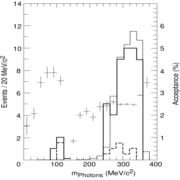
Figure 6.3: $\gamma\gamma$-invariant mass distributions of the 50 unambiguously $K_{L}\rightarrow\pi^{0}\gamma\gamma$ events reconstructed by NA31 [52] (histograms). The dashed line shows the estimated background. The dotted line simulates the ${\cal O}(E^{4})$ ChPTh prediction. Crosses indicate the experimental acceptance (scale on the right).

Several authors [50, 36, 53, 54, 55] have calculated the contribution of the on-shell two-photon intermediate state to $K_{L}\rightarrow\pi^{0}e^{+}e^{-}$. Although this is sometimes referred to as the absorption contribution, it is not the full absorption part since there is a further cut due to on-shell pions. Besides this, the full CP-conserving amplitude also receives contribution form the dispersive part of the amplitude, with off-shell photons (and pions). The calculation of this is complicated by the sensitivity of the loop integral to high momentum, as the Feynman diagram of Fig. 14 will diverge if we treat the $B$ amplitude as a constant in $q^{2}_{1}$ and $q^{2}_{2}$. However, the remedy to this is well known; the couplings of virtual photons to hadrons is governed by form factors which lead to suppression of the couplings at high $q^{2}$. We will include an estimate of these form factors and this will allow us to calculate the dispersive component of the CP-conserving amplitude.

The two-photon loop integral in the limit $m_{e}\rightarrow 0$ is given by

$${\cal M}(K_{L}\rightarrow\pi^{0}e^{+}e^{-})_{\rm CPC} = {G_{8}\alpha\over 4\pi m^{2}_{K}}\int{d^{4}\ell\over(2\pi)^{4}}{B(k+k^{\prime})F(\ell+k)F(\ell-k^{\prime})\over\ell^{2}(\ell+k)^{2}(\ell-k^{\prime})^{2}}$$

$$\times \left\{\hbox to0.0pt{/\hss}{p^{\phantom{l}}_{K}}\left[\ell^{2}+p^{\phantom{l}}_{K}\cdot(k-k^{\prime})-p^{\phantom{l}}_{K}\cdot\ell\;\ell\cdot(k-k^{\prime})\right.\right.$$

$$+ \left.\left.2p^{\phantom{l}}_{K}\cdot\ell\;k\cdot k^{\prime}-p^{\phantom{l}}_{K}\cdot k\;\ell\cdot k^{\prime}-p^{\phantom{l}}_{K}\cdot k^{\prime}\;\ell\cdot k\right]\right.$$

$$+ \left.\hbox to0.0pt{/\hss}{\ell}\left[(p^{\phantom{l}}_{K}\cdot\ell)^{2}+p^{\phantom{l}}_{K}\cdot\ell\;p^{\phantom{l}}_{K}\cdot(k-k^{\prime})\right]\right\}.$$

Here $F(q^{2})$ are the form factors for the virtual photon couplings. The structure above is certainly an approximation, as in general the virtual photon dependence need not be only an overall factor of $F(q^{2})$. However, the above form would be sufficient to capture the kinematic variation if only one photon is off-shell [given an appropriate $F(q^{2})$]. Since we only need a minor form factor suppression to tame the logarithmic divergences, we feel that this structure will be sufficient for our estimate. We choose

$$F(q^{2})={-m^{2}_{V}\over{q^{2}-m^{2}_{V}}},$$ (6.5)

which is a good representation of almost any mesonic form factor, with $m^{\phantom{\dagger}}_{V}\approx m_{\rho}$. Neglecting terms that are suppressed by powers of $1/m^{2}_{\rho}$, we find the amplitude of Eq. 6.1 above, with

$$K={B(x)\over{16\pi^{2}m^{2}_{K}}}\left[{2\over 3}\log\left({m^{2}_{\rho}}\over{-s}\right)-{1\over 4}\log\left({-s}\over{m^{2}_{e}}\right)+{7\over{18}}\right],$$ (6.6)

where $s=\left(k+k^{\prime}\right)^{2}$. The log factor is of course expected, since the photon “absorptive” part comes from the expansion $\log(-s)=\log s+i\pi$.

This representation of the amplitude leads to a CP-conserving branching ratio of

$$BR(K_{L}\rightarrow\pi^{0}e^{+}e^{-})_{\rm CPC}=4.89\times 10^{-12}$$ (6.7)

for $a^{\phantom{l}}_{V}=-0.96$. More generally we show the CP-conserving branching ratio vs. $a^{\phantom{l}}_{V}$ in Fig. 17. Note that while for many values of $a^{\phantom{l}}_{V}$ the CP-conserving rate is small compared to the CP-violating rate of previous chapters, these two rates are comparable for some range of parameters. Note that there is no interference in the rate between the CP-conserving and violating components, so that the rates just add, as shown in Fig. 18. However, there can be a CP-odd asymmetry in the electron positron energies, to which we turn in the next chapter.

Figure 6.4: The CP-conserving branching ratio $BR(K_{L}\rightarrow\pi^{0}e^{+}e^{-})_{\rm CPC}$ is plotted against $a_{V}$. The convention for the solid and dashed curves is the same as for Fig. 9. The assumed value for $a_{V}$ is indicated by the dashed vertical line.

Figure 6.5: The complete branching ratio $BR(K_{L}\rightarrow\pi^{0}e^{+}e^{-})$ is plotted against $w_{2}$. The convention for the solid and dashed curves is the same as for Fig. 9. $a_{V}=-0.96$ is assumed.

Chapter 7 THE ELECTRON ENERGY ASYMMETRY AND TIME-DEPENDENT INTERFERENCE

7.1 The Electron Energy Asymmetry

When both CP-violating and CP-conserving amplitudes contribute to the decay, there will be an asymmetry in the electron-positron energy distribution

$$A={N(E_{+}>E_{-})-N(E_{+}<E_{-})\over N(E_{+}>E_{-})+N(E_{+}<E_{-})}.$$ (7.1)

This will be quite large if the two amplitudes are comparable. In contrast to the overall decay rate, this asymmetry is an unambiguous signal of CP violation. It may be even more useful if it can be used to prove the existence of direct CP violation. This can occur because the asymmetry is sensitive to the phase of the CP-violating amplitude, and mass matrix CP violation has a unique phase (that of $\epsilon$), while direct CP violation will in general have a different phase.

For the electron energy asymmetry to be useful as a diagnostic of the form of CP violation, the CP-conserving two-photon amplitudes must be well known. As we discussed in the previous chapter, it is reasonable to expect that this will be true in the future after further phenomenology of $K_{L}\rightarrow\pi^{0}\gamma\gamma$. For illustrative purposes, we will use $a^{\phantom{l}}_{V}=-0.96$. The analysis below will need to be redone in the future if this value of $a^{\phantom{l}}_{V}$ changes significantly. However, the pattern of the analysis and the general conclusions will be valid for a wide range of values of $a^{\phantom{l}}_{V}$.

The amplitudes involved have been given in the previous chapter. Note that the two-photon amplitude has both real and imaginary parts, the mass matrix CP-violating amplitude has a phase of $45^{o}$, while the direct component is purely imaginary. The asymmetry is proportional to the imaginary part of $B$ times the real part of $d_{V}$ minus the product of the real part of $B$ and imaginary part of $d_{V}$. The asymmetry may be defined in differential form:

$${d\Gamma\over dz}(E_{+}>E_{-}) = \int_{0}^{{1\over 2}\lambda^{{1\over 2}}(1,z,r^{2})}dy{d\Gamma\over dydz},$$

$${d\Gamma\over dz}(E_{+}<E_{-}) = \int^{0}_{-{1\over 2}\lambda^{{1\over 2}}(1,z,r^{2})}dy{d\Gamma\over dydz},$$

$$\lambda(1,z,r^{2}) = 1+z^{2}+r^{4}-2z-2r^{2}-2r^{2}z,$$

$$r = {m_{\pi}\over m_{K}},$$

$$A(z) \equiv {{d\Gamma(E_{+}>E_{-})/dz-d\Gamma(E_{+}<E_{-})/dz}\over{d\Gamma(E_{+}>E_{-})/dz+d\Gamma(E_{+}<E_{-})/dz}},$$

$$z \equiv (k+k^{\prime})^{2}/m^{2}_{K}.$$ (7.2)

In Fig. 19 we plot the differential asymmetry for several values of $w_{2}$ in the case when there is no direct CP violation. Fig. 20 gives the same information for ${\rm Im}\lambda_{t}=10^{-4}$. We see that the asymmetry is sizable for many values of $w^{\phantom{2}}_{2}$ and that it depends significantly on direct CP violation, even possibly changing sign. The integrated asymmetry is plotted versus $w_{2}$ in Figs. 21, 22.

Figure 7.1: The differential asymmetry $A(K_{L}\rightarrow\pi^{0}e^{+}e^{-})$ is plotted against $z\equiv(k+k^{\prime})^{2}/m^{2}_{K}$ for $w_{2}$ = 1 $\times 10^{-2}$ (curve 1), 2 $\times 10^{-2}$ (curve 2), $\dots$, 5 $\times 10^{-2}$ (curve 5), in the case when there is no direct CP violation. $a_{V}=-0.96$ is assumed.

Figure 7.2: Same as Fig. 19 for ${\rm Im}\lambda_{t}$ = $10^{-4}$.

Figure 7.3: The integrated asymmetry is plotted vs. $w_{2}$ in the case when there is no direct CP violation. The convention for the solid and dashed curves is the same as for Fig. 9. $a_{V}=-0.96$ is assumed.

Figure 7.4: Same as Fig. 21 for ${\rm Im}\lambda_{t}$ = $10^{-4}$.

Both the decay rate and the asymmetry depend on $w^{\phantom{2}}_{S}$ and this forms the main uncertainty in the analysis. However, it is possible to remove this uncertainty by measuring both observables. For a given value of the CP-conserving amplitude, there is a strict correlation between the two. In Fig. 23 we plot the values of the branching ratio and the integrated asymmetry $A$ as one varies $w_{2}$. We see that the curves with and without direct CP violation are well separated for much of the range. To the extent that we understand the CP-conserving amplitude, this can be used as a diagnostic test for direct CP violation.

Figure 7.5: The integrated asymmetry $A(K_{L}\rightarrow\pi^{0}e^{+}e^{-})$ is plotted vs. the branching ratio $BR(K_{L}\rightarrow\pi^{0}e^{+}e^{-})$ as one varies $w_{2}$. $a_{V}=-0.96$ is assumed. The solid curve describes the case when there is no direct CP violation, the dashed curve is for ${\rm Im}\lambda_{t}$ = $10^{-4}$.

7.2 Time-Dependent Interference of $K_{1}$, $K_{2}$ $\rightarrow\pi^{0}e^{+}e^{-}$

Littenberg [56] has suggested a time-dependent analysis of a state starting out as a $K^{0}$ in order to extract maximal information about the decay mechanism. This is far more demanding experimentally then simply measuring $K_{L}$ or $K_{S}$ decays separately. However, we analyze this technique in order to assess its usefulness.

A state that at $t=0$ is a $K^{0}$ will evolve into a mixture of $K_{L}$ and $K_{S}$:

$$|K^{0}(t)\rangle={1\over{(1+\epsilon)\sqrt{2}}}\left\{e^{-iH^{\phantom{l}}_{S}t}\left[|K_{1}\rangle+\epsilon|K_{2}\rangle\right]+e^{-iH^{\phantom{l}}_{L}t}\left[|K_{2}\rangle+\epsilon|K_{1}\rangle\right]\right\},$$ (7.3)

where

$$H^{\phantom{l}}_{j}=m^{\phantom{l}}_{j}-i{\Gamma_{j}\over 2},\qquad j={\rm S,L}.$$ (7.4)

Ignoring small effects such as second order CP violation and direct CP-violating components in the parameter $\epsilon$, we then have a time development proportional to

$$|\langle\pi^{0}e^{+}e^{-}\left|{\cal H}\right|K^{0}(t)\rangle|^{2} \approx {1\over 2}\left\{\left|A^{\phantom{l}}_{S}\right|^{2}e^{-\Gamma^{\phantom{l}}_{S}t}+\left|\epsilon A_{S}+A_{\rm dir}+A_{\rm CPC}\right|^{2}e^{-\Gamma^{\phantom{l}}_{L}t}\phantom{e^{-{(\Gamma^{\phantom{l}}_{L}+\Gamma^{\phantom{l}}_{S})t}\over 2}}\right.$$

$$+ \left.2{\rm Re}\left[\left(\epsilon A^{\phantom{l}}_{S}+A_{\rm dir}+A_{\rm CPC}\right)A^{*}_{S}e^{-i(m^{\phantom{l}}_{L}-m^{\phantom{l}}_{S})t}\right]e^{-{{(\Gamma^{\phantom{l}}_{L}+\Gamma^{\phantom{l}}_{S})t}\over 2}}\right\}.$$

(7.5)

Here $A_{\rm dir}$, $\epsilon A_{S}$ and $A_{\rm CPC}$ are the amplitudes analyzed in chapters 3, 4 and 6 respectively. Measurements at early time $(t\ll 1/\Gamma_{S})$ determine $\Gamma(K_{S}\rightarrow\pi^{0}e^{+}e^{-})$ while at the late time $(t\gg 1/\Gamma_{S})$ one observes $\Gamma(K_{L}\rightarrow\pi^{0}e^{+}e^{-})$. These contain the information described in preceding chapters. However, in the interference region $t$ = ${\cal O}\left({1/(m^{\phantom{l}}_{L}-m^{\phantom{l}}_{S})}\right)$ $\sim$ ${\cal O}(1/\tau^{\phantom{\dagger}}_{S})$, we obtain extra information about the separate contributions to the decay amplitude.

In Fig. 24 we show the time-dependent signal for the cases of pure mass matrix CP violation and the addition of direct CP violation, using the analysis of the previous chapters with $w_{2}=4L_{9}$. We see that the shape of the interference region does differentiate these two cases, but that for the case studied the dependence on direct CP violation is not so large as to allow an easy experimental determination.

Figure 7.6: The normalized time distribution of $K^{0}\rightarrow\pi^{0}e^{+}e^{-}$ decays is plotted vs. time $t$ in nsecs. $a_{V}=-0.96$ is assumed. The solid curve describes the case when there is no direct CP violation, the dashed curve is for ${\rm Im}\lambda_{t}$ = $10^{-4}$.

Chapter 8 THE $\cal{O}$(E⁴) CALCULATION

First let us provide the straightforward $\cal{O}$(E⁴) calculation of ${\cal M}(K_{L}\rightarrow\pi^{0}\gamma e^{+}e^{-})$ within ChPTh. This is the generalization to $k^{2}_{1}\neq 0$ of the original chiral calculation of EPR [34, 35]. Here $k_{1}$ is the momentum of the off-shell photon. This captures all the $k^{2}_{1}/m^{2}_{\pi}$ and $k^{2}_{1}/m^{2}_{K}$ variations of the amplitudes at this order in the energy expansion. There can be further $k^{2}_{1}$/(1 GeV)² corrections which correspond to $\cal{O}$(E⁶) and higher. The easiest technique for this calculation uses the basis where the kaon and pion fields are transformed so that the propagators have no off-diagonal terms, as described in Ref. [34, 35]. The relevant diagrams are then shown in Fig. 25. Defining $\overline{g}$ as

$${\overline{g}}=G^{\phantom{l}}_{8}/3,\qquad\qquad G^{\phantom{l}}_{8}=G^{\phantom{l}}_{F}|V_{ud}^{\phantom{*}}V_{us}^{*}|g^{\phantom{l}}_{8},\qquad\qquad|g^{\phantom{l}}_{8}|\approx 5.1,$$ (8.1)

the diagrams give the following integrals, respectively:

$${\cal M}^{a}_{\mu\nu}=2e^{2}{\overline{g}}g_{\mu\nu}\int{{d^{4}l}\over{(2\pi)^{4}}}{{3[(p^{\phantom{l}}_{K}-p^{\phantom{l}}_{0})^{2}-m^{2}_{\pi}]-2[(l^{2}-m^{2}_{\pi})+(l-k_{1}-k_{2})^{2}-m^{2}_{\pi}]}\over{(l^{2}-m^{2}_{\pi})[(l-k_{1}-k_{2})^{2}-m^{2}_{\pi}]}},$$ (8.2)

$${\cal M}^{b}_{\mu\nu} = -e^{2}{\overline{g}}\int{{d^{4}l}\over{(2\pi)^{4}}}{{3[(p^{\phantom{l}}_{K}-p^{\phantom{l}}_{0})^{2}-m^{2}_{\pi}]-2[(l+k_{1})^{2}-m^{2}_{\pi}+(l-k_{2})^{2}-m^{2}_{\pi}]}\over{(l^{2}-m^{2}_{\pi})[(l+k_{1})^{2}-m^{2}_{\pi}][(l-k_{2})^{2}-m^{2}_{\pi}]}}$$ (8.3)

$$\times (2l+k_{1})_{\mu}(2l-k_{2})_{\nu}+(k_{1},\mu)\leftrightarrow(k_{2},\nu),$$

$${\cal M}^{c}_{\mu\nu}=8e^{2}{\overline{g}}g_{\mu\nu}\int{{d^{4}l}\over{(2\pi)^{4}}}{1\over{l^{2}-m^{2}_{\pi}}},$$ (8.4)

$${\cal M}^{d}_{\mu\nu}=-4e^{2}{\overline{g}}\int{{d^{4}l}\over{(2\pi)^{4}}}\left\{{{(2l-k_{1})_{\mu}(2l-k_{1})_{\nu}}\over{(l^{2}-m^{2}_{\pi})[(l-k_{1})^{2}-m^{2}_{\pi}]}}+{{(2l-k_{2})_{\mu}(2l-k_{2})_{\nu}}\over{(l^{2}-m^{2}_{\pi})[(l-k_{2})^{2}-m^{2}_{\pi}]}}\right\}.$$ (8.5)

Figure 8.1: Diagrams relevant to the process $K_{L}\rightarrow\pi^{0}\gamma e^{+}e^{-}$ at ${\cal O}(E^{4})$ and ${\cal O}(E^{6})$.

Interestingly when we add these together the $K\rightarrow 3\pi$ amplitude factors out from the remaining loop integral resulting in

$${\cal M}^{\pi}_{\mu\nu}=6e^{2}{\overline{g}}[(p^{\phantom{l}}_{K}-p^{\phantom{l}}_{0})^{2}-m^{2}_{\pi}]\int{{d^{4}l}\over{(2\pi^{4})}}{{[g_{\mu\nu}(l^{2}-m^{2}_{\pi})-(2l+k_{1})_{\mu}(2l-k_{2})_{\nu}]}\over{{(l^{2}-m^{2}_{\pi})[(l+k_{1})^{2}-m^{2}_{\pi}][(l-k_{2})^{2}-m^{2}_{\pi}]}}}.$$ (8.6)

It is not hard to verify that this result satisfies the constraints of gauge invariance $k^{\mu}_{1}\cal{M}_{\mu\nu}$ = $k^{\nu}_{2}\cal{M}_{\mu\nu}$ = 0. At this stage, the integral may be parametrized and integrated using standard Feynman-diagram techniques. Let us keep photon number one as the off-shell photon and set $k^{2}_{2}=0$. In this case the amplitude with one photon off-shell is described by

$${\cal M}^{\pi}_{\mu\nu}=6e^{2}{\overline{g}}[(p^{\phantom{l}}_{K}-p^{\phantom{l}}_{0})^{2}-m^{2}_{\pi}]\left({-i}\over{16\pi^{2}}\right){{(g_{\mu\nu}k_{1}\cdot k_{2}-k_{2\mu}k_{1\nu})}\over{k_{1}\cdot k_{2}}}[1+2I(m^{2}_{\pi})],$$ (8.7)

with

$$I(m^{2}_{\pi}) = \int^{1}_{0}dz_{1}\int_{0}^{1-z_{1}}dz_{2}{{m^{2}_{\pi}-z_{1}(1-z_{1})k^{2}_{1}}\over{2z_{1}z_{2}k_{1}\cdot k_{2}+z_{1}(1-z_{1})k^{2}_{1}-m^{2}_{\pi}+i\epsilon}}$$ (8.8)

$$= {m^{2}_{\pi}\over{s-k^{2}_{1}}}[F(s)-F(k^{2}_{1})]-{k^{2}_{1}\over{s-k^{2}_{1}}}[G(s)-G(k^{2}_{1})].$$

The notation is defined by

$$s=(p^{\phantom{l}}_{K}-p^{\phantom{l}}_{0})^{2}=(k_{1}+k_{2})^{2}$$ (8.9)

and

$$F(a)=\int^{1}_{0}{dz_{1}\over z_{1}}\log\left[{{m^{2}_{\pi}-a(1-z_{1})z_{1}-i\epsilon}\over{m^{2}_{\pi}}}\right],$$ (8.10)

$$G(a)=\int^{1}_{0}dz_{1}\log\left[{{m^{2}_{\pi}-a(1-z_{1})z_{1}-i\epsilon}\over{m^{2}_{\pi}}}\right].$$ (8.11)

The above functions are related to those presented by CEP [36]:

$$F(a)={a\over{2m^{2}_{\pi}}}\left[F_{\rm CEP}\left({a\over 4m^{2}_{\pi}}\right)-1\right],$$ (8.12)

$$G(a)=-{a\over{2m^{2}_{\pi}}}\left[R_{\rm CEP}\left({a\over 4m^{2}_{\pi}}\right)+{1\over 6}\right],$$ (8.13)

remembering Eq. 6:

$$F_{\rm CEP}(x) = 1-{1\over x}\left[\arcsin\left(\sqrt{x}\right)\right]^{2},\,\qquad x\leq 1,$$

$$= 1+{1\over 4x}\left(\log{1-\sqrt{1-1/x}\over 1+\sqrt{1-1/x}}+i\pi\right)^{2},\,\qquad x\geq 1,$$

$$R_{\rm CEP}(x) = -{1\over 6}+{1\over 2x}\left[1-\sqrt{1/x-1}\arcsin\left(\sqrt{x}\right)\right],\,\qquad x\leq 1,$$

$$-{1\over 6}+{1\over 2x}\left[1+\sqrt{1-1/x}\left(\log{1-\sqrt{1-1/x}\over 1+\sqrt{1-1/x}}+i\pi\right)\right],\,\qquad x\geq 1.$$

(8.14)

This agrees with the EPR result in the $k^{2}_{1}\rightarrow 0$ limit.

At this order we have also calculated the additional contribution resulting from the kaons circulating in the loops of Fig. 25. They give rise to

$${\cal M}^{K}_{\mu\nu}=6e^{2}{\overline{g}}(m^{2}_{K}+m^{2}_{\pi}-s)\int{{d^{4}l}\over{(2\pi^{4})}}{{[g_{\mu\nu}(l^{2}-m^{2}_{K})-(2l+k_{1})_{\mu}(2l-k_{2})_{\nu}]}\over{{(l^{2}-m^{2}_{K})[(l+k_{1})^{2}-m^{2}_{K}][(l-k_{2})^{2}-m^{2}_{K}]}}}.$$ (8.15)

The resulting integral is similar to that of Eq. 8.8, substituting the mass of the pion with that of the kaon. Attaching an $e^{+}e^{-}$ couple to either photon and adding all the above contributions together, the result we obtain for the branching ratio is

$${\rm BR}(K_{L}\rightarrow\pi^{0}\gamma e^{+}e^{-})=1.0\times 10^{-8}.$$ (8.16)

With the definitions

$$z={s\over{m^{2}_{K}}},\qquad y={{p^{\phantom{l}}_{K}\cdot(k_{1}-k_{2})}\over{m^{2}_{K}}},$$ (8.17)

the decay distributions in $z$ and $y$ provide more detailed information. We present them in Figs. 26 and 27.

Figure 8.2: Differential branching ratio $dBR(K_{L}\rightarrow\pi^{0}\gamma e^{+}e^{-})/dz$ to ${\cal O}$(E⁴).

Figure 8.3: Differential branching ratio $dBR(K_{L}\rightarrow\pi^{0}\gamma e^{+}e^{-})/dy$ to ${\cal O}$(E⁴).

Chapter 9 THE $\cal{O}$(E⁶) CALCULATION

We also wish to extend this calculation along the lines proposed by CEP [36], who provide a plausible solution to the problem raised by the experimental rate not agreeing with the $\cal{O}$(E⁴) calculation when both photons are on-shell. The two primary new ingredients involve known physics that surfaces at the next order in the energy expansion. The first involves the known quadratic energy variation of the $K\rightarrow 3\pi$ amplitude, which occurs from higher order terms in the weak nonleptonic lagrangian [51, 55, 57]. While the full one-loop structure of this is known [48, 49, 58], it involves complicated nonanalytic functions and we approximate the result at $\cal{O}$(E⁴) by an analytic polynomial which provides a good description of the data throughout the physical region:

$${\cal M}(K\rightarrow\pi^{+}\pi^{-}\pi^{0})=4a_{1}p^{\phantom{l}}_{K}\cdot p^{\phantom{l}}_{0}p^{\phantom{l}}_{+}\cdot p^{\phantom{l}}_{-}+4a_{2}(p^{\phantom{l}}_{K}\cdot p^{\phantom{l}}_{+}p^{\phantom{l}}_{0}\cdot p^{\phantom{l}}_{-}+p^{\phantom{l}}_{K}\cdot p^{\phantom{l}}_{-}p^{\phantom{l}}_{0}\cdot p^{\phantom{l}}_{+}),$$ (9.1)

using

$$a_{1}=3.1\times 10^{-6}m^{-4}_{K}\qquad{\rm and}\qquad a_{2}=-1.26\times 10^{-6}m^{-4}_{K}.$$ (9.2)

$a_{1}$ and $a_{2}$ are obtained from a fit to the amplitude for $K_{L}\rightarrow\pi^{0}\pi^{+}\pi^{-}$ [51] and to the amplitude and spectrum for $K_{L}\rightarrow\pi^{0}e^{+}e^{-}$ [36], so that their values are constrained within their theoretical uncertainty of 10 – 20%. We have numerically verified that such a variation of said parameters involves a very modest change in the shape of the spectrum for $K_{L}\rightarrow\gamma\pi^{0}e^{+}e^{-}$ and a change in its final branching ratio somewhat smaller than the uncertainty on the parameters.

The other ingredient involves vector meson exchange such as in Fig. 28. Some of such contributions are known, but there are others such as those depicted in Fig. 29 which have the same structure but an unknown strength, leaving the total result unknown. In Ref. [36] the result is parametrized by a “subtraction constant” that must be fit to the data.

Figure 9.1: Vector meson exchange diagrams contributing to $K_{L}\rightarrow\pi^{0}\gamma e^{+}e^{-}$.

Figure 9.2: Vector meson exchange diagrams contributing to $K_{L}\rightarrow\pi^{0}\gamma e^{+}e^{-}$ with unknown strength.

In principle one can add the ingredients to the amplitudes and perform a dispersive calculation of the total transition matrix element. In practice it is simple to convert the problem into an effective field theory and and do a Feynman-diagram calculation which will yield the same result. We follow this latter course.

The Feynman diagrams are the same as shown in Fig. 25, although the vertices are modified by the presence of $\cal{O}$(E⁴) terms in the energy expansion. Not only does the direct $K\rightarrow 3\pi$ vertex change to the form given in Eq. 9.1, but also the weak vertices with one and two photons have a related change. The easiest way to determine these is to write a gauge invariant effective lagrangian with coefficients adjusted to reproduce Eq. 9.1. We find

$${\cal M_{\mu}}(K\rightarrow\pi^{+}\pi^{-}\pi^{0}\gamma)=4a_{1}e(p^{\phantom{l}}_{+}-p^{\phantom{l}}_{-})_{\mu}p^{\phantom{l}}_{K}\cdot p^{\phantom{l}}_{0}+4a_{2}e(p^{\phantom{l}}_{+}-p^{\phantom{l}}_{-})_{\sigma}(p^{\sigma}_{0}p^{\phantom{l}}_{K\mu}+p^{\sigma}_{K}p^{\phantom{l}}_{0\mu}),$$ (9.3)

$${\cal M}_{\mu\nu}(K\rightarrow\pi^{+}\pi^{-}\pi^{0}\gamma\gamma)=-8a_{1}e^{2}g_{\mu\nu}p^{\phantom{l}}_{K}\cdot p^{\phantom{l}}_{0}+8a_{2}e^{2}(p^{\phantom{l}}_{K\mu}p^{\phantom{l}}_{0\nu}+p^{\phantom{l}}_{K\nu}p^{\phantom{l}}_{0\mu}).$$ (9.4)

The resulting calculation follows the same steps as described above, but is more involved and is not easy to present in a simple form. We have checked that our result is gauge invariant and reduces to that of CEP in the limit of on-shell photons.

The contribution proportional to $a_{1}$ can be computed analogously to those already calculated for the $\cal{O}$(E⁴) case:

$${\cal M}_{\mu\nu}=4a_{1}e^{2}(z-2r^{2}_{\pi})(1+r^{2}_{\pi}-z){1\over{z-q}}(g_{\mu\nu}k_{1}\cdot k_{2}-k_{2\mu}k_{1\nu})[1+2I(m^{2}_{\pi})],$$ (9.5)

where

$$r_{\pi}={m_{\pi}\over m_{K}},\qquad z={s\over{m^{2}_{K}}},\qquad q={{k^{2}_{1}}\over{m^{2}_{K}}}.$$ (9.6)

The $a_{2}$ part originates another set of integrals which can be written as

$${\cal M}^{a}_{\mu\nu}=-8a_{2}(p^{\rho}_{K}p^{\sigma}_{0}+p^{\sigma}_{K}p^{\rho}_{0})e^{2}g_{\mu\nu}\int{{d^{d}l}\over{(2\pi)^{d}}}{{l_{\rho}(l-k_{1}-k_{2})_{\sigma}}\over{(l^{2}-m^{2}_{\pi})[(l-k_{1}-k_{2})^{2}-m^{2}_{\pi}]}},$$ (9.7)

$${\cal M}^{b}_{\mu\nu}\hskip-0.4pt = \hskip-0.4pt4a_{2}(p^{\rho}_{K}p^{\sigma}_{0}+p^{\sigma}_{K}p^{\rho}_{0})e^{2}\int{{d^{d}l}\over{(2\pi)^{d}}}\left\{{{(2l+k_{1})_{\mu}(2l-k_{2})_{\nu}(l+k_{1})_{\rho}(l-k_{2})_{\sigma}}\over{(l^{2}-m^{2}_{\pi})[(l+k_{1})^{2}-m^{2}_{\pi}][(l-k_{2})^{2}-m^{2}_{\pi}]}}\right.$$

$$+ \hskip-0.4pt\left.{{(2l+k_{2})_{\nu}(2l-k_{1})_{\mu}(l+k_{2})_{\rho}(l-k_{1})_{\sigma}}\over{(l^{2}-m^{2}_{\pi})[(l-k_{1})^{2}-m^{2}_{\pi}][(l+k_{2})^{2}-m^{2}_{\pi}]}}\right\}$$

$$= \hskip-0.4pt8a_{2}(p^{\rho}_{K}p^{\sigma}_{0}+p^{\sigma}_{K}p^{\rho}_{0})e^{2}\int{{d^{d}l}\over{(2\pi)^{d}}}{{(2l+k_{1})_{\mu}(2l-k_{2})_{\nu}(l+k_{1})_{\rho}(l-k_{2})_{\sigma}}\over{(l^{2}-m^{2}_{\pi})[(l+k_{1})^{2}-m^{2}_{\pi}][(l-k_{2})^{2}-m^{2}_{\pi}]}},$$

(9.8)

$${\cal M}^{c}_{\mu\nu}=8a_{2}(p^{\phantom{l}}_{K\mu}p^{\phantom{l}}_{0\nu}+p^{\phantom{l}}_{K\nu}p^{\phantom{l}}_{0\mu})e^{2}\int{{d^{d}l}\over{(2\pi)^{d}}}{1\over{l^{2}-m^{2}_{\pi}}},$$ (9.9)

$${\cal M}^{d}_{\mu\nu} = -4a_{2}(p^{\sigma}_{0}p^{\phantom{l}}_{K\nu}+p^{\sigma}_{K}p^{\phantom{l}}_{0\nu})e^{2}\int{{d^{d}l}\over{(2\pi)^{d}}}{{(2l-k_{1})_{\mu}(2l-k_{1})_{\sigma}}\over{(l^{2}-m^{2}_{\pi})[(l-k_{1})^{2}-m^{2}_{\pi}]}}$$ (9.10)

$$- 4a_{2}(p^{\sigma}_{0}p^{\phantom{l}}_{K\mu}+p^{\sigma}_{K}p^{\phantom{l}}_{0\mu})e^{2}\int{{d^{d}l}\over{(2\pi)^{d}}}{{(2l-k_{2})_{\nu}(2l-k_{2})_{\sigma}}\over{(l^{2}-m^{2}_{\pi})[(l-k_{2})^{2}-m^{2}_{\pi}]}}.$$

From the above formulas we obtain

$${\cal M}_{\mu\nu}\hskip-4.0pt = \hskip-4.0pt{1\over{(4\pi)^{2}}}\left[A(x_{1},x_{2})(k_{2\mu}k_{1\nu}-k_{1}\cdot k_{2}g_{\mu\nu})\phantom{{k^{2}_{1}}\over{k_{1}}}\right.$$

$$+ \hskip-4.0ptB(x_{1},x_{2})\left({p^{\phantom{l}}_{K}\cdot k_{1}p^{\phantom{l}}_{K}\cdot k_{2}\over{k_{1}\cdot k_{2}}}g_{\mu\nu}+p^{\phantom{l}}_{K\mu}p_{K\nu}-{{p^{\phantom{l}}_{K}\cdot k_{1}}\over{k_{1}\cdot k_{2}}}k_{2\mu}p^{\phantom{l}}_{K\nu}-{{p^{\phantom{l}}_{K}\cdot k_{2}}\over{k_{1}\cdot k_{2}}}k_{1\nu}p^{\phantom{l}}_{K\mu}\right)$$

$$+ \hskip-4.0pt\left.D(x_{1},x_{2})\left(k^{2}_{1}{p^{\phantom{l}}_{K}\cdot k_{2}\over{k_{1}\cdot k_{2}}}g_{\mu\nu}-{{p^{\phantom{l}}_{K}\cdot k_{2}}\over{k_{1}\cdot k_{2}}}k_{1\mu}k_{1\nu}+k_{1\mu}p^{\phantom{l}}_{K\nu}-{{k^{2}_{1}}\over{k_{1}\cdot k_{2}}}k_{2\mu}p^{\phantom{l}}_{K\nu}\right)\right],$$

(9.11)

where

$${A\over m^{2}_{K}}\hskip-4.5pt = \hskip-4.5pt16a_{2}e^{2}\{2[1-2(x_{1}+x_{2})]I_{1}(z_{1}z_{2})+x_{1}I_{1}(z_{2})+x_{2}[2I_{1}(z^{2}_{2})-I_{1}(z_{2})+I_{1}(z_{1})]\}$$ (9.12)

$$- \hskip-4.5pt32a_{2}e^{2}\{[2x^{2}_{1}-x_{1}(z+q)][-I_{2}(z^{3}_{1}z_{2})+I_{2}(z^{2}_{1}z_{2})]$$

$$+ \hskip-4.5pt[2x_{1}x_{2}-x_{1}(z-q)/2-x_{2}(z+q)/2][2I_{2}(z^{2}_{1}z^{2}_{2})+I_{2}(z_{1}z_{2})-I_{2}(z^{2}_{1}z_{2})$$

$$- \hskip-4.5ptI_{2}(z_{1}z^{2}_{2})]+[2x^{2}_{2}-x_{2}(z-q)][I_{2}(z_{1}z^{2}_{2})-I_{2}(z_{1}z^{3}_{2})]\}$$

$$+ \hskip-4.5pt{4\over 3}a_{2}e^{2}\left(1+\log{m^{2}_{\pi}\over{m^{2}_{\rho}}}\right)+(4\pi)^{2}{\rm VMD}_{A},$$

$${B\over m^{2}_{K}}=-32a_{2}e^{2}I_{3}+16a_{2}e^{2}I_{4}+{4\over 3}a_{2}e^{2}(z-q)\log{m^{2}_{\pi}\over{m^{2}_{\rho}}}+(4\pi)^{2}{\rm VMD}_{B},$$ (9.13)

$${D\over m^{2}_{K}} = 16a_{2}e^{2}I_{3}-8a_{2}e^{2}I_{4}-{2\over 3}a_{2}e^{2}(z-q)\log{m^{2}_{\pi}\over{m^{2}_{\rho}}}$$ (9.14)

$$+ 16a_{2}e^{2}[2x_{2}-(z-q)/2][2I_{1}(z_{1}z_{2})-I_{1}(z_{2})]$$

$$+ 16a_{2}e^{2}(2y-q)[I_{1}(z_{1})-I_{1}(1)/2]+4a_{2}e^{2}[2x_{1}-(z+q)/2]I_{5}$$

$$+ (4\pi)^{2}{\rm VMD}_{D},$$

with the integrals given in the Appendix:

$$I_{1}(z^{n}_{1}z^{m}_{2})=\int^{1}_{0}dz_{1}\int^{1-z_{1}}_{0}dz_{2}z^{n}_{1}z^{m}_{2}\log{D_{1}\over{m^{2}_{\pi}}},$$ (9.15)

$${I_{2}(z^{n}_{1}z^{m}_{2})\over m^{2}_{K}}=\int^{1}_{0}dz_{1}\int^{1-z_{1}}_{0}dz_{2}{{z^{n}_{1}z^{m}_{2}}\over D_{1}},$$ (9.16)

$$I_{3}m^{2}_{K}=\int^{1}_{0}dz_{1}\int^{1-z_{1}}_{0}dz_{2}D_{1}\log{D_{1}\over{m^{2}_{\pi}}},$$ (9.17)

$$I_{4}m^{2}_{K}=\int^{1}_{0}dz_{1}D_{2}\log{D_{2}\over{m^{2}_{\pi}}},$$ (9.18)

$$I_{5}=\int^{1}_{0}dz_{1}(4z^{2}_{1}-4z_{1}+1)\log{D_{2}\over{m^{2}_{\pi}}},$$ (9.19)

and

$$D_{1} = m^{2}_{\pi}-2k_{1}\cdot k_{2}z_{1}z_{2}-k^{2}_{1}z_{1}(1-z_{1}),$$

$$D_{2} = m^{2}_{\pi}-k^{2}_{1}z_{1}(1-z_{1}),$$

$$x_{1} = {{p^{\phantom{l}}_{K}\cdot k_{1}}\over{m^{2}_{K}}},\qquad x_{2}={{p^{\phantom{l}}_{K}\cdot k_{2}}\over{m^{2}_{K}}},$$ (9.20)

$${\rm VMD}_{A}(x_{1},x_{2})=-\sum_{V=\omega,\rho}G_{V}\left[{{p^{\phantom{l}}_{K}\cdot(p^{\phantom{l}}_{K}-k_{2})}\over{(p^{\phantom{l}}_{K}-k_{2})^{2}-m^{2}_{V}}}+{{p^{\phantom{l}}_{K}\cdot(p^{\phantom{l}}_{K}-k_{1})}\over{(p^{\phantom{l}}_{K}-k_{1})^{2}-m^{2}_{V}}}\right],$$ (9.21)

$${\rm VMD}_{B}(x_{1},x_{2})=-\sum_{V=\omega,\rho}G_{V}k_{1}\cdot k_{2}\left[{1\over{(p^{\phantom{l}}_{K}-k_{2})^{2}-m^{2}_{V}}}+{1\over{(p^{\phantom{l}}_{K}-k_{1})^{2}-m^{2}_{V}}}\right],$$ (9.22)

$${\rm VMD}_{D}(x_{1},x_{2})=\sum_{V=\omega,\rho}G_{V}{{k_{1}\cdot k_{2}}\over{(p^{\phantom{l}}_{K}-k_{1})^{2}-m^{2}_{V}}},$$ (9.23)

assuming the numerical values [54]

$$G_{\rho}m^{2}_{K}=0.68\times 10^{-8},\qquad G_{\omega}m^{2}_{K}=-0.28\times 10^{-7}.$$ (9.24)

The loop calculation that we have just described provides all of the off-shell dependence scaled by the pion mass, and is of the form $k^{2}_{1}/m^{2}_{\pi}$. There can be an additional dependence of the form $k^{2}_{1}/\Lambda^{2}$, where $\Lambda$ $\approx$ 1 GeV. We cannot provide a model independent analysis of the latter. However, experience has shown that most of the higher order momentum dependence is well accounted for by vector meson exchange. Therefore we include the $k^{2}_{1}/\Lambda^{2}$ dependence which is predicted by the diagrams of Fig. 28. One can recover the parametrization in $a^{\phantom{l}}_{V}$ neglecting the dependence on $(p^{\phantom{l}}_{K}-k_{1})^{2}$ and $(p^{\phantom{l}}_{K}-k_{2})^{2}$ in formulas 9.21–9.23, and performing the replacement [54]

$${{\pi G_{\rm eff}m^{2}_{K}}\over{2G_{8}\alpha m^{2}_{V}}}\rightarrow a^{\phantom{l}}_{V},$$ (9.25)

where $G_{\rm eff}$ $\approx$ $G_{\rho}$+$G_{\omega}$. This completes our treatment of the $K_{L}\rightarrow\pi^{0}\gamma e^{+}e^{-}$ amplitude.

The calculation we have presented in this chapter leads to the total branching ratio of

$${\rm BR}(K_{L}\rightarrow\pi^{0}\gamma e^{+}e^{-})=2.4\times 10^{-8}.$$ (9.26)

The decay distributions are presented in Figs. 30 and 31.

Figure 9.3: Differential branching ratio $dBR(K_{L}\rightarrow\pi^{0}\gamma e^{+}e^{-})/dz$ to ${\cal O}$(E⁶).

Figure 9.4: Differential branching ratio $dBR(K_{L}\rightarrow\pi^{0}\gamma e^{+}e^{-})/dy$ to ${\cal O}$(E⁶).

Chapter 10 CONCLUSIONS

Rare kaon decays are an important testing ground of the electroweak flavor theory. With the improved experimental sensitivity expected in the near future, they can provide new signals of CP violation phenomena and an opportunity to explore physics beyond the Standard Model.

The theoretical analysis of these decays is far from trivial due to the very low mass of the hadrons involved. The delicate interplay between the flavor-changing dynamics and the confining QCD interaction makes very difficult to perform precise dynamical predictions. Fortunately, the Goldstone nature of the pseudoscalar mesons implies strong constraints on their low-energy interactions, which can be analyzed with effective lagrangian methods. The ChPTh framework incorporates all the constraints implied by the chiral symmetry of the underlying lagrangian at the quark level, allowing for a clear distinction between genuine aspects of the Standard Model and additional assumptions of variable credibility, usually related to the problem of long-distance dynamics. The low-energy amplitudes are calculable in ChPTh, except for some coupling constants that are not restricted by chiral symmetry. These constants reflect our lack of understanding of the QCD confinement mechanism and must be determined experimentally for the time being. Further progress in QCD can only improve our knowledge of these chiral constants, but it cannot modify the low-energy structure of the amplitudes.

Addressing the two specific rare decays analyzed in this thesis, we can conclude that because of the three possible contributions to $K_{L}\rightarrow\pi^{0}e^{+}e^{-}$, the analysis of this process has multiple issues that theory must address. We have provided an updated analysis of all of its components. The goal of identifying direct CP violation will not be easily accomplished. The decay rate by itself suffers from a severe uncertainty in the analysis of the mass matrix contributions. In the chiral analysis there is a free parameter, $w_{2}$, which is not fixed experimentally, and which has a strong influence on the decay rate. Measuring the related rate of $K_{S}\rightarrow\pi^{0}e^{+}e^{-}$ would determine this parameter and will likely allow us to determine whether or not direct CP violation is present.

Alternatively if the $K_{S}$ branching ratio is not measured it may be possible to signal direct CP violation using the asymmetry in the $e^{+}$, $e^{-}$ energies. The direct and mass matrix CP violations have different phases, and the asymmetry is sensitive to their difference. There exist some combinations of the parameters where there remains some ambiguity, but for sizeable portions of the parameter space direct CP violation can be signaled by a simultaneous measurement of the decay rate and the energy asymmetry, as illustrated in Fig. 23.

Progress in the theoretical analysis is possible, especially in the CP-conserving amplitude that proceeds through the two-photon intermediate state. Here both a better phenomenological understanding of the related decay $K_{L}\rightarrow\pi^{0}\gamma\gamma$, and a better theoretical treatment of the dispersive contribution should be possible in the near future.

Overall, our reanalysis shows that the demands on the experimental exploration of this reaction are quite severe. The simple observation of a few events will not be sufficient to indicate direct CP violation. The measurement of an electron asymmetry requires more events, and may or may not resolve the issue. Only the simultaneous measurement of $K_{S}\rightarrow\pi^{0}e^{+}e^{-}$ allows a convincing proof of the existence of direct CP violation.

The behavior of the $K_{L}\rightarrow\pi^{0}\gamma e^{+}e^{-}$ amplitude mirrors closely that of the process $K_{L}\rightarrow\pi^{0}\gamma\gamma$. The more complete calculation at order E⁶ gives a rate which is more than twice as large as the one obtained at order E⁴, despite the fact that the new parameter introduced at order E⁶ is quite reasonable in magnitude. This large change occurs partially because the order E⁴ calculation is purely a loop effect, while at order E⁶ we have tree level contributions, and loop contributions are generally smaller than tree effects at a given order. It was more surprising that the spectrum in $K_{L}\rightarrow\pi^{0}\gamma\gamma$ was not significantly modified by the order E⁶ contributions. These new effects are more visible in the low $z$ region of the process $K_{L}\rightarrow\pi^{0}\gamma e^{+}e^{-}$.

This reaction should be reasonably amenable to experimental investigation in the future. It is 3–4 orders of magnitude larger than the reaction $K_{L}\rightarrow\pi^{0}e^{+}e^{-}$ discussed above, which is one of the targets of experimental kaon decay programs, due to the connections of the latter reaction to CP studies. In fact, the radiative process $K_{L}\rightarrow\pi^{0}\gamma e^{+}e^{-}$ will need to be studied carefully before the nonradiative reaction can be isolated. The regions of the distributions where the experiment misses the photon of the radiative process can potentially be confused with $K_{L}\rightarrow\pi^{0}e^{+}e^{-}$ if the resolution is not sufficiently precise. In addition, since the $\pi^{0}$ is detected through its decay to two photons, there is potential confusion related to misidentifying photons. The study of the reaction $K_{L}\rightarrow\pi^{0}\gamma e^{+}e^{-}$ will be a valuable preliminary to the ultimate CP tests.

Chapter A RELEVANT INTEGRALS

In this Appendix we list the explicit expressions for the integrals used in the calculation of chapter 9. We follow the notation of that chapter. For $s\leq 4m_{\pi}^{2}$ and $k_{1}^{2}\leq 4m_{\pi}^{2}$ we have:

$$I_{1}(1) = {1\over{s-k^{2}_{1}}}\left\{-{3\over 2}\left(s-k_{1}^{2}\right)-m_{\pi}^{2}\left[F(s)-F(k_{1}^{2})\right]\phantom{\arctan{\sqrt{k^{2}_{1}\over{4m^{2}_{\pi}-k^{2}_{1}}}}}\right.$$

$$- \left.\sqrt{4m^{2}_{\pi}-k^{2}_{1}}\arctan{\sqrt{k^{2}_{1}\over{4m^{2}_{\pi}-k^{2}_{1}}}}+\sqrt{4m^{2}_{\pi}-s}\arctan{\sqrt{s\over{4m^{2}_{\pi}-s}}}\right\},$$

$$I_{1}(z_{1}) = {1\over{s-k^{2}_{1}}}\left[-{{4s}\over 9}-{(4m^{2}_{\pi}-s)\over{3\sqrt{s}}}\sqrt{4m^{2}_{\pi}-s}\arctan{\sqrt{s\over{4m^{2}_{\pi}-s}}}\right.$$ (A.2)

$$+ \left.{{4k^{2}_{1}}\over 9}+{(4m^{2}_{\pi}-k^{2}_{1})\over{3\sqrt{k^{2}_{1}}}}\sqrt{4m^{2}_{\pi}-k^{2}_{1}}\arctan{\sqrt{k^{2}_{1}\over{4m^{2}_{\pi}-k^{2}_{1}}}}\right],$$

$$I_{1}(z^{2}_{1}) = {1\over{s-k^{2}_{1}}}\left[-{{2s}\over 9}-{(4m^{2}_{\pi}-s)\over{6\sqrt{s}}}\sqrt{4m^{2}_{\pi}-s}\arctan{\sqrt{s\over{4m^{2}_{\pi}-s}}}\right.$$ (A.3)

$$+ \left.{{2k^{2}_{1}}\over 9}+{(4m^{2}_{\pi}-k^{2}_{1})\over{6\sqrt{k^{2}_{1}}}}\sqrt{4m^{2}_{\pi}-k^{2}_{1}}\arctan{\sqrt{k^{2}_{1}\over{4m^{2}_{\pi}-k^{2}_{1}}}}\right],$$

$$I_{1}(z_{2}) = -{4\over 9}+{{3m^{2}_{\pi}+k^{2}_{1}}\over{6(s-k^{2}_{1})}}+{m^{2}_{\pi}\over{3s}}+{{(-4m^{4}_{\pi}+5m^{2}_{\pi}s-s^{2})}\over{3s\sqrt{s}\sqrt{4m^{2}_{\pi}-s}}}\arctan{\sqrt{s\over{4m^{2}_{\pi}-s}}}$$ (A.4)

$$- {m^{4}_{\pi}\over{2(s-k^{2}_{1})^{2}}}\left[2{\sqrt{4m^{2}_{\pi}-s}\over m^{2}_{\pi}}\arctan{\sqrt{s\over{4m^{2}_{\pi}-s}}}-{s\over m^{2}_{\pi}}\right.$$

$$+ \left.2{\sqrt{4m^{2}_{\pi}-k^{2}_{1}}\over m^{2}_{\pi}}\arctan{\sqrt{k^{2}_{1}\over{4m^{2}_{\pi}-k^{2}_{1}}}}+{k_{1}^{2}\over m^{2}_{\pi}}\right]$$

$$- {k^{4}_{1}\over{3(s-k^{2}_{1})^{2}}}\left[{m^{2}_{\pi}\over s}+{{(-4m^{4}_{\pi}+5m^{2}_{\pi}s-s^{2})}\over{s\sqrt{s}\sqrt{4m^{2}_{\pi}-s}}}\arctan{\sqrt{s\over{4m^{2}_{\pi}-s}}}-{{m^{2}_{\pi}}\over k^{2}_{1}}\right.$$

$$+ \left.{{(-4m^{4}_{\pi}+5m^{2}_{\pi}k^{2}_{1}-k^{4}_{1})}\over{k^{2}_{1}\sqrt{k^{2}_{1}}\sqrt{4m^{2}_{\pi}-k^{2}_{1}}}}\arctan{\sqrt{k^{2}_{1}\over{4m^{2}_{\pi}-k^{2}_{1}}}}\right]$$

$$+ {m^{2}_{\pi}k_{1}^{2}\over(s-k^{2}_{1})^{2}}\left[F(s)-F(k^{2}_{1})\right]-{{2m^{2}_{\pi}k^{2}_{1}}\over(s-k^{2}_{1})^{2}}\left[{\sqrt{4m^{2}_{\pi}-s}\over\sqrt{s}}\arctan{\sqrt{s\over{4m^{2}_{\pi}-s}}}\right.$$

$$- \left.{\sqrt{4m^{2}_{\pi}-k^{2}_{1}}\over\sqrt{k^{2}_{1}}}\arctan{\sqrt{k^{2}_{1}\over{4m^{2}_{\pi}-k^{2}_{1}}}}\right],$$

$$I_{1}(z^{2}_{2}) = -{2\over 9}+{m^{2}_{\pi}\over{4(s-k^{2}_{1})}}+{k^{2}_{1}\over{24(s-k^{2}_{1})}}+{1\over{3(s-k^{2}_{1})^{2}}}\left(m^{4}_{\pi}-3m^{2}_{\pi}k^{2}_{1}-{k_{1}^{4}\over 4}\right)$$ (A.5)

$$+ {m_{\pi}^{2}\over{3s}}-{(8m^{4}_{\pi}-6m^{2}_{\pi}s+s^{2})\over{6s\sqrt{s}\sqrt{4m^{2}_{\pi}-s}}}\arctan{\sqrt{s\over{4m^{2}_{\pi}-s}}}$$

$$- {m_{\pi}^{6}\over{3(s-k^{2}_{1})^{3}}}\left[{s\over m_{\pi}^{2}}+{{s\sqrt{s}\sqrt{4m^{2}_{\pi}-s}}\over m_{\pi}^{4}}\arctan{\sqrt{s\over{4m^{2}_{\pi}-s}}}\right.$$

$$- \left.{k_{1}^{2}\over m_{\pi}^{2}}-{{k_{1}^{2}\sqrt{k_{1}^{2}}\sqrt{4m^{2}_{\pi}-k^{2}_{1}}}\over m_{\pi}^{4}}\arctan{\sqrt{k^{2}_{1}\over{4m^{2}_{\pi}-k^{2}_{1}}}}\right]$$

$$+ {k_{1}^{6}\over{3(s-k^{2}_{1})^{3}}}\left[{m_{\pi}^{2}\over s}-{(8m^{4}_{\pi}-6m^{2}_{\pi}s+s^{2})\over{2s\sqrt{s}\sqrt{4m^{2}_{\pi}-s}}}\arctan{\sqrt{s\over{4m^{2}_{\pi}-s}}}\right.$$

$$- \left.{m_{\pi}^{2}\over k_{1}^{2}}+{(8m^{4}_{\pi}-6m^{2}_{\pi}k^{2}_{1}+k^{4}_{1})\over{2k_{1}^{2}\sqrt{k_{1}^{2}}\sqrt{4m^{2}_{\pi}-k^{2}_{1}}}}\arctan{\sqrt{k^{2}_{1}\over{4m^{2}_{\pi}-k^{2}_{1}}}}\right]$$

$$+ {{m_{\pi}^{4}k_{1}^{2}}\over{(s-k^{2}_{1})^{3}}}\left[-{s\over m_{\pi}^{2}}+{{2\sqrt{4m^{2}_{\pi}-s}\sqrt{s}}\over m_{\pi}^{2}}\arctan{\sqrt{s\over{4m^{2}_{\pi}-s}}}\right.$$

$$+ \left.{k_{1}^{2}\over m_{\pi}^{2}}-{{2\sqrt{4m^{2}_{\pi}-k^{2}_{1}}\sqrt{k_{1}^{2}}}\over m_{\pi}^{2}}\arctan{\sqrt{k^{2}_{1}\over{4m^{2}_{\pi}-k^{2}_{1}}}}-F(s)+F(k_{1}^{2})\right]$$

$$- {{m_{\pi}^{2}k_{1}^{4}}\over{(s-k^{2}_{1})^{3}}}\left[F(s)-{{3\sqrt{4m^{2}_{\pi}-s}}\over\sqrt{s}}\arctan{\sqrt{s\over{4m^{2}_{\pi}-s}}}\right.$$

$$- \left.F(k_{1}^{2})+{{3\sqrt{4m^{2}_{\pi}-k^{2}_{1}}}\over\sqrt{k_{1}^{2}}}\arctan{\sqrt{k^{2}_{1}\over{4m^{2}_{\pi}-k^{2}_{1}}}}\right],$$

$$I_{1}(z_{1}z_{2}) = -{13\over 144}+{{(-6m^{2}_{\pi}+k^{2}_{1})}\over{24(s-k^{2}_{1})}}+{(8m^{4}_{\pi}+2m^{2}_{\pi}s-s^{2})\over{12s\sqrt{s}\sqrt{4m^{2}_{\pi}-s}}}\arctan{\sqrt{s\over{4m^{2}_{\pi}-s}}}$$ (A.6)

$$+ {m^{4}_{\pi}\over{2(s-k^{2}_{1})^{2}}}\left[F(k^{2}_{1})-F(s)\right]$$

$$- {k^{4}_{1}\over{2(s-k^{2}_{1})^{2}}}\left[-{{m^{2}_{\pi}}\over{3s}}+{(8m^{4}_{\pi}+2m^{2}_{\pi}s-s^{2})\over{6s\sqrt{s}\sqrt{4m^{2}_{\pi}-s}}}\arctan{\sqrt{s\over{4m^{2}_{\pi}-s}}}\right.$$

$$+ \left.{{m^{2}_{\pi}}\over{3k^{2}_{1}}}-{(8m^{4}_{\pi}+2m^{2}_{\pi}k^{2}_{1}-k^{4}_{1})\over{6k^{2}_{1}\sqrt{k^{2}_{1}}\sqrt{4m^{2}_{\pi}-k^{2}_{1}}}}\arctan{\sqrt{k^{2}_{1}\over{4m^{2}_{\pi}-k^{2}_{1}}}}\right]$$

$$+ {{m^{2}_{\pi}k^{2}_{1}}\over(s-k^{2}_{1})^{2}}\left[{\sqrt{4m^{2}_{\pi}-s}\over\sqrt{s}}\arctan{\sqrt{s\over{4m^{2}_{\pi}-s}}}\right.$$

$$- \left.{\sqrt{4m^{2}_{\pi}-k^{2}_{1}}\over\sqrt{k_{1}^{2}}}\arctan{\sqrt{k^{2}_{1}\over{4m^{2}_{\pi}-k^{2}_{1}}}}\right],$$

$${I_{2}(z_{1}z_{2})\over m^{2}_{K}} = -{1\over{2(s-k^{2}_{1})}}-{m_{\pi}^{2}\over(s-k^{2}_{1})^{2}}\left[F(s)-F(k_{1}^{2})\right]$$ (A.7)

$$+ {k_{1}^{2}\over(s-k^{2}_{1})^{2}}\left[{\sqrt{4m^{2}_{\pi}-s}\over\sqrt{s}}\arctan{\sqrt{s\over{4m^{2}_{\pi}-s}}}\right.$$

$$- \left.{\sqrt{4m^{2}_{\pi}-k^{2}_{1}}\over\sqrt{k_{1}^{2}}}\arctan{\sqrt{k^{2}_{1}\over{4m^{2}_{\pi}-k^{2}_{1}}}}\right],$$

$${I_{2}(z_{1}z^{2}_{2})\over m^{2}_{K}} = -{1\over{6(s-k^{2}_{1})}}+{1\over(s-k^{2}_{1})^{2}}\left({k_{1}^{2}\over 3}+m_{\pi}^{2}\right)$$ (A.8)

$$- {m_{\pi}^{2}\over(s-k^{2}_{1})^{3}}\left[2\sqrt{4m^{2}_{\pi}-s}\sqrt{s}\arctan{\sqrt{s\over{4m^{2}_{\pi}-s}}}-s\right.$$

$$- \left.2\sqrt{4m^{2}_{\pi}-k^{2}_{1}}\sqrt{k_{1}^{2}}\arctan{\sqrt{k^{2}_{1}\over{4m^{2}_{\pi}-k^{2}_{1}}}}+k_{1}^{2}\right]$$

$$- {{2k_{1}^{4}}\over{3(s-k^{2}_{1})^{3}}}\left[{m_{\pi}^{2}\over s}+{{(-4m^{4}_{\pi}+5m^{2}_{\pi}s-s^{2})}\over{s\sqrt{s}\sqrt{4m^{2}_{\pi}-s}}}\arctan{\sqrt{s\over{4m^{2}_{\pi}-s}}}\right.$$

$$- \left.{m_{\pi}^{2}\over k_{1}^{2}}-{{(-4m^{4}_{\pi}+5m^{2}_{\pi}k^{2}_{1}-k^{4}_{1})}\over{k^{2}_{1}\sqrt{k^{2}_{1}}\sqrt{4m^{2}_{\pi}-k^{2}_{1}}}}\arctan{\sqrt{k^{2}_{1}\over{4m^{2}_{\pi}-k^{2}_{1}}}}\right]$$

$$+ {{2m_{\pi}^{2}k_{1}^{2}}\over(s-k^{2}_{1})^{3}}\left[F(s)-F(k_{1}^{2})-{{2\sqrt{4m^{2}_{\pi}-s}}\over\sqrt{s}}\arctan{\sqrt{s\over{4m^{2}_{\pi}-s}}}\right.$$

$$+ \left.{{2\sqrt{4m^{2}_{\pi}-k^{2}_{1}}}\over\sqrt{k_{1}^{2}}}\arctan{\sqrt{k^{2}_{1}\over{4m^{2}_{\pi}-k^{2}_{1}}}}\right],$$

$${I_{2}(z_{1}z^{3}_{2})\over m^{2}_{K}} = -{1\over{12(s-k^{2}_{1})}}+{1\over(s-k^{2}_{1})^{2}}\left({{6m_{\pi}^{2}+k_{1}^{2}}\over 4}\right)$$ (A.9)

$$- {1\over(s-k^{2}_{1})^{3}}\left({{4m_{\pi}^{4}-12m_{\pi}^{2}k_{1}^{2}-k_{1}^{4}}\over 4}\right)$$

$$- {m_{\pi}^{6}\over(s-k^{2}_{1})^{4}}\left[{s\over m_{\pi}^{2}}-{k_{1}^{2}\over m_{\pi}^{2}}+{{s\sqrt{s}\sqrt{4m^{2}_{\pi}-s}}\over m_{\pi}^{4}}\arctan{\sqrt{s\over{4m^{2}_{\pi}-s}}}\right.$$

$$- \left.{{k_{1}^{2}\sqrt{k_{1}^{2}}\sqrt{4m^{2}_{\pi}-k^{2}_{1}}}\over m_{\pi}^{4}}\arctan{\sqrt{k^{2}_{1}\over{4m^{2}_{\pi}-k^{2}_{1}}}}-{s^{2}\over{4m_{\pi}^{4}}}+{k_{1}^{4}\over{4m_{\pi}^{4}}}\right]$$

$$+ {k_{1}^{6}\over(s-k^{2}_{1})^{4}}\left[{m_{\pi}^{2}\over s}-{(8m^{4}_{\pi}-6m^{2}_{\pi}s+s^{2})\over{s\sqrt{s}\sqrt{4m^{2}_{\pi}-s}}}\right.\arctan{\sqrt{s\over{4m^{2}_{\pi}-s}}}$$

$$- \left.{m_{\pi}^{2}\over k_{1}^{2}}+{(8m^{4}_{\pi}-6m^{2}_{\pi}k^{2}_{1}+k^{4}_{1})\over{k_{1}^{2}\sqrt{k_{1}^{2}}\sqrt{4m^{2}_{\pi}-k^{2}_{1}}}}\arctan{\sqrt{k^{2}_{1}\over{4m^{2}_{\pi}-k^{2}_{1}}}}\right]$$

$$+ {{3m_{\pi}^{4}k_{1}^{2}}\over(s-k^{2}_{1})^{4}}\left[{{2\sqrt{4m^{2}_{\pi}-s}\sqrt{s}}\over{m_{\pi}^{2}}}\arctan{\sqrt{s\over{4m^{2}_{\pi}-s}}}-{s\over m_{\pi}^{2}}\right.$$

$$+ \left.{k_{1}^{2}\over m_{\pi}^{2}}-{{2\sqrt{4m^{2}_{\pi}-k^{2}_{1}}\sqrt{k_{1}^{2}}}\over{m_{\pi}^{2}}}\arctan{\sqrt{k^{2}_{1}\over{4m^{2}_{\pi}-k^{2}_{1}}}}-F(s)+F(k_{1}^{2})\right]$$

$$- {{3m_{\pi}^{2}k_{1}^{4}}\over(s-k^{2}_{1})^{4}}\left[F(s)-{{3\sqrt{4m^{2}_{\pi}-s}}\over\sqrt{s}}\arctan{\sqrt{s\over{4m^{2}_{\pi}-s}}}\right.$$

$$- \left.F(k_{1}^{2})+{{3\sqrt{4m^{2}_{\pi}-k^{2}_{1}}}\over\sqrt{k_{1}^{2}}}\arctan{\sqrt{k^{2}_{1}\over{4m^{2}_{\pi}-k^{2}_{1}}}}\right],$$

$${I_{2}(z^{2}_{1}z_{2})\over m^{2}_{K}} = -{1\over{6(s-k^{2}_{1})}}+{1\over(s-k^{2}_{1})^{2}}\left[-{{4m_{\pi}^{2}}\over 3}\right.$$

$$- \left.{{\sqrt{k_{1}^{2}}\sqrt{4m^{2}_{\pi}-k^{2}_{1}}}\over 3}\arctan{\sqrt{k^{2}_{1}\over{4m^{2}_{\pi}-k^{2}_{1}}}}\right.$$

$$+ \left.{{4m_{\pi}^{2}}\over{3\sqrt{k_{1}^{2}}}}\sqrt{4m^{2}_{\pi}-k^{2}_{1}}\arctan{\sqrt{k^{2}_{1}\over{4m^{2}_{\pi}-k^{2}_{1}}}}\right]-{1\over(s-k^{2}_{1})^{2}}\left[-2m_{\pi}^{2}+{{2k_{1}^{2}m_{\pi}^{2}}\over{3s}}\right.$$

$$- \left.\sqrt{4m^{2}_{\pi}-s}{{(2k_{1}^{2}m_{\pi}^{2}+k_{1}^{2}s-6m_{\pi}^{2}s)}\over{3s\sqrt{s}}}\arctan{\sqrt{s\over{4m^{2}_{\pi}-s}}}\right],$$

$${I_{2}(z^{2}_{1}z^{2}_{2})\over m^{2}_{K}} = -{1\over{24(s-k^{2}_{1})}}-{1\over{12(s-k^{2}_{1})^{2}}}(6m_{\pi}^{2}-k_{1}^{2})-{m_{\pi}^{4}\over(s-k^{2}_{1})^{3}}\left[F(s)-F(k_{1}^{2})\right]$$ (A.11)

$$- {{k_{1}^{4}\over(s-k^{2}_{1})^{3}}}\left[-{m_{\pi}^{2}\over{3s}}+{(8m^{4}_{\pi}+2m^{2}_{\pi}s-s^{2})\over{6s\sqrt{s}\sqrt{4m^{2}_{\pi}-s}}}\arctan{\sqrt{s\over{4m^{2}_{\pi}-s}}}\right.$$

$$+ \left.{m_{\pi}^{2}\over{3k_{1}^{2}}}-{(8m^{4}_{\pi}+2m^{2}_{\pi}k^{2}_{1}-k^{4}_{1})\over{6k_{1}^{2}\sqrt{k_{1}^{2}}\sqrt{4m^{2}_{\pi}-k^{2}_{1}}}}\arctan{\sqrt{k^{2}_{1}\over{4m^{2}_{\pi}-k^{2}_{1}}}}\right]$$

$$+ {{2m_{\pi}^{2}k_{1}^{2}}\over(s-k^{2}_{1})^{3}}\left[-{\sqrt{4m^{2}_{\pi}-k^{2}_{1}}\over\sqrt{k_{1}^{2}}}\arctan{\sqrt{k^{2}_{1}\over{4m^{2}_{\pi}-k^{2}_{1}}}}\right.$$

$$+ \left.{\sqrt{4m^{2}_{\pi}-s}\over\sqrt{s}}\arctan{\sqrt{s\over{4m^{2}_{\pi}-s}}}\right],$$

$${I_{2}(z^{3}_{1}z_{2})\over m^{2}_{K}} = -{1\over{12(s-k^{2}_{1})}}+{1\over{2(s-k^{2}_{1})^{2}}}\left[-{{4m_{\pi}^{2}}\over 3}\phantom{\arctan{\sqrt{k^{2}_{1}\over{4m^{2}_{\pi}-k^{2}_{1}}}}}\right.$$

$$- \left.{{\sqrt{k_{1}^{2}}\sqrt{4m^{2}_{\pi}-k^{2}_{1}}}\over 3}\arctan{\sqrt{k^{2}_{1}\over{4m^{2}_{\pi}-k^{2}_{1}}}}\right.$$

$$+ \hskip-1.0pt\left.{{4m_{\pi}^{2}}\over{3\sqrt{k_{1}^{2}}}}\sqrt{4m^{2}_{\pi}-k^{2}_{1}}\arctan{\sqrt{k^{2}_{1}\over{4m^{2}_{\pi}-k^{2}_{1}}}}\right]\hskip-0.8pt-\hskip-0.8pt{1\over{2(s-k^{2}_{1})^{2}}}\left[-2m_{\pi}^{2}+{{2k_{1}^{2}m_{\pi}^{2}}\over{3s}}\right.$$

$$- \left.\sqrt{4m^{2}_{\pi}-s}{{(2k_{1}^{2}m_{\pi}^{2}+k_{1}^{2}s-6m_{\pi}^{2}s)}\over{3s\sqrt{s}}}\arctan{\sqrt{s\over{4m^{2}_{\pi}-s}}}\right],$$

$$I_{3}m^{2}_{K} = -{13\over 12}m_{\pi}^{2}+{13\over 144}\left(s+k_{1}^{2}\right)-{m_{\pi}^{4}\over{2(s-k^{2}_{1})}}\left[F(s)-F(k_{1}^{2})\right]$$

$$- {k_{1}^{4}\over{2(s-k^{2}_{1})}}\left[-{(8m^{4}_{\pi}+2m^{2}_{\pi}k^{2}_{1}-k^{4}_{1})\over{6k_{1}^{2}}\sqrt{k_{1}^{2}}\sqrt{4m^{2}_{\pi}-k^{2}_{1}}}\arctan{\sqrt{k^{2}_{1}\over{4m^{2}_{\pi}-k^{2}_{1}}}}\right.$$

$$+ \left.{(8m^{4}_{\pi}+2m^{2}_{\pi}s-s^{2})\over{6s\sqrt{s}\sqrt{4m^{2}_{\pi}-s}}}\arctan{\sqrt{s\over{4m^{2}_{\pi}-s}}}\right]$$

$$+ {{k_{1}^{2}m_{\pi}^{2}}\over{s-k^{2}_{1}}}\left[-{\sqrt{4m^{2}_{\pi}-k^{2}_{1}}\over\sqrt{k_{1}^{2}}}\arctan{\sqrt{k^{2}_{1}\over{4m^{2}_{\pi}-k^{2}_{1}}}}\right.$$

$$+ \left.{\sqrt{4m^{2}_{\pi}-s}\over\sqrt{s}}\arctan{\sqrt{s\over{4m^{2}_{\pi}-s}}}\right]$$

$$- \sqrt{4m^{2}_{\pi}-s}{{\left(2k_{1}^{2}m_{\pi}^{2}+k_{1}^{2}s-10m_{\pi}^{2}s+s^{2}\right)}\over{12s\sqrt{s}}}\arctan{\sqrt{s\over{4m^{2}_{\pi}-s}}},$$

$$I_{4}m^{2}_{K}={{5k_{1}^{2}}\over{18}}-{{4m_{\pi}^{2}}\over 3}+{{(4m_{\pi}^{2}-k_{1}^{2})\sqrt{4m^{2}_{\pi}-k^{2}_{1}}}\over{3\sqrt{k_{1}^{2}}}}\arctan{\sqrt{k^{2}_{1}\over{4m^{2}_{\pi}-k^{2}_{1}}}},$$ (A.14)

$$I_{5}=-{8\over 9}+{{8m_{\pi}^{2}}\over{3k_{1}^{2}}}-{{2(4m_{\pi}^{2}-k_{1}^{2})\sqrt{4m^{2}_{\pi}-k^{2}_{1}}}\over{3k_{1}^{2}\sqrt{k_{1}^{2}}}}\arctan{\sqrt{k^{2}_{1}\over{4m^{2}_{\pi}-k^{2}_{1}}}}.$$ (A.15)

In the cases when $s>4m_{\pi}^{2}$ or $k_{1}^{2}>4m_{\pi}^{2}$, we have to perform the substitutions:

$$\arctan{\sqrt{s\over{4m^{2}_{\pi}-s}}} \rightarrow -{1\over{2i}}\left[\log\left({{1-\sqrt{1-4m_{\pi}^{2}/s}}\over{1+\sqrt{1-4m_{\pi}^{2}/s}}}\right)+i\pi\right],$$

$$\arctan{\sqrt{k^{2}_{1}\over{4m^{2}_{\pi}-k^{2}_{1}}}} \rightarrow -{1\over{2i}}\left[\log\left({{1-\sqrt{1-4m_{\pi}^{2}/k_{1}^{2}}}\over{1+\sqrt{1-4m_{\pi}^{2}/k_{1}^{2}}}}\right)+i\pi\right],$$ (A.16)

and

$$\sqrt{4m^{2}_{\pi}-s} \rightarrow i\sqrt{s-4m^{2}_{\pi}},$$

$$\sqrt{4m^{2}_{\pi}-k^{2}_{1}} \rightarrow i\sqrt{k^{2}_{1}-4m^{2}_{\pi}},$$ (A.17)

respectively, in formulas A–A.15.

Bibliography

- [1] Battiston, R., Cocolicchio, D., Fogli, G. L., and Paver, N., Phys. Rep. 214, pg. 293, 1992; Littenberg, L. S., in Proceedings of the Workshop on K Physics, Orsay, France, 1996; Winstein, B., in Proceedings of the Workshop on K Physics, Orsay, France, 1996.
- [2] Buchalla, G., Buras, A. J., and Lautenbacher, M. E., Rev. Mod. Phys. 68, pg. 1125, 1996; Buras, A. J., in Proceedings of the Workshop on K Physics, Orsay, France, 1996.
- [3] Weinberg, S., Physica 96 A, pg. 327, 1979; Gasser J., and Leutwyler, H., Nucl. Phys. B250, pg. 465, 517, 539, 1985; Ecker, G., Prog. Part. Nucl. Phys. 35, pg. 1, 1995; Pich, A., Rep. Prog. Phys. 58, pg. 563, 1995.
- [4] de Rafael, E., in CP Violation and the Limits of the Standard Model, Proceedings of TASI ’94, ed. Donoghue, J. F., (World Scientific, Singapore), 1995; Bijnens, J., in Proceedings of the Workshop on K Physics, Orsay, France, 1996.
- [5] Marciano, W. J., and Parsa, Z., Phys. Rev. D53, pg. R1, 1996.
- [6] Rein, D., and Sehgal, L. M., Phys. Rev. D39, pg. 3325, 1989; Hagelin, J. S., and Littenberg, L. S., Prog. Part. Nucl. Phys. 23, pg. 1, 1989; Lu, M., and Wise, M., Phys. Lett. B324, pg. 461, 1994; Geng, C. Q., Hsu, I. J., and Lin, Y. C., Phys. Lett. B355, pg. 569, 1995.
- [7] Buchalla, G., and Buras, A. J., Nucl. Phys. B400, pg. 225, 1993; Nucl. Phys. B412, pg. 106, 1994.
- [8] Leutwyler, H., and Roos, M., Z. Phys. C25, pg. 91, 1984.
- [9] Wolfenstein, L., Phys. Rev. Lett. 51, pg. 1945, 1983.
- [10] Adler, S., et al., Phys. Rev. Lett. 76, pg. 1421, 1996.
- [11] Littenberg, L. S., Phys. Rev. D39, pg. 3322, 1989.
- [12] Weaver, M., et al., Phys. Rev. Lett. 72, pg. 3758, 1994.
- [13] Buchalla, G., and Buras, A. J., Phys. Rev. D54, pg. 6782, 1996.
- [14] Jarlskog, C., Phys. Rev. Lett. 55, pg. 1039, 1985; Z. Phys. C29, pg. 491, 1985.
- [15] Littenberg, L. S., and Sandweiss, J., eds., AGS-2000, Experiments for the 21st Century, BNL 52512.
- [16] Cooper, P., Crisler, M., Tschirhart, B., and Ritchie, J., (CKM collaboration), Fermilab EOI for measuring at the Main Injector, Fermilab EOI 14, 1996.
- [17] Arisaka, K., et al., KAMI conceptual design report, FNAL, June 1991.
- [18] Inagaki, T., Sato, T., and Shinkawa, T., Experiment to search for the decay at KEK 12 GeV proton synchrotron, 30 Nov. 1991.
- [19] D’Ambrosio, G., and Espriu, D., Phys. Lett. B175, pg. 237, 1986; Goity, J. L., Z. Phys. C34, pg. 341, 1987.
- [20] Burkhardt, H., et al., Phys. Lett. B199, pg. 139, 1987; Barr, G. D., et al., Phys. Lett. B351, pg. 579, 1995.
- [21] Littenberg, L. S., and Valencia, G., Ann. Rev. Nucl. Part. Sci. 43, pg. 729, 1993.
- [22] Bergström, L., Massó, E., and Singer, P., Phys. Lett. B249, pg. 141, 1990; Geng, C. Q., and Ng, J. N., Phys. Rev. D41, pg. 2351, 1990; Bélanger, G., and Geng, C. Q., Phys. Rev. D43, pg. 140, 1991; Ko, P., Phys. Rev. D45, pg. 174, 1992; Eeg, J. O., Kumericki, K., and Picek, I., BI-TP-96-08, hep-ph/9605337, 1996.
- [23] Heinson, A. P., et al., Phys. Rev. D51, pg. 985, 1995.
- [24] Akagi, T., et al., Phys. Rev. D51, pg. 2061, 1995.
- [25] Ecker, G., and Pich, A., Nucl. Phys. B366, pg. 189, 1991.
- [26] Gjesdal, S., et al., Phys. Lett. B44, pg. 217, 1973; Blick, A. M., et al., Phys. Lett. B334, pg. 234, 1994.
- [27] Botella, F. J., and Lim, C. S., Phys. Rev. Lett. 56, pg. 1651, 1986.
- [28] Geng, C. Q., and Ng, J. N., Phys. Rev. D42, pg. 1509, 1990; Mohapatra, R. N., Prog. Part. Nucl. Phys. 31, pg. 39, 1993.
- [29] Shinkawa, T., in Proceedings of the Workshop on K Physics, Orsay, France, 1996.
- [30] Pich, A., in Proceedings of the Workshop on K Physics, Orsay, France, 1996.
- [31] Savage M., and Wise, M., Phys. Lett. B250, pg. 151, 1990; Bélanger, G., Geng, C. Q., and Turcotte, P., Nucl. Phys. B390, pg. 253, 1993; Buchalla, G., and Buras, A. J., Phys. Lett. B336, pg. 263, 1994.
- [32] Lu, M., Wise M., and Savage, M., Phys. Rev. D46, pg. 5026, 1992.
- [33] Donoghue, J. F., and Gabbiani, F., Phys. Rev. D51, pg. 2187, 1995.
- [34] Ecker, G., Pich, A., and de Rafael, E., Nucl. Phys. B291, pg. 692, 1987.
- [35] Ecker, G., Pich, A., and de Rafael, E., Nucl. Phys. B303, pg. 665, 1988.
- [36] Cohen, A. G., Ecker, G., and Pich, A., Phys. Lett. B304, pg. 347, 1993.
- [37] Wolfenstein, L., Phys. Rev. Lett. 13, pg. 562, 1964.
- [38] Donoghue, J. F., and Gabbiani, F., Phys. Rev. D56, pg. 1605, 1997.
- [39] Buras, A. J., Lautenbacher, M. E., Misiak, M., and Münz, M., Nucl. Phys. B423, pg. 349, 1994.
- [40] Ciuchini, M., Franco, E., Martinelli, G., and Reina, L., Nucl. Phys. B415, pg. 403, 1994.
- [41] Stone, S. L., in CP Violation and the Limits of the Standard Model, Proceedings of TASI ’94, ed. Donoghue, J. F., (World Scientific, Singapore), 1995.
- [42] Luke, M., Determination of CKM (Theory), in Second Intl. Conf. on B Physics and CP Violation, Honolulu HI, March 24-7, 1997.
- [43] Altarelli, G., Cabibbo, N., Corbo, G., Maiani, L., and Martinelli, G., Nucl. Phys. B207, pg. 365, 1982.
- [44] Ramirez, C., Donoghue, J. F., and Burdman, G., Phys. Rev. D41, pg. 1496, 1990.
- [45] Isgur, N., Scora, D., Grinstein, B., and Wise, M. B., Phys. Rev. D39, pg. 799, 1989.
- [46] Wirbel, M., Stech, B., and Bauer, U., Z. Phys. C29, pg. 637, 1985.
- [47] Körner, J., and Schuler, G. A., Z. Phys. C37, pg. 511, 1988.
- [48] Kambor, J., Missimer, J., and Wyler, D., Nucl. Phys. B346, pg. 17, 1990.
- [49] Kambor, J., Missimer, J., and Wyler, D., Phys. Lett. B261, pg. 496, 1991.
- [50] Ecker, G., Pich, A., and de Rafael, E., Phys. Lett. B237, pg. 481, 1990.
- [51] Donoghue, J. F., Golowich, E., and Holstein, B. R., Phys. Rev. D30, pg. 587, 1984.
- [52] Barr, G. D., et al., Phys. Lett. B242, pg. 523, 1990; B284, pg. 440, 1992.
- [53] Ecker, G., Pich, A., and de Rafael, E., Phys. Lett. B189, pg. 363, 1987; Cappiello, L., and D’Ambrosio, G., Nuovo Cimento 99A, pg. 155, 1988; Sehgal, L. M., Phys. Rev. D38, pg. 808, 1988; Flynn, J., and Randall, L., Phys. Lett. B216, pg. 221, 1989; Ko, P., and Rosner, J., Phys. Rev. D40, pg. 3775, 1989; Ko, P., Phys. Rev. D41, pg. 1531, 1990; Bijnens, J., Dawson, S., and Valencia, G., Phys. Rev. D44, pg. 3555, 1991; Hambye, T., Int. J. Mod. Phys. A7, pg. 135, 1992; Kambor, J., and Holstein, B. R., Phys. Rev. D49, pg. 2346, 1994.
- [54] Heiliger, P., and Sehgal, L. M., Phys. Rev. D47, pg. 4920, 1993.
- [55] Cappiello, L., D’Ambrosio, G., and Miragliuolo, M., Phys. Lett. B298, pg. 423, 1993.
- [56] Littenberg, L. S., in CP Violation in , preprint BNL-42892 (1989) and Proceedings of the Workshop on CP Violation at Kaon Factory, Vancouver, Canada, 1988, pg. 19, ed. Ng., J. N., (TRIUMF, Canada), 1989.
- [57] D’Ambrosio, G., Ecker, G., Isidori, G., and Neufeld, H., hep-ph/9411439, published in The Second DANE Physics Handbook, ed. Maiani, L., Pancheri, G., and Paver, N., INFN, Frascati, Italy, pg. 265, 1995; D’Ambrosio, G., and Isidori, G., Int. J. Mod. Phys. A13, pg. 1, 1998.
- [58] Donoghue, J. F., and Holstein, B. R., Phys. Rev. Lett. 68, pg. 1818, 1992.