1. Synopsis 4

2. The MSSM Spectrum 9

2.1 The MSSM: Definitions and Properties

2.1.1 The uMSSM: unconstrained MSSM

2.1.2 The pMSSM: “phenomenological” MSSM

2.1.3 mSUGRA: the constrained MSSM

2.1.4 The MSSMi: the intermediate MSSMs

2.2 Electroweak Symmetry Breaking

2.2.1 General features

2.2.2 EWSB and model–independent tan$\beta$ bounds

2.3 Renormalization Group Evolution

2.3.1 The one–loop RGEs

2.3.2 Exact solutions for the Yukawa coupling RGEs

3. The Physical Parameters 28

3.1 Particle Masses and Couplings

3.1.1 Mass matrices and couplings

3.1.2 Inverting the MSSM spectrum

3.2 The program SUSPECT

3.2.1 Introduction

3.2.2 The “phenomenological” MSSM

3.2.3 Constrained MSSM

3.2.4 Example of input/output files

3.2.5 Discussions and outlook

4. Higgs Boson Production and Decays 49

4.1 MSSM Higgs boson production at the LHC

4.1.1 Physical set–up

4.1.2 Higgs production in the gluon–fusion mechanism

4.1.3 Higgs production in association with light stops

4.2 Higgs boson decays into SUSY particles

4.2.1 SUSY decays of the neutral Higgs bosons

4.2.2 Decays of the charged Higgs bosons

4.3 MSSM Higgs production in $e^{+}e^{-}$ collisions

4.3.1 Production mechanisms

4.3.2 The program HPROD

4.3.3 Higgs boson production in association with stops

5. SUSY Particle Production and Decays 73

5.1 Virtual SUSY effects

5.2 Correlated production and decays in $e^{+}e^{-}\rightarrow\chi_{1}^{+}\chi_{1}^{-}$

5.3 Chargino/Neutralino production at hadron colliders

5.3.1 Theoretical cross sections

5.3.2 Searches at the LHC

5.4 Two and three–body sfermion decays

5.5 Stop and Sbottom searches at at LEP200

5.5.1 Squark production at LEP200

5.5.2 Squark decays

6. Experimental Bounds on SUSY Particle Masses 91

6.1 Introduction

6.2 Scalar particle sector

6.2.1 Higgs bosons

6.2.2 Scalar leptons

6.2.3 Scalar quarks

6.3 Gaugino sector

6.3.1 Gluinos

6.3.2 Charginos and neutralinos

6.4 Summary and bounds on the MSSM parameters

7. References 114

1. Synopsis

This report summarizes the activities of the working group on the “Minimal Supersymmetric Standard Model” or MSSM for the GDR–Supersymétrie. It is divided into five main parts: a first part dealing with the general features of the MSSM spectrum, a second part with the SUSY and Higgs particle physical properties, and then two sections dealing with the production and decay properties of the MSSM Higgs bosons and of the supersymmetric particles, and a last part summarizing the experimental limits on these states. A brief discussion of the prospects of our working group are given at the end. In each section, we first briefly give some known material for completeness and to establish the used conventions/notations, and then summarize the original contributions to the GDR–Supersymétrie workshop. For more details, we refer to the original GDR notes [1–18]. The report contains the following material:

Section 2 gives a survey of the MSSM spectrum. We start the discussion by defining what we mean by the MSSM in section 2.1, thus setting the framework in which our working group is acting [1]. We first introduce the unconstrained MSSM (uMSSM) defined by the requirements of minimal gauge group and particle content, R–parity conservation and all soft–SUSY breaking terms allowed by the symmetry. We then briefly summarize the various phenomenological problems of the uMSSM which bring us to introduce what we call the “phenomenological MSSM” (pMSSM) which has only a reasonable set of free parameters. We then discuss the celebrated minimal Supergravity model (mSUGRA), in which unification conditions at the GUT scale are imposed on the various parameters, leading only to four continuous and one discrete free parameters. We finally discuss the possibility of relaxing some of the assumptions of the mSUGRA model, and define several intermediate MSSM scenarii (MSSMi), between mSUGRA and the pMSSM.

In section 2.2, we focus on the [radiative] Electroweak Symmetry Breaking mechanism, starting by a general discussion of the two requirements which make it taking place in the MSSM. We then summarize some analytical results for theoretical bounds on the parameter $\tan\beta$, obtained from the study of electroweak symmetry breaking conditions at the one–loop order [2, 3]. The key–point is to use, on top of the usual conditions, the positivity of the Higgs boson squared masses which are needed to ensure a [at least local] minimum in the Higgs sector. We then show analytically how these constraints translate into bounds on $\tan\beta$ which are then necessary and fully model–independent bounds. The generic form of the bounds are given both in the Supertrace approximation and in a more realistic one, namely the top/stop–bottom/sbottom approximation.

In section 2.3, we first write down for completeness the Renormalization Group Equations for the MSSM parameters in the one–loop approximation, that we will need for later investigations. In a next step, we discuss some exact analytical solutions of the one–loop renormalization group evolution equations of the Yukawa couplings [4]. Solutions of the one–loop equations for the top and bottom Yukawa couplings exist in the literature only for some limiting cases. Here, we give the exact solutions with no approximation: they are valid for any value of top and bottom Yukawa couplings and immediately generalizable to the full set of Yukawa couplings. These solutions allow to treat the problematic large $\tan\beta$ region exactly, and thus are of some relevance in the case of bottom–tau Yukawa coupling unification scenarii.

Section 3 is devoted to the physical parameters of the MSSM. In section 3.1. we first briefly summarize the general features of the chargino/neutralino, sfermion mass matrices to set the conventions and the notations for what will follow, and discuss our parameterization of the Higgs sector exhibiting the Higgs boson masses and couplings that we will need later. We then discuss a method which allows to derive the MSSM Lagrangian parameters of the gaugino sector from physical parameters such as the chargino and neutralino masses [5]. This “inversion” of the MSSM spectrum is non–trivial, especially in the neutralino sector which involves a $4\times 4$ matrix to de–diagonalize. The algorithm gives for a given $\tan\beta$, the values of the supersymmetric Higgs–higgsino parameter $\mu$ and the bino and wino soft–SUSY breaking mass parameters $M_{1}$ and $M_{2}$, in terms of three arbitrary input masses, namely either two chargino and one neutralino masses, or two neutralino and one chargino masses. Some subtleties like the occurrence of discrete ambiguities are illustrated and a few remarks on inversion in the sfermion and Higgs sectors are made.

Section 3.2 describes the Fortran code SUSPECT which calculates the masses and couplings of the SUSY particles and the MSSM Higgs bosons [6]. The specific aim of this program is to fix a GDR–common set of parameter definitions and conventions, and to have as much as possible flexibility on the input/output parameter choice; it is hoped that it may be readily usable even with not much prior knowledge on the MSSM. In the present version, SUSPECT1.1, only the two extreme “models” pMSSM on the one side and mSUGRA on the other side are available. We describe the most important subroutines in the case of the pMSSM and then discuss the mSUGRA case with the various choices of approximations and refinements, paying a special attention on the renormalization group evolution and the radiative electroweak symmetry breaking. We then briefly describe the input and output files and finally collect a list of various available options and/or model assumptions, with a clear mention of eventual limitations of the present version of the code, and list the improvements which are planed to be made in the near future.

In section 4, we discuss some aspects of the production of the MSSM Higgs bosons at future hadron and $e^{+}e^{-}$ colliders, and their possible standard and SUSY decays. We start in section 4.1 with Higgs boson production at the LHC and first make a brief summary in section 4.1.1 of the main production mechanisms of the lightest Higgs boson $h$ [in particular in the decoupling limit where it is SM–like] and the heavier particles $H,A$ and $H^{\pm}$, as well as the most interesting detection signals.

In section 4.1.2 we analyze the effects of stop loops on the main production mechanism of the lightest $h$ boson at the LHC, the gluon fusion mechanism $gg\rightarrow h$, and on the important decay channel $h\rightarrow\gamma\gamma$ [7]. We show that if the off–diagonal entry in the $\tilde{t}$ mass matrix is large, the lightest stop can be rather light and its couplings to the $h$ boson strongly enhanced; its contributions would then interfere destructively with the ones of the top quark, leading to a cross section times branching ratio $\sigma(gg\rightarrow h)\times{\rm BR}(h\rightarrow\gamma\gamma)$ much smaller than in the SM, even in the decoupling regime. This would make the search for the $h$ boson at the LHC much more difficult than expected. Far from the decoupling limit, the cross section times branching ratio is further reduced due to the additional suppression of the Higgs couplings to SM fermions and gauge bosons. In the case of the heavy $H$ boson, squark loop contributions to the cross section $\sigma(gg\rightarrow H)$ can be also large, while they are absent for the $A$ boson because of CP–invariance.

In section 4.1.3, we discuss the production of the light $h$ particle in association with light top–squark pairs at proton colliders, $pp\rightarrow gg+q\bar{q}\rightarrow\tilde{t}\tilde{t}h$ [8]. The cross section for this process can substantially exceed the rate for the SM–like associated production with top quarks, especially for large values of the off–diagonal entry of the $\tilde{t}$ mass matrix which, as mentioned previously, make the lightest stop much lighter than the other squarks and increase its coupling to the $h$ boson. This process can strongly enhance the potential of the LHC to discover the $h$ boson in the $\gamma\gamma+$ lepton channel. It would also allow for the possibility of the direct determination of the $\tilde{t}\tilde{t}h$ coupling, the largest electroweak coupling in the MSSM, opening thus a window to probe directly the trilinear part of the soft–SUSY breaking scalar potential. Finally, this reaction could be a new channel to search for relatively light top squarks at hadron colliders.

In section 4.2 we analyze the possible decays into SUSY particles of the neutral [9] and charged [10] Higgs particles of the MSSM. For the light $h$ boson the only SUSY decay allowed by present experimental data are the invisible decay into a pair of lightest neutralinos or sneutrinos. The decays are possible only in small areas of the parameter space in the constrained MSSM; however, relaxing for instance the assumption of a universal gaugino mass at the grand unification scale, leads to possibly very light neutralinos and the decays into the latter states occurs in a much larger area. Decays of the heavy neutral $H,A$ bosons into chargino/neutralino pairs and $H$ boson decays into stop pairs can be also dominant in some areas of the parameter space. We then show that the decays of the $H^{\pm}$ particles into chargino/neutralino and slepton pairs are also still allowed and can be dominant in some areas of the parameter space; we also briefly discuss some additional charged Higgs boson decay modes present in non–supersymmetric two–Higgs doublet models. The SUSY decays should not be overlooked as they can strongly suppress the branching ratios of the Higgs boson detection modes, and therefore might jeopardize the search for these particles at the LHC.

In section 4.3 we briefly summarize the main production mechanisms of the MSSM Higgs bosons at $e^{+}e^{-}$ colliders and describe the Fortran program HPROD [11] which calculates the production cross sections for SM and MSSM Higgs particles in $e^{+}e^{-}$ collisions. In the SM, it includes the bremsstrahlung off the $Z$–boson line and the $WW/ZZ$ fusion processes; some higher order production processes, such the production in association with $t\bar{t}$ pairs and the Higgs boson pair production in the bremsstrahlung and the WW/ZZ fusion processes, are also included. For the MSSM CP–even Higgs bosons, it includes the Higgs–strahlung, the associated production with the pseudoscalar Higgs boson $A$, and the $WW/ZZ$ fusion processes; for the $H^{\pm}$ boson it includes the pair production in $e^{+}e^{-}$ collisions as well as the top quark decay process. The complete radiative corrections in the renormalization group improved effective potential approach are incorporated in the program, which computes both the running and pole Higgs boson masses. The possibilities of having off–shell $Z$ or Higgs boson production in the bremsstrahlung and in the pair production processes, as well as initial state radiation, are allowed. Future improvements will be listed.

Finally, in section 4.3.2, we discuss the associated production of the lightest $h$ boson with stop pairs in $e^{+}e^{-}$ collisions [12]. The final state $\tilde{t}_{1}\tilde{t}_{1}h$ can be generated in three ways: $(i)$ the production of $e^{+}e^{-}\rightarrow\tilde{t}_{2}\tilde{t}_{1}$ through $Z$–boson exchange and the subsequent decay $\tilde{t}_{2}\rightarrow\tilde{t}_{1}h$; $(ii)$ the production in the continuum in $e^{+}e^{-}$ collisions $e^{+}e^{-}\rightarrow\tilde{t}_{1}\tilde{t}_{1}h$ with the main contribution coming from $h$ emission from the $\tilde{t}_{1}$ lines; and $(iii)$ the production in the $\gamma\gamma$ mode of the $e^{+}e^{-}$ collider, $\gamma\gamma\rightarrow\tilde{t}_{1}\tilde{t}_{1}h$. Due to the clean environment of $e^{+}e^{-}$ colliders, this final state might be easier to be detected than at the LHC if kinematically allowed, and would provide a more precise determination of the $\tilde{t}_{1}\tilde{t}_{1}h$ coupling.

In Section 5, we discuss some of the production and decay properties of the SUSY particles as well as their virtual effects. We start in section 5.1 by discussing some of the virtual effects of charginos, neutralinos and sleptons of the first generation at LEP2 energies [13]. In the production of lepton pairs in $e^{+}e^{-}$ collisions, box diagrams involving neutralino/selectron or charginos/sneutrino pairs occur and alter the production cross sections and asymmetries; at LEP2 energies the effects can be sizeable and experimentally measurable in the process $e^{+}e^{-}\rightarrow\mu^{+}\mu^{-}$ if the masses of the neutralinos and/or charginos are close to the beam energy due to threshold effects.

In section 5.2, we analyze the correlated production and decay of a pair of the lightest charginos [14]. We show that the chargino polarization and the spin–spin correlations give two observables which do not depend on the final decays of the charginos, and hence on the neutralino sector. Combined with the production cross section and with the chargino mass which can be measured via a threshold scan, these two observables allow a complete determination of the SUSY parameters $\mu,M_{2}$ and $\tan\beta$ [and the sneutrino mass] in a completely model–independent way. With the knowledge of the lightest neutralino mass from the energy distribution of the final particles in the chargino decays, the parameter $M_{1}$ can be also determined, leading to a full reconstruction of the gaugino sector.

Section 5.3 deals with the production of a chargino/neutralino pair at proton colliders, $pp\rightarrow qq\rightarrow\chi^{\pm}_{1}\chi^{0}_{2}$. We first discuss the analytical expression of the tree–level cross section [15], that is calculated with the help of the FeynMSSM package that we briefly describe, and compare with the results available in the literature. We then discuss this process at the LHC, and propose to use the charge asymmetry in the three–leptons plus missing energy channel to determine some MSSM parameters [16]. In particular, it will be shown that this asymmetry depends only on the mass of the final state, and can be used to measure the sum of the chargino and neutralino masses in a model–independent way.

Some important three–body decay modes of sfermions [17] are discussed in section 5.4. In particular, we discuss the decays of the lightest stop into a $b$–quark, the lightest neutralino and a $W$ or $H^{+}$ boson which can compete with the loop–mediated decay into charm+neutralino in the case of light stops. We also discuss decays of the heavier stop (sbottom) into the lighter one and a fermion pair through off–shell gauge or Higgs bosons, as well as decays of squarks into third generation sleptons+leptons (squarks+quarks) through a virtual exchange of a neutralino/chargino (gluino). These decays can have sizeable branching fractions in some areas of the MSSM parameter space.

In section 5.5, we discuss stop and sbottom squark searches at LEP200 [18]. These squarks have a special place in the SUSY spectra due to the strong Yukawa couplings of their partners, the $t$ and $b$ quarks, and could have masses accessible at LEP200. After a brief analysis of the cross section including all important radiative corrections, we discuss the two main decay modes which are relevant for stop squarks with masses accessible at LEP200, namely the loop induced flavor changing decay into a charm quark and the lightest neutralino, $\tilde{t}_{1}\rightarrow c\chi_{1}^{0}$, and the three–body decay $\tilde{t}_{1}\rightarrow bl^{+}\tilde{\nu}$ through the exchange of an off–shell chargino. Some remarks will be given on the decays of a light sbottom.

Finally, section 6 deals with the limits and constraints on the SUSY particle and MSSM Higgs boson masses from present experiments [19], mainly from LEP and the Tevatron. At LEP, the searches for SUSY particles concern sleptons, stops, sbottoms, charginos and neutralinos, while at the Tevatron the main focus is on squarks and gluinos. The lightest CP–even $h$ and the CP–odd $A$ bosons are also searched for at LEP, while the charged Higgs bosons $H^{\pm}$ are searched for at the Tevatron. Here, we will summarize the experimental limits on the production cross sections and masses of these particles at LEP2 and the Tevatron, paying attention to all the decay channels. The most recent results have been used, including preliminary results reported at the last summer conference in Vancouver and the last LEPC meeting.

2. The MSSM Spectrum

2.1. Definitions and properties

The Minimal Supersymmetric Standard Model (MSSM) is the most economical low–energy supersymmetric (SUSY) [20] extension of the Standard Model (SM); for reviews see Refs. [21, 22, 23]. In this section, we discuss the basic assumptions which define the model and the various constraints which can be imposed on it. This will allow us to set our notations and conventions for the rest of the discussion. We will mainly focus on the unconstrained MSSM (uMSSM), what we will call the phenomenological MSSM (pMSSM) and the constrained minimal Supergravity (mSUGRA) model.

2.1.1 The uMSSM: unconstrained MSSM

The unconstrained MSSM is defined by the following four basic assumptions:

(a) Minimal gauge group:

The MSSM is based on the gauge symmetry ${\rm SU(3)_{C}\times SU(2)_{L}\times U(1)_{Y}}$, i.e. the SM symmetry. SUSY implies then, that the spin–1 gauge bosons, and their spin–1/2 superpartners the gauginos [bino $\tilde{B}$, winos $\tilde{W}_{1-3}$ and gluinos $\tilde{G}_{1-8}$] are in vector supermultiplets.

(b) Minimal particle content:

In the MSSM, there are only three generations of spin–1/2 quarks and leptons [no right–handed neutrino] as in the SM. The left– and right–handed chiral fields belong to chiral superfields together with their spin–0 SUSY partners the squarks and sleptons:

$${\hat{Q}}\ ,\ {\hat{u}}_{R}\ ,\ {\hat{d}}_{R}\ ,\ {\hat{L}}\ ,\ {\hat{l}}_{R}$$ (2.1)

In addition, two chiral superfields $\hat{H}_{d}$, $\hat{H}_{u}$ with respective hypercharges $-1$ and $+1$ for the cancellation of chiral anomalies, are needed [24, 25]. Their scalar components:

$$H_{d}=\left(\begin{array}[]{c}H_{d}^{0}\\ H_{d}^{-}\\ \end{array}\right)\hskip 56.9055ptH_{u}=\left(\begin{array}[]{c}H_{u}^{+}\\ H_{u}^{0}\\ \end{array}\right)$$ (2.6)

give separately masses to the isospin +1/2 and $-$1/2 fermions. Their spin–1/2 superpartners, the higgsinos, will mix with the winos and the bino, to give the mass eigenstates, the charginos $\chi_{1,2}^{\pm}$ and neutralinos $\chi^{0}_{1,2,3,4}$.

(c) R–parity conservation:

To enforce lepton and baryon number conservation, a discrete and multiplicative symmetry called R–parity is imposed [26]. It is defined by:

$$R=(-1)^{2s+3B+L}$$

where L and B are the lepton and baryon numbers, and $s$ is the spin quantum number. The R–parity quantum numbers are then $R=+1$ for the ordinary particles [fermions, gauge and Higgs bosons], and $R=-1$ for their supersymmetric partners. In practice the conservation of $R$–parity has important consequences: the SUSY particles are always produced in pairs, in their decay products there is always an odd number of SUSY particles, and the lightest SUSY particle (LSP) is absolutely stable.

The three conditions listed above are sufficient to completely determine a globally supersymmetric Lagrangian. The kinetic part of the Lagrangian is obtained by generalizing the notion of covariant derivative to the SUSY case. The most general superpotential [i.e. a globally supersymmetric potential] compatible with gauge invariance, renormalizability and R–parity conserving is written as:

$$W=\sum_{i,j=gen}-Y^{u}_{ij}\,{\hat{u}}_{R}^{i}\hat{H_{u}}.{\hat{Q}}^{j}+Y^{d}_{ij}\,{\hat{d}}_{R}^{i}\hat{H}_{d}.{\hat{Q}}^{j}+Y^{l}_{ij}\,{\hat{l}}_{R}^{i}\hat{H}_{u}.{\hat{L}}^{j}+\mu\hat{H}_{u}.\hat{H}_{d}$$ (2.7)

The product between SU(2)_L doublets reads $H.Q\equiv\epsilon_{ab}H^{a}Q^{b}$ where $a,b$ are SU(2)_L indices and $\epsilon_{12}=1=-\epsilon_{21}$, and $Y^{u,d,l}_{ij}$ denotes the Yukawa couplings among generations. The first three terms in the previous expression are nothing else than a generalization of the Yukawa interaction in the SM, while the last term is a globally supersymmetric Higgs mass term. The supersymmetric part of the tree–level potential $V_{\rm tree}$ is the sum of the so–called F– and D–terms [27], where the F–terms come from the superpotential through derivatives with respect to all scalar fields $\phi_{a}$

$$V_{F}={\sum_{a}|W^{a}|^{2}}\ \ ,\ \ \ W^{a}=\partial{W}/\partial{\phi_{a}}$$ (2.8)

and the D–terms corresponding to respectively ${\rm U(1)_{Y}}$, ${\rm SU(2)_{L}}$, and ${\rm SU(3)_{C}}$ gauge symmetries are given by

$$V_{D}=\frac{1}{2}(D_{1}D_{1}+D_{2}D_{2}+D_{3}D_{3})$$ (2.9)

with

$$D_{1} = g_{1}\bigg{[}{\sum_{i=gen}{({\frac{1}{6}}{\tilde{Q}}_{i}^{\dagger}{\tilde{Q}}_{i}-{\frac{1}{2}}{\tilde{L}}_{i}^{\dagger}{\tilde{L}}_{i}-{\frac{2}{3}}{\tilde{u}}_{R_{i}}^{\dagger}{\tilde{u}}_{R_{i}}+{\frac{1}{3}}{\tilde{d}}_{R_{i}}^{\dagger}{\tilde{d}}_{R_{i}}+{{\tilde{l}}_{R_{i}}^{\dagger}{{\tilde{l}}_{R_{i}})}}}}+{\frac{1}{2}}H_{u}^{\dagger}H_{u}-{\frac{1}{2}}H_{d}^{\dagger}H_{d}\bigg{]}$$

$$D_{2} = g_{2}\bigg{[}{\sum_{i=gen}{({\tilde{Q}}_{i}^{\dagger}{\frac{\vec{\sigma}}{2}}{\tilde{Q}}_{i}+{\tilde{L}}_{i}^{\dagger}{\frac{\vec{\sigma}}{2}}{\tilde{L}}_{i})+H_{u}^{\dagger}{\frac{\vec{\sigma}}{2}}{H_{u}}+H_{d}^{\dagger}{\frac{\vec{\sigma}}{2}}{H_{d}}\bigg{]}}}$$

$$D_{3} = g_{3}\bigg{[}{\sum_{i=gen}{{\tilde{Q}}_{i}^{\dagger}{\frac{\vec{\lambda}}{2}}{\tilde{Q}}_{i}-{\tilde{u}}_{R_{i}}^{\dagger}{\frac{\vec{\lambda^{*}}}{2}}{\tilde{u}}_{R_{i}}-{\tilde{d}}_{R_{i}}^{\dagger}{\frac{\vec{\lambda^{*}}}{2}}{{\tilde{d}}_{R_{i}}}}}\bigg{]}$$ (2.10)

Here the tildes denote the scalar quark and lepton fields, and $({\sigma_{k}})_{k=1-3}$ and $({\lambda}_{k})_{k=1-8}$ the Pauli and Gell–Mann matrices; $g_{1,2,3}$ are the three gauge couplings.

For completeness we also write down the fermion–scalar sector of the supersymmetric part of the Lagrangian, which is needed for later purpose. Following the conventions of Ref. [20] , with two–component spinors, this part of the Lagrangian contains on the one hand a purely chiral contribution

$${\cal L}_{\rm chir.}=-{\frac{1}{2}}{\sum_{a,b}{{W^{ab}}\psi_{a}\psi_{b}}}+{\rm h.c.}\ \ ,\ \ {W^{ab}}=\partial^{2}{W}/\partial{\phi_{a}\partial{\phi_{b}}}$$ (2.11)

where $\psi_{a}$ is the supersymmetric fermionic partner of $\phi_{a}$, and on the other hand a mixed chiral–vector contribution coming from the gauged matter field kinetic term yielding in component form

$${\cal L}_{\rm mix}=-i{\sqrt{2}}{\sum_{A,a}(D_{A})^{a}\psi_{a}\lambda_{A}}+\ {\rm h.c.}\ \ ,\ \,(D_{A})^{a}=\partial{D_{A}}/\partial{\phi_{a}}$$ (2.12)

The index A denotes the gauge group with which the gaugino $\lambda_{A}$ is associated [there is of course also a contribution from the usual gauged kinetic term for the Higgs which we do not write here].

(d) Soft–SUSY breaking:

To break Supersymmetry, while preventing the reappearance of the quadratic divergences [soft–breaking] we add to the supersymmetric Lagrangian a set of terms which explicitly but softly break SUSY [28]:

• Mass terms for the gluinos, winos and binos:

  $$-{\cal L}_{\rm gaugino}=\frac{1}{2}\left[M_{1}\tilde{B}\tilde{B}+M_{2}\sum_{a=1}^{3}\tilde{W}^{a}\tilde{W}_{a}+M_{3}\sum_{a=1}^{8}\tilde{G}^{a}\tilde{G}_{a}\ +\ {\rm h.c.}\right]$$ (2.13)

• Mass terms for the scalar fermions:

  $$-{\cal L}_{\rm sfermions}={\sum_{i=gen}m^{2}_{{\tilde{Q}},i}{\tilde{Q}}_{i}^{\dagger}{\tilde{Q}}_{i}+m^{2}_{{\tilde{L}},i}{\tilde{L}}_{i}^{\dagger}{\tilde{L}}_{i}+m^{2}_{{\tilde{u}},i}|{\tilde{u}}_{R_{i}}|^{2}+m^{2}_{{\tilde{d}},i}|{\tilde{d}}_{R_{i}}|^{2}+m^{2}_{{\tilde{l}},i}|{\tilde{l}}_{R_{i}}|^{2}}$$ (2.14)

• Mass and bilinear terms for the Higgs bosons:

  $$-{\cal L}_{\rm Higgs}=m^{2}_{H_{u}}H_{u}^{\dagger}H_{u}+m^{2}_{H_{d}}H_{d}^{\dagger}H_{d}+B\mu(H_{u}.H_{d}+{\rm h.c.})$$ (2.15)

• Trilinear couplings between sfermions and Higgs bosons

  $$-{\cal L}_{\rm tril.}={\sum_{i,j=gen}{\left[A^{u}_{ij}Y^{u}_{ij}{\tilde{u}}_{R_{i}}H_{u}.{\tilde{Q}}_{j}+A^{d}_{ij}Y^{d}_{ij}{\tilde{d}}_{R_{i}}H_{d}.{\tilde{Q}}_{j}+A^{l}_{ij}Y^{l}_{ij}{\tilde{l}}_{R_{i}}H_{u}.{\tilde{L}}_{j}\ +\ {\rm h.c.}\right]}}$$ (2.16)

The soft–SUSY breaking scalar potential, which will be discussed later in detail, is the sum of the three last terms:

$$V_{\rm soft}=-{\cal L}_{\rm sfermions}-{\cal L}_{\rm Higgs}-{\cal L}_{\rm tril.}$$ (2.17)

Up to now, no constraint is applied to this Lagrangian, although for generic values of the parameters, it might lead to severe phenomenological problems, such as flavor changing neutral currents [FCNC], unacceptable amount of additional CP–violation, color and charge breaking minima, etc… The MSSM defined by the four hypotheses $(a)$–$(d)$ above, will be called the unconstrained MSSM or in short the uMSSM.

2.1.2 The pMSSM: phenomenological MSSM

The uMSSM contains a huge number of free parameters, which are mainly coming from the scalar potential $V_{\rm soft}$. Indeed, the sfermions masses are in principle $3\times 3$ hermitian matrices in generation space, with complex matrix elements, leading to $5\times 6\times 2$ arbitrary parameters. The matrices $A^{u}$ and $A^{d}$ for the trilinear couplings on the other hand are arbitrary $3\times 3$ complex matrices in generation space leading to $2\times 9\times 2=36$ parameters [the $A^{l}$ matrices are diagonal and the matrix elements are real, since in the SM the neutrinos are massless and there is a separate conservation of the $e,\mu$ and $\tau$ lepton numbers, leading to a much smaller number of parameters]. Thus, if we allow for intergenerational mixing and complex phases, the soft–SUSY breaking terms will introduce a huge number of unknown parameters, 105 parameters [30] in addition to the 19 parameters of the SM! This feature of course will make any phenomenological analysis a daunting task, if possible at all, and in addition induces severe phenomenological problems as mentioned above. One definitely needs to reduce the number of free parameters to be able to use the model in a reasonable and somewhat predictive way.

There are, fortunately, several phenomenological constraints which make some assumptions reasonably justified to constrain the uMSSM. These assumptions will be discussed in the report of the “Saveurs” group [31] to which we refer for details. Here we will simply and briefly mention them.

(a) No new source of CP–violation

New sources of CP–violations are constrained by the experimental limits on the electron and neutron electric moments and in the $K$ system [e.g. $\epsilon^{\prime}/\epsilon]$ which are extremely tight. [Of course, since the phases at hand in the uMSSM are numerous, a kind of fine tuning can be made which will allow for cancelling contributions in the various quantities]. Assuming that all phases in the soft–SUSY breaking potential are zero eliminates all new sources of CP–violation and leads to a drastic reduction of the number of parameters.

(b) No Flavor Changing neutral currents

The non–diagonal terms in the sfermion mass matrices and in the trilinear coupling matrices, can induce large violations of FCNC which are severely constrained by present experimental data. Constraints have then to be imposed to suppress operators which lead to these large effects. These constraints amount to a severe limitation of the pattern of the sfermion mass matrices: either they are close to the unit matrix in flavor space, or they are almost proportional to the corresponding fermion masses [flavor universality and flavor alignment respectively]. We will assume here that both the matrices for the sfermion masses and for the trilinear couplings are diagonal, which also leads to a drastic reduction of the number of new parameters.

(c) First and Second Generation Universality

Experimental data, e.g. from $K^{0}$–$\bar{K}^{0}$ mixing, severely limit the splitting between the masses of the first and second generation squarks, unless squarks are significantly heavier than 1 TeV. One can assume therefore that the soft–SUSY breaking scalar masses are the same for the first and second generations. There is no experimental constraint on the third generation masses [note in addition that in this sector significant mass splitting between the mass eigenstates can be generated by the off–diagonal matrix elements, as will be discussed later]. Furthermore, one can assume also that $A^{u},A^{d}$ and $A^{l}$ are the same for the two generations. In fact, since they are always proportional to the fermion masses, these trilinear couplings are important only in the case of the third generation; one can therefore set the ones of the first two generations to zero without any phenomenological consequence in this context.

In addition, some parameters in the Higgs sector can be related to SM parameters, see below. Thus, making the three assumptions $(a)$–$(c$) will lead to the following 19 input parameters only:

$\tan\beta$: the ratio of the vev of the two–Higgs doublet fields.
                  $M_{A}$: the mass of the pseudoscalar Higgs boson
                  $\mu$: the Higgs–higgsino mass parameter
                  $M_{1},M_{2},M_{3}$: the bino, wino and gluino mass parameters.
                  $m_{\tilde{q}},m_{\tilde{u}_{R}},m_{\tilde{d}_{R}},m_{\tilde{l}},m_{\tilde{e}_{R}}$: first/second generation sfermion masses
                  $m_{\tilde{Q}},m_{\tilde{t}_{R}},m_{\tilde{b}_{R}},m_{\tilde{L}},m_{\tilde{\tau}_{R}}$: third generation sfermion masses
                  $A_{t},A_{b},A_{\tau}$: third generation trilinear couplings.

Note that the remaining three parameters $m^{2}_{H_{u}},m^{2}_{H_{d}}$ and $B$ are determined through the electroweak symmetry breaking conditions and the value of $M_{A}$; alternatively, one can use directly the Higgs mass relations, which are equivalent to the electroweak symmetry breaking conditions, only when supplemented with an extra relation [see section 2.2 for a further discussion of these issues.]

Such a model, with this relatively moderate number of parameters [especially that, in general, only a small subset appears when one looks at a given sector of the model] has much more predictability and is much easier to be discussed phenomenologically, compared to the uMSSM. We will refer to the MSSM with the set of 19 free input parameters given above as the “phenomenological” MSSM or pMSSM.

2.1.3 mSUGRA: the constrained MSSM

All the phenomenological problems of the unconstrained MSSM discussed previously are solved at once if one assumes that the MSSM parameters obey a set of boundary conditions at the Unification scale. These assumptions are natural [but not compulsory, see Ref. [32] e.g.] in scenarii where the SUSY–breaking occurs in a hidden sector which communicates with the visible sector only through gravitational interactions. These unification and universality hypotheses are as follows [28]:

• Gauge coupling unification:

  $$\alpha_{1}(M_{U})=\alpha_{2}(M_{U})=\alpha_{3}(M_{U})\equiv\alpha_{U}$$ (2.18)

  with $\alpha_{i}=g_{i}^{2}/4\pi$. Strictly speaking, this is not an assumption since these relations are verified given the experimental results from LEP1 [33]. In fact, one can view these relations as fixing the Grand Unification scale $M_{U}$.

• Unification of the gaugino masses:

  $$M_{1}(M_{U})=M_{2}(M_{U})=M_{3}(M_{U})\equiv m_{1/2}$$ (2.19)

  Since the gaugino masses and the gauge couplings are governed by the same renormalization group equations, the former at the electroweak scale are given by:

  $$M_{i}=\frac{\alpha_{i}(M_{Z})}{\alpha_{U}}m_{1/2}\ \longrightarrow\ M_{3}(M_{Z})=\frac{\alpha_{3}(M_{Z})}{\alpha_{2}(M_{Z})}M_{2}(M_{Z})=\frac{\alpha_{3}(M_{Z})}{\alpha_{1}(M_{Z})}M_{1}(M_{Z})$$ (2.20)

  For instance, one has the well–known relation: $M_{1}=\frac{5}{3}{\rm tg}^{2}\theta_{W}M_{2}\sim\frac{1}{2}M_{2}$.

• Universal scalar [sfermion and Higgs boson] masses

  $$M_{\tilde{Q}}=M_{\tilde{u}_{R}}=M_{\tilde{d}_{R}}=M_{\tilde{L}}=M_{\tilde{l}_{R}}=M_{H_{u}}=M_{H_{d}}\equiv m_{0}$$ (2.21)

• Universal trilinear couplings:

  $$A_{u}(M_{U})=A_{d}(M_{U})=A_{l}(M_{U})\equiv A_{0}$$ (2.22)

Besides the three parameters $m_{1/2},m_{0}$ and $A_{0}$ the supersymmetric sector is described at the GUT scale by the bilinear coupling $B$ and the Higgs–higgsino mass parameter $\mu$. However, one has to require that electroweak symmetry breaking takes place. This results in two necessary minimization conditions of the Higgs potential [see next section for details]. The first minimization equation can be solved for $|\mu|$; the second equation can then be solved for $B$. Therefore, in this model, we will have only four continuous and one discrete free parameters:

$$\tan\beta\ ,\ m_{1/2}\ ,\ m_{0}\ ,\ A_{0}\ ,\ \ {\rm sign}(\mu)$$ (2.23)

This model is clearly appealing and suitable for thorough phenomenological and experimental scrutinity. This constrained model, is usually referred to as the minimal Supergravity model, or mSUGRA. In addition, one can also require the unification of the top, bottom and tau Yukawa couplings at the GUT scale [34]. This would lead to a further constraint if the “fixed point” solutions are chosen. Depending on whether one includes or not the top Yukawa couplings, the parameter $\mbox{tan}\beta$ should be either small $\tan\beta\sim 1.5$, or large $\mbox{tan}\beta\sim 50$ [35]. The values taken by the parameter $A_{0}$ happen to be also constrained in this case; a situation which further reduces the number of free parameters.

2.1.4 The MSSMi: the intermediate MSSMs

mSUGRA is a well defined model of which the possible phenomenological consequences and experimental signatures have been widely studied in the literature. However, it should not be considered as THE definite model, in the absence of a truly fundamental description of SUSY–breaking. Indeed, some of the assumptions inherent to the model might turn out not to be correct. In fact, in many models some of the universality conditions of mSUGRA are naturally violated; see e.g. Ref. [32, 37] for a discussion.

To be on the safe side from the experimental point of view it is therefore wiser to depart from this model, and to study the phenomenological implications of relaxing some defining assumptions. However, it is desirable to limit the number of extra free parameters, in order to retain a reasonable amount of predictability when attempting detailed investigations of possible signals of SUSY. Therefore, it is more interesting to relax only one [or a few] assumption at a time and study the phenomenological implications. Of course, since there are many possible directions, this would lead to several intermediate MSSM’s between mSUGRA and pMSSM, denoted here by MSSMi’s [with i an integer and finite, although possibly large, number]. Some of these MSSMi’s are similar to the Minimal Reasonable Model discussed recently [36]. A partial list of possible MSSMi’s can be as follows [many other possibilities are of course possible including the relaxation of two assumptions at a time and the introduction of an amount of CP–violation]:

(1) MSSM1: mSUGRA with no sfermion and Higgs boson mass unification:

The Higgs sector of the MSSM can be studied in a relatively model independent way, since at the tree–level only two input parameters are needed: $\mbox{tan}\beta$ and one of the Higgs boson masses. Although the squark mass parameters and the trilinear couplings of the third generations, as well as the parameter $\mu$ enter through radiative corrections, one can study their impact in a thorough manner without invoking any strong assumption [c.f. the LEP analyses]. The mSUGRA model is therefore too restrictive, and to have more freedom, one can decouple the Higgs sector for the squark sector by relaxing the equality of the sfermion and Higgs boson masses in eq. (2.18):

$$m_{\tilde{Q}}=m_{\tilde{u}_{R}}=m_{\tilde{d}_{R}}=m_{\tilde{L}}=m_{\tilde{e}_{R}}\neq M_{H_{u}}=M_{H_{d}}$$ (2.24)

Different sfermion and Higgs boson masses are in fact suggested by some SUSY–GUT theories e.g. based on SO(10) [37]. One would then have an additional parameter since one of the Higgs masses for instance will remain free.

(2) MSSM2: mSUGRA without sfermion mass unification:

Scenarii with light stops are appealing in several respects; for instance, a light stop with a mass of the order of 100 GeV might trigger Baryogenesis at the electroweak scale [38]. However, it is rather difficult, with the scalar mass unification assumption to have a light stop while the other squarks remain rather heavy [without e.g. large $A_{t}$ values] . One can then disconnect the third generation from the first two ones [where the experimental constraints on FCNC are most stringent] and allow for non universal scalar masses in the third generation squarks [and similarly for sleptons]

$$m_{\tilde{Q}}\neq m_{\tilde{t}_{R}}\neq m_{\tilde{b}_{R}}\neq m_{\tilde{L}}\neq m_{\tilde{\tau}_{R}}\neq m_{\tilde{f}}$$ (2.25)

with $m_{\tilde{f}}$ the (common) mass parameter of the first/second generation sfermions.

(3) MSSM3: mSUGRA with no gaugino mass unification:

The chargino/neutralino sector depends only on three parameters: $\mu,M_{2}$ and $\mbox{tan}\beta$ if gaugino unification is assumed. This allows to make thorough experimental analyses which led to important results, such that the mass of the lightest neutralino should be larger than $\sim 40$ GeV [see section 6]. Furthermore, searches for charginos at LEP2 and gluinos at the Tevatron are connected since the gaugino masses are related. One can go one step downwards in model–dependence and relax the gaugino mass unification:

$$M_{1}(M_{U})\neq M_{2}(M_{U})\neq M_{3}(M_{U})$$ (2.26)

This would make the connection between the chargino, neutralino and the gluino sectors less strong and will e.g. leave open the possibility of very light neutralinos.

(4) MSSM0: pMSSM with partial mass and coupling unification

This model, with 7 free parameters, is the most used in phenomenological analyses:

$$\mbox{tan}\beta\ \ ,\ \ M_{A}\ \ ,\ \ \mu\hskip 142.26378pt$$

$$M_{1}(M_{U})=M_{2}(M_{U})=M_{3}(M_{U})=m_{1/2}\ ,\ A_{t}=A_{b}=A_{\tau}=A_{0}\hskip 42.67912pt$$

$$m_{\tilde{Q}}=m_{\tilde{t}_{R}}=m_{\tilde{b}_{R}}=m_{\tilde{q}}=m_{\tilde{u}_{R}}=m_{\tilde{d}_{R}}\ \ ,\ m_{\tilde{L}}=m_{\tilde{\tau}_{R}}=m_{\tilde{l}}=m_{\tilde{l}}=m_{\tilde{e}_{R}}$$ (2.27)

2.2 Electroweak Symmetry Breaking

2.2.1 General features

We turn now to the discussion of the electroweak symmetry breaking (EWSB). Using the notations introduced in the previous section, the Higgs potential takes the form

$$V_{\rm Higgs} = V_{\rm tree}+V_{1}$$

$$V_{\rm tree} = (m^{2}_{H_{d}}+\mu^{2})H_{d}^{\dagger}H_{d}+(m^{2}_{H_{u}}+\mu^{2})H_{u}^{\dagger}H_{u}+B\mu(H_{u}.H_{d}+{\rm h.c.})$$ (2.28)

$$+\frac{g^{2}}{8}(H_{d}^{\dagger}H_{d}-H_{u}^{\dagger}H_{u})^{2}+\frac{g_{2}^{2}}{2}(H_{d}^{\dagger}H_{u})(H_{u}^{\dagger}H_{d})$$

where $g^{2}\equiv g_{1}^{2}+g_{2}^{2}$; in some cases we will also use the shorthand notations:

$$m_{1}^{2}=m^{2}_{H_{d}}+\mu^{2}\ ,\ m_{2}^{2}=m^{2}_{H_{u}}+\mu^{2}\ ,m_{3}^{2}=-B\mu$$ (2.29)

$V_{1}$ contains the higher order corrections to this potential. Here we consider solely the one–loop corrections which have the well–known form in the $\overline{\rm MS}$ scheme [39]

$$V_{1}=\frac{\hbar}{64\pi^{2}}{\rm Str}[M^{4}({\rm Log}\frac{M^{2}}{\mu_{R}^{2}}-3/2)]$$ (2.30)

where $\mu_{R}$ denotes the renormalization scale, $M^{2}$ the field dependent squared mass matrix of the scalar or vector or fermion fields, and Str$[...]\equiv\sum_{\rm spin}(-1)^{2s}(2s+1)(...)_{s}$, where the sum runs over gauge boson, fermion and scalar contributions.

Even if no model assumption apart from minimal Supersymmetry is made, i.e. no unification of the gauge couplings, no universality of the soft–SUSY breaking terms, no Yukawa coupling unification, etc… it is clearly important to still require the electroweak symmetry breaking to take place. The usual necessary condition for EWSB is obtained from eq. (2.28) as

$$\frac{1}{2}M_{Z}^{2}=\frac{\overline{m}_{1}^{2}-\overline{m}_{2}^{2}\tan^{2}\beta}{\tan^{2}\beta-1} \sin 2\beta=\frac{-2\overline{m}_{3}^{2}}{\overline{m}_{1}^{2}+\overline{m}_{2}^{2}}$$ , (2.31)

with $M_{Z}^{2}=g^{2}/4(v_{u}^{2}+v_{d}^{2})$ and $\tan\beta=v_{u}/v_{d}$, where we assumed

$$<H_{d}>\ =\ \frac{1}{\sqrt{2}}\left(\begin{array}[]{c}v_{d}\\ 0\\ \end{array}\right)\hskip 56.9055pt<H_{u}>\ =\ \frac{1}{\sqrt{2}}\left(\begin{array}[]{c}0\\ v_{u}\\ \end{array}\right)$$ (2.36)

Eqs. (2.31) contain two complementary and necessary requirements, for i) the breaking of the electroweak symmetry, ii) the Z mass value to be reproduced correctly through this breaking. These two conditions are however generally not sufficient to ensure electroweak symmetry breaking. For one thing, beyond tree–level they only express the existence of a stationary point not necessarily a global (nor even local) minimum of the effective potential. In a phenomenological analysis one then usually checks numerically for the globality of the minimum [see next section for an analytical approach]. The other reason is the possible existence of color or charge breaking minima which can be either lower than the electroweak minimum or sufficiently stable to become dangerous from a cosmological point of view [we will have, however, nothing to say about these minima in the present report].

Thus it should be clear that even in the unconstrained MSSM one should at least impose the constraints of eq. (2.31). These equations correlate not only the parameters of the Higgs sector, but actually all the other parameters of the model when the radiative corrections to $V_{\rm Higgs}$ are taken into account. Then one has typically

$$\overline{m}^{2}_{1} = m^{2}_{H_{d}}+\mu^{2}+\mbox{rad. corr.}\,(v_{u},v_{d})$$

$$\overline{m}^{2}_{2} = m^{2}_{H_{u}}+\mu^{2}+\mbox{rad. corr.}\,(v_{u},v_{d})$$

$$\overline{m}^{2}_{3} = -B\mu$$ (2.37)

In this case eqs. (2.31) are no more quadratic in $\tan\beta$ and linear in $\sin 2\beta$ [not even polynomial in these variables anymore] so that one usually resorts to numerical methods in solving these equations. At this level we should perhaps restate a question of terminology. What is usually called radiative electroweak symmetry breaking is the fact that eqs. (2.31) are satisfied at a given scale [presumably the electroweak scale] through the running of the quantities which enter these equations, down from a high scale where some initial conditions were assumed. Relaxing the radiative breaking requirement simply means that one no more insists on starting from a high scale and specifying initial conditions, but requires directly the electroweak symmetry breaking. This would be a fully model–independent but still a physically consistent approach. Of course one could eventually run the masses and couplings up to a high scale to assess their consistency with any model assumption at that scale.

Finally one can also implement eqs. (2.31) indirectly. For the sake of illustration we give here a tree–level example: the usual tree–level Higgs boson mass relations

$$M^{2}_{h,H} = \frac{1}{2}(M_{Z}^{2}+M_{A}^{2}\mp\sqrt{(M_{Z}^{2}+M_{A}^{2})^{2}-4M_{Z}^{2}M_{A}^{2}\cos^{2}2\beta}\;\;)$$

$$M^{2}_{H^{\pm}} = M_{A}^{2}+M_{W}^{2}$$ (2.38)

which are a consequence of the special form of the tree–level part of the Higgs potential eq. (2.28) and of eqs. (2.31). The four free parameters $m_{1}^{2},m_{2}^{3},m_{3}^{2}$ and $\tan\beta$ reduce to two free parameters due to the constraints of eq. (2.31), usually chosen as $M_{A}$ and $\tan\beta$ in eqs. (2.38).

However one can show explicitly that eqs. (2.38) do not necessarily imply electroweak symmetry breaking i.e. using expressions with non–zero masses is not sufficient to ensure vacuum stability. Such mass relations can be realized and still have eqs. (2.31) violated. Only if one imposes on top of these mass relations $M_{A}$ to be given by

$$M_{A}^{2}=m_{1}^{2}+m_{2}^{2}$$ (2.39)

that EWSB is assured. Also this result is established at tree–level and it is not clear whether it still holds when loop corrections are taken into account. Thus it is always safer to check explicitly eqs. (2.31) whenever possible.

2.2.2 EWSB and model–independent $\tan\beta$ bounds

In this section we report on some analytical results for model independent theoretical bounds on $\tan\beta$ obtained from the study of electroweak symmetry breaking conditions to one–loop order [2, 3]. The point is to use, on top of eqs. (2.31), the positivity of the Higgs boson squared masses which are needed to ensure a, at least local, minimum in the Higgs sector. We then study analytically how these constraints translate into bounds on $\tan\beta$ which are then necessary and fully model–independent bounds on this parameter. We recall here that the positivity of the squared Higgs boson masses is automatically satisfied as a consequence of eq. (2.31) at the tree–level [or tree–level renormalization group improved] effective potential. However, this property is not expected to be generic when the one–loop corrections are taken into account [beyond the ones included in the runnings]. This was explicitly shown in Ref. [2] in a specific approximation. Since the full one–loop effective potential has a complicated form we relied on two different approximations and showed that they both lead to qualitatively similar results. The first of these approximations consists in absorbing all logarithms of the one–loop effective potential in the runnings of the tree–level quantities thus casting $V_{\rm Higgs}$ in the form, see eqs. (2.28,2.30),

$$V_{\rm Higgs}=\overline{V}_{\rm tree}(\mu_{R}^{2})+\frac{\hbar}{64\pi^{2}}\left(-\frac{3}{2}\right){\rm Str}M^{4}$$ (2.40)

From now on we refer to this approximation as the Supertrace approximation. Here $\overline{V}_{\rm tree}(\mu_{R}^{2})$ is obtained from $V_{\rm tree}$ by replacing all the tree–level quantities by their running counterparts. This would be fully justified in a model with just one mass scale and would mean that we have resummed to all orders the leading logarithms in the $\overline{\rm MS}$ scheme. Note that the residual one–loop correction in eq. (2.40) is scheme dependent but should be consistently kept as a residual correction [and not reabsorbed in the runnings as it is sometimes suggested] since it would otherwise jeopardize the resummation procedure; see for instance Ref. [40]. Of course the MSSM has many different mass scales and the above approximation is therefore very rough. It has however the merit of allowing a full analytical proof of the existence of bounds on $\tan\beta$ free from any phenomenological assumption. This is significant in the sense that our approximation with one mass scale tends to increase the symmetry of $V_{\rm Higgs}$ so that if new bounds appear because of the difference in structure between tree–level and one–loop, then these would hardly disappear in more realistic, and less symmetric, approximations.

The analysis will not be carried further here, the interested reader is referred to Ref. [2] for full details. Hereafter we only give the generic form of the $\tan\beta$ bounds and then discuss briefly how some of these bounds can arise also in a more realistic approximation, namely the top/stop-bottom/sbottom approximation.

In the Supertrace approximation, the bounds on $\tan\beta$ read:

$$\mbox{\, if \,}\tan\beta>1\mbox{:}\;\;\; \tan\beta_{-}\leq\tan\beta\leq{\rm Min}(\tan\beta_{+},-X_{m_{1}}^{2}/X_{m_{3}}^{2})$$ (2.41)

where

$$\tan\beta_{-}={\rm Min}(T_{+},m_{t}/m_{b})\ \ \mbox{and}\;\;\;\tan\beta_{+}={\rm Max}(T_{+},m_{t}/m_{b})$$ (2.42)

$$\mbox{\, if \,}\tan\beta<1\mbox{:}\;\;\; {\rm Max}(T_{-},-X_{m_{3}}^{2}/X_{m_{2}}^{2})\leq\tan\beta<1$$ (2.43)

where

$$T_{\pm}=\frac{1}{2X_{m_{3}}^{2}}\left[-X_{m_{1}}^{2}-X_{m_{2}}^{2}\mp\sqrt{(X_{m_{1}}^{2}+X_{m_{2}}^{2})^{2}-4X_{m_{3}}^{4}}\right]$$ (2.44)

The $X_{m_{i}}^{2}$ are generalizations of the $\overline{m}_{i}^{2}$’s which include residual one–loop corrections from eq. (2.40). Note here that these bounds are slightly improved with respect to the ones in Ref. [2] due to the presence of $-X_{m_{1}}^{2}/X_{m_{3}}^{2}$ and $-X_{m_{3}}^{2}/X_{m_{2}}^{2}$. Since we choose by convention $\tan\beta>0$, the positivity of $M_{A}^{2}$ translates into $X_{m_{3}}^{2}<0$, while the signs of $X_{m_{1}}^{2}$ and $X_{m_{2}}^{2}$ are not fixed.

We come now to the top/stop–bottom/sbottom approximation and give here a little more details about our approach. In this approximation, the one–loop correction to the Higgs effective potential is approximated by

$$V_{1} = {\frac{6\hbar}{64\pi^{2}}}\bigg{[}\sum_{i=1,2}{m_{\tilde{t}_{i}}^{4}\bigg{(}{\rm Log}[{\frac{m_{\tilde{t}_{i}}^{2}}{Q^{2}}}]}-{\frac{3}{2}}\bigg{)}-2m^{4}_{t}\bigg{(}{\rm Log}[{\frac{m^{2}_{t}}{Q^{2}}}]-{\frac{3}{2}}\bigg{)}\bigg{]}$$ (2.45)

$$+{\frac{6\hbar}{64\pi^{2}}}\bigg{[}\sum_{i=1,2}{m_{\tilde{b}_{i}}^{4}\bigg{(}{\rm Log}[{\frac{m_{\tilde{b}_{i}}^{2}}{Q^{2}}}]}-{\frac{3}{2}}\bigg{)}-2m^{4}_{b}({\rm Log}[{\frac{m^{2}_{t}}{Q^{2}}}]-{\frac{3}{2}}\bigg{)}\bigg{]}$$

Taking a linear combination of the two stationarity conditions of $V_{\rm Higgs}$ at the electroweak minimum, and defining $u\equiv v_{u}v_{d}$ and $t\equiv\tan\beta$, one finds

$${\cal{T}}_{0}\equiv{\cal{K}}_{2}(u)u^{2}+{\cal{K}}_{1}(u)u+{\cal{K}}_{0}(u)t=0$$ (2.46)

where

$${\cal{K}}_{2}(u)={\frac{\kappa_{0}}{96}}(t^{2}-1)^{2}\bigg{[}{\frac{(3g_{2}^{2}-5g_{1}^{2})^{2}}{(m_{\tilde{t}_{1}}^{0})^{2}-(m_{\tilde{t}_{2}}^{0})^{2}}}{\rm Log}[\frac{(m_{\tilde{t}_{1}}^{0})^{2}}{(m_{\tilde{t}_{2}}^{0})^{2}}]+{\frac{(3g_{2}^{2}-g_{1}^{2})^{2}}{(m_{\tilde{b}_{1}}^{0})^{2}-(m_{\tilde{b}_{2}}^{0})^{2}}}{\rm Log}[\frac{(m_{\tilde{b}_{1}}^{0})^{2}}{(m_{\tilde{b}_{2}}^{0})^{2}}]\bigg{]}$$ (2.47)

$${\cal{K}}_{1}(u)={\cal{K}}_{1}^{(0)}(u)+{\cal{K}}_{1}^{(1)}(u)+{\cal{K}}_{1}^{(2)}(u)$$ (2.48)

with

$${\cal{K}}_{1}^{(0)}(u) = \kappa_{0}t\bigg{[}6Y_{t}^{4}t^{2}{\rm Log}[{\frac{(m_{\tilde{t}_{1}}^{0})^{2}(m_{\tilde{t}_{2}}^{0})^{2}}{(m_{t}^{0})^{4}}}]+6Y_{b}^{4}{\rm Log}[{\frac{(m_{\tilde{b}_{1}}^{0})^{2}(m_{\tilde{b}_{2}}^{0})^{2}}{(m_{b}^{0})^{4}}}]\bigg{]}$$

$${\cal{K}}_{1}^{(1)}(u) = -{\frac{3g^{2}}{4}}(t^{2}-1)\kappa_{0}t\bigg{[}Y_{t}^{2}({\rm Log}[{\frac{(m_{\tilde{t}_{1}}^{0})^{2}}{Q^{2}}}]+{\rm Log}[{\frac{(m_{\tilde{t}_{2}}^{0})^{2}}{Q^{2}}}]-2)$$ (2.49)

$$\hskip 56.9055pt-Y_{b}^{2}({\rm Log}[{\frac{(m_{\tilde{b}_{1}}^{0})^{2}}{Q^{2}}}]+{\rm Log}[{\frac{(m_{\tilde{b}_{2}}^{0})^{2}}{Q^{2}}}]-2)\bigg{]}$$

$${\cal{K}}_{1}^{(2)}(u) = \kappa_{0}Y_{t}^{2}{\frac{{\rm Log}[(m_{\tilde{t}_{1}}^{0})^{2}/(m_{\tilde{t}_{2}}^{0})^{2}]}{(m_{\tilde{t}_{1}}^{0})^{2}-(m_{\tilde{t}_{2}}^{0})^{2}}}\bigg{[}12tY_{t}^{2}(A_{t}t-\mu)^{2}-\frac{1}{2}(3g_{2}^{2}-5g_{1}^{2})(t^{2}-1)t$$

$$\times(m^{2}_{{\tilde{Q}}_{3}}-m^{2}_{{\tilde{u}}_{3}})-\frac{3}{4}[g^{2}(t^{2}-1)-8Y_{t}^{2}t^{2}](A_{t}t-\mu)(A_{t}-\mu t)\bigg{]}$$

$$+\kappa_{0}Y_{b}^{2}{\frac{{\rm Log}[(m_{\tilde{b}_{1}}^{0})^{2}/(m_{\tilde{b}_{2}}^{0})^{2}]}{(m_{\tilde{b}_{1}}^{0})^{2}-(m_{\tilde{b}_{2}}^{0})^{2}}}\bigg{[}6Y_{b}^{2}[(A_{b}t-\mu)(A_{b}-\mu t)+2t(A_{b}-\mu t)^{2}]$$

$$+\frac{3}{2}(g_{2}^{2}-g_{1}^{2})(t^{2}-1)t(m^{2}_{{\tilde{Q}}_{3}}-m^{2}_{{\tilde{d}}_{3}})+\frac{3}{4}g^{2}(t^{2}-1)(A_{b}t-\mu)(A_{b}-\mu t)\bigg{]}$$

The last term in ${\cal{T}}_{0}$ takes the following form:

$${\cal{K}}_{0}(u) = \frac{1}{2}(1+t^{2})\;\Delta_{A}^{0}(u)+t\tilde{{\cal{K}}}_{0}(u)$$ (2.50)

where:

$$\Delta_{A}^{0}(u)\equiv-2\kappa_{0}\mu\bigg{\{}6A_{t}Y_{t}^{2}\bigg{[}\bigg{(}{\rm Log}[\frac{(m_{\tilde{t}_{1}}^{0})^{2}(m_{\tilde{t}_{2}}^{0})^{2}}{(Q^{2})^{2}}]-2\bigg{)}+\frac{{\rm Log}[\frac{(m_{\tilde{t}_{1}}^{0})^{2}}{(m_{\tilde{t}_{2}}^{0})^{2}}]}{(m_{\tilde{t}_{1}}^{0})^{2}-(m_{\tilde{t}_{2}}^{0})^{2}}(m^{2}_{{\tilde{Q}}_{3}}+m^{2}_{{\tilde{u}}_{3}})\bigg{]}$$

$$+6A_{b}Y_{b}^{2}\bigg{[}\bigg{(}{\rm Log}[\frac{(m_{\tilde{b}_{1}}^{0})^{2}(m_{\tilde{b}_{2}}^{0})^{2}}{(Q^{2})^{2}}]-2\bigg{)}+\frac{{\rm Log}[\frac{(m_{\tilde{b}_{1}}^{0})^{2}}{(m_{\tilde{b}_{2}}^{0})^{2}}]}{(m_{\tilde{b}_{1}}^{0})^{2}-(m_{\tilde{b}_{2}}^{0})^{2}}(m^{2}_{{\tilde{Q}}_{3}}+m^{2}_{{\tilde{d}}_{3}})\bigg{]}\bigg{\}}+2m_{3}^{2}\hskip 14.22636pt$$ (2.51)

and

$$\tilde{{\cal{K}}}_{0}(u) \equiv m_{1}^{2}+m_{2}^{2}+6\kappa_{0}\bigg{\{}Y_{t}^{2}\bigg{[}\bigg{(}{\rm Log}[{\frac{(m_{\tilde{t}_{1}}^{0})^{2}}{Q^{2}}}]+{\rm Log}[{\frac{(m_{\tilde{t}_{2}}^{0})^{2}}{Q^{2}}}]-2\bigg{)}(A_{t}^{2}+\mu^{2}+m^{2}_{{\tilde{Q}}_{3}}+m^{2}_{{\tilde{u}}_{3}})$$ (2.52)

$$+{\frac{{\rm Log}[(m_{\tilde{t}_{1}}^{0})^{2}/(m_{\tilde{t}_{2}}^{0})^{2}]}{(m_{\tilde{t}_{1}}^{0})^{2}-(m_{\tilde{t}_{2}}^{0})^{2}}}\big{(}(A_{t}^{2}+\mu^{2})(m^{2}_{{\tilde{Q}}_{3}}+m^{2}_{{\tilde{u}}_{3}})+(m^{2}_{{\tilde{Q}}_{3}}-m^{2}_{{\tilde{u}}_{3}})^{2}\big{)}\bigg{]}$$

$$+Y_{b}^{2}\bigg{[}\bigg{(}{\rm Log}[{\frac{(m_{\tilde{b}_{1}}^{0})^{2}}{Q^{2}}}]+{\rm Log}[{\frac{(m_{\tilde{b}_{2}}^{0})^{2}}{Q^{2}}}]-2\bigg{)}(A_{b}^{2}+\mu^{2}+m^{2}_{{\tilde{Q}}_{3}}+m^{2}_{{\tilde{d}}_{3}})$$

$$+\frac{{\rm Log}[(m_{\tilde{b}_{1}}^{0})^{2}/(m_{\tilde{b}_{2}}^{0})^{2}]}{(m_{\tilde{b}_{1}}^{0})^{2}-(m_{\tilde{b}_{2}}^{0})^{2}}\bigg{(}(A_{b}^{2}+\mu^{2})(m^{2}_{{\tilde{Q}}_{3}}+m^{2}_{{\tilde{d}}_{3}})+(m^{2}_{{\tilde{Q}}_{3}}-m^{2}_{{\tilde{d}}_{3}})^{2}\bigg{)}\bigg{]}\bigg{\}}$$

[with $\kappa_{0}\equiv\hbar/(64\pi^{2})$.]

In deriving the above formulae, the dependence on the Higgs fields in the logarithms was fully taken into account, together with the convention $m_{\tilde{t}_{1}}^{2}\geq m_{\tilde{t}_{2}}^{2},m_{\tilde{b}_{1}}^{2}\geq m_{\tilde{b}_{2}}^{2}$. The key point now is to note that on one hand

$${\cal{K}}_{2}(u)\geq 0$$ (2.53)

and on the other hand

$${\cal{K}}_{1}(u)t\geq 0$$ (2.54)

The first inequality is obvious from eq. (2.47), while the second requires some mild phenomenological assumptions to overcome the analytical complexity of eq. (2.48) Let us give here just two examples of such assumptions, leaving a more detailed study to Ref. [3]. $(i)$ If the mixing between the stop eigenstates is weak, $A_{t}\tan\beta-\mu\ll 1$, and neglecting the gauge contributions to ${\cal{K}}_{1}$, one easily sees that ${\cal{K}}_{1}$ is dominated by ${\cal{K}}_{1}^{(0)}$ which behaves like $m_{t}^{4}$. Since in this limit the stops are almost degenerate and heavier than the top [assuming all squared soft masses to be positive], then eq. (2.54) is readily verified. $(ii)$ A second example of mild phenomenological assumption, is to take the heaviest stop mass larger than $\sim 360$ GeV, and $\tan\beta$ small $(\raisebox{-3.69899pt}{~{}\shortstack{$>$ \\ [-0.07cm] $\sim$}}~{}1$). Combined with the experimental lower bound on the lightest stop [$\sim 80$ GeV, see section 6], one again obtains eq. (2.54).

$${\cal{K}}_{0}t\leq 0$$ (2.55)

The positivity of $M_{A}^{2}$ is not automatic beyond the tree–level, and should be imposed explicitly] one retrieves a generalization of the $T_{\pm}$ bounds of the previous approximation. With the convention $\tan\beta\geq 0$, which we did not need to impose in the previous discussion, the generalized $T_{\pm}$ bounds read:

$${\rm for}\ \ \tan\beta\geq 1\ \ ,\ \ \tan\beta\geq T_{+}$$ (2.56)

$${\rm for}\ \ 0\leq\tan\beta\leq 1\ \ ,\ \ \tan\beta\leq T_{-}$$ (2.57)

with ($T_{+}\geq T_{-}$):

$$T_{\pm}={\frac{-\tilde{{\cal{K}}}_{0}\pm{\sqrt{(\tilde{{\cal{K}}}_{0})^{2}-({\Delta_{A}^{0}})^{2}}}}{{\Delta_{A}^{0}}}}$$ (2.58)

In summary, we have determined analytically and in a model–independent context, calculable bounds on $\tan\beta$. These bounds are nothing but partial necessary constraints coming from the requirement of electroweak symmetry breaking in the MSSM. Since these necessary bounds are calculable in terms of the parameters of the MSSM, they can be used to delineate domains which are theoretically inconsistent with EWSB. This would be a valuable guide in the standard procedure of the numerical check of electroweak symmetry breaking, where one can avoid from the start inconsistent domains in the input parameter space. Furthermore, we emphasize that the above bounds have in principle a wider applicability, and are more quantitative, than the usual bounds $1\raisebox{-3.69899pt}{~{}\shortstack{$<$ \\ [-0.07cm] $\sim$}}~{}\tan\beta\raisebox{-3.69899pt}{~{}\shortstack{$<$ \\ [-0.07cm] $\sim$}}~{}m_{t}/m_{b}$.

We show in Fig. 1 the sensitivity of $T_{+}$ to the mixing parameter $\tilde{A}_{t}\equiv A_{t}\tan\beta-\mu$ in the stop sector. This illustrates the amount of exclusion of $\tan\beta$ depending on the approximation used.

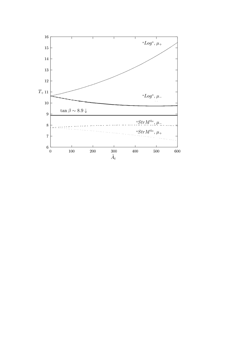
Figure 1: The $T_{+}$ model–independent lower bound on $\tan\beta$ in the top/stop–bottom/sbottom approximation and in the Supertrace approximation. Here: $M_{A}^{2}=m_{1}^{2}+m_{2}^{2}=(300\;{\rm GeV})^{2}$, $m_{3}^{2}=-(100\;{\rm GeV})^{2}$, $Q=m_{t}=175$ GeV, $M_{\rm SUSY}=630$ GeV, $\mu_{\pm}=\pm 100$ GeV and $Y_{t}=0.9$

2.3 Renormalization Group Evolution

In the minimal SUGRA model, the MSSM parameters [couplings and masses] are defined at the Unification scale with some unification conditions, and then are evolved down to the electroweak scale through Renormalization Group Equations (RGE). The RGE evolution is thus an important ingredient of mSUGRA, and more generally in any theory incorporating GUT unification. In the RGE’s of the MSSM, different levels of approximations are available as will be discussed later. In this section, we will write for completeness the RGE’s for the masses and couplings in the one–loop approximation, that we will need later when we will discuss the program SUSPECT.

In a next step, we will discuss some exact analytical solutions of the one–loop RG evolution equations of the Yukawa couplings. Solutions to these equations exist in the literature since many years [42] in the the limit where the top Yukawa coupling is assumed to dominate all the others. This limiting solution is relevant for small $\tan\beta$ values and remain numerically useful for $\tan\beta$ values up to 10 or so. Later on, various attempts were made to obtain general solutions, but still relying on some approximations, such as neglecting the U(1) coupling as compared to those of SU(3) and SU(2). However, even in this case, the solutions given where actually implicit [43] and not directly generalizable to include more than two Yukawa couplings ($Y_{t},Y_{b}$). Below, we will give the exact solutions with no approximation whatsoever. They are valid for any value of $Y_{t}$ and $Y_{b}$ and immediately generalizable to the full set of Yukawa couplings.

2.3.1 The one–loop RGE’s

In the following, we list the RGE’s for the MSSM parameters in the one–loop approximation. Although two–loop evolution equations for some parameters [such as the gauge and the Yukawa couplings] are available, for many purposes it is a rather good approximation to use only the one–loop equations [especially that it is much faster when implemented in numerical programs]. The list that we give below is ordered as in the program SUSPECT which will be discussed in section 3.2.

$\bullet$ Gauge Couplings [$g_{i}$ with $i=1,2,3$ and $n_{g}$ the generation number]:

$${\frac{dg_{i}}{dt}}={\frac{1}{32\pi^{2}}b_{i}g_{i}^{3}}\ \ {\rm with}\ \ b_{1}=-1-{\frac{10}{3}}n_{g}\ ,\ b_{2}=5-2n_{g}\ ,\ b_{3}=9-2n_{g}$$ (2.59)

$\bullet$ Yukawa Couplings [$i=1,2,3$ generations]:

$${\frac{dY_{u}^{i}}{dt}} = -{\frac{Y_{u}^{i}}{32\pi^{2}}}\bigg{[}{\sum_{k}3(Y_{u}^{k})^{2}+(Y_{d}^{i})^{2}}+3(Y_{u}^{i})^{2}-\bigg{(}{\frac{13}{9}}g_{1}^{2}+3g_{2}^{2}+\frac{16}{3}g_{3}^{2}\bigg{)}\bigg{]}$$ (2.60)

$${\frac{dY_{d}^{i}}{dt}} = -{\frac{Y_{d}^{i}}{32\pi^{2}}}\bigg{[}\sum_{k}\{3(Y_{d}^{k})^{2}+(Y_{l}^{k})^{2}\}+(Y_{u}^{i})^{2}+3(Y_{d}^{i})^{2}-\bigg{(}{\frac{7}{9}}g_{1}^{2}+3g_{2}^{2}+\frac{16}{3}g_{3}^{2}\bigg{)}\bigg{]}$$ (2.61)

$${\frac{dY_{l}^{i}}{dt}} = -{\frac{Y_{l}^{i}}{32\pi^{2}}}\bigg{[}\sum_{k}\{(Y_{l}^{k})^{2}+3(Y_{d}^{k})^{2}\}+3(Y_{l}^{i})^{2}-3(g_{1}^{2}+g_{2}^{2})\bigg{]}$$ (2.62)

$\bullet$ The $\mu$ term and the vacuum expectation values $v_{1}$, $v_{2}$ [$k=1,2,3$]:

$${\frac{d\mu}{dt}} = -{\frac{\mu}{32\pi^{2}}}\bigg{[}\sum_{k}3\{(Y_{u}^{k})^{2}+3(Y_{d}^{k})^{2}+(Y_{l}^{k})^{2}\}-(g_{1}^{2}+3g_{2}^{2})\bigg{]}$$ (2.63)

$${\frac{dv_{1}}{dt}} = {\frac{v_{1}}{32\pi^{2}}}\bigg{[}\sum_{k}\{3(Y_{d}^{k})^{2}+(Y_{l}^{k})^{2}\}-{\frac{3}{4}}\bigg{(}{\frac{1}{3}}g_{1}^{2}+g_{2}^{2}\bigg{)}\bigg{]}$$ (2.64)

$${\frac{dv_{2}}{dt}} = {\frac{v_{2}}{32\pi^{2}}}\bigg{[}{\sum_{k}3(Y_{u}^{k})^{2}}-{\frac{3}{4}}\bigg{(}{\frac{1}{3}}g_{1}^{2}+g_{2}^{2}\bigg{)}\bigg{]}$$ (2.65)

$\bullet$ The scalar Higgs masses and the parameter $B$ [$k=1,2,3$]:

$${\frac{dm^{2}_{H_{1}}}{dt}} = -{\frac{1}{16\pi^{2}}}\bigg{[}\sum_{k}\{3(Y_{d}^{k})^{2}P_{\tilde{d}}^{k}+(Y_{l}^{k})^{2}P_{\tilde{l}}^{k}\}-{\frac{1}{2}}g_{1}^{2}{\rm Tr}(Ym^{2})-(g_{1}^{2}M_{1}^{2}+3g_{2}^{2}M_{2}^{2})\bigg{]}$$ (2.66)

$${\frac{dm^{2}_{H_{2}}}{dt}} = -{\frac{1}{16\pi^{2}}}\bigg{[}{\sum_{k}3(Y_{u}^{k})^{2}P_{\tilde{u}}^{k}}+{\frac{1}{2}}g_{1}^{2}{\rm Tr}(Ym^{2})-(g_{1}^{2}M_{1}^{2}+3g_{2}^{2}M_{2}^{2})\bigg{]}$$ (2.67)

$${\frac{dB}{dt}} = -{\frac{1}{16\pi^{2}}}\bigg{[}\sum_{k}\{3A_{u}^{k}(Y_{u}^{k})^{2}+3A_{d}^{k}(Y_{d}^{k})^{2}+A_{d}^{k}(Y_{l}^{k})^{2}\}-(g_{1}^{2}M_{1}+3g_{2}^{2}M_{2})\bigg{]}$$ (2.68)

$\bullet$ The trilinear $A$ couplings $[i,k=1,2,3$]:

$${\frac{dA_{u}^{i}}{dt}} = -{\frac{1}{32\pi^{2}}}\bigg{[}6A_{u}^{i}(Y_{u}^{i})^{2}+2A_{d}^{i}(Y_{d}^{i})^{2}+6{\sum_{k}A_{u}^{k}(Y_{u}^{k})^{2}}$$ (2.69)

$$\hskip 39.83368pt-\bigg{(}{\frac{26}{9}}g_{1}^{2}M_{1}+6g_{2}^{2}M_{2}+{\frac{32}{3}}g_{3}^{2}M_{3}\bigg{)}\bigg{]}$$

$${\frac{dA_{d}^{i}}{dt}} = -{\frac{1}{32\pi^{2}}}\bigg{[}6A_{d}^{i}(Y_{d}^{i})^{2}+2A_{u}^{i}(Y_{u}^{i})^{2}+2\sum_{k}\{A_{l}^{k}(Y_{l}^{k})^{2}+3A_{d}^{k}(Y_{d}^{k})^{2}\}$$ (2.70)

$$\hskip 39.83368pt-\bigg{(}{\frac{14}{9}}g_{1}^{2}M_{1}+6g_{2}^{2}M_{2}+{\frac{32}{3}}g_{3}^{2}M_{3}\bigg{)}\bigg{]}$$

$${\frac{dA_{l}^{i}}{dt}} = -{\frac{1}{32\pi^{2}}}\bigg{[}6A_{l}^{i}(Y_{l}^{i})^{2}+2\sum_{k}\{A_{l}^{k}(Y_{l}^{k})^{2}+3A_{d}^{k}(Y_{d}^{k})^{2}\}-6(g_{1}^{2}M_{1}+g_{2}^{2}M_{2})\bigg{]}$$ (2.71)

$\bullet$ The scalar fermion masses [with $P^{k}_{\tilde{u},\tilde{d},\tilde{l}}\equiv m^{2}_{H_{2},H_{1},H_{2}}+m^{2}_{{\tilde{Q}}_{k},{\tilde{Q}}_{k},{\tilde{L}}_{k}}+m^{2}_{\tilde{u}_{k},\tilde{d}_{k},\tilde{l}_{k}}+(A^{k}_{u,d,l})^{2}$]

$${\frac{dm^{2}_{{\tilde{l}}_{R_{i}}}}{dt}} = -{\frac{1}{16\pi^{2}}}\bigg{[}2(Y_{l}^{i})^{2}P_{\tilde{l}}^{i}+g_{1}^{2}{\rm Tr}(Ym^{2})-4g_{1}^{2}M_{1}^{2}\bigg{]}$$ (2.72)

$${\frac{dm^{2}_{{\tilde{L}}_{i}}}{dt}} = -{\frac{1}{16\pi^{2}}}\bigg{[}(Y_{l}^{i})^{2}P_{\tilde{l}}^{i}-{\frac{1}{2}}g_{1}^{2}{\rm Tr}(Ym^{2})-(g_{1}^{2}M_{1}^{2}+3g_{2}^{2}M_{2}^{2})\bigg{]}$$ (2.73)

$${\frac{dm^{2}_{{\tilde{d}}_{R_{i}}}}{dt}} = -{\frac{1}{16\pi^{2}}}\bigg{[}2(Y_{d}^{i})^{2}P_{\tilde{d}}^{i}+{\frac{1}{3}}g_{1}^{2}{\rm Tr}(Ym^{2})-\bigg{(}{\frac{4}{9}}g_{1}^{2}M_{1}^{2}+{\frac{16}{3}}g_{3}^{2}M_{3}^{2}\bigg{)}\bigg{]}$$ (2.74)

$${\frac{dm^{2}_{{\tilde{u}}_{R_{i}}}}{dt}} = -{\frac{1}{16\pi^{2}}}\bigg{[}2(Y_{u}^{i})^{2}P_{\tilde{u}}^{i}-{\frac{2}{3}}g_{1}^{2}{\rm Tr}(Ym^{2})-\bigg{(}{\frac{16}{9}}g_{1}^{2}M_{1}^{2}+{\frac{16}{3}}g_{3}^{2}M_{3}^{2}\bigg{)}\bigg{]}$$ (2.75)

$${\frac{dm^{2}_{{\tilde{Q}}_{i}}}{dt}} = -{\frac{1}{16\pi^{2}}}\bigg{[}(Y_{u}^{i})^{2}P_{\tilde{u}}^{i}+(Y_{d}^{i})^{2}P_{\tilde{d}}^{i}+{\frac{1}{6}}g_{1}^{2}{\rm Tr}(Ym^{2})$$ (2.76)

$$\hskip 39.83368pt-\bigg{(}{\frac{1}{9}}g_{1}^{2}M_{1}^{2}+3g_{2}^{2}M_{2}^{2}+{\frac{16}{3}}g_{3}^{2}M_{3}^{2}\bigg{)}\bigg{]}$$

$\bullet$ The gaugino masses [$i=1,2,3$ and the $b_{i}$ are given above]

$${\frac{dM_{i}}{dt}}={\frac{1}{16\pi^{2}}M_{i}b_{i}g_{i}^{2}}$$ (2.77)

A few remarks are in order, here:

$(i)$ The evolution parameter $t$ is defined by $t={\rm Log}(M_{U}^{2}/Q^{2})$; this is different from the one used in the RGE’s of the program SUSPECT, where $t=1/2{\rm Log}(Q^{2}/M_{U}^{2})$. $(ii)$ Tr$(Ym^{2})$ is the isospin pondered sum of the squared soft masses of the scalar fermions; in the case of universal soft masses, the trace vanishes at any scale due to anomaly cancellation. $(iii)$ The RGE’s for the gaugino masses and the gauge couplings are related and from eqs. (2.59) and (2.77), one can easily see that $d/dt(M_{i}/g_{i}^{2})=0$.

2.3.2 Exact solutions for the Yukawa coupling RGE’s

We are interested here in eqs. (2.60–2.62). They have the nice feature of being completely decoupled from the rest of the system, especially from the gauge couplings whose running is determined a priori via eq. (2.59). [This is no more true at two–loop order where the gauge and Yukawa equations become interwound.] When all Yukawa couplings except $Y_{t}$ are neglected, eqs. (2.61) and (2.62) become trivial while eq. (2.60) becomes of the Bernoulli type in the variable $y_{t}\equiv Y_{t}^{2}$

$$\frac{d}{dt}y_{t}=f_{1}(t)y_{t}+by_{t}^{2}$$ (2.78)

where

$$f_{1}(t)=\frac{1}{16\pi^{2}}(\frac{16}{3}g_{3}^{2}+3g_{2}^{2}+\frac{13}{9}g_{1}^{2})\ \ ,\ \ b=-\frac{6}{16\pi^{2}}$$ (2.79)

and is easily solved to give [44, 42]

$$y_{t}(t)=\frac{y^{0}E(t)}{1-by^{0}\int_{0}^{t}E(t^{\prime})dt^{\prime}}$$ (2.80)

where

$$E(t)=e^{\int_{0}^{t}f_{1}(t^{\prime})dt^{\prime}}\ \ {\rm and}\ \ y^{0}=Y_{t}^{2}(t=0)$$ (2.81)

In the more general case where both $Y_{t}$ and $Y_{b}$ are kept in the game, but neglecting all other Yukawa couplings, eqs. (2.60,2.61) become after the change of variable, $y_{t}\equiv Y_{t}^{2},y_{b}\equiv Y_{b}^{2}$

$$\frac{d}{dt}y_{t} = f_{1}(t)y_{t}+ay_{b}y_{t}+by_{t}^{2}$$

$$\frac{d}{dt}y_{b} = f_{2}(t)y_{b}+ay_{b}y_{t}+by_{b}^{2}$$ (2.82)

where $f_{1}(t)$ and $b$ are given in eqs. (2.79) and

$$f_{2}(t)=\frac{1}{16\pi^{2}}(\frac{16}{3}g_{3}^{2}+3g_{2}^{2}+\frac{7}{9}g_{1}^{2})\ \ ,\ \ a=-\frac{1}{16\pi^{2}}$$ (2.83)

As far as we know, the system eqs. (2.82) is not treated in standard text books, and although it looks at first sight simple, we could not find a systematic way of relating it to a standard form. It is also relatively easy to solve the system up to first order in $Y_{b}$ in the region $Y_{t}\gg Y_{b}$ [4]. This is already an improvement of the known solutions with $Y_{b}\sim 0$. It extends the numerical validity much further than $\tan\beta\simeq 10$. More importantly, this approximate solution gave us a hint of the structure of the exact solution which was then found by sheer guess [4]:

$$y_{t}=\frac{y_{t}^{0}E_{12}(t)}{1-by_{t}^{0}\int_{0}^{t}E_{12}(t^{\prime})dt^{\prime}}$$ (2.84)

$$y_{b}=\frac{y_{b}^{0}E_{21}(t)}{1-by_{b}^{0}\int_{0}^{t}E_{21}(t^{\prime})dt^{\prime}}$$ (2.85)

where

$$E_{12}(t)=\frac{E_{1}(t)}{(1-by_{b}^{0}\int_{0}^{t}E_{21}(t^{\prime})dt^{\prime})^{a/b}}$$ (2.86)

$$E_{21}(t)=\frac{E_{2}(t)}{(1-by_{t}^{0}\int_{0}^{t}E_{12}(t^{\prime})dt^{\prime})^{a/b}}$$ (2.87)

$$E_{i}=e^{\int_{0}^{t}f_{i}(t^{\prime})dt^{\prime}}\;\;\;i=1,2$$ (2.88)

and $y_{t}^{0}\equiv Y_{t}^{2}(t=0),y_{b}^{0}\equiv Y_{b}^{2}(t=0)$ are arbitrary initial conditions. The solutions eqs. (2.84,2.85) are exact for any value of $\tan\beta$. They resemble formally eq. (2.80) of which they are a generalization. One should note however the important difference, namely that due to eqs. (2.86,2.87), the general solutions for $y_{t}$ and $y_{b}$ are actually continued integrated fractions. Indeed eqs. (2.86,2.87) give an implicit definition of $E_{12}(t)$ and $E_{21}(t)$, the first being defined in terms of the second and vice-versa. One could still write $E_{12}(t)$ in an explicit though infinite series form:

$$E_{12}(t)=\frac{E_{1}(t)}{(1-by_{b}^{0}\large{\int_{0}^{t}}\frac{E_{2}(t_{1})dt_{1}}{(1-by_{t}^{0}\int_{0}^{t_{1}}\frac{E_{1}(t_{2})dt_{2}}{(1-by_{b}^{0}\int_{0}^{t_{2}}\frac{E_{2}(t_{3})dt_{3}}{(1-by_{t}^{0}\int_{0}^{t_{3}}\cdots)^{a/b}})^{a/b}})^{a/b}})^{a/b}}$$ (2.89)

and similarly for $E_{21}(t)$ with the substitution $1\leftrightarrow 2,y_{t}^{0}\leftrightarrow y_{b}^{0}$. We will see later on that both forms for $E_{ij}$ are useful. In any case, we should stress here that the solutions for $y_{t},y_{b}$ are themselves explicit.

What do we gain from these exact analytical solutions?

$(i)$ First of all one can prove rigorously the convergence of the infinite series $E_{ij}(t)$ and determine explicitly the convergence criteria [4]. This implies that, for practical purposes, keeping only the first iteration of the $E_{ij}(t)$ series is numerically a very good approximation [within the convergence region]. We give in Table 1 a numerical comparison versus a Runge-Kutta method.

$(ii)$  The large $\tan\beta$ region is treated exactly and one can follow precisely the various features of the running of the Yukawa couplings in this regime.

$(iii)$ The fact that the coefficients of the quadratic parts of eqs. (2.82) are equal and that there are only two non-zero Yukawa couplings is actually unessential in finding the general solutions in the present form. This form generalizes straightforwardly for an exact solution of eqs. (2.60–2.62) which will be given elsewhere [4], and would thus be of relevance in the case of bottom–tau Yukawa coupling unification scenarios [34].

$(iv)$ Finally, one can control analytically the acceptable regions for the initial conditions $y_{b}^{0},y_{t}^{0}$. This is related to the necessity of avoiding Landau poles and more generally of requiring $y_{t},y_{b}$ to remain positive throughout the evolution, being the squares of $Y_{t},Y_{b}$. This is of relevance if one wants to run the quantities between two low-energy scales choosing some initial conditions at one of these scales without referring explicitly to the initial values at the unification scale $M_{U}$. [Such a possibility is being implemented in the fortran code SUSPECT, see section 3.2].

$\tan\beta$	$Y_{b}(t=0)$	$Y_{t}(t=0)$	$Y_{b}(t)$	$Y_{b}(t)$	$Y_{t}(t)$	$Y_{t}(t)$
			“exact”	Runge-Kutta	“exact”	Runge-Kutta
2	0.0387453	1.13007	0.0145059	0.0145050	0.775788	0.775974
10	0.174138	1.01581	0.0630978	0.0631052	0.54263	0.542743
50	0.866544	1.01097	0.435682	0.439526	0.585453	0.590258

Table 1: Numerical comparison of the exact one–loop solution, truncated to the first iteration, with the Runge–Kutta RG evolution, obtained with only a one step evolution over 10 orders of magnitude.

3. The Physical Parameters

3.1 Particle masses and couplings

3.1.1 Mass matrices and couplings

In this section, we discuss the general features of the chargino/neutralino, sfermion and Higgs boson sectors to set the conventions and the notations which will be used further on.

a) The chargino/neutralino sector

The general chargino mass matrix depends on the parameters $M_{2},\mu$ and $\mbox{tan}\beta$ [22, 45]

$${\cal M}_{C}=\left[\begin{array}[]{cc}M_{2}&\sqrt{2}M_{W}\sin\beta\\ \sqrt{2}M_{W}\cos\beta&\mu\end{array}\right]$$ (3.3)

is diagonalized by two real matrices $U$ and $V$,

$$U^{*}{\cal M}_{C}V^{-1}\ \ \rightarrow\ \ U={\cal O}_{-}\ {\rm and}\ \ V=\left\{\begin{array}[]{cc}{\cal O}_{+}&{\rm if\ det}{\cal M}_{C}\geq 0\\ \sigma_{3}{\cal O}_{+}&{\rm if\ det}{\cal M}_{C}<0\end{array}\right.$$ (3.6)

where the $\sigma_{3}$ matrix and the ${\cal O}_{\pm}$ matrices are given by [with the appropriate signs depending on the values of $M_{2}$, $\mu$, and $\tan\beta$]

$${\sigma_{3}}=\left[\begin{array}[]{cc}+1&0\\ 0&-1\end{array}\right]\ \ ,\ \ {\cal O}_{\pm}=\left[\begin{array}[]{cc}\cos\theta_{\pm}&\sin\theta_{\pm}\\ -\sin\theta_{\pm}&\cos\theta_{\pm}\end{array}\right]$$ (3.11)

with

$$\tan 2\theta_{-} = \frac{2\sqrt{2}M_{W}(M_{2}\cos\beta+\mu\sin\beta)}{M_{2}^{2}-\mu^{2}-2M_{W}^{2}\cos\beta}$$

$$\tan 2\theta_{+} = \frac{2\sqrt{2}M_{W}(M_{2}\sin\beta+\mu\cos\beta)}{M_{2}^{2}-\mu^{2}+2M_{W}^{2}\cos\beta}$$ (3.12)

This leads to the two chargino masses,

$$m_{\chi_{1,2}^{+}}= \frac{1}{\sqrt{2}}\left[M_{2}^{2}+\mu^{2}+2M_{W}^{2}\right.$$

$$\left.\mp\left\{(M_{2}^{2}-\mu^{2})^{2}+4M_{W}^{4}\cos^{2}2\beta+4M_{W}^{2}(M^{2}_{2}+\mu^{2}+2M_{2}\mu\sin 2\beta)\right\}^{\frac{1}{2}}\right]^{\frac{1}{2}}$$

In the limit $|\mu|\gg M_{2},M_{Z}$, the masses of the two charginos reduce to $[\epsilon_{\mu}\equiv{\rm sign}(\mu)$]

$$m_{\chi_{1}^{+}} \simeq M_{2}-\frac{M_{W}^{2}}{\mu^{2}}\left(M_{2}+\mu\sin 2\beta\right)$$

$$m_{\chi_{2}^{+}} \simeq |\mu|+\frac{M_{W}^{2}}{\mu^{2}}\epsilon_{\mu}\left(M_{2}\sin 2\beta+\mu\right)$$ (3.14)

For $|\mu|\rightarrow\infty$, the lightest chargino corresponds to a pure wino state with $m_{\chi_{1}^{+}}\simeq M_{2}$, while the heavier chargino corresponds to a pure higgsino state with $m_{\chi_{2}^{+}}=|\mu|$.

In the case of the neutralinos, the four–dimensional neutralino mass matrix [22] depends on the same two mass parameters $\mu$ and $M_{2}$, if the GUT relation $M_{1}=\frac{5}{3}\tan^{2}\theta_{W}$ $M_{2}\simeq\frac{1}{2}M_{2}$ is used. In the $(-i\tilde{B},-i\tilde{W}_{3},\tilde{H}^{0}_{1},$ $\tilde{H}^{0}_{2})$ basis, it has the form [$s_{W}^{2}=1-c_{W}^{2}\equiv\sin^{2}\theta_{W}$]

$${\cal M}_{N}=\left[\begin{array}[]{cccc}M_{1}&0&-M_{Z}s_{W}\cos\beta&M_{Z}s_{W}\sin\beta\\ 0&M_{2}&M_{Z}c_{W}\cos\beta&-M_{Z}c_{W}\sin\beta\\ -M_{Z}s_{W}\cos\beta&M_{Z}c_{W}\cos\beta&0&-\mu\\ M_{Z}s_{W}\sin\beta&-M_{Z}c_{W}\sin\beta&-\mu&0\end{array}\right]$$ (3.19)

It can be diagonalized analytically [46] by a single real matrix $Z$; the [positive] masses of the neutralino states $m_{\chi_{i}^{0}}$ have complicated expressions which will not be given here. In the limit of large $|\mu|$ values, the masses of the neutralino states however simplify to

$$m_{\chi_{1}^{0}} \simeq M_{1}-\frac{M_{Z}^{2}}{\mu^{2}}\left(M_{1}+\mu\sin 2\beta\right)s_{W}^{2}$$

$$m_{\chi_{2}^{0}} \simeq M_{2}-\frac{M_{Z}^{2}}{\mu^{2}}\left(M_{2}+\mu\sin 2\beta\right)c_{W}^{2}$$

$$m_{\chi_{3}^{0}} \simeq |\mu|+\frac{1}{2}\frac{M_{Z}^{2}}{\mu^{2}}\epsilon_{\mu}(1-\sin 2\beta)\left(\mu+M_{2}s_{W}^{2}+M_{1}c_{W}^{2}\right)$$

$$m_{\chi_{4}^{0}} \simeq |\mu|+\frac{1}{2}\frac{M_{Z}^{2}}{\mu^{2}}\epsilon_{\mu}(1+\sin 2\beta)\left(\mu-M_{2}s_{W}^{2}-M_{1}c_{W}^{2}\right)$$ (3.20)

Again, for $|\mu|\rightarrow\infty$, two neutralinos are pure gaugino states with masses $m_{\chi_{1}^{0}}\simeq M_{1}$ , $m_{\chi_{2}^{0}}=M_{2}$, while the two others are pure higgsino states, with masses $m_{\chi_{3}^{0}}\simeq m_{\chi_{4}^{0}}\simeq|\mu|$.

b) The sfermion sector

Assuming a universal scalar mass $m_{0}$ and gaugino mass $m_{1/2}$ at the GUT scale, one obtains relatively simple expressions for the left– and right–handed sfermion masses when performing the RGE evolution to the weak scale at one–loop order, if the the Yukawa couplings in the RGE’s are neglected [for third generation squarks this is a poor approximation since these couplings can be large; in this case numerical analyses are needed as will be discussed later]. One has:

$$m_{\tilde{f}_{L,R}}^{2}=m_{0}^{2}+\sum_{i=1}^{3}F_{i}(f)m^{2}_{1/2}\pm(I^{3}_{f}-e_{f}s_{W}^{2})M_{Z}^{2}\cos 2\beta$$ (3.21)

$I_{f}^{3}$ and $e_{{f}}$ are the weak isospin and the electric charge of the sfermion and $F_{i}$ are the RGE coefficients for the three gauge couplings at the scale $Q\sim M_{Z}$, given by

$$F_{i}=\frac{c_{i}(f)}{b_{i}}\left[1-\left(1-\frac{\alpha_{U}}{4\pi}b_{i}{\rm Log}\frac{Q^{2}}{M_{U}^{2}}\right)^{-2}\right]$$ (3.22)

The coefficients $b_{i}$, assuming that all the MSSM particle spectrum contributes to the evolution from $Q$ to the GUT scale $M_{G}$, are given by: $b_{1}=33/5,b_{2}=1,b_{3}=-3$. The coefficients $c(\tilde{f})=(c_{1},c_{2},c_{3})(\tilde{f})$ depend on the hypercharge and color of the sfermions

$$c(\tilde{L})=\left(\begin{array}[]{c}{3\over 10}\\ {3\over 2}\\ 0\end{array}\right),c(\tilde{l}_{R})=\left(\begin{array}[]{c}{6\over 5}\\ 0\\ 0\end{array}\right),c(\tilde{Q})=\left(\begin{array}[]{c}{1\over 30}\\ {3\over 2}\\ {8\over 3}\end{array}\right),c(\tilde{u}_{R})=\left(\begin{array}[]{c}{8\over 15}\\ 0\\ {8\over 3}\end{array}\right),c(\tilde{d}_{R})=\left(\begin{array}[]{c}{2\over 15}\\ 0\\ {8\over 3}\end{array}\right)$$ (3.38)

With the input gauge coupling constants at the scale of the $Z$ boson mass $\alpha_{1}(M_{Z})\simeq 0.01,\alpha_{2}(M_{Z})\simeq 0.033$ and $\alpha_{3}(M_{Z})\simeq 0.118$, one obtains $M_{U}\sim 1.9\times 10^{16}$ GeV for the GUT scale and $\alpha_{U}=0.041$ for the coupling constant $\alpha_{U}$. Using these values, one obtains for the left– and right–handed sfermion masses

$$m^{2}_{\tilde{u}_{L}} = m_{0}^{2}+6.28m^{2}_{1/2}+0.35M_{Z}^{2}\cos 2\beta$$

$$m^{2}_{\tilde{d}_{L}} = m_{0}^{2}+6.28m^{2}_{1/2}-0.42M_{Z}^{2}\cos 2\beta$$

$$m^{2}_{\tilde{u}_{R}} = m_{0}^{2}+5.87m^{2}_{1/2}+0.16M_{Z}^{2}\cos 2\beta$$

$$m^{2}_{\tilde{d}_{R}} = m_{0}^{2}+5.82m^{2}_{1/2}-0.08M_{Z}^{2}\cos 2\beta$$

$$m^{2}_{\tilde{\nu}_{L}} = m_{0}^{2}+0.52m^{2}_{1/2}+0.50M_{Z}^{2}\cos 2\beta$$

$$m^{2}_{\tilde{e}_{L}} = m_{0}^{2}+0.52m^{2}_{1/2}-0.27M_{Z}^{2}\cos 2\beta$$

$$m^{2}_{\tilde{e}_{R}} = m_{0}^{2}+0.15m^{2}_{1/2}-0.23M_{Z}^{2}\cos 2\beta$$ (3.39)

In the case of the third generation sparticles, left– and right–handed sfermions will mix [47]; for a given sfermion $\tilde{f}=\tilde{t},\tilde{b}$ and $\tilde{\tau}$, the mass matrices which determine the mixing are given by

$$M_{\tilde{f}}^{2}\ =\ \left[\begin{array}[]{cc}m_{\tilde{f}_{L}}^{2}+m_{f}^{2}&m_{f}(A_{f}-\mu r_{f})\\ m_{f}(A_{f}-\mu r_{f})&m_{\tilde{f}_{R}}^{2}+m_{f}^{2}\end{array}\right]$$ (3.42)

where the sfermion masses $m_{\tilde{f}_{L,R}}$ are given above, $m_{f}$ are the masses of the partner fermions and $r_{b}=r_{\tau}=1/r_{t}=\mbox{tan}\beta$. These matrices are diagonalized by orthogonal matrices; the mixing angles $\theta_{f}$ and the squark eigenstate masses are given by

$$\sin 2\theta_{f}=\frac{2m_{f}(A_{f}-\mu r_{f})}{m_{\tilde{f}_{1}}^{2}-m_{\tilde{f}_{2}}^{2}}\ \ ,\ \ \cos 2\theta_{f}=\frac{m_{\tilde{f}_{L}}^{2}-m_{\tilde{f}_{R}}^{2}}{m_{\tilde{f}_{1}}^{2}-m_{\tilde{f}_{2}}^{2}}\hskip 22.76228pt$$ (3.43)

$$m_{\tilde{f}_{1,2}}^{2}=m_{f}^{2}+\frac{1}{2}\left[m_{\tilde{f}_{L}}^{2}+m_{\tilde{f}_{R}}^{2}\mp\sqrt{(m_{\tilde{f}_{L}}^{2}-m_{\tilde{f}_{R}}^{2})^{2}+4m_{f}^{2}(A_{f}-\mu r_{f})^{2}}\right]$$ (3.44)

Due to the large value of $m_{t}$, the mixing is particularly strong in the stop sector. This generates a large splitting between the masses of the two stop eigenstates, possibly leading to a lightest top squark much lighter than the other squarks and even the top quark.

c) The Higgs sector

We come now to a description of our parameterization of the MSSM Higgs sector [23]. Besides the four masses, $M_{h},M_{H},M_{A}$ and $M_{H^{\pm}}$, the Higgs sector is described at the tree level by two additional parameters, $\mbox{tan}\beta$ and a mixing angle $\alpha$ in the CP–even Higgs sector. Due to SUSY constraints as discussed before, only two of them are independent and the two inputs are in general taken to be $\mbox{tan}\beta$ and $M_{A}$. Radiative corrections, the leading part of which grow as the fourth power of the top mass and logarithmically with the common squark mass [48, 49], change significantly the relations between masses and couplings and shift the mass of the lightest $h$ boson upwards. These radiative corrections are very important and should therefore be included in any analysis. Here we will, however, only discuss the leading part of this correction which in the simplest case can be parameterized in terms of the quantity [48]

$$\epsilon=\frac{3G_{F}}{\sqrt{2}\pi^{2}}\frac{m_{t}^{4}}{\sin^{2}\beta}{\rm Log}\left(1+\frac{m_{\tilde{q}}^{2}}{m_{t}^{2}}\right)\ .$$ (3.45)

The CP–even Higgs boson masses are then given in terms of the pseudoscalar mass $M_{A}$ and $\mbox{tan}\beta$, and the charged Higgs boson mass in terms of $M_{A}$, are given by

$$M_{h,H}^{2}=\frac{1}{2}\Bigg{[}M_{A}^{2}+M_{Z}^{2}+\epsilon\mp\sqrt{(M_{A}^{2}+M_{Z}^{2}+\epsilon)^{2}-4M_{A}^{2}M_{Z}^{2}\cos^{2}2\beta-4\epsilon(M_{A}^{2}\sin^{2}\beta+M_{Z}^{2}\cos^{2}\beta)}\Bigg{]}$$

$$M_{H^{\pm}}^{2}=M_{A}+M_{W}^{2}\hskip 170.71652pt$$ (3.46)

The mixing angle $\alpha$ reads in terms of $M_{A}$ and $\mbox{tan}\beta$

$$\tan 2\alpha = \tan 2\beta\frac{M_{A}^{2}+M_{Z}^{2}}{M_{A}^{2}-M_{Z}^{2}+\epsilon/\cos 2\beta}\ ,\hskip 28.45274pt-\frac{\pi}{2}\leq\alpha\leq 0\ .$$ (3.47)

Once $\mbox{tan}\beta$ and $M_{A}$ are chosen and the leading radiative correction is included in $\alpha$, all the couplings of the Higgs bosons to fermions, gauge bosons and Higgs bosons are fixed. However, in the trilinear MSSM Higgs boson couplings, there are also large radiative corrections which are not entirely mapped into the angle $\alpha$, but the leading part can also be expressed in terms of the leading correction $\epsilon$ [50].

$\hskip 28.45274pt\Phi\hskip 28.45274pt$	$g_{\Phi\bar{u}u}$	$g_{\Phi\bar{d}d}$	$g_{\Phi VV}$	$g_{\Phi VA}$
$h$	$\;\cos\alpha/\sin\beta\;$	$\;-\sin\alpha/\cos\beta\;$	$\sin(\beta-\alpha)$	$\cos(\beta-\alpha)$
$H$	$\;\sin\alpha/\sin\beta\;$	$\;\cos\alpha/\cos\beta\;$	$\cos(\beta-\alpha)$	$-\sin(\beta-\alpha)$
$A$	$\;1/\mbox{tan}\beta\;$	$\;\mbox{tan}\beta\;$	$0$	$0$

Table 2: Higgs boson couplings in the MSSM to fermions and gauge bosons relative to the SM Higgs couplings, and coupling to Higgs and gauge bosons.

The couplings of the charged Higgs boson to down (up) type fermions are (inversely) proportional to $\mbox{tan}\beta$, as in the case of the pseudoscalar Higgs boson. For the CP–even Higgs bosons, the couplings to down (up) type fermions are enhanced (suppressed) compared to the SM Higgs couplings [$\mbox{tan}\beta>1$]; the couplings to gauge bosons are suppressed by $\sin/\cos(\beta-\alpha)$ factors. $A$ has no tree level couplings to gauge bosons. Note also that while the couplings of the $h$ and $H$ bosons to $ZA$ and $W^{+}H^{-}$ pairs are proportional to $\cos$ and $\sin(\beta-\alpha)$ respectively, the $W^{+}H^{-}A$ coupling is not suppressed by these factors. The couplings of the MSSM neutral Higgs bosons to fermions and gauge bosons [normalized to the SM Higgs coupling $g_{H_{\rm SM}ff}=(\sqrt{2}G_{F})^{1/2}m_{f}$ and $g_{H_{\rm SM}VV}=2(\sqrt{2}G_{F})^{1/2}M_{V}^{2}$] and to gauge and Higgs bosons [normalized to $(\sqrt{2}G_{F})^{1/2}/M_{Z}(p_{\Phi}+p_{A})_{\mu}$ with $p_{\Phi}$ and $p_{A}$ the Higgs bosons 4–momenta] are given in Table 2.

Let us turn now to the $h$ boson couplings to stop squarks which will be a very important ingredient for the discussion of the next section 4. Normalized to $2M_{Z}^{2}(\sqrt{2}G_{F})^{1/2}$, they are given in the decoupling limit $M_{A}\gg M_{Z}$, by

$$g_{h\tilde{t}_{1}\tilde{t}_{1}} = -\cos 2\beta\left[\frac{1}{2}\cos^{2}\theta_{\tilde{t}}-\frac{2}{3}s^{2}_{W}\cos 2\theta_{\tilde{t}}\right]-\frac{m_{t}^{2}}{M_{Z}^{2}}+\frac{1}{2}\sin 2\theta_{\tilde{t}}\frac{m_{t}\tilde{A}_{t}}{M_{Z}^{2}}$$

$$g_{h\tilde{t}_{2}\tilde{t}_{2}} = -\cos 2\beta\left[\frac{1}{2}\sin^{2}\theta_{\tilde{t}}-\frac{2}{3}s_{W}^{2}\cos 2\theta_{\tilde{t}}\right]-\frac{m_{t}^{2}}{M_{Z}^{2}}-\frac{1}{2}\sin 2\theta_{\tilde{t}}\frac{m_{t}\tilde{A}_{t}}{M_{Z}^{2}}$$ (3.48)

and involve components which are proportional to $\tilde{A}_{t}=A_{t}-\mu/\tan\beta$. For large values of the parameter $\tilde{A}_{t}$ which incidentally make the $\tilde{t}$ mixing angle maximal, $|\sin 2\theta_{\tilde{t}}|\simeq 1$, the last components can strongly enhance the $g_{h\tilde{t}\tilde{t}}$ couplings and make them larger than the top quark coupling of the $h$ boson, $g_{htt}\propto m_{t}/M_{Z}$. The couplings of the heavy $H$ boson to stops involve also components which can be large; in the case of the lightest stops, the coupling reads in the decoupling limit:

$$g_{H\tilde{t}_{1}\tilde{t}_{1}}=\sin 2\beta\left[\frac{1}{2}\cos^{2}\theta_{\tilde{t}}-\frac{2}{3}s^{2}_{W}\cos 2\theta_{\tilde{t}}\right]-\frac{m_{t}^{2}}{M_{Z}^{2}}\frac{1}{\mbox{tan}\beta}+\frac{1}{2}\sin 2\theta_{\tilde{t}}\frac{m_{t}}{M_{Z}^{2}}(\frac{A_{t}}{\mbox{tan}\beta}+\mu)$$ (3.49)

For large $\mbox{tan}\beta$ values, the $m_{t}^{2}$ and the $A_{t}$ components are suppressed; only the component proportional to $\mu$ is untouched. The pseudoscalar $A$ couples only to $\tilde{t}_{1}\tilde{t}_{2}$ pairs because of CP–invariance, the coupling is given by:

$$g_{A\tilde{t}_{1}\tilde{t}_{2}} = \frac{1}{2}\frac{m_{t}}{M_{Z}^{2}}(A_{t}/\mbox{tan}\beta-\mu)$$ (3.50)

In the maximal mixing case, $|\sin 2\theta_{\tilde{t}}|\simeq 1$, this is also the main component of the $H$ boson coupling to $\tilde{t}_{1}\tilde{t}_{2}$ pairs except that the sign of $\mu$ is reversed.

Finally, let us exhibit the couplings of the $h$ boson to sneutrinos and the lightest neutralinos that we will need in section 4.2. For sneutrinos, the couplings is just given in eq. (3.48) and setting the fermion mass and the mixing angle to zero:

$$g_{h\tilde{\nu}\tilde{\nu}}=-\frac{1}{2}\cos 2\beta$$ (3.51)

For the normalized couplings of the $h$ boson to the LSP, one has

$$g_{h\chi_{1}^{0}\chi_{1}^{0}}=(Z_{12}-\tan\theta_{W}Z_{11})(\sin\beta Z_{14}-\cos\beta Z_{13})$$ (3.52)

with $Z$ is the matrix diagonalizing the neutralino mass matrix discussed above.

3.1.2 Inverting the chargino/neutralino spectrum

Once a few super–partners will be discovered at LEP/LHC, the next immediate task would be to reconstruct from the measured parameters, as precisely as possible, the structure of the soft–SUSY breaking Lagrangian. Although the relationship between physical parameters [mass eigenvalues, mixing angles and physical couplings] and e.g. the phenomenological MSSM Lagrangian is well established [21, 22, 23], it would be useful to invert such a relationship, namely to derive Lagrangian parameters directly from physical parameters. This is however especially non–trivial in the neutralino sector, which involves the $4\times 4$ mass matrix shown above to “de–diagonalize”.

Here, we illustrate a relatively simple scheme for such an analytic inversion [5] for most of the Lagrangian parameters of the phenomenological MSSM, in terms of a minimal set of appropriately chosen physical input parameters. In the pure gaugino sector, the algorithm gives for a given $\tan\beta$ the values of the $\mu$, $M_{1}$ and $M_{2}$ parameters in terms of three arbitrary input masses, chosen indifferently among four, namely either two chargino and one neutralino masses or two neutralino and one chargino masses.

Note that, in a more standard approach [i.e. from the Lagrangian to the physical parameters], one may obtain a similar information, e.g. by some systematic scanning of the whole parameter space. However, the advantage of having relatively simple [and thus fast] analytical expressions should be obvious, since in practice a complete scanning of the unconstrained MSSM parameters would be rather tedious and probably not particularly illuminating [for a recent detailed analysis, although in the more constrained mSUGRA scenario, see Ref. [51] for instance]. In addition, there are some subtleties in such a reconstruction, like the occurrence of possible discrete ambiguities which are most clearly seen via explicit inversion, as we shall illustrate.

Let us now sketch our general procedure to reconstruct the gaugino sector parameters; for more details we refer to Ref. [5]. First, one should fix a specific choice of input/output parameters and a simple starting point is to assume that $\tan\beta$ is an input i.e. that it has been extracted from elsewhere prior to gaugino reconstruction [see e.g. section 5.2]. Then, we consider two basic algorithms or “scenarii”, that we call $S_{1}$ and $S_{2}$.

Scenario $S_{1}$: here, the input masses are assumed to be the two chargino masses $m_{\chi^{\pm}_{1}}$ and $m_{\chi^{\pm}_{2}}$ and one (but any) neutralino mass $\pm m_{\chi_{i}^{0}}$. Then, the algorithm $S_{1}$ gives the parameters: $\mu$, $M_{2}$, $M_{1}$, plus the values of the three other neutralino masses $m_{\chi_{j}^{0}},(j\neq i)$. More precisely, when assuming that $\tan\beta$ and the two chargino masses are given, the basic equations giving $\mu$ and $M_{2}$ are simply obtained by inverting the chargino mass expressions eqs. (3.1.1 Mass matrices and couplings), obtaining

$$\mu^{2}=\frac{1}{2}(m^{2}_{\chi_{1}^{\pm}}+m^{2}_{\chi_{2}^{\pm}}-2M^{2}_{W}\pm[(m^{2}_{\chi_{1}^{\pm}}+m^{2}_{\chi_{2}^{\pm}}-2M^{2}_{W})^{2}-4(M^{2}_{W}\sin 2\beta\pm m_{\chi_{1}^{\pm}}m_{\chi_{2}^{\pm}})^{2}]^{1/2})$$

$$M_{2}=[m^{2}_{\chi_{1}^{\pm}}+m^{2}_{\chi_{2}^{\pm}}-2M^{2}_{W}-\mu^{2}]^{1/2}\hskip 142.26378pt$$ (3.53)

with the sign of $\mu$ determined from

$$M_{2}\;\mu=M^{2}_{W}\sin 2\beta\pm m_{\chi_{1}^{\pm}}m_{\chi_{2}^{\pm}}$$ (3.54)

Note that in eq. (3.1.2 Inverting the chargino/neutralino spectrum), the $\pm$ in front of the square root simply reflects the spurious $\mu^{2}\leftrightarrow M^{2}_{2}$ ambiguity, while the $\pm$ inside the square root or in eq.  (3.54) corresponds to a true ambiguity, i.e. when the expression under the root is positive (or zero) for both sign choice there are two possible solutions for ($\mu$, $M_{2}$). The occurrence of this twofold ambiguity crucially depends, obviously, on the mass values $m_{\chi_{1}^{\pm}}$, $m_{\chi_{2}^{\pm}}$ and $\tan\beta$, as will be illustrated. It is relatively easy to determine in which parameter domain one has either no solution, a unique or twofold solution.

Concerning the neutralino mass inversion, we note first that since we restrict ourselves to the case where $M_{1},M_{2}$ and $\mu$ are all real–valued, the neutralino mass matrix is symmetric and can be diagonalized through a similarity transformation, i.e.

$$PM_{N}P^{-1}=M_{N}^{\rm diagonal}$$ (3.55)

Now, rather than an analytically cumbersome inversion of the mass eigenvalue expressions, a simpler procedure is to start from the four basic invariants

$${\rm Tr}M\ ,\ \frac{1}{2}({\rm Tr}M)^{2}-\frac{1}{2}{\rm Tr}M^{2}\ ,\ \frac{1}{6}({\rm Tr}M)^{3}-\frac{1}{2}{\rm Tr}M\,{\rm Tr}M^{2}+\frac{1}{3}{\rm Tr}M^{3}\ ,\ {\rm Det}M$$ (3.56)

under similarity transformations. These invariants contain the complete information on the relationship between the mass eigenvalues and the initial parameters in the neutralino mass matrix, but do not favor any particular set of parameters. Thus, the system may be solved in many different ways depending on the choice of input/output one is interested in. In fact, the necessary and sufficient conditions for the existence of solutions to eq. (3.56) take the form

$$P_{23}^{2}+(\mu^{2}+M_{Z}^{2}-M_{1}M_{2}+(M_{1}+M_{2})S_{23}-S_{23}^{2})P_{23}$$

$$+\mu M_{Z}^{2}(c_{W}^{2}M_{1}+s_{W}^{2}M_{2})\sin 2\beta-\mu^{2}M_{1}M_{2}=0$$ (3.57)

$$(M_{1}+M_{2}-S_{23})P_{23}^{2}+(\mu^{2}(M_{1}+M_{2})+M_{Z}^{2}(c_{W}^{2}M_{1}+s_{W}^{2}M_{2}-\mu\sin 2\beta))P_{23}$$

$$+\mu(M_{Z}^{2}(c_{W}^{2}M_{1}+s_{W}^{2}M_{2})\sin 2\beta-\mu M_{1}M_{2})S_{23}=0$$ (3.58)

where $S_{23}=\tilde{m}_{\chi^{0}_{2}}+\tilde{m}_{\chi^{0}_{3}}$ and $P_{23}=\tilde{m}_{\chi^{0}_{2}}\tilde{m}_{\chi^{0}_{3}}$ [with similar equations for all possible combinations of two neutralino masses, ($\tilde{m}_{\chi^{0}_{i}}$, $\tilde{m}_{\chi^{0}_{j}}$)]. These equations constitute our basics to invert the neutralino sector. For instance, in scenario $S_{1}$ we can extract $M_{1}$ and the three physical masses $m_{\chi^{0}_{1}}$, $m_{\chi^{0}_{3}}$, $m_{\chi^{0}_{4}}$ as functions of the mass $m_{\chi^{0}_{2}}$, from any one of eqs. (3.57) or (3.58). Note that the mass $m_{\chi^{0}_{2}}$ plays the role of any neutralino mass to be given as input, i.e. there will be a relabeling of neutralino states depending on the values of the other parameters.

Scenario $S_{2}$: here, we assume that $\mu$ [alternatively $M_{2}$] is an input parameter together with two neutralino masses, say $m_{\chi^{0}_{2}}$ and $m_{\chi^{0}_{3}}$. Then, the quadratic system eqs. (3.57) and (3.58) gives $M_{2}$ and $M_{1}$. The key point is that it is relatively simple to merge these two basic algorithms, $S_{1}$ and $S_{2}$, to also obtain $\mu$, $M_{2}$, $M_{1}$ consistently from $m_{\chi^{\pm}_{1}}$, $m_{\chi^{0}_{2}}$, and $m_{\chi^{0}_{3}}$; for instance choosing an arbitrary initial guess value for $m_{\chi^{\pm}_{2}}$ [alternatively $M_{2}$], one simply has to use $S_{1}$ followed by $S_{2}$, eventually iterating until a consistent, i.e. convergent, set of values is obtained. In most practical cases, convergence is very fast after 2 or 3 iterations. This peculiar decomposition, with this choice of input/output masses is deliberately chosen as the one giving the most algebraically tractable inversion in the gaugino sector. It does not imply however, a strong particular prejudice on the chronology of discovery of the gauginos. The most likely situation where one would presumably first discover two neutralinos and only one chargino, is precisely tractable from the combined $S_{1}$ + $S_{2}$ algorithm as explained above. The price to pay however, is that scenario $S_{1}+S_{2}$ [with only one chargino mass input $m_{\chi^{\pm}_{1}}$, and without further model assumption] potentially gives more ambiguities than $S_{1}$ alone. The upshot is that up to four (at most) distinct solutions for ($\mu$, $M_{1}$, $M_{2}$) can occur for some $m_{\chi^{\pm}_{1}}$, $m_{\chi^{0}_{2}}$, $m_{\chi^{0}_{3}}$ input choices once all constraints are taken into account [including in particular our necessary sign convention $M_{2}>0$].

Let us illustrate with some representative plots the results of the inversion in the gaugino sector according to the algorithms $S_{1}$ and $S_{2}$. As it turns out, a number of general and interesting properties of the inversion can directly be seen irrespective of the precise values of the other parameters that have to be fixed, like $\tan\beta$ typically.

$(i)$ Two charginos plus one neutralino input

We first discuss the basic algorithm $S_{1}$ in Fig. 2, where to exhibit as much as possible the dependence on the physical inputs, we fixed only one chargino mass, say $m_{\chi^{\pm}_{1}}$, and varied the other mass $m_{\chi^{\pm}_{2}}$. Fig. 2 exhibits characteristics that are quite generic; there are three distinct zones as regards the existence, uniqueness, or possible ambiguities on the parameters $\mu$, $M_{2}$, $M_{1}$:

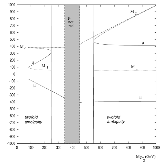
Figure 2: The parameters $\mu$, $M_{2}$ and $M_{1}$ as functions of $m_{\chi^{\pm}_{2}}$ for fixed $m_{\chi^{\pm}_{1}}=400$ GeV, $m_{\chi^{\pm}_{2}}=50$ GeV and $\tan\beta=2$.

a) The grey shaded region corresponds to $m_{\chi^{\pm}_{1}}^{2}+m_{\chi^{\pm}_{2}}^{2}<2M_{W}^{2}$ where there are no solutions for real $\mu$ that has to be rejected according to our basic assumptions; if one takes a smaller or larger $m_{\chi^{\pm}_{1}}$ value, this region around $m_{\chi^{\pm}_{1}}$ will be simply displaced accordingly. ${\it b)}$ In the left and right border zones are the regions of twofold ambiguities on $\mu$, $M_{2}$ as indicated. c) Finally the two bands in between zones a) and b) correspond to the region where eqs. (3.1.2 Inverting the chargino/neutralino spectrum) give a unique solution for $\mu$ and $M_{2}$; note that those bands are narrower when $\tan\beta$ is increasing [$\tan\beta=2$ in Fig. 2], irrespective of the $m_{\chi^{\pm}_{1}}$ values, becoming e.g. only a few GeV wide for $\tan\beta>35$.

Note also that $\mu$ and $M_{2}$ are rather insensitive to $\tan\beta$, apart from the discontinuous change occurring for one of the solution at the border between zones b) and c). One can also see from Fig. 2 the relatively simple shape of $\mu$ and $M_{2}$ as function of $m_{\chi^{\pm}_{2}}$, with an almost constant or linear dependence apart in some narrow regions. This is easily understood since from eqs. (3.1.2 Inverting the chargino/neutralino spectrum), one obtains $\mu(M_{2})\simeq m_{\chi^{\pm}_{1}}(m_{\chi^{\pm}_{2}})$ for $m_{\chi^{\pm}_{2}}\ll m_{\chi^{\pm}_{1}}$ or $m_{\chi^{\pm}_{2}}\gg m_{\chi^{\pm}_{1}}$. In Fig. 2 we also plot $M_{1}$ for the corresponding values of $\mu$ and $M_{2}$ and for fixed $m_{\chi^{0}_{2}}$ [the almost constant behavior of $M_{1}$ in this plot, apart from small $m_{\chi^{\pm}_{2}}\simeq$ 100 GeV, is not completely obvious but is explained in details in Ref. [5]].

Thus, the information from the plots in Fig. 2 is that, apart from some small regions, for a very wide range of $|m_{\chi^{\pm}_{1}}-m_{\chi^{\pm}_{2}}|$ the dependence of $\mu$, $M_{2}$ [and even $M_{1}$ to some extent] upon the latter mass difference is strongly correlated. It is straightforward to obtain some resulting values of the parameters $\mu$, $M_{2}$ and $M_{1}$ at the GUT scale, when a RG evolution of these parameters is applied after the inversion algorithm $S_{1}$. The behavior of each parameter as a function of input masses remains essentially the same apart from a systematic shift due to the RG evolution. A comparison with SUSY–GUT model assumptions is then possible at this level.

$(ii)$ One chargino plus two neutralinos input

Next we illustrate the probably more phenomenologically relevant combined scenario $S_{1}$ plus $S_{2}$, namely where $m_{\chi^{\pm}_{1}}$, $m_{\chi^{0}_{2}}$ and $m_{\chi^{0}_{3}}$ are given as input. As expected, Fig. 3 reflects the more involved inversion when combining algorithm $S_{1}$ [with unknown $m_{\chi^{\pm}_{2}}$] and $S_{2}$ due to the possible occurrence of a larger number of distinct solutions for ($\mu$, $M_{1}$, $M_{2}$) in this case. However, apart from relatively messy–looking but narrow zones where twofold solutions occur for this particular input choice, for a wide range of the $m_{\chi^{2}_{2}}$ values the solution is unique at least for these input values. The shaded regions again corresponds to a zone where one (at least) of the output parameters ($\mu$, $M_{1}$, $M_{2}$) becomes complex-valued (that is, for any possible solution). In Fig. 3 we only show on purpose a range of values such that all masses are relatively small, while for larger $|m_{\chi^{2}_{2}}|$ the dependence of $\mu$, $M_{2}$, $M_{1}$ upon the latter becomes simpler and almost linear, in accordance with the behavior in the previous figure for scenario $S_{1}$ alone. Also, the dependence of the scenario $S_{1}+S_{2}$ upon $\tan\beta$ variations is relatively mild. In contrast, varying $m_{\chi^{\pm}_{1}}$ and/or $m_{\chi^{0}_{3}}$ input values for plots similar to Fig. 3 has more drastic effects since in particular, the number of distinct solutions crucially depend on those inputs. More precisely, when varying those two input masses, some of the branches in Fig. 3 may disappear or on the opposite, extra branches may appear although the behavior of a given unaffected branch as a function of $m_{\chi^{2}_{2}}$, remains essentially the same.

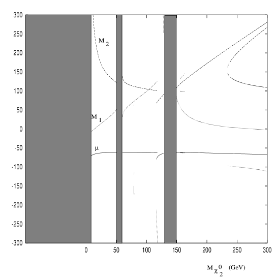
Figure 3: The parameters $\mu$, $M_{2}$ and $M_{1}$ as a function of $m_{\chi^{0}_{2}}$ for fixed $m_{\chi^{0}_{3}}=-100$ GeV and $m_{\chi^{\pm}_{1}}=80$ GeV for $\tan\beta=2$.

Finally, let us make a remark on the other MSSM parameters inversion. In parallel to the reconstruction of the gaugino sector soft–breaking parameters from the physical masses, it is natural to attempt such a reconstruction for the remaining part of the soft–breaking Lagrangian. In contrast to the gaugino sector however, the de–diagonalization of the sfermion sector and the Higgs sector does not present much analytical difficulties, provided of course that one knows a sufficient number of physical masses and/or couplings. Here, we briefly mention that such an inversion is indeed possible and we refer for more details and illustrations to Ref. [5]. We should only note that, in contrast with the gaugino sector inversion where the only difficulty was due to algebraically non–trivial de–diagonalization, for a realistic inversion of the Higgs parameters care should be taken with the correct account of one–loop corrections to the scalar potential and Higgs masses.

3.2 The program SUSPECT

3.2.1 Introduction

It is a well–known fact that the proliferation of Supersymmetry breaking terms in the unconstrained MSSM Lagrangian makes the Lagrangian–to–physical parameters [i.e. particles masses and couplings, etc.] relationship a rather tedious task to derive in an exhaustive manner. Although several systematic routines doing this work with different levels of refinement are available, it turned out to be highly desirable to develop our own tool within the GDR workshop, with the specific aim among other things, to fix a GDR–common set of parameter definitions and conventions once for all, and to have as much as possible flexibility on the input/output parameter choice.

Such a program should necessarily include the possibility of renormalization group evolution of the relevant parameters, due to the all importance of the high/low energy scales interplay in most modern SUSY scenarii, with GUT models as a typical but not only example. Besides, it unavoidably poses numerous questions on the relevance of various possible “options” [or more precisely model assumptions] to be available, as well as the choice of an adequate level of approximation at different stages, such as typically, in the effective potential related to radiative corrections to Higgs boson masses.

This brought us to develop the Fortran code SUSPECT which calculates the masses and couplings of the SUSY particles and the Higgs bosons of the MSSM. The code contains one source file [SUSPECT.f] and one input file [SUSPECT.in]; any choice and option is driven from this input file where one can change data almost at will. All results, including comments when useful, are to be found in the output file [SUSPECT.out] which is created at any run of the program. It is hoped that the code may be readily usable even with not much prior knowledge on the MSSM.

The code is as yet at a rather preliminary stage [version 1.1]. As mentioned previously, its main purpose at present is to propose some conventions, definitions, and possible flexibility choices which are largely open to discussions/suggestions. In the present version, only two extreme “models” are readily available: the “phenomenological MSSM” [but with the possibility of RG evolution to arbitrary scales] and the mSUGRA model; many “intermediate” models can be very easily included [suggestions are particularly welcome here]. For instance the pMSSM with unification of the gaugino masses at the GUT scale, or with a common scalar mass are straightforward to implement by just setting constraints “by hand” in the input file. The output for the MSSM mass spectrum has been compared with several other existing similar codes [see the “tools for SUSY” working group report [53] for more details on those comparisons], and is in reasonably good agreement. Up to a few percent differences in the output is to be sometimes expected, however, due to different approximations used in different codes.

The rest of this subsection is organized as follows: we first describe the most important subroutines in the case of the “phenomenological” MSSM in particular those which compute the chargino/neutralino, sfermion and Higgs boson masses and couplings. We will then discuss the case of the constrained MSSM with the various choices of approximations and refinements, paying a special attention on the RG evolution and the radiative electroweak symmetry breaking. Next, a description of the input and output files to be driven by the user is given. In doing so we shall try to be as close as possible to the definitions and conventions given in the previous subsections. We finally collect a list of various available [or not yet] options and/or model assumptions, with a clear mention of eventual limitations of the present version of the code.

3.2.2 The “phenomenological” MSSM

The purely phenomenological MSSM, that is, with the set of input parameters as defined in section 2.1, and without any RG evolution, is implemented by enforcing in the SUSPECT.in input file the choice ICHOICE(1)=0. Another alternative of interest is to have the full set of parameters as defined by the phenomenological model, but with the further possibility to evolve those parameters to –or from– an arbitrary scale prior to calculating the physical spectrum. This latter case is readily implemented and enforced by the choice ICHOICE(1)=1.

There are three main subroutines evaluating all possible SUSY physical masses, respectively chargino/neutralinos, Higgs boson and sfermion masses, for given input Lagrangian parameters:

       CALL GAUGINO(MU,M1,M2,M3,BETA,ALPHA,GMC,GMN,XMN)
       CALL SUSYCP(TGBETA)
       CALL SFERMION(MSQ,MTR,MBR,MSL,MTAUR,AL,AU,AD,MU,
     .               GMST,GMSB,GMSL,GMSU,GMSD,GMSE,GMSN)

For the couplings, only a subset is implemented at present: the couplings of the MSSM Higgs bosons to standard and SUSY particles [the angles $\alpha$ and $\beta\equiv{\rm atan}(\tan\beta)$ of the MSSM Higgs sector are called by a common]. Note that the couplings are not readily default output in the SUSPECT1.1 version, but are straightforwardly available, from various common blocks, as specified below. The remaining couplings [sfermion/ino couplings to gauge bosons and fermion–sfermion–ino] will be included soon.

In the subroutine GAUGINO, the input parameters are $\mu$, the gaugino masses $M_{1},M_{2},M_{3}$ [which can be made related], the mixing angles $\beta$ and $\alpha$ in the Higgs sector [the former is an input while the latter is calculated in the subroutine SUSYCP as explained below]. Signs and other relevant conventions are consistent with the ones discussed in section 3.1. The output is:

GMC(1), GMC(2): ordered values of the chargino masses
                  GMN(1)–GMN(4): ordered absolute values of the neutralino masses
                  XMN(1)–XMN(4): neutralino masses including the eventual negative signs.

The neutralino mass matrix is diagonalized analytically. The negative signs in XMN(1)–XMN(4) are relevant for instance for the couplings to Higgs bosons; if needed, these couplings are available via a common defined in the subroutine:

AC1(2,2),AC2(2,2),AC3(2,2): chargino–$h,H,A$ couplings
                  AN1(4,4),AN2(4,4),AN3(4,4): neutralino–$h,H,A$ couplings
                  ACNL(2,4),ACNR(2,4): chargino–neutralino–$H^{\pm}$ couplings.

The Higgs boson spectrum and couplings are calculated by the subroutine SUSYCP. It uses as two important input parameters: $\tan\beta$ and the mass of the pseudoscalar Higgs boson $M_{A}$ which may be either given as direct input or calculated from the two soft–SUSY breaking scalar masses $M_{H_{u}}$ and $M_{H_{d}}$ and $\mu$ as in eq. (2.31). In addition, SUSYCP uses as input the third generation soft scalar masses and trilinear couplings as well as $\mu$ which enter in the radiative corrections. In the case where the pole Higgs boson masses are calculated it needs the parameter $M_{2}$, as well as the masses of stops and sbottoms and their couplings to Higgs bosons [which are calculated similarly as in the subroutine SFERMION]. SUSYCP calls the subroutine SUBH [54], which calculates the renormalization group improved values of the Higgs boson masses and the couplings $\lambda$ in the scalar potential. The SUSYCP output gives the SM and $A,h,H,H^{\pm}$ Higgs boson masses and the running $A$ mass [the SM Higgs boson mass is in fact the input $M_{A}$]

AMSM,AMA,AML,AMH,AMHC,AMAR

Depending on the flag ICHOICE(10) one has either the running (=0) or pole (=1) Higgs boson masses masses [in the former case AMAR$\equiv$AMA]. The output also provides via common blocks the self–couplings $\lambda_{1-7}$ in the scalar potential, and the Higgs couplings to fermions, gauge bosons and the self–couplings [the notation being obvious, with T,B,L standing for $t,b,\tau$ and L,H,A for $h,H,A$; GLPM=$\sin(\beta-\alpha)$ and GHPM=$\cos(\beta-\alpha)$] as well as the running angles $\beta$ and $\alpha$:

COMMON/HMASS/AMSM,AMA,AML,AMH,AMCH,AMAR
COMMON/HSELF/LA1,LA2,LA3,LA4,LA5,LA6,LA7
COMMON/COUP/GAT,GAB,GLT,GLB,GHT,GHB,GZAH,GZAL,GHHH,GLLL,
                              GHLL,GLHH,GHAA,GLAA,GLVV,GHVV,GLPM,GHPM,B,A

In the subroutine SFERMION, the input parameters are the soft–SUSY breaking mass parameters for left–handed and right–handed squarks and sleptons, the trilinear couplings $A_{t},A_{b}$ and $A_{\tau}$ for the third generation and the parameter $\mu$. The output are 2–vectors:

GMST,GMSB,GMSL,GMSU,GMSD,GMSE,GMSN

for the masses of the two $\tilde{t},\tilde{b},\tilde{\tau}$ eigenstates, their first/second generation partners as well as the mass of the $\tilde{\nu}$’s. The D–terms are calculated by the subroutine and full mixing in the third generation is implemented. Again, the couplings to Higgs bosons are not explicitly written but are available if desired from a common defined in SFERMION:

GLEE(2,2),GLTT(2,2),GLBB(2,2): $h$ couplings to $\tilde{\tau},\tilde{t},\tilde{b}$
                  GHEE(2,2),GHTT(2,2),GHBB(2,2): $H$ couplings to $\tilde{\tau},\tilde{t},\tilde{b}$
                  GAEE,GATT,GABB: $A$ couplings to $\tilde{\tau}_{1}\tilde{\tau}_{2}$, $\tilde{t}_{1}\tilde{t}_{2}$, $\tilde{b}_{1}\tilde{b}_{2}$
                  GCEN(2,2),GCTB(2,2): $H^{\pm}$ couplings to $\tilde{\tau}\tilde{\nu}$, $\tilde{t}\tilde{b}$.

The conventions for the signs of $A_{f},\mu$ as well as the mixing terms are as introduced previously. [The sfermion masses are running masses, since they are obtained from the Lagrangian parameters of the scalar sector; note indeed that for stops and sbottoms the running quark partner masses are implemented in the mass matrices].

Of course, the three subroutines need in addition some standard input parameters. Apart from “electroweak” coupling constant inputs [such as the Fermi constant or the QED coupling defined at zero–momentum] and some particles masses [such as the W,Z gauge boson and fermion masses] which are precisely known and which are included in the source code, there are other less precisely known parameters which are very important [especially in the constrained MSSM, since e.g. the GUT and SUSY thresholds are quite sensitive to the values of some of them]. These constants [defined at the low scale, where they are experimentally measured, currently $M_{Z}$] are:

ALFINV: the inverse QED constant $1/\alpha(M_{Z})$ in the $\overline{\rm MS}$ scheme (=127.9)
          SW2: $\sin^{2}\theta_{W}(M_{Z})$ in the $\overline{\rm MS}$ scheme (=0.2315 for $m_{t}=175$ GeV);
          ALPHAS: the value of $\alpha_{S}(M_{Z})$ at the $M_{Z}$ scale (=0.119 );
          MT,MB,MC: the $t,b,c$ pole masses (=175, 4.7, 1.42 GeV)

The reference values for those parameters as indicated in parenthesis above correspond to central values quoted by the most recent data [55]; they may accordingly be varied within the known error bounds.

3.2.3 Constrained MSSM

The case of mSUGRA is dealt with by the flag ICHOICE(1)=10 in SUSPECT.in. In the mSUGRA choice, all the SUSY parameters are determined in terms of four arbitrary and one discrete parameters which are given at a “high” scale which, if unification of the gauge couplings is imposed, corresponds to the GUT scale $M_{U}$. These parameters, as discussed in section 2.1, are:

                 TGBETA(MZ), m0(GUT), mHALF(GUT), A0(GUT), sign(MU)

Other parameters also enter the game as “starting guess” values, and must be specified in some cases:

                      MU, B, SUSYM, EHIGH, ELOW

Typically, the actual values of $\mu$ and $B$ are determined consistently from EWSB, but the latter almost unavoidably needs some iteration procedure, and thus some starting “seed” $\mu,B$ values are necessary. If the unification of the gauge couplings scenario is not chosen two additional inputs must be given: SUSYM corresponding to an initial guess of the SUSY threshold [a single universal one to simplify], and EHIGH corresponding to the high energy end of the RG evolution [if gauge unification is enforced, both SUSYM and EHIGH can be safely set to arbitrary values, as more adequate values will be then calculated]. Finally, one needs to specify ELOW which corresponds to the lower–energy end of the RG evolution equations; this is always necessary and important as it fixes the final scale at which all physical masses will be computed. Moreover, ELOW should be below or at most equal to the EWSB scale [see the discussion in section 2.2]. Thus ELOW should be roughly of the order of the electroweak scale, with some flexibility, say $M_{Z}<{\rm ELOW}<1000$ GeV. In the mSUGRA case all other parameters are then determined by GUT universality and RG evolution.

In addition, independently of the model choice driven by ICHOICE(1), there are several possibilities for the RG evolution equations and for electroweak symmetry breaking [which are however not always all relevant, depending on the choice of models]:

• ICHOICE(2): elaboration level of the RG evolution equations.
  =11 (21): one (two)–loop evolution with simple [single SUSY–threshold scale] threshold effects.
  =12 (22): one (two)–loop evolution, with more realistic thresholds [i.e. step functions for each particle specy thresholds].

• ICHOICE(3): Gauge coupling and Yukawa coupling unification.
  = 0: no unification
  = 1: only gauge coupling unification [then approximate GUT and simple SUSY–threshold scales are automatically determined].
  = 2: gauge and bottom–tau Yukawa coupling unification

• ICHOICE(4): Accuracy of RG evolution.
  = 0: fast but less accurate RG evolution.
  = 1: accurate evolution but rather slow.

• ICHOICE(5): for electroweak symmetry breaking.
  =0: no radiative EWSB [electroweak breaking is of course there and determines consistent values of $B$ and $\mu$ at the EWSB scale; the difference between “radiative” and “no radiative” EWSB was explained in section 2.2].
  =1: radiative EWSB is implemented, i.e. $B$ and $\mu$ are fixed at the EW scale and by other parameters to be consistent with RG evolution from a given (generally EHIGH $\simeq M_{U}$) scale. [NB: ICHOICE(5)=1 is automatically enforced for the mSUGRA case ICHOICE(1)=10]

• ICHOICE(6)–ICHOICE(9) are reserved for later use.

• ICHOICE(10): =0 (1) computes running (pole) Higgs boson masses.

Note that we anticipated several possible steps between the pMSSM and mSUGRA and therefore left the possibilities ICHOICE(6–9) reserved for later use. Besides the physical spectrum calculation for input Lagrangian parameters as described above, the two other main tasks performed by the code are the RG evolution of the parameters, and the consistent implementation of EWSB, which we discuss is some more details now.

(i) Renormalization Group evolution:

ODEINT is a subroutine returning a set of masses and coupling parameters at a specified scale $Q_{\rm out}$, when given at an initial scale $Q_{\rm in}$. It is based on a Runge–Kutta numerical algorithm solving differential equations by Numerical Recipes [56]. RG evolution is trivially reversible, so that the choice of $Q_{\rm in}$ and $Q_{\rm out}$ is in principle quite flexible; it is also possible in particular to use this evolution back and forth if needed.

       CALL ODEINT(y,n,x1,x2,eps,h1,1.d-5,nok,nbad,deriv1,rkqc)

The input are the values $y(n)$ of all evolving couplings and masses relevant to the phenomenological MSSM, given at the scale $Q_{in}=e^{x_{1}}$, the latter being also given as input; see section 2.3 for the precise assignment of $y(n)$ components in terms of MSSM couplings and masses. [Quite obviously, when specific constraints on the $y(n)$ are implemented at some scale, like in the mSUGRA model typically, it simply implies specific initial conditions for those. But the evolution of each mass or coupling parameters is driven by its own specific beta function and we therefore should keep the latter as model–independent as possible]. The output are the values of $y(n)$ at the scale $Q_{\rm out}=e^{x_{2}}$ to be specified.

According to the previous discussion ODEINT also needs the beta functions: $\beta(y)(\equiv d(y)/d\ln Q$), for all the relevant $y(n)$, which are provided by the subroutines:

                    subroutine DERIV1(x,y,dydx)
                    subroutine DERIV2(x,y,dydx)

for the one and two-loop RG beta functions respectively, including threshold effects.

(ii) Electroweak Symmetry Breaking:

There is a set of subroutines [in fact essentially one] which evaluates the one–loop contribution to the effective potential, whose detailed shape study settles the occurrence [or not] of the ${\rm SU(2)\times U(1)}$ spontaneous symmetry breaking, irrespective of particular model building assumptions. What is however, a model assumption chosen as option flag, is whether the EWSB is radiative or not; namely whether the relevant parameters of the Higgs potential at the EWSB scale are consistent or not with their respective values chosen at a higher scale, given their specific RG evolution properties [see again section 2.2 for a more complete discussion on EWSB].

       call VLOOP2(Q2,mt2,mst22,mst12,mb2,msb22,msb12,
     .        mtau2,mstau22,mstau12,-rmu,dVdvd2,dVdvu2)

The inputs are:

Q2: the scale $Q^{2}$ ($\geq$ ELOW) at which EWSB is supposed to happen;
                  mt2, mst22, mst12: the $t,\tilde{t}_{1},\tilde{t}_{2}$ masses;
                  mb2, msb22, msb12: the $b,\tilde{b}_{1},\tilde{b}_{2}$ masses;
                  mtau2, mstau22, mstau12: the $\tau,\tilde{\tau}_{1},\tilde{\tau}_{2}$
                  $-$RMU: the parameter $\mu$

The output are dVdvd2, dVdvu2, which are [up to some appropriate overall constants] the derivatives $\partial(V_{\rm eff})/\partial(v^{2}_{d})$, $\partial(V_{\rm eff})/\partial(v^{2}_{u})$ respectively, the basic quantities entering Higgs mass corrections and EWSB consistency conditions. As already mentioned, our present algorithm calculates values of the parameters $B$ and $\mu$ consistent with EWSB by iterating the two expressions of $\mu^{2}$ and $B$, eqs. (2.31) of section 2.2. The iteration is non trivial because in eqs. (2.31):

$$\tilde{M}^{2}_{H_{d}}\equiv M^{2}_{H_{d}}+\partial(V_{\rm eff})/\partial(v^{2}_{d})\ \ {\rm and}\ \ \tilde{M}^{2}_{H_{u}}\equiv M^{2}_{H_{u}}+\partial(V_{\rm eff})/\partial(v^{2}_{u})$$ (3.59)

involve other MSSM particle masses and couplings, which themselves depend on $\mu$ [in most practical cases, however, the algorithm converges very fast, after 2 or 3 iterations]. Besides eqs. (2.31), there are other constraints to fulfill in order to assert that one reached a local minimum of the potential, as discussed in section 2.2. This is simply checked numerically in SUSPECT. In contrast, there is no consistency checks about the possible occurrence of charge and color breaking [CCB] minima in the present version 1.1. Note, however, that a more refined different algorithm, partly based on analytical studies of the complete potential at its minimum [2], will be implemented later.

3.2.4 Example of input/output files

The following example of SUSPECT.in input file, corresponds to the mSUGRA so–called “SNOWMASS” point 1:

1) choice of different options/models, etc flags:
ICHOICE(1) = 10
ICHOICE(2) = 21
ICHOICE(3) = 12
ICHOICE(4) = 0
ICHOICE(5) = 1
ICHOICE(6) = 0
ICHOICE(7) = 0
ICHOICE(8) = 0
ICHOICE(9) = 0
ICHOICE(10)= 1

2) Initialize SM parameters:
ALFINV   =127.9d0
SW2      =.2315d0
ALPHAS   =.12d0
MT       =175.d0
MB       = 4.7d0
MC       =1.42d0

3) Initialize SUSY parameters
SUSYM    = 200.d0
EHIGH(GUT=2.d16
ELOW     = 433.d0
(here SUGRA case with universality):
m0       = 400.d0
m1/2     = 200.d0
A0       = 0.d0
TGBETA   = 2.d0
SGNMU0   = -1.d0

4) pMSSM case (at HIGH scale!)
MHU2     = .5D4
MHD2     = 5.d5
M1       = 200.D0
M2       = 200.D0
M3       = 200.D0
MSL      = 1.D2
MTAUR    = 1.D2
MSQ      = 1.d2
MTR      = 1.d2
MBR      = 1.D2
MEL      = 1.D2
MER      = 1.D2
MUQ      = 1.D2
MUR      = 1.D2
MDR      = 1.D2
AL       = 200.D0
AU       = 200.D0
AD       = 200.D0

The corresponding SUSPECT.out output file is shown below [the comments are self–explanatory]:

 HIGH(GUT), LOW (Final) and SUSY-threshold     SCALES:
  0.274650E+17    433.000        175.000
 EVOLVE FIRST TIME from MZ to HIGH(GUT) scale
 gauge cpl^2 1,2,3 at HIGH(GUT) scale  0.529596 0.526736 0.517345
 RUNNING mtau,mb,mtop at HIGH scale    1.58621  1.18050  76.0442
 EVOLVE DOWN to Low-energy

__________________________________________________________________
            RESULTING values at Low-energy scale:
 tan(beta) at Low scale:    1.93532
 mtau,mb,mtop at Low scale:    1.76582        2.69798        151.422
 Atau,Ab,Atop at Low scale:   -135.228       -633.479       -368.151
 m(phi_u)^2, m(phi_d)^2   -137416.        179919.
 m_tauR, m_L, m_bR, m_tR, m_Q:
   407.225      424.685      607.580      399.425      530.837
 rel. % err. in B, mu:   0.280874E-03    0.338679E-03
 (indicate departure from consistent radiative  EW breaking)
 loop-level EW breaking + stability tests:
 m1^2*m2^2-B^2*MU^2, m1^2+m2^2 +/-2*B*MU:
 -0.767807E+09   994235.       100948.
 FINAL SOFT-BREAKING PARAMETERS:
 mu(Q_EWB), B(Q_EWB):   -504.916       -442.295
 gauginos 1,2,3 masses:    83.3875        165.443        524.285

 __________________________________________________________________
            FINAL PHYSICAL PARAMETER RESULTS:
    tgbeta       M_A        M_h       M_H        M_H+
      2.000   735.902    79.555   742.020   743.895

    chi_+^1    chi_+^2    chi_0^1    chi_0^2    chi_0^3    chi_0^4
   172.336   515.130    85.597   172.466   506.938   516.171

   stop_1     stop_2     sup_1      sup_2
   429.182   557.382   621.448   608.878

   sbottom_1  sbottom_2    sdown_1    sdown_2
   532.761   607.879   624.448   608.114

    stau_1     stau_2    selec_1    selec_2      sneut
   408.361   426.429   426.354   408.756   421.948
 __________________________________________________________________

3.2.5 Discussions and outlook

In summary, the main core of the code SUSPECT gives the physical masses and couplings of the SUSY particles and the MSSM Higgs bosons as functions of input Lagrangian parameters, taking into account renormalization group evolution if needed, and consistent electroweak symmetry breaking. In addition, there are a number of options, which might be useful for many practical purposes, that we briefly describe now.

INVERTOR:

This is a subroutine [based on the discussion in section 3.1.2], which will be included soon in the next version, as an option in SUSPECT and whose purpose is to determine the inverted spectrum relationship [i.e. recovering the Lagrangian parameter values directly from physical masses and/or couplings]. The algorithm in its present form essentially deals with the non–trivial inversion in the gaugino parameter sector, where the input can be either two charginos and one neutralino, or two neutralinos and one chargino physical masses. The output are the Lagrangian gaugino parameters, $\mu$, $M_{1}$, $M_{2}$ [the $M_{3}$ to $M_{\rm gluino}$ relation obviously does not need inversion].

RGEXACT:

This is a subroutine also to be included in the next version as an option in SUSPECT which implements an exact RG evolution solver [limited to one–loop approximation]. We refer to section 2.3 for a more detailed discussion of the procedure. Let us simply mention here, that the exact solutions of the relevant SUSY RG equations which have been recently derived for arbitrary values of $\tan\beta$, should not only be useful to improve the general RG evolution algorithm, but more importantly, should provide a better control on some non–trivial issues of the RG evolution, such as the possible occurrence of Landau poles in the Yukawa couplings typically.

Finally we emphasize that the code is largely in a developing stage, and many other extensions of the present algorithms and options are foreseen, as well as interfaces with other numerical codes for SUSY. Some of the present limitations and approximations of the version SUSPECT1.1 are:

(i) Model choice:

Only two extreme “models”, phenomenological MSSM on one side and mSUGRA with all universal terms on the other side, are treated at present. Many “intermediate” models can be enforced by hand by choosing appropriately the input parameters and will be very easily included later.

(ii) Scale choice:

The input scale at which to define parameters is not at present completely flexible: in the phenomenological MSSM, all SUSY parameters should be entered at the same scale [the latter scale is however arbitrary, provided it is chosen between 1 TeV and say $10^{18}$ GeV]. An important exception is $\tan\beta$, which should be given at the $Z$–boson scale and of course the SM parameters such as $\alpha_{s}$, etc.. [see the example of input file].

(iii) Approximations in specific calculations:

There are approximations in the RG evolution, for instance an option on one–loop versus two–loop evolution, where in the latter only the gauge and Yukawa couplings truly involve two–loop contributions. Also, there are approximations in the contributions to the one–loop corrections to the scalar potential [relevant for the radiative EWSB consistency conditions]: that is, only the third generation fermion and sfermion contributions are included. This implies, strictly speaking, some inconsistency with the RG evolution since in the latter much more contributions are taken into account. The inconsistency however, should not be very significant numerically. A more complete and consistent treatment of the one–loop scalar effective potential will be available in the next version of the program.

(iv) Threshold effects:

These are not yet fully realistic at the present moment: only a single, average SUSY threshold scale can be chosen. Inclusion of more realistic thresholds [i.e. for each particle species] will be soon available.

(v) Electroweak symmetry breaking:

As explained previously, the EWSB conditions are consistently implemented numerically by iteration on the parameters $\mu$ and $B$, and the occurrence of a local minimum is checked numerically. There is however, no check about the possible occurrence of inconsistent charge and color breaking minima in the present version. These should be implemented in the next version, together with a complete and more analytical treatment of the EWSB conditions.

(vi) Known bugs:

Finally to be fair one cannot omit mentioning that one serious bug that has been identified in this 1.1 version, is not yet completely understood. The observation is that, for some choices of the low scale input parameters, and in particular for a relatively low value of $\tan\beta$, $\raisebox{-3.69899pt}{~{}\shortstack{$<$ \\ [-0.07cm] $\sim$}}~{}1.3$–$1.4$, there is an uncontrollable growth of the Yukawa/gauge couplings, when running the RGE in the upwards direction. This seemingly “Landau pole” effects is not yet under control and we hope to solve this problem for the next version [the exact RG solver RGEXACT will certainly help us to resolve the issue].

The next version SUSPECT1.2 should therefore be hopefully more complete.

4. Higgs Boson Production and Decay

One of the main motivations of supersymmetric theories, as discussed in section 2, is the fact that they provide an elegant way to break the electroweak symmetry and to stabilize the huge hierarchy between the GUT and Fermi scales [21, 22]. The probing of the Higgs sector of the MSSM [23] is thus of utmost importance. The search for the CP–even Higgs bosons $h$ and $H$, the pseudoscalar Higgs boson $A$ and the charged Higgs particles $H^{\pm}$ of the MSSM is therefore one of the main entries in the LEP2 [57], Tevatron [58], LHC [59, 60] and future $e^{+}e^{-}$ colliders [61] agendas.

In the theoretically well motivated models, such as the mSUGRA scenario discussed previously, the MSSM Higgs sector is in the so called decoupling regime [62] for most of the SUSY parameter space allowed by present data constraints [55]: the heavy CP–even, the CP–odd and the charged Higgs bosons are rather heavy and almost degenerate in mass, while the lightest neutral CP–even Higgs particle reaches its maximal allowed mass value $M_{h}\raisebox{-3.69899pt}{~{}\shortstack{$<$ \\ [-0.07cm] $\sim$}}~{}$ 80–130 GeV [48, 49] depending on the SUSY parameters. In this scenario, the $h$ boson has almost the same properties as the SM Higgs boson and would be the sole Higgs particle accessible at the next generation of colliders.

In this section, we discuss the production of the MSSM Higgs bosons at the next generation of colliders, mainly at the LHC and a future $e^{+}e^{-}$ linear collider as well as their decays modes, in particular the SUSY channels. The new material presented in this section is based on Refs. [7, 8, 9, 10, 11].

4.1 MSSM Higgs boson production at the LHC

4.1.1 Physical set–up

At the LHC, the most promising channel [59, 60] for detecting the lightest $h$ boson is the rare decay into two photons, $h\rightarrow\gamma\gamma$, with the Higgs particle dominantly produced via the top quark loop mediated gluon–gluon fusion mechanism [63, 64]

$$gg\rightarrow h$$ (4.1)

In the decoupling regime, the two LHC collaborations expect to detect the narrow $\gamma\gamma$ peak in the entire Higgs mass range, 80 $\raisebox{-3.69899pt}{~{}\shortstack{$<$ \\ [-0.07cm] $\sim$}}~{}M_{h}\raisebox{-3.69899pt}{~{}\shortstack{$<$ \\ [-0.07cm] $\sim$}}~{}130$ GeV, with an integrated luminosity $\int{\cal L}\sim 300$ fb^-1 corresponding to three years of LHC running [59]; see Fig. 4.

Two other channels can be used to detect the $h$ particle in this mass range: the production in association with a $W$ boson [65] or in association with top quark pairs [66]

$$pp\ \rightarrow\ hW\ \ \ {\rm and}\ \ \ pp\rightarrow\bar{t}th$$ (4.2)

with the $h$ boson decaying into 2 photons and the $t$ quarks into $b$ quarks and $W$ bosons [for the latter process, the Higgs boson detection with $h\rightarrow b\bar{b}$ final states looks also promising; see Ref. [67] for instance]. Although the cross sections are smaller compared to the $gg\rightarrow h$ case, the background cross sections are also small if one requires a lepton from the decaying $W$ bosons as an additional tag, leading to a significant signal. Furthermore, the cross section $\sigma(pp\rightarrow\bar{t}th)$ is directly proportional to the top–Higgs Yukawa coupling, the largest electroweak coupling in the SM; this process would therefore allow the measurement of this parameter, and the experimental test of a fundamental prediction of the Higgs mechanism: the Higgs couplings to fermions and gauge bosons are proportional to the particle masses.

The additional vector boson fusion mechanisms [68],

$$pp\rightarrow W^{*}W^{*}/Z^{*}Z^{*}\rightarrow qqh$$ (4.3)

is less interesting to detect the $h$ boson than in the SM, but can be useful to test the $h$ particle properties [for instance to measure the $hWW$ and $hZZ$ couplings].

The heavy CP–even $H$ and CP–odd $A$ bosons can be searched for at the LHC through their decays modes into $\tau^{+}\tau^{-}$ pairs with the Higgs bosons produced in the $gg$ fusion mechanism or in association with $b\bar{b}$ pairs:

$$gg\rightarrow H/A\ \ \ {\rm and}\ \ \ gg,q\bar{q}\rightarrow b\bar{b}\;+\;H/A$$ (4.4)

This needs large values $\mbox{tan}\beta\raisebox{-3.69899pt}{~{}\shortstack{$>$ \\ [-0.07cm] $\sim$}}~{}5$ for the Higgs boson masses $M_{H,A}\raisebox{-3.69899pt}{~{}\shortstack{$>$ \\ [-0.07cm] $\sim$}}~{}300$ GeV, to enhance the cross sections of the above processes and the $\tau^{+}\tau^{-}$ decay branching ratios, which in the case where only standard modes are allowed reach the asymptotic value of $\sim 10\%$ [69]. The decays of the $H$ and $A$ bosons into muon pairs, $H/A\rightarrow\mu^{+}\mu^{-}$, give a rather clean signal and can be used despite of the very small branching ratios, $\sim 4.10^{-4}$ in the asymptotic limit. For lower values $\mbox{tan}\beta\raisebox{-3.69899pt}{~{}\shortstack{$<$ \\ [-0.07cm] $\sim$}}~{}3$ [most of which will be covered by the upgrade of LEP to $\sqrt{s}=200$ GeV] and not too large $M_{H,A}$ values, the decays $H/A\rightarrow t\bar{t}$ can be also used. The decays $H\rightarrow hh\rightarrow b\bar{b}\gamma\gamma$ and $A\rightarrow Zh\rightarrow l^{+}l^{-}b\bar{b}$ can also be used in a tiny area of the MSSM parameter space; see Fig. 4.

At the LHC, the only way to detect the charged Higgs boson is when $M_{H^{\pm}}<m_{t}-m_{b}$ and the $H^{\pm}$ particles can be then produced in top quark decays,

$$pp\ \rightarrow\ t\bar{t}\ \ {\rm with}\ \ t\rightarrow H^{+}b$$ (4.5)

The usual signature is to look at a breakdown of lepton universality by selecting the decay $H^{+}\rightarrow\tau^{+}\nu_{\tau}$, which together with the decay $H^{+}\rightarrow c\bar{s}$ for small $\mbox{tan}\beta$ values, is considered as the main decay mode [see however the discussion in section 4.2]; Fig. 4.

In the next subsections we will discuss the effects of supersymmetric particles in the production of the lightest $h$ boson at the LHC: first the contributions of light stops in the production of the $h$ boson in the $gg\rightarrow h$ mechanism which can significantly alter the expected production rate [7] and then the associated production of the $h$ boson with $\tilde{t}$–squark pairs for which the cross section can be rather large, exceeding the one for the SM–like process $pp\rightarrow t\bar{t}h$ [8].

One of the most important ingredients of these discussions is that stops can alter significantly the phenomenology of the MSSM Higgs bosons. The reason is two–fold: $(i)$ as discussed in section 3.1, the current eigenstates, $\tilde{t}_{L}$ and $\tilde{t}_{R}$, mix to give the mass eigenstates $\tilde{t}_{1}$ and $\tilde{t}_{2}$; the mixing angle $\theta_{\tilde{t}}$ is proportional to $m_{t}\tilde{A}_{t}$, with $\tilde{A}=A_{t}-\mu/\tan\beta$, and can be very large, leading to a scalar top squark $\tilde{t}_{1}$ much lighter than the $t$–quark and all other scalar quarks; $(ii)$ the couplings of the top squarks to the neutral Higgs bosons $h$ given in section 3.1, involve components which are proportional to $\tilde{A}_{t}$ and for large values of this parameter, the $g_{h\tilde{t}_{1}\tilde{t}_{1}}$ coupling can be strongly enhanced.

The strong $h$ couplings to stops would result in a stop contribution to the $hgg$ and $h\gamma\gamma$ vertices that is comparable or even larger than the top contribution, altering significantly the rate for the process $gg\rightarrow h\rightarrow\gamma\gamma$. It also leads to a possibly substantial cross section for the production of the $h$ boson in association with stops, $pp\rightarrow\tilde{t}\tilde{t}h$.

Figure 4: MSSM parameter space with the contours of the Higgs bosons visible at the LHC with a luminosity $\int{\cal L}dt=300$ fb^-1 and combining the experimental data of ATLAS and CMS; from Ref. [70].

4.1.2 Higgs production in the gluon fusion mechanism

In the SM, the Higgs–gluon–gluon vertex is mediated by heavy [mainly top and to a lesser extent bottom] quark loops, while the rare decay into two photons is mediated by $W$–boson and heavy fermion loops, with the $W$–boson contribution being largely dominating. In the MSSM however, additional contributions are provided by SUSY particles: $\tilde{q}$ loops in the case of the $hgg$ vertex, and $H^{\pm},\tilde{f}$ and $\chi^{\pm}$ loops in the case of the $h\rightarrow\gamma\gamma$ decay. In the latter case [71], the contributions of $H^{\pm}$ bosons, sleptons and the scalar partners of the light quarks are in general small given the experimental bounds on the masses of these particles [55]. Only the contributions of relatively light $\tilde{t}$ squarks [and to a lesser extent $\tilde{b}$ for large $\tan\beta$ values and $\chi_{1}^{\pm}$ for masses close to 100 GeV, which could contribute at the 10% level] can alter significantly the loop induced $hgg$ and $h\gamma\gamma$ vertices.

The expressions of the partial width for the decay $h\rightarrow gg$, can be found in Ref. [64]; the cross section $\sigma(gg\rightarrow h$) is directly proportional to the decay width $\Gamma(h\rightarrow gg)$. The latter cross section is affected by large QCD radiative corrections [64]; however they are practically the same for quark and squark loops, and if only deviations compared to the standard case are considered, they drop out in the ratios. The partial width for the decay $h\rightarrow\gamma\gamma$ can be found e.g. in Ref. [71]; the QCD corrections are small and can be neglected. The $\gamma\gamma$ and $gg$ decay widths of the $h$ boson are evaluated numerically with the help of an adapted version of the program HDECAY [72].

Figs. 5 and 6 show, as a function of $\tilde{A}_{t}$ for $\mbox{tan}\beta=2.5$, the deviations from their SM values of the partial decay widths of the $h$ boson into two photons and two gluons as well as their product which gives the cross section times branching ratio $\sigma(gg\rightarrow h\rightarrow\gamma\gamma)$. The quantities $R$ are defined as the partial widths including the SUSY loop contributions [all charged SUSY particles for $h\rightarrow\gamma\gamma$ and squark loops for $h\rightarrow gg$] normalized to the partial decay widths without the SUSY contributions, which in the decoupling limit correspond to the SM contributions: $R=\Gamma_{\rm MSSM}/\Gamma_{\rm SM}$.

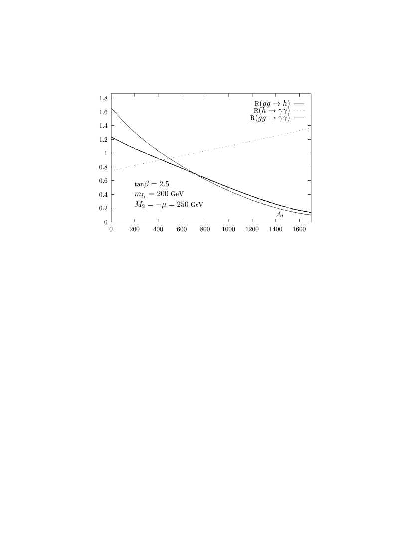
Figure 5: SUSY loop effects on R$(gg\rightarrow h)$, R$(h\rightarrow\gamma\gamma)$ and R$(gg\rightarrow\gamma\gamma)$ as a function of $\tilde{A}_{t}$ for $\mbox{tan}\beta=2.5$ and $m_{\tilde{t}_{1}}=200$ GeV, $M_{2}=-\mu=250$ GeV.

Figure 6: SUSY loop effects on R$(gg\rightarrow\gamma\gamma)$ as a function of $\tilde{A}_{t}$ for $\mbox{tan}\beta=2.5$ and $m_{\tilde{t}_{1}}=165,400$ and 600 GeV with $M_{2}=-\mu=500$ GeV for $m_{\tilde{t}_{1}}\geq 400$ GeV.

In Fig. 5, the stop mass is set to $m_{\tilde{t}_{1}}=200$ GeV. For small values of $\tilde{A}_{t}$ there is no mixing in the stop sector and the dominant component of the $h\tilde{t}\tilde{t}$ couplings, eq. (3.48), is the one proportional to $m_{t}^{2}/M_{Z}^{2}$ [here, both $\tilde{t}_{1}$ and $\tilde{t}_{2}$ contribute since their masses and couplings to $h$ are almost the same]. The sign of this component, compared to the $ht\bar{t}$ coupling, is such that the $t$ and $\tilde{t}$ contributions interfere constructively in the $hgg$ and $h\gamma\gamma$ amplitudes. This leads to an enhancement of the $h\rightarrow gg$ decay width up to $60\%$ in the MSSM. However, the $h\rightarrow\gamma\gamma$ decay width is dominated by the $W$ amplitude which interferes destructively with the $t$ and $\tilde{t}$ amplitudes, and the $\tilde{t}$ contributions reduce the $h\rightarrow\gamma\gamma$ decay width by an amount up to $-20\%$. The product R($gg\rightarrow\gamma\gamma$) in the MSSM is then enhanced by a factor $\sim 1.2$ in this case.

With increasing $\tilde{A}_{t}$, the two components of $g_{h\tilde{t}_{1}\tilde{t}_{1}}$ [which have opposite sign since $\sin 2\theta_{\tilde{t}}\propto m_{t}\tilde{A}_{t}$ in eq. (3.48)] interfere destructively and partly cancel each other, resulting in a rather small stop contribution. For larger values of $\tilde{A}_{t}$, the second component of $g_{h\tilde{t}_{1}\tilde{t}_{1}}$ becomes the most important one, and the $\tilde{t}_{1}$ loop contribution [$\tilde{t}_{2}$ is too heavy to contribute] interferes destructively with the one of the $t$–quark. This leads to an enhancement of R$(h\rightarrow\gamma\gamma)$ and a reduction of R$(gg\rightarrow h)$. However, the reduction of the latter is much stronger than the enhancement of the former [recall that the $W$ contribution in the $h\rightarrow\gamma\gamma$ decay is much larger than the $t$ contribution] and the product R($gg\rightarrow\gamma\gamma$) decreases with increasing $\tilde{A}_{t}$. For $\tilde{A}_{t}$ values of about 1.5 TeV, the signal for $gg\rightarrow h\rightarrow\gamma\gamma$ in the MSSM is smaller by a factor of $\sim 5$ compared to the SM case.

Fig. 6 shows the deviation R$(gg\rightarrow\gamma\gamma)$ with the same parameters as in Fig. 5 but with different $\tilde{t}_{1}$ masses, $m_{\tilde{t}_{1}}=165,400$ and 600 GeV. For larger masses, the top squark contribution $\propto 1/m_{\tilde{t}_{1}}^{2}$, will be smaller than in the previous case. In the no–mixing case, the enhancement (reduction) of the $hgg(h\gamma\gamma)$ amplitude is only of the order of 10% for $m_{\tilde{t}_{1}}\simeq 400$ GeV, and leads to an almost constant cross section times branching ratio for the $gg\rightarrow h\rightarrow\gamma\gamma$ process compared to the SM case. Again the stop contribution vanishes for some intermediate value of $\tilde{A}_{t}$, and then increases again in absolute value for larger $\tilde{A}_{t}$. However, for $m_{\tilde{t}_{1}}\simeq 400$ GeV, the effect is less striking compared to the case of $m_{\tilde{t}_{1}}=200$ GeV, since here $\sigma(gg\rightarrow h)\times{\rm BR}(h\rightarrow\gamma\gamma$) drops by less than a factor of 2, even for extreme values of $\tilde{A}_{t}\sim 2.5$ TeV. As expected, the effect of the top squark loops will become less important if the $\tilde{t}_{1}$ mass is increased further to 600 GeV for instance. In contrast, if the stop mass is reduced to $m_{\tilde{t}_{1}}\simeq 165$ GeV, the drop in R$(gg\rightarrow\gamma\gamma)$ will be even more important: for $\tilde{A}_{t}\sim 1.5$ TeV, the $gg\rightarrow\gamma\gamma$ cross section times branching ratio including stop loops is an order of magnitude smaller than in the SM. For $\tilde{A}_{t}\sim 1.3$ TeV, the $\tilde{t}$ amplitude almost cancels completely the $t/b$ quark amplitudes; the non–zero value of R$(gg\rightarrow\gamma\gamma)$ is then due to the imaginary part of the $b$-quark contribution.

One should recall that $M_{h}$ varies with $\tilde{A}_{t}$, and no constraint on $M_{h}$ has been set in Figs. 5–6. Requiring $M_{h}\raisebox{-3.69899pt}{~{}\shortstack{$>$ \\ [-0.07cm] $\sim$}}~{}90$ GeV, the lower range $\tilde{A}_{t}\raisebox{-3.69899pt}{~{}\shortstack{$<$ \\ [-0.07cm] $\sim$}}~{}350$ GeV and the upper ranges $\tilde{A}_{t}\raisebox{-3.69899pt}{~{}\shortstack{$>$ \\ [-0.07cm] $\sim$}}~{}1.5(2.3)$ TeV for $m_{\tilde{t}_{1}}=200(400)$ GeV for instance, are ruled out. This means that the scenario where R$(gg\rightarrow\gamma\gamma)>1$, which occurs only for $\tilde{A}_{t}\raisebox{-3.69899pt}{~{}\shortstack{$<$ \\ [-0.07cm] $\sim$}}~{}300$ GeV for $m_{\tilde{t}_{1}}=200$ GeV is ruled out for $M_{h}\raisebox{-3.69899pt}{~{}\shortstack{$>$ \\ [-0.07cm] $\sim$}}~{}90$ GeV. Therefore, the rate for the $gg\rightarrow\gamma\gamma$ process in the MSSM will always be smaller than in the SM case, making more delicate the search for the $h$ boson at the LHC with this process.

For large values of $\mbox{tan}\beta$, $\mbox{tan}\beta\gg 1$, the mixing in the sbottom sector can also be very large, leading to $m_{\tilde{b}_{1}}$ possibly rather small, and a large $g_{h\tilde{b}_{1}\tilde{b}_{1}}$ coupling which can also generate large $\tilde{b}_{1}$ loop contributions to the $hgg$ and $h\gamma\gamma$ vertices. Indeed, for $\mbox{tan}\beta\sim 50$ and $m_{\tilde{b}_{1}}=200$ GeV, the deviations of the R$(h\rightarrow gg)$ and thus R$(gg\rightarrow h\rightarrow\gamma\gamma$) observables from unity are substantial for large values of $|\mu|$. For instance, for $|\mu|\simeq 1$ TeV the $gg\rightarrow\gamma\gamma$ cross section in the MSSM can be suppressed compared to the SM case by a factor of 5. When $m_{\tilde{b}_{1}}$ is increased (reduced) the effect becomes less (more) striking.

In the case where the decoupling limit is not yet reached, the $hWW$ and $htt$ couplings are smaller than in the SM, and both the $gg\rightarrow h$ cross section and $h\rightarrow\gamma\gamma$ widths are suppressed compared to the SM case, even in the absence of the squark loops. Including light $\tilde{t}$ contributions will further decrease the amplitudes for large $\tilde{A}_{t}$. For large $\mbox{tan}\beta$ values, the $hgg$ amplitude can be enhanced by the $b$–loop contribution, but the $h\rightarrow\gamma\gamma$ branching ratio is strongly suppressed due to the absence of the $W$–loop and the increase of the total decay width $\propto m_{b}^{2}\tan^{2}\beta$.

Finally, in the case of the heavy $H$ boson, squark loop contributions to the cross section $gg\rightarrow H$ can be even larger since because of the larger value of $M_{H}$, more room will be left for the $\tilde{t}$ [and $\tilde{b}$] squarks before they decouple form the $Hgg$ amplitude. In addition, for $M_{H}$ values above the squark pair threshold, the decays $H\rightarrow\tilde{t}_{1}\tilde{t}_{1}$ or $H\rightarrow\tilde{b}_{1}\tilde{b}_{1}$ will be kinematically allowed and could have large branching ratios, therefore suppressing the other decay modes including the $H\rightarrow\tau^{+}\tau^{-}$ channel. For the pseudoscalar $A$ boson, however, squark loops will not have drastic effects on $\sigma(gg\rightarrow A)$: because of CP–invariance, the $A$ boson couples only to $\tilde{t}_{1}\tilde{t}_{2}$ or $\tilde{b}_{1}\tilde{b}_{2}$ pairs while the gluon coupling to different squarks is absent; the $Agg$ amplitude cannot be built at lowest order by scalar quark loops.

4.1.3 Higgs production in association with light stops

If one of the stop squarks is light and its coupling to the $h$ boson is enhanced, an additional process might provide a new important source for Higgs particles: the associated production with $\tilde{t}$ states,

$$pp\rightarrow gg+q\bar{q}\rightarrow\tilde{t}\tilde{t}h$$ (4.6)

At lowest order, i.e. at ${\cal O}(G_{F}\alpha_{s}^{2})$, the process is initiated by 12 Feynman diagrams: 10 diagrams for the $gg$ mechanism [including those with the quartic gluon–squark interaction and the three–gluon vertex] once the various possibilities for emitting the Higgs boson from the squark lines and the crossing of the two gluons are added and 2 diagrams for the $q\bar{q}$ annihilation process; some generic diagrams are shown in Fig. 7. Due to the larger gluon luminosity at high energies, the contribution of the $gg$–fusion diagrams is much larger than the contribution of the $q\bar{q}$ annihilation diagrams at the LHC.

Figure 7: Generic Feynman diagrams for the production of the $h$ boson in association with top squarks via $gg$ fusion and $q\bar{q}$ annihilation.

In Fig. 8, the $pp\rightarrow\tilde{t}_{1}\tilde{t}_{1}h$ cross section [in pb] is displayed as a function of $m_{\tilde{t}_{1}}$ for $\mbox{tan}\beta=2$, in the case of no–mixing [$A_{t}=200,\mu=400$ GeV], moderate mixing [$A_{t}=500$ and $\mu=100$ GeV] and large mixing [$A_{t}=1.5$ TeV and $\mu=100$ GeV]. We have used $m_{\tilde{t}_{L}}=m_{\tilde{t}_{R}}\equiv m_{\tilde{q}}$ as is approximately the case in GUT scenarios and for illustration, $\mbox{tan}\beta=2$ and $30$. Note for comparison, that the cross section for the standard–like $pp\rightarrow\bar{t}th$ process is of the order of 0.6 pb for $M_{h}\simeq 100$ GeV [74]; $m_{t}=175$ GeV, and the CTEQ4 parameterizations of the structure functions [75] are chosen.

If there is no mixing in the stop sector, $\tilde{t}_{1}$ and $\tilde{t}_{2}$ have the same mass and approximately the same couplings to the $h$ boson since the $m_{t}^{2}/M_{Z}^{2}$ components are dominant. The cross section, which should be then multiplied by a factor of two to take into account both squarks, is comparable to the $\sigma(pp\rightarrow t\bar{t}h)$ in the low mass range $m_{\tilde{t}}\raisebox{-3.69899pt}{~{}\shortstack{$<$ \\ [-0.07cm] $\sim$}}~{}200$ GeV. For intermediate values of $\tilde{A}_{t}$ the two components of the $h\tilde{t}_{1}\tilde{t}_{1}$ coupling interfere destructively and partly cancel each other, resulting in a rather small cross section, unless $m_{\tilde{t}_{1}}\sim{\cal O}(100)$ GeV. In the large mixing case $\tilde{A}_{t}\sim 1.5$ TeV $\sigma(pp\rightarrow\tilde{t}_{1}\tilde{t}_{1}h)$ can be very large. It is above the rate for the standard process $pp\rightarrow\bar{t}th$ for values of $m_{\tilde{t}_{1}}$ smaller than 220 GeV. If $\tilde{t}_{1}$ is lighter than the top quark, the $\tilde{t}_{1}\tilde{t}_{1}h$ cross section significantly exceeds the one for $\bar{t}th$ final states. For instance, for $m_{\tilde{t}_{1}}=140$ GeV corresponding to $M_{h}\sim 76$ GeV, $\sigma(pp\rightarrow\tilde{t}_{1}\tilde{t}_{1}h)$ is an order of magnitude larger than $\sigma(pp\rightarrow t\bar{t}h)$.

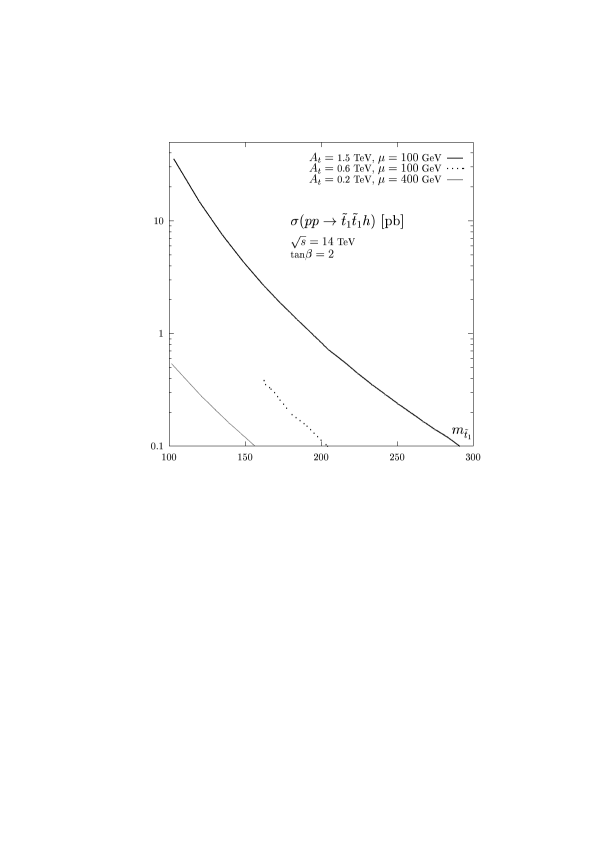
Figure 8: The production cross section $\sigma(pp\rightarrow\tilde{t}_{1}\tilde{t}_{1}h$) [in pb] as a function of the $\tilde{t}_{1}$ mass and three sets of $A_{t}$ and $\mu$ values and $\mbox{tan}\beta$ is fixed to $\mbox{tan}\beta=2$.

In Fig. 9, we fix the lightest top squark mass to $m_{\tilde{t}_{1}}=165$ GeV $\sim m_{t}^{\rm\overline{MS}}$ and display the $pp\rightarrow gg+q\bar{q}\rightarrow\tilde{t}_{1}\tilde{t}_{1}h$ cross section as a function of $\tilde{A}_{t}$. For comparison, the $*$ and $\bullet$ give the standard–like $pp\rightarrow\bar{t}th$ cross section for $M_{h}=100$ GeV and $\mbox{tan}\beta=2$ and 30, respectively. For $\mbox{tan}\beta=30$ the cross section is somewhat smaller than for $\mbox{tan}\beta=2$, a mere consequence of the increase of the $h$ boson mass with $\mbox{tan}\beta$ [49]. As can be seen again, the production cross section is substantial for the no–mixing case, rather small for intermediate mixing [becoming negligible for $\tilde{A}_{t}$ values between 200 and 400 GeV], and then becomes very large exceeding the reference cross section for values of $\tilde{A}_{t}$ above $\sim 1$ TeV. For instance, for the inputs of Fig. 8, $\sigma(pp\rightarrow\tilde{t}_{1}\tilde{t}_{1}h)$ exceeds $\sigma(pp\rightarrow t\bar{t}h)$ in the SM for the same Higgs boson mass when $\tilde{A}_{t}\raisebox{-3.69899pt}{~{}\shortstack{$>$ \\ [-0.07cm] $\sim$}}~{}1(1.05)$ TeV for $\mbox{tan}\beta=2(30)$.

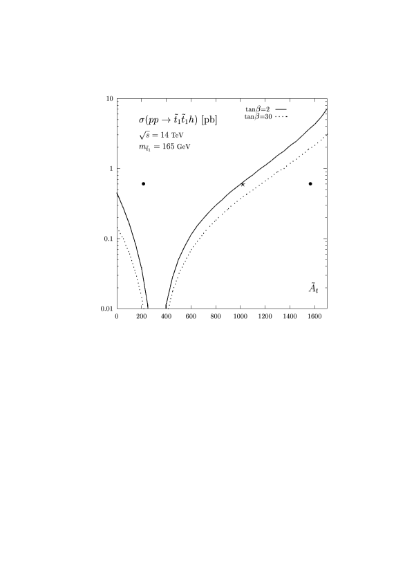
Figure 9: The production cross section $\sigma(pp\rightarrow\tilde{t}_{1}\tilde{t}_{1}h$) [in pb] as a function as a function of $\tilde{A}_{t}$ for fixed $m_{\tilde{t}_{1}}=165$ GeV and for $\mbox{tan}\beta=2,30$ (b).

For the signal, in most of the parameter space, the stop decay is $\tilde{t}_{1}\rightarrow b\chi^{+}$, if $m_{\tilde{t}_{1}}<m_{t}+m_{\chi_{1}^{0}}$ where $\chi_{1}^{0}$ is the LSP, or $\tilde{t}_{1}\rightarrow t\chi_{1}^{0}$, in the opposite case [see section 5.4]. In the interesting region where $\sigma(pp\rightarrow\tilde{t}_{1}\tilde{t}_{1}h)$ is large, i.e. for light $\tilde{t}_{1}$, the decay $\tilde{t}_{1}\rightarrow b\chi^{+}$ is dominant, unless $m_{\tilde{t}_{1}}-m_{\chi_{1}^{+}}$ is very small, in which case the loop induced decay, $\tilde{t}_{1}\rightarrow c\chi^{0}_{1}$, can become competitive. Assuming that sleptons are heavier than the chargino, $\chi_{1}^{+}$ will mainly decay into $bW^{+}+\ {\rm missing\ energy}$ leading to $\tilde{t}_{1}\rightarrow bW^{+}$ final states. This is the same topology as the decay, $t\rightarrow bW^{+}$, except that in the case of the $\tilde{t}$ there is a large amount of missing energy. If sleptons are also relatively light, charginos decays will also lead to $l\nu\chi_{1}^{0}$ final states. The only difference between the final states generated by the $\tilde{t}\tilde{t}h$ and $t\bar{t}h$ processes, will be due to the softer energy spectrum of the charged leptons coming from the chargino decay in the former case, because of the energy carried by the invisible LSP.

The Higgs boson can be tagged through its $h\rightarrow\gamma\gamma$ decay mode. In the decoupling limit, and for light top squarks and large $\tilde{A}_{t}$ values, the branching ratio for this mode can be substantially enhanced compared to the SM Higgs boson as discussed in the previous subsection. Therefore, $\gamma\gamma$+ charged lepton events can be more copious than in the SM, and the contributions of the $pp\rightarrow\tilde{t}\tilde{t}h$ process to these events can render the detection of the $h$ boson much easier than with the process $pp\rightarrow t\bar{t}h$ alone.

Although a detailed Monte–Carlo analysis will be required to assess the importance of this signal and to optimize the cuts needed not to dilute the contribution of the $\tilde{t}\tilde{t}h$ final states, it is clear that in a substantial area of the MSSM parameter space, the contribution of the top squark to the $\gamma\gamma l^{\pm}$ signal can significantly enhance the potential of the LHC to discover the lightest MSSM Higgs boson in this channel. This would be a new and very interesting means to search for top squarks at the LHC, which due to the large QCD background from $\bar{t}t$ production, are otherwise difficult to detect in other channels. Last but not least, and as welcome bonus, this process would allow to measure the $h\tilde{t}\tilde{t}$ coupling, the potentially largest electroweak coupling in the MSSM, opening thus a window to probe directly the trilinear part of the soft–SUSY breaking scalar potential.

4.2 Higgs boson decays into SUSY particles

4.2.1 SUSY decays of the neutral Higgs bosons

As discussed previously, in mSUGRA scenarii the MSSM Higgs bosons $H,A,H^{\pm}$ are rather heavy and degenerate in mass, while the lightest $h$ boson is in the decoupling regime. We have seen in the previous section 4.1 that the search of the $h$ boson at the LHC relies heavily on the rare $h\rightarrow\gamma\gamma$ decay mode, while the almost only possibility of detecting the heavy $H,A$ bosons for masses beyond 300 GeV and large enough $\mbox{tan}\beta$ values, $\mbox{tan}\beta\raisebox{-3.69899pt}{~{}\shortstack{$>$ \\ [-0.07cm] $\sim$}}~{}5$, would be to look for the decays into tau pairs, $H/A\rightarrow\tau^{+}\tau^{-}$. With high enough luminosity, these signals will be visible at the LHC [see Fig. 4].

However, in these analyses, it is always assumed that the heavy $H/A$ bosons decay only into standard particles, and that the SUSY decay modes are shut. But for such large values of $M_{H,A}$, at least the decays into the lightest neutralinos and charginos, and possibly into to light $\tilde{t}$ and $\tilde{b}$, can be kinematically allowed. These modes could have large decays widths, and thus could suppress the $H/A\rightarrow\tau^{+}\tau^{-}$ branching ratios drastically. For the $h$ boson, because of its small mass, only a little room is left for decays into SUSY particles by present experimental data [55]. However, the possibility of $h$ decays into neutralinos is not yet completely ruled out, especially if one relaxes the gaugino mass unification; decays into sneutrinos are also still possible. When these invisible decays occur, they can be dominant, hence reducing the probability of the $h\rightarrow\gamma\gamma$ decay to occur. These SUSY decays should therefore not be overlooked as they might jeopardize the detection of the Higgs particles at the LHC.

a) Invisible decays of the h boson

Despite the lower bound of $91\,$GeV on the mass of the lightest chargino $\chi_{1}^{+}$ and the constraints from $\chi_{0}^{1}\chi_{0}^{2}$ searches at LEP2 [55], the decay of the lightest $h$ boson into a pair of lightest neutralinos is still kinematically possible. Even in the constrained MSSM with a common gaugino mass at the GUT scale, leading to the well–know relation between the wino and bino masses $M_{1}=\frac{5}{3}{\rm tg}^{2}\theta_{W}M_{2}\sim\frac{1}{2}M_{2}$, the lower bound on the LSP mass is only $m_{\chi_{0}^{1}}\raisebox{-3.69899pt}{~{}\shortstack{$>$ \\ [-0.07cm] $\sim$}}~{}40$ GeV [55]. Since the upper bound on the lightest $h$ boson in the MSSM is $M_{h}\sim 130$ [49], there is still room for the invisible decay $h\rightarrow\chi_{0}^{1}\chi_{0}^{1}$ to occur.

Although high values of $\mbox{tan}\beta$ are required to be closer to the upper bound of $M_{h}$, the $hb\bar{b}$ coupling is SM–like if the $h$ boson is in the decoupling regime: in this case the $h\chi_{0}^{1}\chi_{0}^{1}$ coupling can be much larger then the $hb\bar{b}$ Yukawa coupling and the decay of the $h$ boson into the lightest neutralinos can be dominant, resulting in a much smaller BR($h\rightarrow\gamma\gamma$) than in the SM. Far from the decoupling limit, the coupling $g_{hbb}\sim\tan\beta$ is strongly enhanced for $\mbox{tan}\beta\raisebox{-3.69899pt}{~{}\shortstack{$>$ \\ [-0.07cm] $\sim$}}~{}3$, while the $h$ boson couplings to $W$ bosons and top quarks [which provide the main contributions to the $h\gamma\gamma$ loop vertex] are suppressed. This again will result in a strong suppression of BR($h\rightarrow\gamma\gamma$).

The partial width for the decay $h\rightarrow\chi_{0}^{1}\chi_{0}^{1}$ is given by [$\beta_{\chi}^{2}=1-4m^{2}_{\chi_{1}^{0}}/M_{h}^{2}$ and the coupling $g_{h\chi\chi}$ is given in eq. (3.52) of section 3.1]

$$\Gamma(h\rightarrow\chi_{0}^{1}\chi_{0}^{1})=\frac{G_{F}M_{W}^{2}M_{h}}{2\sqrt{2}\pi}\ g^{2}_{h\chi\chi}\ \beta^{3}_{\chi}$$ (4.7)

The decay is important only for moderate values of $M_{2}$ and $\mu$ [with a preference for $\mu>0$] since the $h$ boson prefers to couple to neutralinos which are a mixture of gauginos and higgsinos. In this range, the decay $h\rightarrow\chi_{0}^{1}\chi_{0}^{1}$ is dominant if $M_{h}$ is above the $2m_{\chi_{0}^{1}}$ threshold; close to the threshold, the decay width is strongly suppressed by the $\beta^{3}_{\chi}$ factor.

As an illustration of this possibility we show in Fig. 10 the fraction BR$(h\rightarrow\gamma\gamma)$ as a function of $\mu$ for two values of $\mbox{tan}\beta=2,30$. We choose $M_{A}=1$ TeV [to be in the decoupling regime] and the “maximal mixing” scenario $A_{t}=\sqrt{6}m_{\tilde{q}}$ with the common squark mass parameter fixed to 1 TeV [to maximize the $h$ boson mass]; this gives $M_{h}\simeq 126$ GeV for $\mbox{tan}\beta=30$ and $M_{h}\simeq 106$ GeV for $\mbox{tan}\beta=2$ [the variation with $\mu$ is almost negligible]. Focusing first on the $\tan\beta=30$ and $M_{2}=140$ GeV case, for $|\mu|\raisebox{-3.69899pt}{~{}\shortstack{$>$ \\ [-0.07cm] $\sim$}}~{}200$ GeV the channel $h\rightarrow\chi_{1}^{0}\chi_{1}^{0}$ is kinematically closed and the $\gamma\gamma$ branching ratio is SM–like, BR $\simeq 2.3\times 10^{-3}$. In the range $110\raisebox{-3.69899pt}{~{}\shortstack{$<$ \\ [-0.07cm] $\sim$}}~{}|\mu|\raisebox{-3.69899pt}{~{}\shortstack{$<$ \\ [-0.07cm] $\sim$}}~{}200$ GeV, the LSP is lighter that $M_{h}/2$ while the chargino is still heavier than 91 GeV, the decay $h\rightarrow\chi_{1}^{0}\chi_{1}^{0}$ is thus allowed to occur and suppresses the $\gamma\gamma$ branching ratio. The suppression is stronger with decreasing $|\mu|$ since on the one hand the phase-space becomes more favorable, and on the other hand the LSP tends to be an equal mixture of higgsino and gaugino. The maximum drop of BR($h\rightarrow\gamma\gamma$) is a factor of three and two for $\mu>0$ and $\mu<0$ respectively. For values $|\mu|\raisebox{-3.69899pt}{~{}\shortstack{$<$ \\ [-0.07cm] $\sim$}}~{}110$ GeV, $m_{\chi_{1}^{\pm}}$ exceeds its experimentally allowed lower bound.

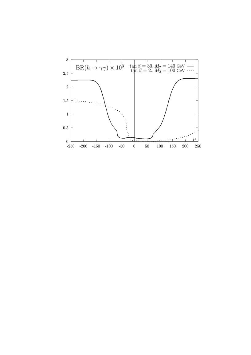
Figure 10: Branching ratios in units of $10^{-3}$ for the decays $h\rightarrow\gamma\gamma$ as a function of $\mu$ for $\mbox{tan}\beta=2(30)$ and $M_{2}=100(140)$ GeV.

In the case $\mbox{tan}\beta=2$ and $M_{2}=100$ GeV, the only experimentally allowed region is $|\mu|\raisebox{-3.69899pt}{~{}\shortstack{$>$ \\ [-0.07cm] $\sim$}}~{}110$ GeV with $\mu<0$, since elsewhere the chargino is heavier than 91 GeV. In this $|\mu|$ range, the decay $h\rightarrow\chi_{1}^{0}\chi_{1}^{0}$ is kinematically allowed, but the branching ratio is very small, less than 0.5%. This is due to the fact that in this area $\chi_{0}^{1}$ is a pure bino state and its couplings to the $h$ boson are strongly suppressed. What makes the $h\rightarrow\gamma\gamma$ branching ratio drop by almost a factor two compared to the previous case is first, the smaller mass of the $h$ boson [the decay width grows with the third power of the Higgs mass] but also because of the contribution of the chargino loops to the $h\rightarrow\gamma\gamma$ decay which interfere destructively for $\mu<0$ with the dominant contribution due $W$ loops [the reduction is nevertheless very mild, at most 15% in this case].

If the constraint on the unification of the gaugino masses at the GUT scale is relaxed, there is practically no lower bound on the LSP mass. Indeed, for relatively large values of the Higgs–higgsino mass parameter $\mu$, the lightest chargino $\chi_{1}^{+}$ and the next–to–lightest neutralino $\chi_{2}^{0}$ are wino–like with a mass $\sim M_{2}$ while the lightest neutralino is bino–like with a mass $\sim M_{1}$. Since $M_{1}$ is a free parameter, it can be as small as possible leading to a possibly very light LSP. The decay $h\rightarrow\chi_{0}^{1}\chi_{0}^{1}$ will then have more room to occur.

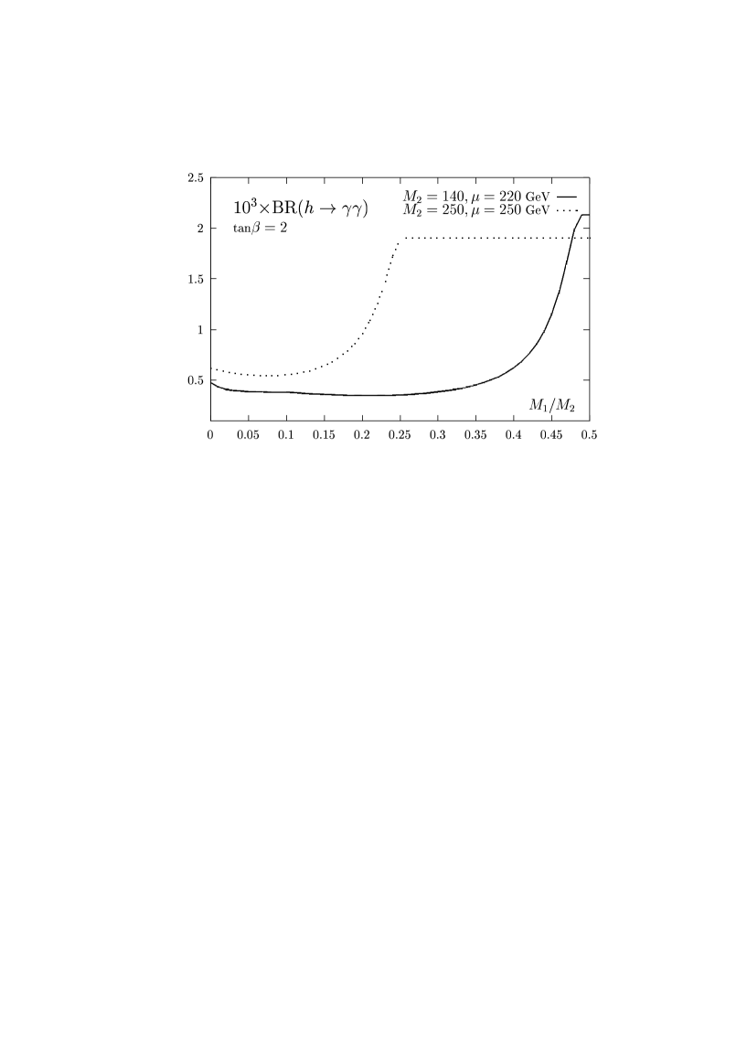
Figure 11: Branching ratios for the decays $h\rightarrow\gamma\gamma$ in units of $10^{-3}$ as a function of $M_{1}/M_{2}$ for $\mbox{tan}\beta=2$ and two sets of $M_{2},\mu$ values.

The branching ratio for the decay $h\rightarrow\chi_{1}^{0}\chi_{1}^{0}$ can be rather large thus suppressing the $\gamma\gamma$ branching ratio. This is exemplified in Fig. 11, where BR($h\rightarrow\gamma\gamma$) is shown as a function of the ratio $M_{1}/M_{2}$ for $\mbox{tan}\beta=2$ and for two sets of $M_{2}$ and $\mu$ values; $M_{2}=140$ GeV, $\mu=220$ GeV leading to $m_{\chi_{1}^{+}}\simeq 96$ GeV, and $M_{2}=\mu=250$ GeV leading to $m_{\chi_{1}^{+}}\simeq 175$ GeV; the remaining inputs are as in the previous figure. In the first scenario [solid lines], when the LSP is very small BR$(h\rightarrow\gamma\gamma$) drops to the level of $5.10^{-4}$, a strong reduction compared to the expected rate $\sim 2.10^{-3}$. With increasing $M_{1}/M_{2}$ and hence with increasing LSP mass, it stays almost constant until the $2m_{\chi_{1}^{0}}$ threshold is reached for $M_{1}\sim M_{2}/2$ and the branching ratio recovers its standard value.

In the second scenario [dotted lines], BR($h\rightarrow\gamma\gamma$) starts at the same level as previously, but increases more rapidly and reaches approximately the standard value for $M_{1}\sim M_{2}/4$ which corresponds to the kinematical limit for the decay $h\rightarrow\chi_{1}^{0}\chi_{1}^{0}$. When the LSP decay is shut, the difference between the $\gamma\gamma$ branching ratios in the two scenarios is due to a constructively interfering chargino loop contribution [the sign of the $\chi_{1}^{\pm}$ contribution goes with the sign of $\mu$] in the case where $m_{\chi_{1}^{+}}\simeq 96$ GeV and which enhances the $\gamma\gamma$ decay width by 20% or so. This picture is expected not to be altered significantly for larger values of $\mbox{tan}\beta$ if the $h$ boson is in the decoupling regime as discussed previously [in fact for large $\mbox{tan}\beta$ values and for some moderate values of the parameters $M_{2}$ and $\mu$, even the decays into the lightest and the next to lightest neutralinos is possible].

Another kinematically still possible SUSY mode for the lightest $h$ boson is the decay into sneutrinos. Indeed, the experimental lower bound on the $\tilde{\nu}$ masses is still rather low, $m_{\tilde{\nu}}\raisebox{-3.69899pt}{~{}\shortstack{$>$ \\ [-0.07cm] $\sim$}}~{}45$ GeV [55], leaving some room for the decay $h\rightarrow\tilde{\nu}\tilde{\nu}$ to occur. However, because of SU(2)_L invariance, the sneutrino and the left–handed charged slepton masses are related and one should avoid being into conflict with the experimental bounds on the $\tilde{l}_{L}$ mass which are stronger, $m_{\tilde{l}_{L}}\raisebox{-3.69899pt}{~{}\shortstack{$>$ \\ [-0.07cm] $\sim$}}~{}70$ GeV. However, even in this case one can obtain a rather light sneutrino since a splitting between the $\tilde{\nu}$ and $\tilde{l}_{L}$ masses can be generated by the D–terms. Indeed, recalling eqs. (3.39) and denoting the common scalar mass by $\tilde{m}$, one has:

$$m_{\tilde{\nu}}^{2}\simeq\tilde{m}^{2}+0.50M_{Z}^{2}\cos 2\beta\ \ ,\ \ m_{\tilde{l}_{L}}^{2}\simeq\tilde{m}^{2}-0.27M_{Z}^{2}\cos 2\beta$$ (4.8)

For small values of $\tilde{m}$, the slepton masses are governed by the D–terms, and for large values of $\mbox{tan}\beta$, $\cos 2\beta\rightarrow-1$ and the D–terms become maximal. Since they tend to increase $m_{\tilde{l}_{L}}$ and decrease $m_{\tilde{\nu}}$, relatively low masses for sneutrinos can be kept while still having rather heavy left–handed sleptons [note however, that the $\tilde{\nu}$ should not be lighter than the lightest neutralino which is expected to be the LSP].

In the decoupling limit, the $h$ boson coupling to sneutrinos is also proportional to $\cos 2\beta$ [eq. (3.51) of section 3.1], and for large $\mbox{tan}\beta$ values it becomes also maximal. And since it is a “gauge” coupling, it is much larger than the $hb\bar{b}$ Yukawa coupling, and the decay $h\rightarrow\tilde{\nu}\tilde{\nu}$ is always largely dominating once it is kinematically allowed. The partial decay width for the decay, summing over the three sneutrinos, is given by

$$\Gamma(h\rightarrow\tilde{\nu}\tilde{\nu})=\frac{3G_{F}M_{Z}^{4}}{8\sqrt{2}\pi M_{h}}\beta_{\tilde{\nu}}\ \ ,\ \ \beta_{\tilde{\nu}}=\left[1-\frac{4m^{2}_{\tilde{\nu}}}{M_{h}^{2}}\right]^{1/2}$$ (4.9)

Modulo the velocity factor $\beta_{\tilde{\nu}}$, the partial width is larger than the otherwise dominant $b\bar{b}$ decay width by a huge factor: $M_{Z}^{4}/(2m_{b}^{2}M_{h}^{2})\sim 230$ for $M_{h}=130$ GeV. Thus, if the $h\rightarrow\tilde{\nu}\tilde{\nu}$ decay mode is allowed, all the branching ratios for the other decay channels including the $h\rightarrow\gamma\gamma$ mode, will be suppressed by two orders of magnitude! Since the sneutrinos will decay invisibly in this mass range [$m_{\tilde{\nu}}<m_{\chi_{1}^{\pm}}$ and the only possible mode is $\tilde{\nu}\rightarrow\nu\chi_{1}^{0}$], the $h$ boson would be then also very difficult to detect at the LHC.

b) H/A decays into SUSY particles

If the CP–even and the CP-odd Higgs bosons $H$ and $A$ are heavy, $M_{H,A}\raisebox{-3.69899pt}{~{}\shortstack{$>$ \\ [-0.07cm] $\sim$}}~{}300$ GeV, at least the decays into the lightest neutralinos and possibly charginos should be kinematically allowed. If the couplings to $b\bar{b}$ and $\tau^{+}\tau^{-}$ pairs [which together with $t\bar{t}$ states account for most of the total decay width in the absence of SUSY modes] are not strongly enhanced, and hence for not too large values of $\tan\beta$, these decays might be dominant and suppress drastically the branching ratios for the $H/A\rightarrow\tau^{+}\tau^{-}$ signals. This is exemplified in Fig. 12 where BR$(H/A\rightarrow\tau^{+}\tau^{-})$ are plotted as a function of the $H/A$ masses for three values $\mbox{tan}\beta=5,10$ and 30. The choice $M_{2}=-\mu=200$ GeV has been made leading to $m_{\chi_{1}^{0}}\sim 90$ GeV and $m_{\chi_{1}^{+}}\sim 160$ GeV [with a small variation with $\mbox{tan}\beta$].

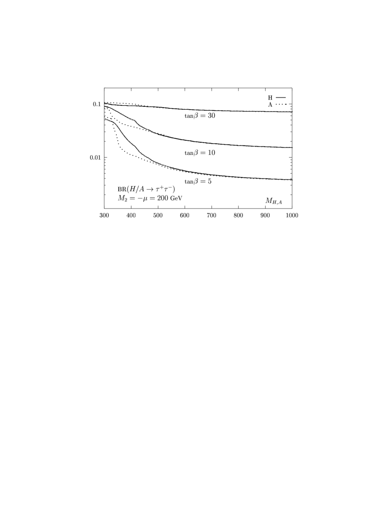
Figure 12: Branching ratios for the decays $H/A\rightarrow\tau^{+}\tau^{-}$ as a function of $M_{H,A}$ for $\mbox{tan}\beta=5,10$ and 30 and for the values $M_{2}=-\mu=200$ GeV.

The branching ratios for $H$ and $A$ decays are almost the same except for small values of $\mbox{tan}\beta$ and relatively small Higgs masses: in this case, the decoupling limit is not yet reached and additional [and different] decay modes occur for the $H$ and $A$ bosons; see section 4.1. For $\mbox{tan}\beta=5$ the $H/A$ couplings to down–type fermions are not very strongly enhanced and the decays into charginos and neutralinos have large branching ratios: they decrease BR$(H/A\rightarrow\tau^{+}\tau^{-})$ from the standard $\sim 10\%$ value for small Higgs masses [where only a few SUSY channels are open and some are suppressed by phase space] to less than 0.4% for very heavy Higgs boson masses $M_{H,A}\sim 1$ TeV [here most of the neutralino/chargino channels are open and they are not suppressed by phase space], thus a reduction by more than a factor of 20 compared to the branching ratio without the SUSY decays. For $\mbox{tan}\beta=10$, the couplings to $b$–quarks and $\tau$–leptons are more enhanced and BR$(H/A\rightarrow\tau^{+}\tau^{-})$ are larger by slightly more than a factor two compared to the previous case. For even larger values of $\mbox{tan}\beta$, $\mbox{tan}\beta=30$, the decays into charginos and neutralinos are not dominating anymore, and the branching ratios for the $H/A$ decays into tau pairs are suppressed only slightly, less than a factor of two. The branching ratios for the decays into $\mu^{+}\mu^{-}$ can be obtained from Fig. 12 by rescaling the numbers by $m_{\mu}^{2}/m_{\tau}^{2}$.

In the preceding discussion, the decays of the $H$ and $A$ bosons into sfermions were assumed to be shut. However, as discussed previously, at least one of the stops can be rather light and its couplings to the Higgs bosons enhanced; the decays of the heavier Higgs bosons $H,A$ to stop squarks might be therefore kinematically accessible and could dominate over the standard decays, and even over the decays into charginos and neutralinos. Indeed, in the decays of the $H$ boson into stops, the partial widths up to mixing angle factors are proportional to $G_{F}m_{t}^{4}/(M_{H}\tan^{2}\beta)$ or/and $G_{F}m_{t}^{2}(\mu-A_{t}/\mbox{tan}\beta)^{2}/M_{H}$; for small $\mbox{tan}\beta$ values and not too large $M_{H}$ and for intermediate $\mbox{tan}\beta$ values and for large $\mu$ and $A_{t}$, the widths for the decays $H\rightarrow\tilde{t}\tilde{t}$ can be very large and can compete with, and even dominate over, the other [standard and SUSY] decay channels. The branching ratios for the $H$ decays into $\tau$ pairs would be then further suppressed.

,

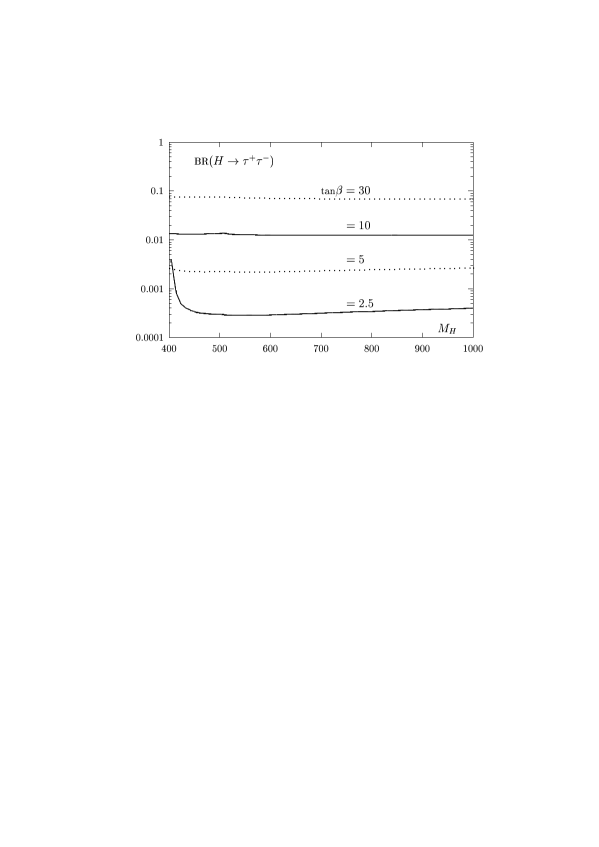
Figure 13: Branching fractions for $H\rightarrow\tilde{t}_{1}\tilde{t}_{1}$ [left] and $H\rightarrow\tau^{+}\tau^{-}$ [right] as a function of $M_{H}$ for $\mbox{tan}\beta=2.5,5,10,30$ and $M_{2}=\mu=m_{\tilde{f}}/2=250$ GeV and $A_{t}=1.5$ TeV.

This is illustrated in Fig. 13, where BR$(H\rightarrow\tilde{t}_{1}\tilde{t}_{1}$) is shown as a function of $M_{H}$ for $\mbox{tan}\beta=2.5,5,10,30$ and $m_{\tilde{t}_{1}}\simeq 200$ GeV [for $\mbox{tan}\beta=2.5$ this is achieved by setting $m_{\tilde{f}_{L}}=m_{\tilde{f}_{R}}=500$ GeV and $A_{t}=1.5$ TeV]; $M_{2}=\mu=250$ GeV. As expected BR$(H\rightarrow\tilde{t}_{1}\tilde{t}_{1}$) decreases with increasing $\mbox{tan}\beta$ values and increasing $M_{H}$. However, it is still at the level of $\sim 50\%$ for $\mbox{tan}\beta=5$ and $M_{H}=1$ TeV. For $\mbox{tan}\beta=30$, the channel $H\rightarrow\tilde{t}_{1}\tilde{t}_{2}$ opens up for $M_{H}\sim 900$ GeV, and the curve shows the sum BR$(H\rightarrow\tilde{t}_{1}\tilde{t}_{1}+\tilde{t}_{1}\tilde{t}_{2}$). But for this large $\mbox{tan}\beta$ value, the branching ratio barely exceeds the level of $20\%$ in contrast to lower $\mbox{tan}\beta$ values where it can reach almost unity for small $M_{H}$. For larger $M_{H}$, the decays into charginos and neutralinos become more important and will dominate; so BR$(H\rightarrow\tau^{+}\tau^{-})$ is reduced anyway. For the $A$ boson the only important decay into sfermions is $A\rightarrow\tilde{t}_{1}\tilde{t}_{2}$ [and maybe $\tilde{b}_{1}\tilde{b}_{2}$ for $\mbox{tan}\beta\gg 1$]. Thus both stops must be light for the decay to be allowed by kinematics. This happens only in a small area of the parameter space, unless all squarks are relatively light. For instance, in the scenario of Fig. 13, $m_{\tilde{t}_{2}}\sim 700$ GeV and the decays $A,H\rightarrow\tilde{t}_{1}\tilde{t}_{2}$ occur only for masses close to 1 TeV.

4.2.2 Decays of the charged bosons

Charged Higgs bosons are searched for at the Tevatron and will be searched for at the LHC in the mass range $M_{H^{\pm}}<m_{t}-m_{b}$, i.e. when produced by a decaying $t$–quark. Some experimental limits from Tevatron [a $\mbox{tan}\beta$–$M_{H^{\pm}}$ exclusion contour] are already available [76]. However, the detection techniques rely on the assumption that no $H^{+}$ decay mode other than $c\bar{s}$ and $\tau^{+}\nu_{\tau}$ is kinematically significant, and in particular that no decay into SUSY particles is possible. However, decays into the lightest charginos and neutralinos as well as decays into sleptons [10] are still allowed by present experimental data; for instance, the decay channel $H^{+}\to\chi_{1}^{+}\chi_{1}^{0}$ is certainly possible for $M_{H^{\pm}}\raisebox{-3.69899pt}{~{}\shortstack{$>$ \\ [-0.07cm] $\sim$}}~{}130\,$GeV, despite the lower bound of $m_{\chi_{1}^{+}}\geq 91$ GeV [55].

In Fig. 14a, the relative branching ratio for the decay $H^{+}\to\chi_{1}^{+}\chi_{1}^{0}$ is shown as a function of $M_{H^{+}}$, for $\mbox{tan}\beta=2$, $M_{2}=110\,$GeV, $|\mu|=500\,$GeV, and all remaining soft masses large enough to forbid other supersymmetric decay modes. For these values of parameters, one has $m_{\chi_{1}^{+}}=96.5\,$GeV and $m_{\chi_{1}^{0}}\simeq 50\,$GeV. Also shown is the case where the assumption of gaugino mass universality is relaxed: keeping fixed all other parameters to the previous values, $M_{1}$ is set to $20\,$GeV, and the lightest neutralino mass becomes $m_{\chi_{1}^{0}}\simeq 16\,$GeV. In this case, the decay channel $\chi^{+}_{1}\chi^{0}_{1}$ opens already at $\sim 115\,$GeV. For small values of $\mbox{tan}\beta$, whenever kinematically allowed, the mode $\chi_{1}^{+}\chi_{1}^{0}$ is the dominant one. For large values of $\mbox{tan}\beta$, however, only the channel $H^{+}\to\tau^{+}\nu_{\tau}$ survives.

,

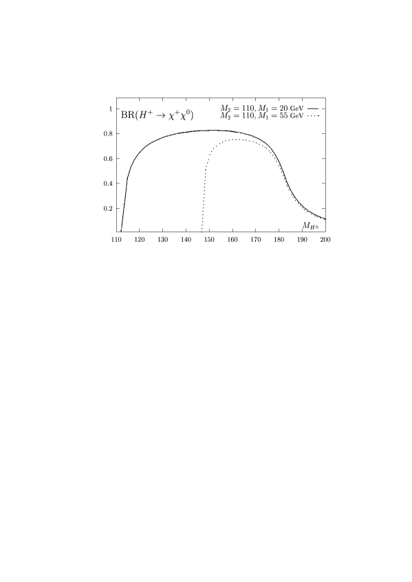
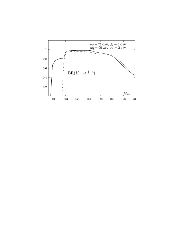
Figure 14: Branching fractions for the decays $H^{+}\to\chi_{1}^{+}\chi_{1}^{0}$ (left) and $H^{+}\to\tilde{l}^{+}\tilde{\nu}$ (right) as a function of $M_{H^{\pm}}$, for $\mbox{tan}\beta=2$, and some $M_{2},M_{1},\mu$ and $A$ values.

The previous discussion applies only to supersymmetric models with heavy sfermion masses. The existing lower bounds on slepton masses, however, are still rather modest: $\sim 65$ GeV for $\tilde{\tau}$’s and $\raisebox{-3.69899pt}{~{}\shortstack{$>$ \\ [-0.07cm] $\sim$}}~{}\,45$ GeV for $\tilde{\nu}$’s [55]. The decay $H^{+}\to\tilde{\tau}^{+}\tilde{\nu}_{\tau}$ is therefore kinematically possible for $M_{H^{\pm}}\raisebox{-3.69899pt}{~{}\shortstack{$>$ \\ [-0.07cm] $\sim$}}~{}110$ GeV. Fig. 14b shows the relative branching ratio for $\mbox{tan}\beta=2$, $M_{2}=120\,$GeV, $M_{1}\sim M_{2}/2$ and two choices of parameters in the slepton mass matrices: (a) $m_{\tilde{l}_{L}}=m_{\tilde{l}_{R}}=m_{\tilde{l}}=75\,$GeV, $\mu=500\,$GeV, $A_{\tau}=0$ and (b) $m_{\tilde{l}}=90\,$GeV, $\mu=-500\,$GeV, $A_{\tau}=1\,$TeV. This leads to a slepton spectrum: $(a)$ $m_{\tilde{\nu}}=56$ GeV, $m_{\tilde{e}}\sim m_{\tilde{\mu}}=83$ GeV and the two $\tilde{\tau}$ masses are 10 GeV below and above this value, and $(b)$ $m_{\tilde{\nu}}=75\,$GeV, $m_{\tilde{e}}\sim m_{\tilde{\mu}}=97\,$GeV and $m_{\tilde{\tau}_{1}}=63\,$GeV, and $m_{\tilde{\tau}_{2}}=121\,$GeV.

The prominence of the $H^{+}\rightarrow\tilde{\tau}^{+}\tilde{\nu}_{\tau}$ mode above threshold is explained by the fact that the $H^{+}\tilde{\nu}_{L}^{*}\tilde{l}_{L}$ coupling $\propto g/\sqrt{2}M_{W}\sin 2\beta$ is very large compared to the $H^{+}{\nu}_{L}^{*}{\tau}_{R}$ coupling $g/\sqrt{2}(m_{\tau}/M_{W})$. Due to the $\sin 2\beta$ dependence, this term quickly dies off for increasing $\tan\beta$. In this case, however, there exists other directions of parameter space where this decay mode has still a branching ratio close to unity. When $A_{\tau}\sim\mu\mbox{tan}\beta$, in fact, the left–right mixing in the slepton mass matrix tends to vanish, but the coupling of the Lagrangian term $H^{+}\tilde{\nu}_{L}^{*}\tilde{\tau}_{R}$: $-g/\sqrt{2}(m_{\tau}/M_{W})(\mu+A_{\tau}\mbox{tan}\beta)$ acquires a $1/\cos^{2}\beta$ dependence, which increases with increasing $\mbox{tan}\beta$. For instance, $\mbox{tan}\beta=10$, $A_{\tau}=2\,$TeV, $\mu\sim 200\,$GeV and $m_{l}\sim 80\,$GeV, give a branching ratio above $90\%$ for the decay channel $H^{+}\to\tilde{\tau}^{+}\tilde{\nu}_{\tau}$, when kinematically accessible. Such a decay mode produces a final $\tau^{+}$ plus missing energy as the $\tau^{+}\nu_{\tau}$ mode, but with a much softer $\tau^{+}$ than that searched for at hadron colliders.

Finally, let us make a few remarks on other possible decay of $H^{\pm}$ in non–SUSY two–Higgs doublet models (2HDM). Although the decay $b\to s\gamma$ excludes masses $M_{H^{\pm}}$ up to $\sim 165\,$GeV, irrespectively of $\tan\beta$ [77], direct searches still allow for the possibility $M_{H^{\pm}}<M_{W}$. The $H^{\pm}$ states are searched for at LEP2 and the Tevatron, relying again on the $c\bar{s}$ and $\tau\nu$ signals [see Ref. [10] for details and references].

$(i)$ In 2HDMs, there is no lower bound on the pseudoscalar mass $M_{A}$ coming from LEP: since the mixing angle $\alpha$ is in this case a free parameter, it can be chosen in such a way that the coupling $ZhA$ vanishes and the process $Z\to hA$ does not occur. This makes that the LEP2 bound $M_{A}>75$ GeV [55] does not hold, leaving open the possibility of a very light $A$ boson. [In this case the cross section for the process $e^{+}e^{-}\to Z^{*}\to hZ$, which is complementary, is not suppressed compared to the SM Higgs boson, and the bound $M_{h}>88.6\,$GeV [55] applies here]. Now since $g_{H^{+}W^{-}A}$ is a “gauge” coupling, it is clear that the decay $H^{+}\to AW^{+}$ can be rather important in a 2HDM. Indeed, this remains true even for an off–shell $W$–boson, in spite of the virtuality and the additional weak coupling suppressions. Even for masses $M_{H^{\pm}}\sim 55$ GeV, i.e. roughly the value excluded at LEP2, the branching ratio can be still at the level of 50% for small enough $\mbox{tan}\beta$ and $M_{A}$ values. For heavier $H^{\pm}$ bosons that can be searched for at the Tevatron, the decay $H^{\pm}\rightarrow AW^{(*)}$ can be by far the dominant one.

$(ii)$ For charged Higgs boson masses above $\sim 140$ GeV, even if the decays into $AW^{*}$ bosons are suppressed [for instance the $A$ boson is too heavy], the $H^{+}\to\tau\nu_{\tau}$ and $c\bar{s}$ channels are still not the dominant ones for small $\mbox{tan}\beta$ values. Indeed, for $\mbox{tan}\beta\sim 1$ the three–body decay mode $H^{+}\to\bar{b}t^{*}\to\bar{b}bW^{+}$ is already the dominant decay mode: despite the virtuality of the top quark and the fact that the process is of higher–order, the $H^{\pm}$ coupling to $tb$ quarks is much larger than the $\tau\nu$ and $cs$ couplings, leading to a large compensation. For instance, for $M_{H^{\pm}}=140$ GeV and $\mbox{tan}\beta=1$, the branching ratio is already at the level of 50%. Note that this decay mode [as well as the three–body decay mode $H^{\pm}\rightarrow hW^{*}\rightarrow hf\bar{f}$] can also be important in the MSSM for large enough $H^{\pm}$ masses [but still below $m_{t}-m_{b}$] and small $\mbox{tan}\beta$ values.

4.3. MSSM Higgs production in $e^{+}e^{-}$ collisions

4.3.1 Production mechanisms

The main production mechanisms of the neutral MSSM Higgs bosons at $e^{+}e^{-}$ colliders are the Higgs–strahlung process and pair production [79, 80], as well as the $WW$ and $ZZ$ fusion processes [68]:

$$(a)\ \ {\rm Higgs\mbox{-}strahlung}\hskip 28.45274pte^{+}e^{-} \rightarrow (Z)\rightarrow Z+h/H\hskip 142.26378pt$$

$$(b)\ \ {\rm pair\ production}\hskip 28.45274pte^{+}e^{-} \rightarrow (Z)\rightarrow A+h/H$$

$$(c)\ \ {\rm fusion\ processes}\hskip 22.76228pt\ e^{+}e^{-} \rightarrow \bar{\nu}\nu\ (WW)\rightarrow\bar{\nu}\nu\ +h/H\hskip 99.58464pt$$

$$e^{+}e^{-} \rightarrow e^{+}e^{-}(ZZ)\rightarrow e^{+}e^{-}+h/H$$ (4.10)

The CP–odd Higgs boson $A$ cannot be produced in the Higgs–strahlung and fusion processes to leading order since it does not couple to vector boson pairs.

The charged Higgs particle [80] can be pair produced through virtual photon and $Z$ boson exchange in $e^{+}e^{-}$ collisions, and also in top-quark decays for masses below $m_{t}-m_{b}\sim 170$ GeV:

$$(d)\ \ {\rm charged\ Higgs}\hskip 22.76228pt\ e^{+}e^{-} \rightarrow \ (\gamma,Z^{*})\ \rightarrow\ H^{+}H^{-}\hskip 111.8191pt$$

$$e^{+}e^{-} \rightarrow t\bar{t}\ {\rm with}\ t\rightarrow H^{+}b$$ (4.11)

The production cross sections for the neutral Higgs bosons are suppressed by mixing angle factors compared to the SM Higgs production,

$$\sigma(e^{+}e^{-}\rightarrow Zh)\ ,\ \sigma(VV\rightarrow h)\ ,\ \sigma(e^{+}e^{-}\rightarrow AH)\ \ \sim\ \sin^{2}(\beta-\alpha)$$

$$\sigma(e^{+}e^{-}\rightarrow ZH)\ ,\ \sigma(VV\rightarrow H)\ ,\ \sigma(e^{+}e^{-}\rightarrow Ah)\ \ \sim\ \cos^{2}(\beta-\alpha)$$ (4.12)

while the cross section for the $H^{\pm}$ particles does not depend on any parameter other than $M_{H^{\pm}}$ when pair produced in $e^{+}e^{-}$ collisions; a $\mbox{tan}\beta$ dependence is however present for $H^{\pm}$ production in top decays, due to the branching ratio BR$(t\rightarrow H^{+}b)$.

Modulo the mixing factors, the cross section for the fusion process, $e^{+}e^{-}\rightarrow\bar{\nu}_{e}\nu_{e}\Phi$ with $\Phi=h,H$ is enhanced at high energies since it scales like $M_{W}^{-2}\log s/M_{\Phi}^{2}$; the cross section for $e^{+}e^{-}\rightarrow e^{+}e^{-}\Phi$ is $\sim 16\cos^{2}\theta_{W}$ i.e. one order of magnitude smaller. The cross sections for the Higgs–strahlung and pair production processes, $e^{+}e^{-}\rightarrow\Phi Z,\Phi A$ and $H^{+}H^{-}$ scale like $1/s$ and hence are smaller at high energies. Close to the decoupling limit, the factor $\cos(\beta-\alpha)\rightarrow M_{Z}^{2}\sin 2\beta/(2M_{A}^{2})$ vanishes, and the only relevant processes for the production of the heavy states [when kinematically allowed] are the pair production of $A$ and $H$ and the charged Higgs pair production: $e^{+}e^{-}\rightarrow HA$ and $e^{+}e^{-}\rightarrow H^{+}H^{-}$. The cross section for the fusion process, $e^{+}e^{-}\rightarrow\nu\bar{\nu}H$, which in principle is enhanced at high energies, is only relevant in the mass range of a few hundred GeV and for small $\mbox{tan}\beta$ values where the factor $\cos^{2}(\beta-\alpha)$ is not prohibitively small. For the lightest $h$ boson, the only remaining production processes are the bremsstrahlung and vector boson fusion mechanisms: $e^{+}e^{-}\rightarrow hZ$ and $e^{+}e^{-}\rightarrow\nu\bar{\nu}/e^{+}e^{-}+h$, exactly like for the SM Higgs bosons.

The cross sections for processes the $(a)$–$(c)$ and $(d)$ are shown in Figs. 15 and 16 as functions of the Higgs boson masses for $\mbox{tan}\beta=2.5$ at a c.m. energy $\sqrt{s}=500$ GeV. They are obtained with the help of the program HPROD to be discussed later.

There are several additional processes for the production of the neutral Higgs particles, and in particular of the lightest $h$ boson, that we will take as an example. Although these processes are of higher order, the production rates can be substantial for high–luminosities, and they might open a window to the determination of several fundamental properties of the Higgs particles.

$(i)$ The associated production with $t\bar{t}$ pairs [81] which allows to measure directly the $t\bar{t}$–Higgs Yukawa coupling, the strongest coupling in the standard sector:

$$e^{+}e^{-}\ \rightarrow\ (\gamma,Z^{*})\ \rightarrow\ t\bar{t}\Phi$$ (4.13)

$(ii)$ The double Higgs boson production, either in the bremsstrahlung or in the fusion processes, which allows to determine the trilinear Higgs boson couplings, and reconstruct the all important scalar potential [82, 83]

$$e^{+}e^{-}\rightarrow Zhh\ \ {\rm and}\ \ WW/ZZ\rightarrow hh$$ (4.14)

$(iii)$ The production of the Higgs bosons in association with a photon [84, 85], which allows to measure the $h\gamma\gamma$ and $hZ\gamma$ loop induced vertices and probe the effects of heavy particles which couple to the Higgs boson

$$e^{+}e^{-}\rightarrow h\gamma$$ (4.15)

In addition, if stop squarks are light, the production of the $h$ boson with stop pairs, $e^{+}e^{-}\rightarrow\tilde{t}\tilde{t}h$ [86], which allows to measure the $\tilde{t}\tilde{t}h$ couplings, the largest electroweak couplings in the MSSM, opening a window to the probing of trilinear couplings.

Finally, $e^{+}e^{-}$ linear colliders can be made to run in the $\gamma\gamma$ mode with the high energy photons coming from Compton back–scattering [87] of laser photons. This lead to the production of the Higgs bosons as $s$–channel resonances: $\gamma\gamma\rightarrow h,H,A$, allowing to measure the Higgs–photon couplings [similarly to the process $e^{+}e^{-}\rightarrow\gamma$+Higgs]. Furthermore charged Higgs bosons can be pair–produced in this mode.

4.3.2 The program HPROD

There are many generators which deal with the production of the MSSM Higgs bosons at $e^{+}e^{-}$ colliders [53]. Here, we briefly describe the program HPROD [11] which calculates the cross sections of the SM and MSSM Higgs particles at $e^{+}e^{-}$ machines. It includes:

$(i)$ In the SM: the strahlung and the $WW/ZZ$ fusion processes as well as the higher order processes $e^{+}e^{-}\rightarrow ttH^{0},H^{0}H^{0}Z$ and $VV\rightarrow H^{0}H^{0}$ in the longitudinal vector boson approximation. The associated production with a photon will be included soon.

$(ii)$ In the MSSM it includes all the processes $(a)$–$(d)$ above: the strahlung and the pair production as well as the $WW/ZZ$ fusion processes for neutral Higgs production, and the $e^{+}e^{-}$ and top decay processes for the charged Higgs boson. The higher order processes will be included soon.

$(iii)$ In the MSSM, the complete radiative corrections in the effective potential approach with full mixing in the $\tilde{t},\tilde{b}$ sectors; it uses the RG improved values of the masses and couplings, and the relevant leading next–to–leading–order corrections are also implemented. Both the pole and the running Higgs boson masses are calculated.

$(iv)$ Off–shell $Z$ and Higgs bosons in the bremsstrahlung and the Higgs pair production processes [the latter only in the region of parameter space where they are relevant: close to the production threshold and for sizeable Higgs boson decay widths]. The Higgs boson total widths [without the decays into SUSY particles] are included in the routines.

$(v)$ The initial state radiative corrections for the bremsstrahlung, pair production processes and the $WW/ZZ$ fusion processes. The effect of beamstralung for the TESLA machine by making an interface with the program CIRCEE [88] will be implemented soon.

The basic input parameters, fermion and gauge boson masses and their total widths, coupling constants and in the MSSM, soft SUSY–breaking parameters can be chosen from an input file. In this file several flags allow to switch on/off or change some options [e.g. choose a particular Higgs boson, include/exclude initial state radiation, use running or pole Higgs masses]. The parameters in the input file are:

$\sqrt{s}$ the c.m. energy of the collider; IHIGGS: an integer which chooses the Higgs boson [0,1,2,3 for $H^{0},h,H,H^{\pm}$ and 4 for all MSSM Higgs bosons]; $\mbox{tan}\beta$ and $M_{A}$: the two basic parameters in the MSSM Higgs sector; $m_{b},m_{t}$ the bottom and top masses; $\alpha_{s}(M_{Z}),G_{F},\alpha(0)$: the strong, Fermi and QED coupling constants; $M_{Z},M_{W},\Gamma_{Z}$: the $W,Z$ boson masses and the $Z$ total width; $M_{2},\mu,m_{\tilde{Q}_{L}},m_{\tilde{U}_{R}},m_{\tilde{D}_{R}}$: the SUSY breaking mass parameters; $A_{b},A_{t}$: SUSY breaking trilinear coupling for stops and sbottoms; ISHELZ/ISHELH: integers which for 1(0) include (exclude) off-shell $Z$/Higgs bosons in the bremsstrahlung/pair production processes; IPOLE: an integer which for 0(1) calculates running (pole) MSSM Higgs masses; ISR: an integer which for 1(0) excludes (includes) initial state radiation; IHIGH: an integer which for 0(1) includes (excludes) the higher order processes for the SM Higgs boson. An example of input file for Higgs boson production in the MSSM is shown below.

  SQRS     = 500.D0      ALPH  = 137.036D0     MDR      = 1000.D0
  IHIGGS   = 4           GF    = 1.1664D-5     AU       = 2400.D0
  TGBET    = 2.5D0       GAMZ  = 2.489D0       AD       = 2400.D0
  MABEG    = 50.D0       MZ    = 91.187D0      IPOLE    = 0
  MAEND    = 250.D0      MW    = 80.33D0       ISHELZ   = 0
  NMA      = 5           MU    = 500.D0        ISHELH   = 0
  MB       = 4.62D0      M2    = 500.D0        ISR      = 1
  MT       = 175.D0      MSQ   = 1000.D0       IHIGH    = 1
  ALS(MZ)  = 0.118       MUR   = 1000.D0

Tab. 3: Example of input file for the MSSM Higgs production at $\sqrt{s}=500$ GeV. Figs. 15 and 16 are obtained with the inputs given in this file.

Figure 15: Production cross sections for the neutral MSSM Higgs bosons in $e^{+}e^{-}$ collisions as a function of the $h$ and $H$ masses at a c.m. energy $\sqrt{s}=500$ GeV and for $\mbox{tan}\beta=2.5$.

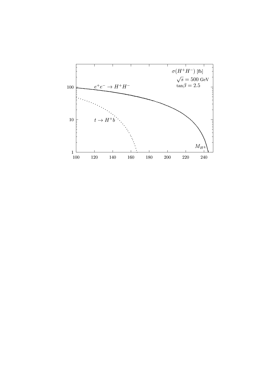
Figure 16: Production cross sections for the charged Higgs boson in $e^{+}e^{-}$ collisions as a function of the $H^{\pm}$ mass for a c.m. energy $\sqrt{s}=500$ GeV and for the decay $t\rightarrow H^{+}b,\mbox{tan}\beta=2.5$.

The program is written in FORTRAN and has been tested on several machines. All the necessary subroutines [e.g. for integration] are included. The program is lengthy but rather fast [especially if some options, e.g. ISHELH, are switched off]. The results for the many production cross sections in femtobarns are written into several output files [with headers indicating the processes and giving the inputs]:

$${\rm zps.out}: M_{H^{0}}\ ,\ \sigma(H^{0}Z)\ ,\ \sigma(H^{0}\nu\bar{\nu})\ ,\ \sigma(H^{0}e^{+}e^{-})$$

$${\rm zpt.out}: M_{H^{0}}\ ,\ \sigma(WW\rightarrow H^{0}H^{0})\ ,\ \sigma(ZZ\rightarrow H^{0}H^{0})\ ,\ \sigma(H^{0}H^{0}Z)\ ,\ \sigma(t\bar{t}H^{0})$$

$${\rm zpl.out}: M_{A}\ ,\ M_{h}\ ,\ \sigma(hZ)\ ,\ \sigma(h\nu\bar{\nu})\ ,\ \sigma(he^{+}e^{-})\ ,\ \sigma(hA)$$

$${\rm zph.out}: M_{A}\ ,\ M_{H}\ ,\ \sigma(HZ)\ ,\ \sigma(H\nu\bar{\nu})\ ,\ \sigma(He^{+}e^{-})\ ,\ \sigma(HA)$$

$${\rm zpc.out}: M_{A}\ ,\ M_{H^{\pm}}\ ,\ \sigma(e^{+}e^{-}\rightarrow H^{+}H^{-})\ ,\ \sigma(t\bar{t}\rightarrow H^{+}H^{-})$$

  MA             Mh          hZ       hnunu       he+e-      hA
 50.0000      48.0416      22.09      52.00      5.483      32.98
 100.000      79.7747      37.30      72.05      7.658      17.48
 150.000      97.2542      52.94      91.32      9.741      4.564
 200.000      103.804      57.82      95.56      10.21      1.019
 250.000      106.497      58.98      95.78      10.23     0.2473

Tab. 4a: The output file zpl.out for the input file in Tab. 3.

 50.0000      131.191      37.36      46.92      5.032      13.66
 100.000      143.719      22.15      25.60      2.750      20.38
 150.000      173.380      6.506      6.176     0.6653      20.11
 200.000      215.038      1.625      1.164     0.1257      8.726
 250.000      261.096     0.4601     0.2384     0.2575E-01  0.000

Tab. 4b: The output file zph.out for the input file in Tab. 3.

  MA           MH+       ee->H+H-     tt->H+H-
 50.0000      92.1414      98.79      53.73
 100.000      126.452      78.94      24.77
 150.000      168.790      49.36      0.5294
 200.000      214.453      16.70      0.000
 250.000      261.706      0.000      0.000

Tab. 4c: The output file zpc.out for the input file in Tab. 3.

In a future version of the code, we will implement the remaining higher order processes [discussed previously] of the SM and for the $h$ boson in the MSSM, and include the $\gamma\gamma$ option of the collider. We also plan to make an interface with the programs SUSPECT [section 3.2] and HDECAY [which calculates the total decay widths in a more precise way]. Beamstralung will also be incorporated by making and interface with the program CIRCEE. The Higgs boson production at hadron machines will be included in the next–to–leading version of the code.

4.3.2 Higgs boson production in association with light stops

As previously discussed [section 3.1 and above], if the off–diagonal entries in the $\tilde{t}$ mass matrix is large, the eigenstate $\tilde{t}_{1}$ can be rather light and at the same time its couplings to the Higgs bosons strongly enhanced. The $h\tilde{t}_{1}\tilde{t}_{1}$ coupling would be then the potentially largest coupling in the electroweak sector of the MSSM, and its measurement would allow to pin down some of the soft–SUSY breaking parameters of the MSSM Lagrangian, in particular the trilinear coupling $A_{t}$. This coupling can be measured in the process $pp\rightarrow\tilde{t}_{1}\tilde{t}_{1}h$ at the LHC [see section 4.1.3]. However, this coupling can be best measured in the associated production process $e^{+}e^{-}\rightarrow\tilde{t}_{1}\tilde{t}_{1}h$ [12]. This is first due to the fact that the cleaner environment of high–energy electron-positron colliders allows for a more efficient search of this complicated final state, ans also because of the very high–luminosity expected at such machines [for instance for the DESY–machine TESLA: $\int{\cal L}\sim 500$ fb^-1 in a year], which compensates for the fact that the process is of higher order in perturbation theory and has a small cross section in priciple.

At future linear $e^{+}e^{-}$ colliders, the final state $\tilde{t}_{1}\tilde{t}_{1}h$ may be generated in three ways:

a) Two–body production and decay:

If the center of mass energy of the $e^{+}e^{-}$ collider is high enough, one first produces a mixed pairs of top squarks, $e^{+}e^{-}\rightarrow\tilde{t}_{1}\tilde{t}_{2}$, through the exchange of a virtual $Z$–boson, and then makes the heaviest top squark decay into the lightest stop and the Higgs boson, $\tilde{t}_{2}\rightarrow\tilde{t}_{1}h$, if the splitting between the two stops is larger than the $h$ boson mass. In principle, if phase–space allowed, the cross section for the two–body production process times the branching ratio for the two–body decay should be large enough for the final state to be copiously produced.

However, the $Z\tilde{t}_{1}\tilde{t}_{2}$ coupling is proportional to $\sin 2\theta_{t}$ while the $h\tilde{t}_{1}\tilde{t}_{2}$ coupling is proportional to $\cos 2\theta_{t}$; since in a large part of the MSSM parameter space [as discussed in section 4.1.3] $\sin 2\theta_{t}$ is either small [no–mixing case] or close to one [maximal mixing case], the cross section times branching bratio, which is then proportional to $\sin 4\theta_{q}$, is always rather small. [In addition, the decay width $\tilde{t}_{2}\rightarrow h\tilde{t}_{1}$ is in general much smaller than the $\tilde{t}_{2}$ decay widths into chargino and neutralinos]. Nevertheless, there are limited regions of the MSSM parameter space where the rate for this process is visible for the high luminosities $\int{\cal L}\sim 500$ fb^-1 expected at the linear colliders.

b) Production in the continuum in e⁺e^- collisions:

There are three types of Feynman diagrams leading to $\tilde{t}_{1}\tilde{t}_{1}h$ finale states in $e^{+}e^{-}$ collisions: Higgs boson emission for the $\tilde{t}_{1}$ lines which proceeds through s–channel photon and $Z$–boson exchange, Higgs boson emission from the $\tilde{t}_{2}$ lines which proceeds through $Z$–boson exchange, and Higgs boson emission from a virtual $Z$ boson which then splits into $\tilde{t}_{1}\tilde{t}_{1}$ pairs. When the $g_{h\tilde{t}_{1}\tilde{t}_{1}}$ coupling is large, the two last types of Feynman diagrams give negligible contributions since the virtuality of $\tilde{t}_{2}$ is large and the $Z\tilde{t}_{1}\tilde{t}_{1}$ coupling not enhanced. The Dalitz plot density of the process [in terms of the scaled energies of the two stops] can be then written in a very simple form.

As an illustration, the total cross section for the process $e^{+}e^{-}\rightarrow h\tilde{t}_{1}\tilde{t}_{1}$ is shown in Fig. 17 as a function of the lightest stop mass for a c.m. energy $\sqrt{s}=500$ GeV, for the values $\tilde{A}_{t}=1.5$ TeV and $\mbox{tan}\beta=3,30$. One can see that below masses of the order of $m_{\tilde{t}_{1}}\sim 160$ GeV, the cross section is larger than 1 fb, leading to $\sim 500$ events with the expected luminosity quoted above. The final state topologies have been discussed in section 4.1.3; however, here the main decay mode of the $h$ boson, $h\rightarrow b\bar{b}$, can be used [this calls for good micro–vertex detectors]. With the relatively large sample of events, this final state should be experimentally possible to be detected even after efficiencies have been included. Higher c.m. energies would allow to probe larger stop masses. The cross section for this process has also been calculated in Ref. [89] using the package SUSY–GRACE; it has been shown that combined with the $e^{+}e^{-}\rightarrow\tilde{t}_{1}\tilde{t}_{1}$ production cross section, the SUSY parameters of the stop sector can be determined.

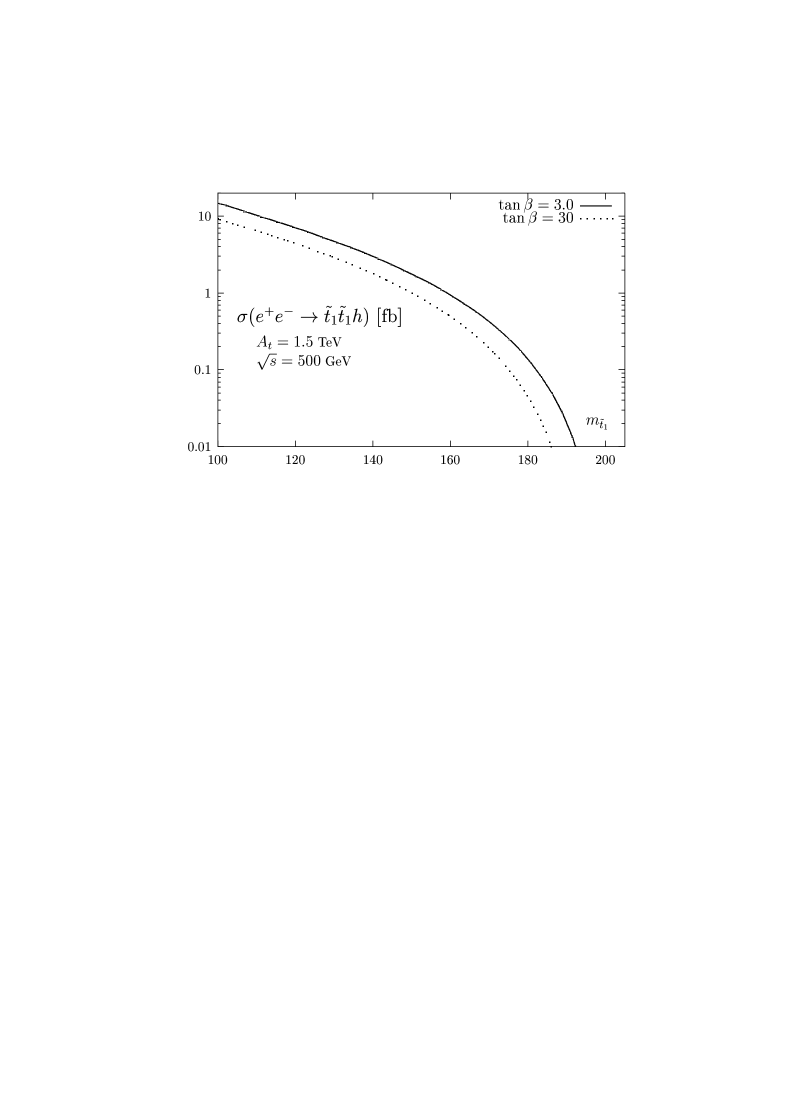
Figure 17: The cross section for the process $e^{+}e^{-}\rightarrow h\tilde{t}_{1}\tilde{t}_{1}$ as a function of the lightest stop mass for a c.m. energy $\sqrt{s}=500$ GeV and for the values $\tilde{A}_{t}=1.5$ TeV and $\mbox{tan}\beta=3,30$.

c) Production in the continuum in $\gamma\gamma$ collisions:

In the $\gamma\gamma$ option of future high–energy $e^{+}e^{-}$ linear colliders, with the high energy photons coming from Compton back–scattering of laser beams, the final state $\tilde{t}_{1}\tilde{t}_{1}h$ can be generated by emitting the $h$ boson from the stop lines in the process $\gamma\gamma\rightarrow\tilde{t}_{1}\tilde{t}_{1}$. In Ref. [12], the cross section for this reaction has been calculated, and the analytical expression has been found to be slightly more complicated than the one obtained in the $e^{+}e^{-}$ mode.

However, because the c.m. energy of the $\gamma\gamma$ collider is expected to be only $\sim 80\%$ of the one of the original $e^{+}e^{-}$ machine, the process is less phase–space favored. In addition, the collected luminosity is expected to be somewhat smaller than the one of the $e^{+}e^{-}$ mode, leading to a smaller number of events. Nevertheless, the cross section for the $\tilde{t}_{1}\tilde{t}_{1}h$ final state is of the same order as in the $e^{+}e^{-}$ mode for c.m. energies not too close to the kinematical threshold, and the process might be useful to obtain complementary information since it does not involve the $Z$–boson and $\tilde{t}_{2}$ exchanges.

5. SUSY Particle Production and Decays

5.1. Virtual SUSY effects

Virtual effects of supersymmetry, for example through gauge boson self–energy or gauge boson–fermion–fermion vertex corrections, are known to be invisibly small at the $Z$ resonance unless the masses of the SUSY particles are very small, a situation which is by now excluded or unlikely [55]. It has been noticed [90] that this property does not apply for energies beyond the $Z$ peak due to the raise of box diagrams. At LEP1 energies, the box contributions are strongly suppressed as they do not benefit of the enhancement due to the $Z$ resonance. Beyond this energy, one can expect them to become relatively important. This is what happens in the standard electroweak case with the box diagrams due to $WW$ formation and neutrino exchanges, where their effect reaches the percent level in the cross section for $e^{+}e^{-}\to\mu^{+}\mu^{-}$ at $\sqrt{s}\sim 200$ GeV. A second source of local box enhancement is the threshold effect appearing around $s=(m_{i}+m_{j})^{2}$ where $m_{i}$ and $m_{j}$ are the masses of the particles formed in the intermediate state. In the aforementioned $WW$ box diagrams the contribution peaks at 1.2$\%$ around 161 GeV.

With this standard situation in mind, one can look at the SUSY box contributions due to charginos or neutralinos and sleptons for the production of light fermion pairs [13]. The case of $\chi^{0}_{i}$–$\chi^{0}_{j}$–slepton boxes is particularly favored for several reasons: the usual gaugino–fermion–sfermion couplings have full electroweak strength, and the box contribution is not mixed with other significant virtual corrections [self–energy, vertex corrections] involving neutralino pairs since the gaugino components are decoupled from gauge bosons and their higgsino components are decoupled from light fermions, so it should be easier to single out this contribution. In order to disentangle such contributions from other effects affecting the $Z$ boson tail, it is convenient to use the so–called “$Z$–peak subtraction method” [91] which consists in using as inputs the measured $Z$–parameters [mass, partial widths and asymmetries] and to describe the additional contributions to the observables beyond the $Z$–peak in terms of four functions constructed with a subtraction at $s=M^{2}_{Z}$. In this way, one eliminates all known or unknown effects contributing at the $Z$–peak and to the $Z$ boson tail, which do not have a strong $s$–dependence.

A first numerical exploration, assuming that neutralinos as well as the left– and right–handed sleptons are degenerate, has been made [13]. This choice allows to greatly simplify the computation as in this case one can use sum rules for reducing the lengthy expressions in the box amplitude. For simplicity neutralinos were also taken as pure wino and bino states. Results are shown in Fig. 18 for the $e^{+}e^{-}\to\mu^{+}\mu^{-}$ cross section and forward–backward asymmetry, for a common neutralino mass $m_{\chi^{0}}=100$ GeV and a slepton mass $m_{\tilde{e}}=60$ GeV. As expected, a peak associated to the threshold effect appears at $s=4m_{\chi^{0}}^{2}$, which reaches the level of 1.5% in the cross section and 0.7% in the FB asymmetry. The half–width is of about 15 GeV.

The level reached by these contributions is very encouraging since such a precision for the cross section is certainly possible at LEP2 [92]; in the case of the FB asymmetry the observability is more difficult. Increasing the $\tilde{e}$ mass to 110 GeV, the peak cross section however decreases roughly by a factor of two. In the case of chargino boxes, assuming again $m_{\chi^{+}}=100$ GeV and $m_{\tilde{\nu}}=60$ GeV, one obtains a similar effect on the cross section and on the forward–backward asymmetry [in this case, the sign is opposite]. However, in contrast to the neutralino case, there now exist other important chargino effects in gauge boson self–energies and vertex corrections; cancellations among these various contributions occur and depend on the masses and couplings of the SUSY particles.

These results are promising since from a general point of view they suggest that virtual SUSY particle effects may be observable at LEP2. A complete study for both neutralino and chargino contributions at LEP2, including all possible effects within the MSSM and varying the parameters in their allowed domain, is under way.

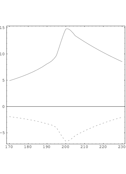
Figure 18: Neutralino box effects on muon pair production at LEP2 energies. Relative effect in permille on the cross section (solid) and on the forward-backward asymmetry (dashed) as a function of the c.m. energy.

5.2 Correlated production and decays in $e^{+}e^{-}\rightarrow\chi_{1}^{+}\chi_{1}^{-}$

Once charginos will have been discovered, the experimental analysis of their properties, production and decay mechanisms, should reveal the basic structure of the underlying low–energy supersymmetric theory. This needs precise experimental measurement, which are more likely to be performed in the clean environment of $e^{+}e^{-}$ colliders. In the case of the chargino sector, three parameters are needed to describe it completely: $\tan\beta,\mu$ and $M_{2}$. One needs therefore several experimental observables to pin down these parameters.

In $e^{+}e^{-}$ collisions, charginos are produced either in diagonal or in mixed pairs [93]. Since the second chargino is generally expected to be significantly heavier than the first state, at LEP2 and potentially even in the first phase of $e^{+}e^{-}$ linear colliders, the lightest chargino $\tilde{\chi}_{1}^{\pm}$ may be, for some time, the only state that can be studied in detail. It is therefore wiser to focus on the diagonal pair production of the lightest chargino $e^{+}e^{-}\rightarrow\chi^{+}_{1}\chi^{-}_{1}$. The production process is generated by $s$–channel $\gamma$ and $Z$ exchanges, and $t$–channel $\tilde{\nu}$ exchange. It will depend on the two angles $\phi_{L}$ and $\phi_{R}$ [more precisely on $\cos 2\phi_{L}$ and $\cos 2\phi_{R}$] which define the chargino–chargino–$Z$ and the electron–sneutrino–chargino vertices, the chargino mass $m_{\chi_{1}^{+}}$ and the sneutrino mass $m_{\tilde{\nu}}$. Thus at least four measurements are needed to determine these parameters.

However, the situation is complicated by the decays of the charginos. Indeed, the charginos will decay into the lightest neutralino and light fermion pairs [93] and since the two neutralinos are stable and escape undetected, it is not possible to make a complete reconstruction of the events; in particular, one cannot measure the $\chi^{\pm}_{1}$ production angle. Furthermore, the chargino decays occur through $W$ boson and sfermion [and also a marginal contribution from charged Higgs boson] exchanges, and the knowledge of the sfermion masses and couplings is in principle also required.

Recently it has been shown [14] that even in this situation the underlying SUSY parameters can be extracted from the mass $m_{\chi^{\pm}_{1}}$, the total production cross section, and the measurement of the polarization with which the charginos are produced. The $\chi^{\pm}$ polarization vectors and $\chi$–$\chi$ spin–spin correlation tensors can be determined from the decay distributions of the charginos. Beam polarization is helpful but not necessarily required. No detailed information on the decay dynamics, nor on the structure of the neutralino, is needed to carry out the spin analysis. There are already several analyses dealing with polarized chargino production [see Ref. [94] or the contribution of Katsanevas et al. [95] for instance]; Ref. [14] however attempts to explore analytically the event characteristics as will be summarized below.

Since the $\chi^{\pm}_{1}$ lifetime is very small, only the correlated production and decay can be observed experimentally

where $n$ and $\bar{n}$ are the spin 4–vectors and $p,\bar{p}$ the momenta of the charginos. In covariant language the final state distributions are found by combining the polarized cross section

$${\rm d}\sigma=\langle{\rm d}\sigma\rangle\frac{1}{4}\left[1-{\cal P}^{\mu}n_{\mu}-\bar{\cal P}^{\mu}\bar{n}_{\mu}+{\cal Q}^{\mu\nu}n_{\mu}\bar{n}_{\nu}\right]$$ (5.1)

with the polarized distributions for the decays into a neutralinos and light fermion pairs

$${\rm d}\Gamma=\langle{\rm d}\Gamma\rangle\left[1-{\cal P}^{{}^{\prime}\mu}n_{\mu}\right]\ \ \ \ {\rm d}\bar{\Gamma}=\langle{\rm d}\bar{\Gamma}\rangle\left[1-\bar{\cal P}^{{}^{\prime}\mu}\bar{n}_{\mu}\right]$$ (5.2)

Inserting the completeness relations $\sum n_{\mu}n_{\nu}=-g_{\mu\nu}+p_{\mu}p_{\nu}/m^{2}_{\tilde{\chi}^{-}_{1}}=\eta_{\mu\nu}$ etc, the overall event topology can then be calculated from the formula

$${\rm d}\sigma_{\rm final} = \langle{\rm d}\sigma\rangle\langle{\rm d}\Gamma\rangle\langle{\rm d}\bar{\Gamma}\rangle\frac{1}{4}\bigg{[}1+\eta_{\mu\alpha}{\cal P}^{\mu}{\cal P}^{{}^{\prime}\alpha}+\bar{\eta}_{\nu\beta}\bar{\cal P}^{\nu}\bar{\cal P}^{{}^{\prime}\beta}+\eta_{\mu\alpha}\bar{\eta}_{\nu\beta}{\cal Q}^{\mu\nu}{\cal P}^{{}^{\prime}\alpha}\bar{\cal P}^{{}^{\prime}\beta}\bigg{]}$$ (5.3)

In these expressions ${\cal P}({\cal P}^{\prime})$ and $\overline{\cal P}(\overline{\cal P}^{\prime})$ are the polarization vectors of the produced (decaying) $\chi^{-},\chi^{+}$ states, while ${\cal Q}_{\mu\nu}$ is the chargino spin–spin correlation matrix.

In the case of CP–invariance [the CP non–invariant case has been discussed in Ref. [96]], the overall topology is determined by seven independent functions: the unpolarized cross section $\sigma_{\rm unpol}$, the two components of the polarization vector of one of the charginos, and four correlation functions. Except for $\sigma_{\rm unpol}$, these observables will depend on the final state, and hence on the decays of the charginos into neutralinos and fermion pairs. However, it was shown [14] that it is possible to construct two observables, denoted by ${\cal P}^{2}/{\cal Q}$ and ${\cal P}^{2}/{\cal Y}$, which do not depend on the chargino decays and hence, reflect unambiguously the properties of the chargino system, being not affected by the neutralinos. The energy dependence of the ratios ${\cal P}^{2}/{\cal Q}$ and ${\cal P}^{2}/{\cal Y}$ is shown in Fig. 19 for $\tan\beta=2$ and for the $(M_{2},\mu)$ parameters chosen as: gaugino region ($81,-215)$ GeV, higgsino region $(215,-810)$ GeV and mixed region $(92,-93)$ GeV, which lead to a chargino mass $m_{\chi^{\pm}_{1}}\sim 95$ GeV. The two ratios are sensitive to the couplings at sufficiently large c.m. energies.

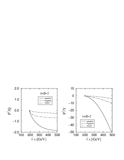
Figure 19: The energy dependence of the ratios ${\cal P}^{2}/{\cal Q}$ and ${\cal P}^{2}/{\cal Y}$ for $\tan\beta=2$.

Therefore, in addition to the chargino mass $m_{{\chi}^{\pm}_{1}}$ which can be measured very precisely near the threshold where the production cross section $\sigma(e^{+}e^{-}\rightarrow{\chi}^{+}_{1}{\chi}^{-}_{1})$ rises sharply with the velocity, and the $\tilde{\nu}$ mass which can be determined with the energy variation of the cross section [in case where the determination of $m_{\tilde{\nu}}$ is poor, longitudinal beam polarization might be helpful to eliminate the $t$–channel $\tilde{\nu}$ exchange], we have two observables which allow to determine the two mixing angles $\cos 2\phi_{L}$ and $\cos 2\phi_{R}$. A representative example of determining these two parameters is shown in Fig. 20 at a c.m. energy $\sqrt{s}=500$ GeV for the “measured” values: $m_{{\chi}^{\pm}_{1}}=95\ {\rm GeV},\sigma(e^{+}e^{-}\rightarrow{\chi}^{+}_{1}{\chi}^{-}_{1})=0.38\ {\rm pb},{\cal P}^{2}/{\cal Q}=-0.25,{\cal P}^{2}/{\cal Y}=-5.0$. The three contour lines meet at a single point $(\cos 2\phi_{L},\cos 2\phi_{R})=(-0.60,-0.49)$ for $m_{\tilde{\nu}}=250$ GeV.

Figure 20: Contours for the “measured values” of the total cross section, ${\cal P}^{2}/{\cal Q}$ and ${\cal P}^{2}/{\cal Y}$ for $m_{{\chi}^{\pm}_{1}}=95$ GeV [$m_{\tilde{\nu}}=250$ GeV].

Once $\cos 2\phi_{L},\cos 2\phi_{R}$ and $m_{{\chi}^{\pm}_{1}}$ are known, the SUSY parameters $\tan\beta,M_{2},\mu$ can be then determined with at most a two–fold discrete ambiguity. Introducing the two triangular quantities $p=\cot(\phi_{R}-\phi_{L})$ and $q=\cot(\phi_{R}+\phi_{L})$ and solving the set

$$p^{2}+q^{2}=2\frac{s_{L}^{2}+s_{R}^{2}}{(c_{L}-c_{R})^{2}}\ ,\ p^{2}-q^{2}=\frac{4s_{L}s_{R}}{(c_{L}-c_{R})^{2}}\ ,\ pq=\frac{c_{L}+c_{R}}{c_{L}-c_{R}}$$ (5.4)

with $c_{L,R}=\cos 2\phi_{L,R}$ and $s_{L,R}=\sin 2\phi_{L,R}$, the solutions $(p,q)$ in point (1) and point (2) of Fig. 21 are found for $\sin 2\phi_{L}\sin 2\phi_{R}>0$ or $<0$, and a second set is found by reversing the signs of the solutions pairwise. From this, one obtains for $\tan\beta$:

$$\cos 2\phi_{R}>\cos 2\phi_{L}\ \ :\ \ \tan\beta=\frac{p^{2}-q^{2}\pm 2\sqrt{\chi^{2}(p^{2}+q^{2}+2-\chi^{2})}}{(\sqrt{1+p^{2}}-\sqrt{1+q^{2}})^{2}-2\chi^{2}}\;\Rightarrow\;\tan\beta\geq 1$$ (5.5)

where $\chi^{2}=m^{2}_{{\chi}^{\pm}_{1}}/M^{2}_{W}$. If the denominator is positive, there are either up to two solutions for $\tan\beta>+1$ in point (1) and none in point (2), or at most one in point (1) and at most one in point (2). The possible solutions can be counted in an analogous way if the denominator is negative; the rôles of point (1) and point (2) are just interchanged. The same counting is also valid in the second case $\cos 2\phi_{R}<\cos 2\phi_{L}:\tan\beta\rightarrow 1/\tan\beta$. Thus, only a two–fold ambiguity is inferred from all solutions in point (1) and point (2).

The gaugino and higgsino mass parameters are given in terms of $p,q$ by:

$$\left(\begin{array}[]{c}M_{2}\\ \mu\end{array}\right)=\frac{M_{W}}{\sqrt{2}}\bigg{[}(p\pm q)\sin\beta-(p\mp q)\cos\beta\bigg{]}$$ (5.8)

The parameters $M_{2}$, $\mu$ are uniquely fixed if $\tan\beta$ is chosen properly in point (1) and/or point (2). Since $\tan\beta$ is invariant under pairwise reflection of the signs in $(p,q)$, the definition $M_{2}>0$ can be exploited to remove this additional ambiguity. Returning to the “experimental values” of mass, cross section and spin correlations introduced above, the following parameters are extracted for point (2) $[\tan\beta;M_{2},\mu]=[1.0;53~{}{\rm GeV},-52~{}{\rm GeV}]$ or $[1.4;240~{}{\rm GeV},137~{}{\rm GeV}]$. Point (1) gives negative values for $\tan\beta$ so that the solution derived from the “experimental values” is unique in this case.

Thus, the fundamental SUSY parameters $\tan\beta;M_{2},\mu$ can be derived from the observables $m_{{\chi}^{\pm}_{1}}$ and $\cos 2\phi_{R}$, $\cos 2\phi_{L}$ up to at most a two–fold ambiguity, by considering the production of the lightest chargino pair and using the partial information on the chargino polarizations. Moreover, from the energy distribution of the final particles in the decay of the chargino, the mass of the lightest neutralino can also be measured; this allows to determine the parameter $M_{1}$ so that also the neutralino mass matrix can be reconstructed in a model–independent way.

Figure 21: Determination of $(p,q)$ from $p^{2}+q^{2}$, $pq$ and $p^{2}-q^{2}$ for $pq>0$.

5.3 Chargino/neutralino production at hadron colliders

5.3.1 Theoretical cross sections

Because they are strongly interacting, squarks and gluinos are the most copiously produced SUSY particles at hadron colliders, and the processes $pp\rightarrow\tilde{g}\tilde{g},\tilde{q}\tilde{q},\tilde{q}\tilde{g}$ have been extensively discussed in the literature; for a review see Ref. [22]. However, the charginos and neutralinos might be the lightest SUSY particles, and would be the first to be kinematically accessible. In addition, even if the existence of supersymmetry would be established by the detection of squarks and gluinos at the LHC, the direct production of charginos and neutralinos would allow various tests of the model, and is therefore very interesting to investigate.

Except for squark and gluino production, the next potentially largest cross section for SUSY particles at the LHC is the one for the production of the lightest chargino and the next–to–lightest neutralino:

$$pp\ \rightarrow\ qq\ \rightarrow\ \chi_{2}^{0}\ \chi_{1}^{\pm}$$ (5.9)

Although it is an electroweak process, the production rates are large enough to allow for a copious number of events at the LHC, even at a low luminosity ${\cal L}=10$ fb^-1. The process is of the Drell–Yan type, and proceeds via $s$–channel $W$ boson exchange and $t$–channel squark exchange. In this section we revisit the tree–level calculation for the partonic cross section of this process, and this for two reasons: $(i)$ this is a good warming–up exercise using the semi–automatic program FeynMSSM that we are developing for SUSY computations, which we will describe briefly later on, and which we plan to use, in the future, to calculate the one–loop QCD and electroweak radiative corrections to this process; $(ii)$ compare our independent calculation with two existing and disagreeing results in the literature [97, 98] to settle the issue. By doing so we also took the opportunity to compare our notations [mainly based on Ref. [45] and subsequent papers] with the notations of the previous references [which, of course, are also distinct from each other…]. For more details the reader is referred to Ref. [15].

The differential cross–section for the subprocess has been given in both Refs. [97] and [98]. However the only place where the result of Ref. [97] can be found in an analytical form is in the program ISAJET. When this expression is extracted from the code and compared with the one given in Ref. [98], one finds a discrepancy. The formula from ISAJET reads

$$d\sigma/dt = 1/(16\pi s^{2})[{\cal A}_{s}(U+T)/{\cal D}_{s}+{\cal A}_{s}^{\prime\prime}(U-T)/{\cal D}_{s}$$ (5.10)

$$+{\cal A}_{s}^{\prime}\ (m_{\chi_{1}^{+}}m_{\chi_{2}^{0}})s/{\cal D}_{s}+{\cal A}_{u}\ U/{\cal D}_{u}^{2}+{\cal A}_{t}T/{{\cal D}_{t}^{\prime}}^{2}$$

$$+{\cal A}_{st}\ (s-M_{W}^{2})T/({\cal D}_{s}{\cal D}_{t}^{\prime})$$

$$+{\cal A}_{st}^{\prime}\ m_{\chi_{1}^{+}}\ m_{\chi_{2}^{0}}s(s-M^{2}_{W})/({\cal D}_{s}{\cal D}_{t}^{\prime})+{\cal A}_{su}\ U(s-M^{2}_{W})/({\cal D}_{s}{\cal D}_{u})$$

$$+{\cal A}_{su}^{\prime}\ m_{\chi_{1}^{+}}\ m_{\chi_{2}^{0}}s(s-M^{2}_{W})/({\cal D}_{s}{\cal D}_{u})+{\cal A}_{tu}\ s\ m_{\chi_{1}^{+}}\ m_{\chi_{2}^{0}}/({\cal D}_{u}{\cal D}_{t}^{\prime})]$$

where

$$U=(m^{2}_{\chi_{1}^{+}}-u)(m^{2}_{\chi_{2}^{0}}-u)\ ,\ T=(m^{2}_{\chi_{1}^{+}}-t)(m^{2}_{\chi_{2}^{0}}-t)$$ (5.11)

$m_{\chi_{1}^{+}}$ and $m_{\chi_{2}^{0}}$ are respectively the chargino and neutralino masses and $u,\ t$ and $s$ the Mandelstam variables. ${\cal D}_{s}$ and ${\cal D}_{u}$ are given by

$${\cal D}_{s} = (s-M^{2}_{W})^{2}+M^{2}_{W}\Gamma^{2}_{W}\ ,\ {\cal D}_{u}=(u-m^{2}_{{\tilde{u}_{L}}})\ ,$$ (5.12)

$${\cal D}_{u}^{\prime} = (u-m^{2}_{\tilde{d}_{L}})\ ,\ {\cal D}_{t}^{\prime}=(t-m^{2}_{\tilde{d}_{L}}).$$ (5.13)

where $m_{\tilde{d}_{L}},m_{{\tilde{u}_{L}}}$ are the left–handed down and up squark masses respectively. The factors ${\cal A}^{(^{\prime},^{\prime\prime})}$ encapsulate the information on the chargino–neutralino couplings to $W$ bosons and sfermions. Eq. (5.10) agrees with the corresponding one in Ref. [98] apart from the term ${\cal A}_{s}^{\prime\prime}$ which is missing in the latter. We repeated the calculation in a completely independent way and found full agreement with eq. (5.10) thus re–ensuring the validity of the expression used by ISAJET.

This calculation has been performed with the program FeynMSSM, which is based on the packages FeynArts [which generates the full set of diagrams automatically] and FeynCalc [which calculates the amplitudes, and reduces them to the standard forms] developed [99] for a semi–automatic calculation of amplitudes in the Standard Model. FeynMSSM, incorporates the MSSM Feynman rules [following the notations of Ref. [45]] and thus generates the amplitudes for any SUSY process in principle. The program is running under Mathematica2.0, and has been checked for processes with up to three particles in the final state, as well as loop diagrams [up to two loops] which is in fact the main purpose of the program. When FeynMSSM will be fully operational, the hope is that it would be very efficient and useful when dealing with higher–order processes, either multi–loop or multi–final state, in the MSSM.

5.3.2 Searches at the LHC

Let us now turn to the discussion of this process at the LHC. To suppress the huge QCD backgrounds, one needs to look at signatures with isolated leptons in the final state, and the many leptons there are the smaller will be the backgrounds. The one–lepton channel suffers from the large number of singly produced $W$ bosons, while the two–lepton channel suffers from single $Z$ boson and $WW$ pair production. One should then look at the signal with three leptons plus missing energy. The leptons of the signals will come from the decays of the chargino into a $W$ boson and the LSP, and the decay of the next–to–lightest neutralino into a $Z$ boson and the LSP. The branching ratios are sizeable in a large area of the MSSM parameter space, despite of the small branching ratios of the gauge boson [especially the $Z$ boson] decays into charged leptons. The main background reactions are due to $WZ$ and $ZZ$ production, as well as the semi–leptonic decays of heavy quarks and the $Zb\bar{b}$ background. There are also backgrounds from the production of other SUSY particles, and in particular squark and gluino production [which then decay, among other final states, into the studied neutralino and chargino via cascades] and associated chargino/neutralino production with a squark or a gluino; there are also backgrounds from the pair production of charginos and neutralinos.

The signal can be distinguished from the background events, mainly due to the lower hadronic activity and not from the amount of missing energy; applying a set of standard [ATLAS] cuts [59], one can obtain a $5\sigma$ signal at the low luminosity LHC for gluino masses smaller than $\sim 500$ GeV; see Ref. [100] for details. Furthermore, the mass difference between the produced neutralino and the LSP, $m_{\chi_{2}^{0}}-m_{\chi_{1}^{0}}$, can be measured precisely from the invariant mass distribution the lepton pair coming from $Z$ decays.

In this section, we propose to use the charge asymmetry

$$A=(N_{+}-N_{-})/(N_{+}+N_{-})$$ (5.14)

where $N_{+}(N_{-})$ is the number of positively (negatively) charged leptons, as a new observable in LHC analyses in processes where charged particle final states are produced [16]. What is exploited is the fact that, contrary to LEP and the Tevatron, the LHC is an asymmetric machine as far as the electric charge is concerned. Indeed, at the LHC we expect to produce more $W^{+}$ than $W^{-}$ bosons, since the proton contains as valence quarks two $u$ and one $d$ quarks and the process $u\bar{d}\rightarrow W^{+}$ is more favored than $\bar{u}d\rightarrow W^{-}$.

It has been noticed in Ref. [16] that the charge asymmetry increases linearly with increasing mass of the formed final state. It can be therefore used for indirect measurement of particle masses, based only on the structure functions. This has been checked with PYTHIA 6.114 for the events $W\rightarrow e\nu_{e}$ or $\mu\nu_{\mu}$ using the structure functions CTEQ4 [75], and varying artificially the $W$ boson mass. This exercise has been repeated for the process $pp\rightarrow WZ\rightarrow 2\;{\rm jets}+e\nu_{e}$ and $2\;{\rm jets}+\mu\nu_{\mu}$, which exhibits the same behavior. To check that this effect was not due to the particular choice of the structure functions, we used a different set of parton densities and the result was the same, except of course for the different slope of the charge asymmetry as a function of the mass.

These results are illustrated in Fig. 22, where the charge asymmetry in percent is plotted against the mass of the final $W$ or $WZ$–system at the LHC with $\sqrt{s}=14$ TeV, using the CTEQ4M parton densities. The two dark points at $M\simeq 80$ and $171$ GeV correspond to the asymmetries of the $W$ and $WZ$ systems, which are respectively 19% and 21%. The brighter circles and crosses correspond respectively to the asymmetries of the $W$ and $WZ$ systems when the effective mass is varied [in the latter case, the ratio $M_{W}/M_{Z}$ is kept constant]. One notices that these asymmetries are quite substantial, $\sim 15$ to $35$%, and can be therefore experimentally measurable.

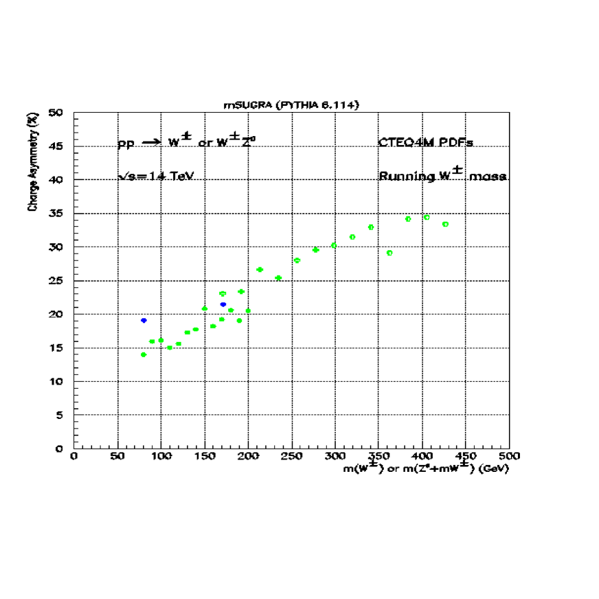
Figure 22: The charge asymmetry [in %] as a function of the mass of the final $W$ or $WZ$–system at the LHC with $\sqrt{s}=14$ TeV, using the CTEQ4M parton densities.

In Ref. [16], it has been therefore proposed to apply this method to the process $pp\rightarrow\chi_{2}^{0}\chi_{1}^{\pm}\rightarrow 3l^{\pm}$+ missing energy. Let us first recall that the production amplitude is dominated by the $s$–channel $W$ boson exchange for heavy enough squarks. In this diagram, the $u\bar{d}W^{+}$ vertex depends only on the proton structure function, and is completely independent of the final SUSY state. However, this vertex decides of the $W$ boson charge, and thus on the global charge of the chargino and the trilepton event. One can measure the charge asymmetry of the set of events which passes the cuts needed to extract the signal, and determine the sum of the masses $m_{\chi_{2}^{0}}+m_{\chi_{1}^{+}}$. In Fig. 23, this mass was varied by scanning the MSSM parameter space, and the obtained asymmetry is shown. As can be seen, the charge asymmetry is always proportional to the mass of the final system.

To confirm the usefulness of this method to measure the $\chi$ masses, a detailed Monte-Carlo simulation including the signals and backgrounds which pass the selection cuts is required. Although not very precise [there is a systematic bias from the used structure functions, and there is still a small dependence on the SUSY parameters due to the small interference between the $s$–channel $W$ exchange and the $t$–channel squark exchange amplitudes], the results are encouraging and the method deserves further investigations.

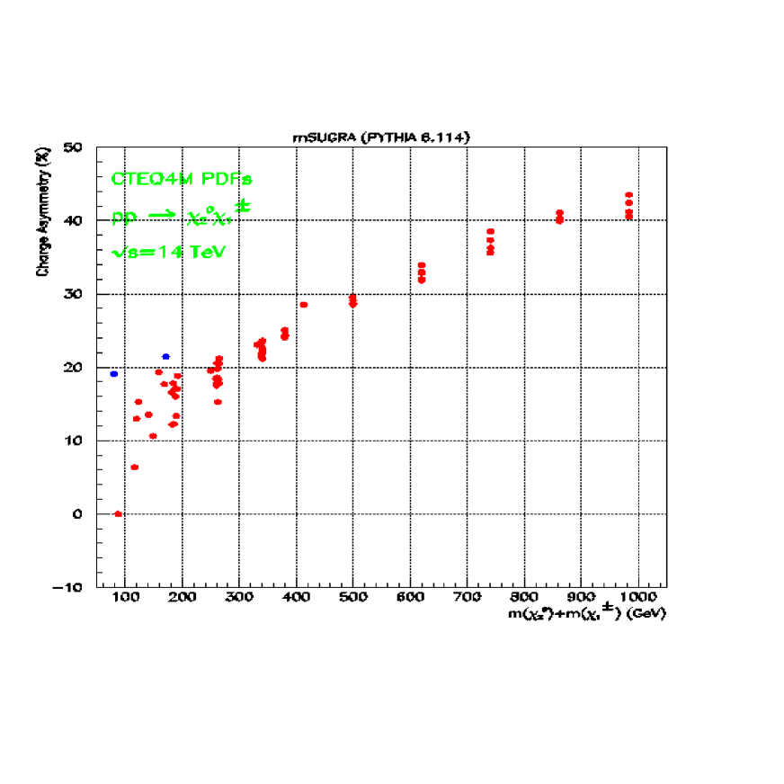
Figure 23: The charge asymmetry [in %] a function of $m_{\chi_{2}^{0}}+m_{\chi_{1}^{+}}$ at the LHC with $\sqrt{s}=14$ TeV, using the CTEQ4M parton densities.

5.4 Two– and three–body sfermion decays

The dominant decay modes of scalar fermions are the two–body decays into their partner fermions plus neutralinos or charginos:

$$\tilde{f}_{i}\rightarrow f\chi_{j}^{0}\ \ ,\ \ \tilde{f}_{i}\rightarrow f^{\prime}\chi_{j}^{\pm}$$ (5.15)

In general at least the decays into the lightest neutralino [which is the lightest SUSY particle] and chargino is kinematically available. In the case of squarks, if their masses are larger than the sum of the partner quark and the gluino masses, the decay

$$\tilde{q}\rightarrow q\tilde{g}\ \ {\rm if}\ \ m_{\tilde{q}}>m_{q}+m_{\tilde{g}}$$ (5.16)

largely dominates since it is a strongly interacting process. These decays are well–known; see for instance Ref. [22] for a discussion.

In the case of the third generation sfermions, and in particular for stops, the mixing can be so important that a large splitting between superpartners is generated; see section 2.4. This opens the possibility of decays of sfermions into lighter sfermions and gauge bosons or Higgs bosons:

$$\tilde{f}_{i} \rightarrow \tilde{f}^{\prime}_{j}+W^{\pm}\ ,\ \tilde{f}^{\prime}_{j}+H^{\pm}$$ (5.17)

$$\rightarrow \tilde{f}_{j}+Z\ ,\ \tilde{f}_{j}+h,A,H$$

These decays, including the mixing between sfermions have been discussed recently; see Ref. [101] for instance.

Finally, the mass of the lightest stop could be smaller than the sum of the top and LSP masses, and smaller than the lightest chargino mass. In this case the only allowed decay mode will be into a charm quark and the lightest neutralino through loops [102]

$$\tilde{t}_{1}\rightarrow c\chi_{1}^{0}$$ (5.18)

There are many situations, however, where these two–body decays of sfermions are suppressed or kinematically inaccessible. This happens for instance for the lightest stop and sbottom squarks in the case of large sfermion mixing, and for the scalar partners of the light quarks in models where the gaugino mass unification constraint is relaxed, and in gauge mediated SUSY breaking models. In this case, various three–body modes might become relevant. A list of three–body decays of sfermions which might be important includes:

$(i)$ Decays of the stops into a $b$–quark, a neutralino and a $W$ or $H^{+}$ boson:

$$\tilde{t}_{1,2}\rightarrow t^{*},\tilde{b}^{*},\chi^{+*}\rightarrow b\;\chi_{1}^{0}\;W^{+}\ \ {\rm or}\ \ b\;\chi_{1}^{0}\;H^{+}$$ (5.19)

The decay $\tilde{t}\rightarrow b\chi_{1}^{0}W^{+}$ is especially important in the case of the lightest stop, when it is lighter than $m_{b}+m_{\chi^{+}_{1}}$ and $m_{t}+m_{\chi_{1}^{0}}$. In this case, the lightest stop $\tilde{t}_{1}$ will decay into a charm quark plus the lightest neutralino, eq. (5.18). Because it is loop mediated, this decay has a partial decay width that is suppressed by four powers of the electroweak coupling and by the CKM angle $V_{cb}$, compared to the usual two–body decay widths. In this case, the three–body decay into $b\chi^{0}W$ with a virtual exchange of a top quark, a sbottom and a chargino might become competitive. In fact, the decay is also suppressed by two powers of the electroweak coupling as well as by the virtuality of the exchanged particles; however, there are some kinematical regions where this mode dominates over the $\tilde{t}_{1}\rightarrow c\chi_{1}^{0}$ decay channel. This decay mode has been also discussed in Ref. [103], where however only the matrix elements in terms of the four momenta of the particles involved have been given.

The decay $\tilde{t}\rightarrow b\chi_{1}^{0}H^{+}$ is similar to the previous one with the $W$ boson replaced by the charged Higgs boson $H^{+}$. In the MSSM the charged Higgs boson is always heavier than the $W$ and this in principle disfavors this process kinematically compared to decay into $Wb\chi_{1}^{0}$. However, the couplings of the $H^{+}$ boson to the third generation quarks and squarks can be strongly enhanced, leading to a possible compensation. For relatively small masses of the $H^{\pm}$ boson, the decay branching ratio of this channel can be sizeable.

$(ii)$ Decays of the heavier stop into the lighter stop or sbottom and a fermion pair:

$$\tilde{t}_{2}\rightarrow Z^{*},h^{*},A^{*}\rightarrow\tilde{t}_{1}f\bar{f}\ ,\ \tilde{t}_{2}\rightarrow W^{*},H^{+*}\rightarrow\tilde{b}f\bar{f}^{\prime}$$ (5.20)

This decay occurs when the states $\tilde{t}_{1}$ or $\tilde{b}$ are rather light and there is a splitting between the two stops and/or between $\tilde{t}_{2}$ and the sbottoms, while the mass differences $m_{\tilde{t}_{2}}-m_{\tilde{t}_{1}}$ or $m_{\tilde{t}_{2}}-m_{\tilde{b}}$ are still smaller than $M_{Z},M_{h},M_{A}$ or $M_{W},M_{H^{\pm}}$, respectively. When $\tilde{t}_{2}$ is lighter than $m_{b}+m_{\chi^{\pm}_{1}}$ and $m_{t}+m_{\chi^{0}}$, the two–body decays [except for the loop decay $\tilde{t}\rightarrow c\chi_{1}^{0}$] are forbidden, and these three–body modes become relevant. For high values of $\tan\beta$ the corresponding decays of the heavier sbottoms [i.e. the stops replaced by the sbottoms in the decays above] might also be of some relevance.

$(iii$) Decays of squarks into quarks and a stop or a sbottom via gluino exchange:

$$\tilde{q}\rightarrow\tilde{g}^{*}\rightarrow q\;t\;\tilde{t}\ \ {\rm or}\ \ q\;b\;\tilde{b}$$ (5.21)

The decay $\tilde{q}\rightarrow qb\tilde{b}$ of a scalar partner of a light quark occurs when gluinos are heavier than the squark [but not too much because the large virtuality of the exchanged gluino will strongly suppress the decay] and when there is a strong mixing in the sbottom sector which makes that the lightest sbottom is lighter than all other squarks. One also needs that the lightest chargino and neutralinos are rather heavy and/or of almost higgsino type to suppress their couplings to the squarks. However, in models with the unification of the gaugino masses at the GUT scale, the gluino and chargino/neutralino masses are related and for not too heavy gluinos [not to suppress the decay width by the $\tilde{g}^{*}$ virtuality] the decays into the other chargino and/or neutralinos are still allowed kinematically and would dominate since these particles would be then of the gaugino type. However, relaxing the assumption of gaugino mass universality, one can find a large area of the parameter space where the mode eq. (5.21) can be sizeable.

For small values of $\tan\beta$, it is the mixing in the $\tilde{t}$ sector which can be strong and $\tilde{t}_{1}$ possibly lighter than the other squarks; a similar situation as previously occurs then for the decay $\tilde{q}\rightarrow qt\tilde{t}$ despite of the kinematical complication of having a top quark in the decay product which requires larger decaying squark masses than in the previous case.

$(iv$) Decays of squarks into quarks and a slepton–lepton pair via chargino and/or neutralino exchange:

$$\tilde{q}\rightarrow\chi^{0*}\ ,\chi^{\pm*}\rightarrow q\tilde{l}l$$ (5.22)

This decay occurs when sleptons are lighter than squarks and the squark decays into neutralinos and charginos are kinematically shut or suppressed by the small squark–quark–higgsino couplings. This happens for instance in gauge mediated supersymmetry breaking models where, first the gravitino which couples only weakly to squarks is the LSP and in addition there is a hierarchy which makes the squarks heavier than sleptons. The next–to–lightest particles could then be the sleptons [and in particular the stau’s because of the mixing for large values of $\tan\beta$]. If squarks have masses smaller than the chargino or neutralino masses so that the two–body decays $\tilde{q}\rightarrow\chi^{0}q,\chi^{\pm}q^{\prime}$ are kinematically closed, the modes eqs. (5.22) become the dominant ones.

However, even in the “phenomenological MSSM” discussed before, these decays are possibly important if the lightest neutralinos and charginos are pure higgsinos [thus suppressing the squark–quark–ino couplings and the two–body decays into quarks+inos] and the other charginos and neutralinos are not much heavier than the sleptons [not to be hurt by the virtually of these states]; the relaxation of the gaugino mass unification assumption will help in enlarging the MSSM parameter range where this situation occurs. The three–body decay modes of first/second generation sleptons into third generation sleptons+leptons have also been discussed in Ref. [104] in the context of gauge mediated breaking models.

All these decays are discussed in detail in Ref. [17]. The Dalitz plot densities for the partial widths d$\Gamma$/(d$x_{1}$d$x_{2}$), where $x_{1}$ and $x_{2}$ are the scaled energies of two final particles, are given including the full dependence on the final fermion/sfermion masses and on the couplings [sfermion mixing is included for instance]. The two remaining integrations are then performed numerically to obtain the partial decay widths and the branching ratios. In the cases where there is only one massive particle in the final state [such as in case ($iv)$, $(iii)$ for sbottoms and in case $(ii)$ for both stops and sbottoms] the integration can be done analytically and is given.

A detailed discussion of the relative magnitude of the decay modes $(i)$–$(iv)$ is given in Ref. [17]. In addition, the fortran code calculating the partial widths and branching ratios is available. It is based on the subroutines SFERMION, GAUGINO and SUSYCP [which calculate the masses and couplings of sfermions, charginos/neutralinos and Higgs bosons respectively] included in the program SUSPECT discussed in section 3.2. Therefore, an interface with SUSPECT is easily possible and will be done in a near future.

5.5 Stop and sbottom searches at LEP200

As discussed previously, squarks of the third generation, namely the stops and the sbottoms, have a special place in the SUSY spectra due to the particular Yukawa couplings of their partners, the top and bottom quarks; stops and sbottoms could even have masses accessible at LEP200. In this section we discuss the searches of these squarks at LEP200 [18], focusing on the scenarii where R–parity is conserved and in both the unconstrained MSSM and the mSUGRA models. The notations and conventions are those introduced in Section 3.

5.5.1 Squark production at LEP200

At LEP200, squarks of the same mass are pair–produced through $\gamma/Z$ s–channel exchange. One notes that the squark–squark–Z boson coupling can vanish for the special value of the mixing angle: $\theta_{q}=A_{q}\cos(\sqrt{e_{\tilde{q}}s_{W}^{2}/I_{3}^{q}})$, which corresponds to 0.98 rad for the stop and 1.17 rad for the sbottom. At the Born level, the production cross section is given by [105]:

$$\sigma^{\rm Born}={{\pi\alpha^{2}}\over{s}}\beta^{3}\left[e_{\tilde{q}}^{2}+\left({{(v_{e}^{2}+a_{e}^{2})v_{\tilde{q}}^{2}}\over{16s_{W}^{4}c_{W}^{4}}}s^{2}-{{e_{\tilde{q}}v_{e}v_{\tilde{q}}}\over{2s_{W}^{2}c_{W}^{2}}}s(s-M_{Z}^{2})\right){1\over{(s-M_{Z}^{2})^{2}+\Gamma_{Z}^{2}M_{Z}^{2}}}\right]$$ (5.23)

with $v_{e}=2s^{2}_{W}-1/2$, $a_{e}=-1/2$ and $v_{\tilde{q}}=2(I_{3}^{q}\cos^{2}\theta_{q}-Q_{\tilde{q}}\sin^{2}\theta_{W})$; $\beta$ is the squark velocity. This cross section is minimal for:

$$\cos^{2}\theta_{\rm min}={e_{f}s_{W}\over I_{3}^{q}}\left[1+\left(1-{{M_{Z}^{2}}\over{s}}c_{W}^{2}\right){{L_{e}+R_{e}}\over{L_{e}^{2}+R_{e}^{2}}}\right]$$ (5.24)

with $L_{e}=s_{W}^{2}-1/2$ and $R_{e}=s_{W}^{2}$. The mixing angle values are equal, up to a level of 5 $\%$, to those corresponding to a vanishing squark–squark–Z boson coupling.

The QCD corrections are factorizable and one obtains for pure gluon exchange and emission in the final state [106, 107]:

$$\sigma^{\rm QCD}=\sigma^{\rm Born}\left[1+{4\over 3}{{\alpha_{s}}\over{\pi}}f(\beta)\right]\ \ ;\ \ f(\beta)\simeq{{\pi^{2}}\over{2\beta}}-{{1+\beta}\over{2}}\left({{\pi^{2}}\over 2}-3\right)$$ (5.25)

[the expression of $f(\beta)$ is given in the Schwinger approximation which reproduces the complete formula at the 1.5 $\%$ level]. In the high energy limit $\beta\rightarrow 1$, $f(\beta)\;\rightarrow\;3$ leading to a correction four times higher than the one corresponding to quark production in the same limit.

The electromagnetic corrections can be taken into account by convoluting the cross section with [106]:

$$L_{ee}(x)=\left[\beta_{em}(1-x)^{\beta_{em}-1}(1+{3\over 4}\beta_{em})-{1\over 2}\beta_{em}(1+x)\right]\left[1+\alpha_{em}\left({\pi\over 3}-{1\over{2\pi}}\right)\right]$$ (5.26)

where $\beta_{em}=2\alpha_{em}/\pi\left({\rm Log}(s/m_{e}^{2})-1\right)$ and $\alpha_{em}$ the QED coupling constant defined at zero–momentum transfer. One obtains then the total cross section:

$$\sigma^{\rm tot}(e^{+}e^{-}\rightarrow\tilde{q}\tilde{q}^{*})=\int_{0}^{1}L_{ee}(x)\sigma^{\rm QCD}(xs)dx$$ (5.27)

The various cross sections: $\sigma^{\rm Born}$, $\sigma^{\rm QCD}$, $\sigma^{\rm QED}$ and the total cross section $\sigma^{\rm tot}$ including all corrections are shown in Fig. 24 at a c.m. energy $\sqrt{s}=172$ GeV in the case of the lightest stop and sbottom squarks with masses of 80 GeV and as function of the squark mixing angles. One can see that the QCD corrections, which are always positive, increase when $m_{\tilde{q}}\rightarrow\sqrt{s}/2$, reaching 60$\%$ for a 80 GeV stop mass. They are constant and equal to 15$\%$ far from the production threshold. QED corrections are negative near the kinematical threshold and positive when otherwise. Close to threshold, the QED corrections tend to compensate the QCD corrections and the result is a total cross section equal at the level of 5$\%$ for $m_{\tilde{q}_{1}}$=80 GeV to that of the Born approximation.

Figure 24: Stop and sbottom production cross sections at $\sqrt{s}$=172 GeV as a function of the mixing angles and for a squark mass of 80 GeV.

5.5.2 Squark decays

In this section we discuss the decays of the stop and sbottom squarks in the framework of the uMSSM and mSUGRA. Let us first concentrate on the case of the lightest stop. According to the discussion in the previous section on sfermion decays, there are only a few decay modes relevant for stop masses that are kinematically accessible at LEP200, i.e. $m_{\tilde{t}_{1}}\raisebox{-3.69899pt}{~{}\shortstack{$<$ \\ [-0.07cm] $\sim$}}~{}100$ GeV:

– The loop induced flavor changing two body decay mode into a charm quark and the lightest neutralino, $\tilde{t}_{1}\rightarrow c\chi_{1}^{0}$, always occurs since the lightest neutralino is the LSP. The decay width is given by [102]:

$$\Gamma(\tilde{t}_{1}\rightarrow c\chi_{1}^{0})={{\alpha}\over{4s_{W}^{2}}}|\epsilon|^{2}m_{\tilde{t}_{1}}b_{i1}\left[1-{{m^{2}_{\chi^{0}_{i}}}\over{m^{2}_{\tilde{t}_{1}}}}\right]^{2}$$ (5.28)

where $b_{i1}$ depend on the neutralino parameters $\mu,M_{1},M_{2},{\rm tan}\beta$. The $\epsilon$ parameter takes into account the various possible loop contributions and is estimated [102] to be $\epsilon\sim(1-4)\times 10^{-4}$. This small value has the consequence that the stop decay time is far longer than the strong-interaction time scale, $\tau_{QCD}\sim 10^{-23}$ s. If this channel dominates, the stop hadronises first before decaying. The corresponding decay into charm plus a gluino is ruled out for stop masses accessible at LEP200, due the experimental bound on the gluino mass from Tevatron [55].

– The three–body decays $\tilde{t}_{1}\rightarrow bl^{+}\tilde{\nu}$ and $\tilde{t}_{1}\rightarrow b\tilde{l}^{+}\nu$ through the exchange of an off–shell chargino are allowed if $m_{\tilde{t}_{1}}>m_{\tilde{\nu}}+m_{b}$ or $m_{\tilde{t}_{1}}>m_{\tilde{l}}+m_{b}$. The corresponding widths can be found in [102]. The first of these decays is more favored by kinematics since the experimental limit [55] on the sneutrino mass, $m_{\tilde{\nu}}\raisebox{-3.69899pt}{~{}\shortstack{$>$ \\ [-0.07cm] $\sim$}}~{}37$ GeV is weaker than the one for charged sleptons, $m_{\tilde{l}}\raisebox{-3.69899pt}{~{}\shortstack{$>$ \\ [-0.07cm] $\sim$}}~{}$ 65–85 GeV depending on the flavor. The other possible three–body final states are: $\tilde{t}_{1}\rightarrow\;bW^{+}\chi_{1}^{0}$ and $\tilde{t}_{1}\rightarrow\;bH^{+}\chi_{1}^{0}$ through exchanges of sbottom, chargino or top quark. Nonetheless, in the MSSM, the $H^{+}$ mass is larger than the $W$ boson mass, and the experimental bound on the LSP [55] tends to close this channel.

– The decay into a bottom and the lightest chargino $\tilde{t}_{1}\rightarrow b\chi_{1}^{+}$ if charginos are lighter than stops. However, since the experimental limit on the lightest chargino mass is rather strong $m_{\chi_{1}^{+}}\raisebox{-3.69899pt}{~{}\shortstack{$>$ \\ [-0.07cm] $\sim$}}~{}90$ GeV [55], this decay occurs only for stop masses close to 100 GeV. However, when it occurs, this decay mode largely dominates since it occurs at the tree–level and is a two–body decay.

Thus the most likely decay modes of stops at LEP200 are the $\tilde{t}_{1}\rightarrow c\chi_{1}^{0}$ and $\tilde{t}_{1}\rightarrow bl\tilde{\nu}$. To illustrate the relative magnitude of these two channels we make the following assumptions: $(i$) The lightest neutralino $\chi_{1}^{0}$ is the LSP, ($ii$) the lightest stop is lighter than the lightest chargino, and $(iii)$ the lightest stop is heavier than the sleptons. Furthermore, we shall use the following experimental bounds on the sparticle masses from direct and indirect searches: a) $m_{\tilde{\nu}}>$ 37 GeV, b) $m_{\tilde{l}}>$ 85, 65 et 67 GeV for selectrons, smuons and staus respectively and c) $m_{\tilde{g}}>$ 150 GeV [55]. We vary the parameters $M_{2}$ and $\mu$ in the range [0,1000] GeV and $[-1000,1000]$ GeV, respectively .

Fig. 25 shows the accessible region in the plane $(\mu,M_{2})$ for which we have $m_{\chi^{+}_{1}}>$ 80 GeV and $m_{\chi_{1}^{0}}<m_{\tilde{t}_{1}}$= 80 GeV. The stop mixing angle has been fixed to $\theta_{t}$=0 and $\theta_{t}=\pi/2$. The stop partial widths for the two decay modes $\tilde{t}_{1}\rightarrow c\chi_{1}^{0}$ and $\tilde{t}_{1}\rightarrow b\tau\tilde{\nu}$ have been calculated for two sneutrino masses: $m_{\tilde{\nu}}$=42 GeV and 70 GeV. Contours in the $[M_{2},\mu$] plane for the branching ratios of the decay mode $\tilde{t}_{1}\;\rightarrow\;c\chi_{1}^{0}$ are shown. One can see that this decay mode is largely dominating, with a branching ratio larger than 99%, except for small sneutrino masses [which makes the decay mode $\tilde{t}_{1}\rightarrow b\tau\tilde{\nu}$ more phase–space favored] and small stop mixing angle [which favors one of the higgsino or wino components of the charginos]. Indeed, for $\theta_{t}=0$, the $\tilde{t}b\chi_{1}^{+}$ coupling depends both on the wino and higgsino components. Nonetheless, if the chargino is higgsino–like, the $\chi_{1}^{+}l\tilde{\nu}$ coupling is proportional to the tau Yukawa coupling which is in that case very small [remember that we are dealing with small ${\rm tan}\beta$ values]; this means that for $\theta_{t}$=0, the decay $\tilde{t}_{1}\rightarrow bl\tilde{\nu}$ has non negligible values only for a wino–like $\chi_{1}^{+}$ that is for $|\mu|\gg M_{2}$ and this is precisely the region where this decay dominates. On the other hand, for $\theta_{t}=\pi/2$, the coupling stop-bottom-chargino only depends on the higgsino component of $\chi_{1}^{+}$ and the decay $\tilde{t}_{1}\rightarrow\;bl\tilde{\nu}$ is then suppressed because the chargino–lepton–sneutrino coupling is in that case governed by the lepton Yukawa coupling and is negligible.

Figure 25: Contours for the branching ratio $\tilde{t}_{1}\rightarrow c\chi_{1}^{0}$ in the $(\mu,M_{2})$ plane for: ${\rm tan}\beta$=2, $m_{\tilde{t}_{1}}$=80 GeV, $m_{\chi_{1}^{+}}>$ 80 GeV, $m_{\tilde{\nu}}$=42 or 70 GeV, $\theta_{t}$=0 or $\pi/2$.

The analysis of the stop branching ratio is simpler in mSUGRA due to the reduced number of free parameters. Let us compare below the two stop decays $\tilde{t}_{1}\rightarrow\;c\chi_{1}^{0}$ and $\tilde{t}_{1}\rightarrow\;bl\tilde{\nu}$ in the framework of mSUGRA for the following range of parameters: $\alpha_{U}=1/24.3$, $2\leq\tan\beta\leq 8$, $-2.9\leq A_{0}\leq 2.9$ [in TeV], sign($\mu)=\pm$, $0\leq m_{0}\leq 1000$ and $0\leq m_{1/2}\leq 1000$. The regions in the $(m_{0},m_{1/2})$ plane for which the following conditions on the sparticles masses are fulfilled are shown on Fig. 26: $m_{\chi_{1}^{0}}<m_{\tilde{t}_{1}}\leq 80$ GeV (25a), $m_{\chi_{1}^{+}}>80$ GeV (25b) and $m_{\chi_{1}^{0}}<m_{\tilde{\nu}}<m_{\tilde{t}_{1}}\leq 80$ GeV (25c).

The intersection of the domains in Figs. 26a and 26b gives the accessible space for which the decay $\tilde{t}_{1}\rightarrow\;c\chi_{1}^{0}$ is possible with a chargino heavier than the scalar top. One observes that the condition $m_{\chi_{1}^{+}}>$ 80 GeV strongly reduces the possible space; this is due to the universality condition in the gaugino sector which prevents a large mass difference between $\chi_{1}^{0}$ and $\chi_{1}^{+}$. The intersection between the domains in Figs. 26b and 26c is negligible, which implies that the decay $\tilde{t}_{1}\rightarrow\;bl\tilde{\nu}$ is highly improbable if $m_{\chi_{1}^{+}}>$ 80 GeV. If the electroweak symmetry breaking conditions are imposed, the parameter space in the $(m_{0},m_{1/2})$ plane in which this decay can occur is strongly reduced as it is observed in Fig. 26. In conclusion, the decay $\tilde{t}_{1}\;\rightarrow\;c\chi_{1}^{0}$ has a branching ratio near unity in the constrained MSSM; however the corresponding accessible space in the plane $(m_{0},m_{1/2})$ is small, especially if a proper EWSB is required.

Figure 26: Accessible domain for the decay $\tilde{t}_{1}\rightarrow c\chi_{1}^{0}$ in the $(m_{0},m_{1/2})$ plane for the sets of parameters discussed above, and with the requirements: $m_{\chi_{1}^{0}}<m_{\tilde{t}_{1}}$ and $m_{\tilde{t}_{1}}\leq$ 80GeV for a), $m_{\tilde{t}_{1}}\leq$80 GeV and $m_{\chi_{1}^{+}}>$80 GeV for b) and $m_{\chi_{1}^{0}}\leq m_{\tilde{\nu}}\leq m_{\tilde{t}_{1}}$ with $m_{\tilde{t}_{1}}\leq$ 80 GeV for c). The points correspond to cases for which no correct EWSB is required and the bullets to accessible domains with a correct EWSB.

Finally, let us briefly discuss sbottom decays. The only two accessible decay modes from sbottoms which can be produced at LEP200, are $\tilde{b}_{1}\rightarrow b\chi_{1,2}^{0}$ [the decay $\tilde{b}_{1}\rightarrow b\tilde{g}$ is forbidden by Tevatron results]. The relative magnitudes of these two decays depend on the sbottom mixing angle $\theta_{b}$ and on $\mu,M_{2}$ and $\tan\beta$ parameters [we assume here the GUT relation between $M_{1}$ and $M_{2}$]. More precisely, if $M_{2}\gg|\mu|$, $\chi_{1}^{0}$ and $\chi_{2}^{0}$ are higgsino–like and the couplings $\tilde{b}_{1}b\chi^{0}$ do not depend on $\theta_{b}$ and are similar; the decay $\tilde{b}_{1}\rightarrow b\chi_{1}^{0}$ then dominates over the decay $\tilde{b}_{1}\rightarrow b\chi_{2}^{0}$. If $|\mu|\gg M_{2}$ then $\chi_{1}^{0}$ is photino–like and $\chi_{2}^{0}$ is zino–like; the coupling $\tilde{b}_{1}b\tilde{Z}$ is minimal for $\theta_{b}=\pi/2$ and in this case $\tilde{b}_{1}\rightarrow b\tilde{\chi}_{1}^{0}$ dominates over $\tilde{b}_{1}\rightarrow b\chi_{2}^{0}$. On the other hand, the coupling $\tilde{b}_{1}b\tilde{Z}$ is maximal for $\theta_{b}=0$ and is larger than the $\tilde{b}_{1}b\tilde{\gamma}$ coupling, leading to a domination of $\tilde{b}_{1}\rightarrow b\tilde{\chi}_{2}^{0}$ over $\tilde{b}_{1}\rightarrow b\chi_{1}^{0}$. The fact that the sbottom hadronises or not, which is a question of experimental interest when searching for sbottom squarks which are mass–degenerate with neutralinos, also depends on $\theta_{b}$ and $\mu,M_{2},\tan\beta$ but is complicated by the lack of knowledge of the precise QCD time scale. Studies concerning this subject can be found in [18].

6. Experimental bounds on SUSY Particle Masses

6.1. Introduction

A wide range of searches for supersymmetric particles are performed at present colliders and no deviation with respect to the Standard Model predictions was observed yet, unfortunately. Therefore new limits on the masses of these particles, assuming different models, are set by the various experiments. In this section we focus on the experimental results obtained both at LEP and the Tevatron, interpreted in the constrained MSSM or mSUGRA framework [but for LEP2, without the constraint of correct radiative electroweak symmetry breaking and without assuming any mass unification for Higgs bosons with the other scalar particles] assuming that the LSP is the lightest neutralino $\chi^{0}_{1}$ and that R–parity is conserved. In this model, as discussed in section 2, all SUSY particle masses, their couplings and their production cross sections and decay widths are predicted in terms of only five free independent parameters: $m_{1/2},m_{0},\mu,{\rm tan}\beta$ $m_{A}$ and $A$; the renormalization group equations are used to determine the parameters at low energies. Instead of $m_{1/2}$, the LEP experiments usually derive their results as a function of the parameter $M_{2}$, the SUSY breaking mass term associated with the SU(2)_L gauge group ($m_{1/2}\approx M_{2}/0.81$). At the Tevatron, the previous assumptions are made in the interpretation of the results, with the additional constraint of the radiative electroweak symmetry breaking. In this case, $|\mu|$ is no more a free parameter and is determined when $m_{0}$, tan$\beta$, $m_{1/2}$ and the $Z$ boson mass $M_{Z}$ are fixed; the sign of $\mu$ remains free; see section 2.

The searches for supersymmetric particles at LEP2 concern sleptons, stops, sbottoms, charginos and neutralinos as detailed in [108]. These various SUSY particles decay to SM particles and two LSPs; therefore, SUSY signatures consist of some combination of jets or/and leptons and missing energy since the LSP escapes detection. The signal topology and the background conditions are in practice affected by the SUSY particle and the LSP mass difference ($\Delta M=m_{\rm SUSY}-m_{\chi^{0}_{1}})$ which controls the visible energy. In the low $\Delta M(=5-10$ GeV) range, the expected topologies for the signals are characterized by a low multiplicity and a low visible energy and the background is dominated by two–photon interactions. For large $\Delta M(=50-60$ GeV) values, the signal signatures are very similar to those of $W$–pair production. Since all the background sources are due to well calculable processes with reasonable production cross sections compared to the signal, most of the decay channels are studied at LEP2.

Another important key domain concerns the searches for the MSSM Higgs bosons. Presently, only the lighter neutral Higgs bosons $h$ and $A$ can be discovered at LEP2 [109], since the CP–even Higgs boson $H$ and the charged Higgs bosons $H^{\pm}$ are expected to be too heavy. However searches for charged Higgs bosons are also performed at LEP2 in the framework of a non–SUSY two–Higgs doublet model.

After collecting $\sim 150~{}{\rm pb}^{-1}$ at LEP1 ($\rm 1989\rightarrow 1995$), each experiment (ALEPH, DELPHI, L3, OPAL) has accumulated data at LEP2: $\sim 5.5~{}{\rm pb}^{-1}$ at $\sqrt{s}=133$ GeV (1995), $\sim 10~{}{\rm pb}^{-1}$ at $\sqrt{s}=161$ GeV (1996), $\sim 10~{}{\rm pb}^{-1}$ at $\sqrt{s}=172$ GeV (1996) and $\sim 55~{}{\rm pb}^{-1}$ at $\sqrt{s}=183$ GeV (1997). This year, an amount of $150~{}{\rm pb}^{-1}$ at $\sqrt{s}=189$ GeV (October 1998) is already recorded by each experiment, but the results including all the statistics for 1998 are not yet available; a fraction of the overall integrated luminosity is only used corresponding to the statistics collected just before the summer conference time ($\rightarrow$ July 1998 : $30-40~{}{\rm pb}^{-1}$).

At the Tevatron the main sources for SUSY are squarks and gluinos, abundantly produced due to the color factors and the strong coupling constant. Squarks or gluinos are produced in pair, and decay directly or via cascades to at least two LSP’s. The classical searches rely on large missing transverse energy $({\rm E}_{\perp}/\hskip 0.28436pt)$ caused by the escaping LSPs. In addition, charginos and neutralinos are searched for via their leptonic decay channels by the two Tevatron experiments CDF and D0. Finally, searches for the MSSM charged Higgs boson are performed at the Tevatron, and bounds on the charged supersymmetric Higgs boson mass have been set by both experiments. Each experiment has collected an integrated luminosity of about 110 pb^-1 at $\sqrt{s}=1.8$ TeV.

Since no evidence for production of supersymmetric particles has been found, experimental limits on their production cross sections and masses has been derived. In what follows, we will pay attention to all the decay channels used to extract the limits both at LEP2 and Tevatron. The most recent results have been used, including preliminary results reported at the last summer conference in Vancouver and the last LEPC meeting.

6.2 The scalar particle sector

6.2.1 The Higgs bosons

Due to the expected large mass of the heavier CP even Higgs boson $H$, only searches for the neutral $h$ and $A$ bosons will be reported in what follows. These neutral Higgs bosons can be produced at LEP via two complementary processes:

• The Standard Model–like Higgs–strahlung process, $e^{+}e^{-}\rightarrow hZ$; the cross section for this process is equal to its SM analogue, reduced by a factor $\sin^{2}(\alpha-\beta)$ which means that this process occurs mainly at low tan$\beta$ values.

• The associated pair production process, $e^{+}e^{-}\rightarrow hA$, with a cross section proportional to $\cos^{2}(\beta-\alpha)$; this process is dominant at large tan$\beta$ values.

In the first channel, searches are similar to those performed for the SM Higgs boson. For tan$\beta>$1 the main decay modes of the $h$ and $A$ bosons are into $b\bar{b}$, and to a lesser extent $\tau^{+}\tau^{-}$. Most of the experimental analyses required therefore at least two $b$ quarks in the final states, as detailed in Tab. 5. Clearly, $b$–tagging plays a crucial role in all the Higgs searches at LEP; it allows to reach very high sensitivities by rejecting most of the $WW$ background. Peculiar decays such as $h\rightarrow AA$ or $h\rightarrow\chi_{1}^{0}\chi_{1}^{0}$ have been also considered; the sensitivities achieved in the latter case are better compared to those obtained with the standard decay channels at LEP1 but worse at LEP2. Typical efficiencies and background expectations are listed in Tab. 6, where observation and expectation from SM processes agree very well.

Therefore, limits have been extracted [111]–[116], for two “benchmark” sets of the MSSM parameters where $M_{\rm susy}$, representing the stop mass mean value in Figs. 26, is fixed to 1 TeV and $m_{t}=175$ GeV; $M_{A}$ varies up to 2 TeV and $\mbox{tan}\beta$ from 0.5 to 50, and either minimal or no stop mixing [$A=0$ TeV, $\mu=-0.1$ TeV] or maximal squark mixing [$A=\sqrt{6}$ TeV, $\mu=-0.1$ TeV] is assumed.

$\sqrt{s}$ (GeV)	hA	hZ
91	hA $\rm\rightarrow~{}q\bar{q}\tau^{-}\tau^{+},\tau^{-}\tau^{+}q\bar{q}$	Zh$\rm\rightarrow~{}\nu\bar{\nu}q\bar{q}$
	hA$\rm\rightarrow~{}AAA$	Zh$\rm\rightarrow~{}l^{-}l^{+}q\bar{q}$
	AAA$\rm\rightarrow~{}b\bar{b}b\bar{b}b\bar{b}$	Zh$\rm\rightarrow~{}\tau^{-}\tau^{+}q\bar{q}$
		Zh$\rm\rightarrow~{}q\bar{q}~{}\tau^{-}\tau^{+}$
		Zh$\rm\rightarrow~{}q\bar{q}h(\rightarrow\chi^{0}_{1}~{}\chi^{0}_{1})$
136	hA$\rm\rightarrow~{}b\bar{b}b\bar{b}$
	hA$\rm\rightarrow~{}AAA$
	AAA$\rm\rightarrow~{}b\bar{b}b\bar{b}b\bar{b}$
161,172,183	hA$\rm\rightarrow~{}b\bar{b}b\bar{b}$	Zh$\rm\rightarrow~{}\nu\bar{\nu}(h\rightarrow all)$
	hA$\rm\rightarrow~{}b\bar{b}\tau^{-}\tau^{+},\tau^{-}\tau^{+}~{}b\bar{b}$	Zh$\rm\rightarrow~{}l^{-}l^{+}(h\rightarrow all)$
	AAA$\rm\rightarrow~{}b\bar{b}b\bar{b}b\bar{b}$	Zh$\rm\rightarrow~{}\tau^{-}\tau^{+}(h\rightarrow all)$
		Zh$\rm\rightarrow(h\rightarrow all)~{}\tau^{-}\tau^{+}$
		Zh$\rm\rightarrow~{}q\bar{q}b\bar{b}$
		Zh$\rm\rightarrow~{}q\bar{q}$ or $l^{-}l^{+}h(\rightarrow\chi^{0}_{1}~{}\chi^{0}_{1})$

Table 5: Search channels for the neutral Higgs bosons at LEP.

The limits obtained by each experiments within these assumptions are listed in Tab. 7. The combined limit, obtained as described in Ref. [110] leads to a gain of about 3–4 GeV with respect to the individual experiments. Four methods for the combination are used, they all agrees within a spread of $\pm$ 1.9 GeV; conservatively the lower limit is quoted in Tab. 7 (method C of Ref. [110]), while the higher limits (with method D) are given in Figs. 26. These limits are valid for $\mbox{tan}\beta$ greater than 0.8, irrespectively of the mixing value or of the method used for the combination. For the no mixing scenario, the range of $\mbox{tan}\beta$ between 0.8 and 2.1 is excluded independently of the method. It has to be noticed that the limits have been improved, for each LEP experiment, by almost 4 GeV/c² with the recent data collected at 189 GeV [117], reaching therefore the level of the combined limit at 183 GeV. It has been pointed out recently in Refs. [116],[114],[112], that selected sets of the MSSM parameters lead to less stringent exclusions, either because of an unexpectedly small bremsstrahlung cross section or because of a reduced decay branching ratio into $b\bar{b}$. The analysis of Ref. [112] shows however that the probability of occurrence of such sets is extremely small, typically at the $10^{-3}$ level. The theoretical status of these pathological parameter sets is currently under investigation. Meanwhile, the limits obtained in the benchmark cases can be regarded as sufficiently robust for practical purposes.

Selection	$\epsilon$(%) for hZ	$\rm N_{signal}^{exp}$	$\rm N_{Bkg}^{exp}$	$\rm N^{obs}$
	$\rm M_{h}$=80 GeV$/c^{2}$
$\rm hl^{+}l^{-}$	78.3	1.1	2	3
$\rm h\nu\bar{\nu}$	20.9	0.8	0.16	0
$\rm b\bar{b}q\bar{q}$	23.6	3.6	1.4	1
$\rm b\bar{b}\tau^{+}\tau^{-}$	22.7	0.14	0.17	0
$\rm\tau^{+}\tau^{-}q\bar{q}$	9.8	0.16	0.16	0
Selection	$\epsilon$(%) for hA	$\rm N_{signal}^{exp}$	$\rm N_{Bkg}^{exp}$	$\rm N^{obs}$
	$\rm M_{h}=M_{A}$=75 GeV$/c^{2}$
$\rm b\bar{b}b\bar{b}$	60.5	3.1	2.4	2
$\rm b\bar{b}\tau^{+}\tau^{-}$	28.6	0.27	0.07	0

Table 6: Typical efficiencies and expected/observed number of events for the neutral Higgs bosons searches performed by the ALEPH experiment [111] at $\sqrt{s}$=183 GeV.

	$\rm M_{h,A}$ lower limit ($\rm GeV/c^{2})$
	up to $\sqrt{s}=183$ GeV
	Range of	lower
	Individual Limit	LEP combined
	(ADLO)
h (Obs.)	70.7–74.4	78.8
(Exp.)	67.4–70.3	76.3
A (Obs.)	71.0–76.1	79.1
(Exp.)	68.4–72.0	76.3

Table 7: Individual and LEP combined mass limits for the neutral $h$ and $A$ bosons [110].

At the Tevatron, the most widely studied mechanism for producing neutral Higgs bosons is the associated production of the CP–even $h$ boson with a $W$ or $Z$ boson. In addition, one has to require the gauge boson to decay leptonically; this reduces the observable rate by a factor greater than 75 %. Therefore a collected luminosity of several fb^-1 is needed to reach a sensitivity competitive with those achieved at LEP. Recently, in Ref. [119], it has been made use of the fact that the $Ab\bar{b}$ coupling is proportional to $\tan\beta$, i.e. the cross section production grows as $\tan^{2}\beta$. Analyzing the events from CDF containing $\tau^{-}\tau^{+}+2$ jets in the final state [used to set limits on third generation leptoquarks], the authors derived new bounds in the plane ($M_{A},\mbox{tan}\beta$); in particular if the mass of the CP–odd Higgs boson is just beyond the present limit, the $\mbox{tan}\beta$ region above 80 is excluded.

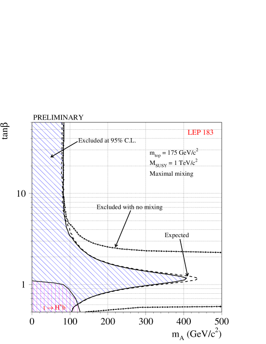
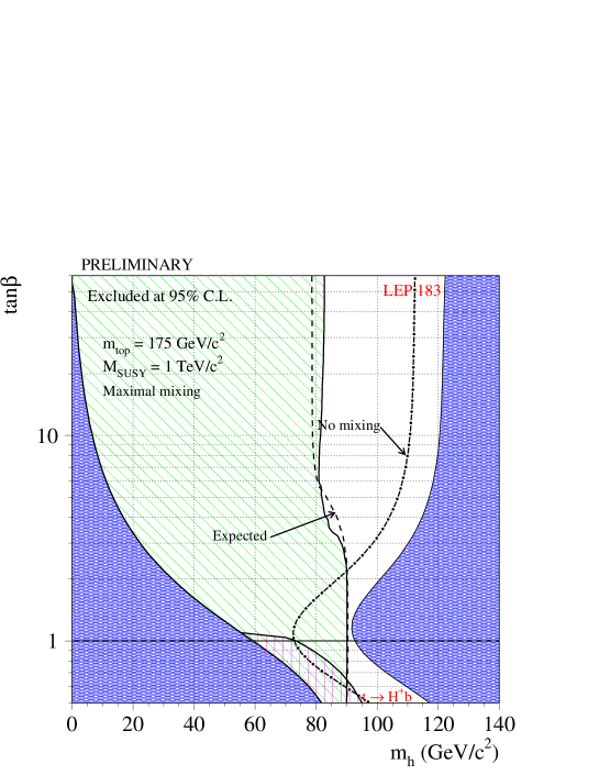
Figure 26: LEP combined exclusion domains (method D) in the plane $\rm(M_{A},\mbox{tan}\beta)$ (top) or $\rm(M_{h},\mbox{tan}\beta)$ (bottom) by the LEP direct searches for $\rm e^{+}e^{-}\rightarrow$ hZ and hA at center-of-mass energies up to 183 GeV assuming either a maximal mixing or no mixing [110] and [118].

Let us now turn to charged Higgs bosons. The $H^{\pm}$ bosons can be produced in $e^{+}e^{-}$ interactions via the process $e^{+}e^{-}\rightarrow\gamma^{*},Z^{*}\rightarrow H^{+}H^{-}$ and are expected to decay mainly into the heaviest lepton kinematically allowed and its associated neutrino, or into the heaviest kinematically allowed quark pair whose decay widths are not Cabibbo suppressed; the relative branching ratios are model dependent. Therefore searches are performed in the three possible decay modes: $e^{+}e^{-}\rightarrow H^{+}H^{-}\rightarrow\tau^{-}\bar{\nu_{\tau}}\tau^{+}\nu_{\tau}$, $\tau^{+}\nu_{\tau}s\bar{c}$ and $c\bar{s}s\bar{c}$. For each experiment [120]– [123] and each decay channel, the number of selected events in the data is consistent, with the number of expected events from SM processes, as can be seen in Tab. 8. Compared to the neutral Higgs boson searches, the sensitivities achieved are lower; this is due to the high $WW$ background contamination.

$\rm M_{H^{\pm}}$=60 $\rm GeV/c^{2}$	$\tau^{+}\bar{\nu}_{\tau}\tau^{+}\nu_{\tau}$	$\tau^{+}\nu_{\tau}s\bar{c}$	$c\bar{s}s\bar{c}$
Efficiency	24 %	42 %	40 %
Expected events	9.2	30.1	99.4
Observed events	6	28	93

Table 8: Typical efficiencies, number of expected and observed events obtained by the L3 experiment in the charged Higgs boson searches at c.m. energy of 183 GeV [122].

	$\rm M_{H^{\pm}}\>$ Lower limit ($\rm GeV/c^{2})$
	up to $\sqrt{s}=183$ GeV
	Range of	Lower
	Individual Limit (ADLO)	LEP combined
H± (Obs.)	56.6–59.0	68.0
(Exp.)	56.0–62.0	69.0

Table 9: Individual and LEP combined mass limits for the charged Higgs bosons.

The 95 % C.L. individual limits on the charged Higgs boson mass is shown as a function of the branching ratio Br($H^{\pm}\rightarrow\tau^{\pm}\nu_{\tau})$ in Fig. 28. Combining all LEP results, a lower limit on the charged Higgs boson mass of 68 GeV is established at the 95 % C.L., assuming just that the sum BR$(H^{+}\rightarrow\tau^{+}\nu_{\tau})$ + Br$(H^{+}\rightarrow c\bar{s})$ is equal to one. It represents a gain of almost 10 GeV with respect to the individual limits, Tab. 9.

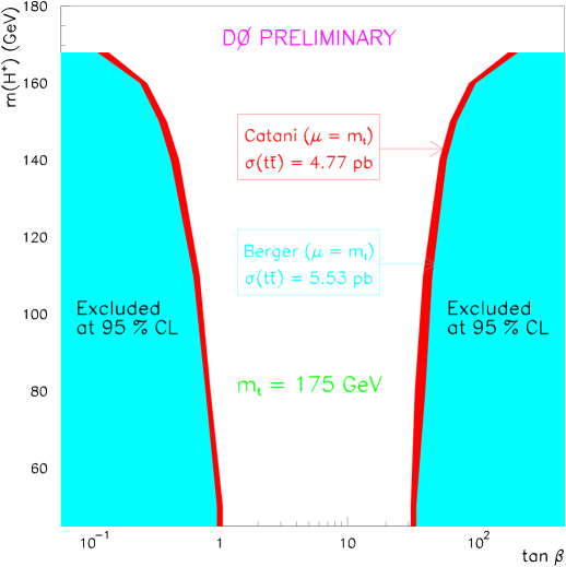
Figure 27: LEP combined exclusion domains in the plane ($M_{H^{\pm}},Br(\rm H^{\pm}\rightarrow\tau\nu_{\tau})$) by the LEP direct searches for $\rm e^{+}e^{-}\rightarrow H^{+}H^{-}$ at center-of-mass energies up to 183 GeV [110].

Figure 28: D0 exclusion domains [125] in the plane ($\tan\beta,M_{H}^{\pm}$) from top decay.

In the MSSM, the charged Higgs bosons are expected to be heavier than the $W$ boson, and can be searched for in the decay products of the top quarks that are produced at the Tevatron. If the charged Higgs boson is light enough, the two possible decay channels for the top are either $t\rightarrow{W^{+}}b$ or $t\rightarrow{H^{+}}b$; as an example for $M_{H^{\pm}}=100$ GeV, the decay $t\rightarrow H^{+}b$ becomes dominant for both large ($\raisebox{-3.69899pt}{~{}\shortstack{$>$ \\ [-0.07cm] $\sim$}}~{}30$) and low ($\raisebox{-3.69899pt}{~{}\shortstack{$<$ \\ [-0.07cm] $\sim$}}~{}1$) $\mbox{tan}\beta$ values. Moreover for low $\mbox{tan}\beta$ values $H^{+}$ decays dominantly into $c\bar{s}$ leading to final states containing six jets without isolated leptons. The measurement of the top branching ratio into $W^{+}b$, tagged with leptonic events, allows to set an upper limit on the branching ratio of the decay $t\rightarrow H^{+}b$, assuming an expected $t\bar{t}$ production cross section not larger than 5.6 pb; CDF [124] and D0 [125] set a limit of about 25 % which can be turned into excluded regions in the ($M_{H^{\pm}},\mbox{tan}\beta$) plane as depicted in Fig. 28. For instance, for $M_{H^{\pm}}=100$ GeV, all $\mbox{tan}\beta$ values below 1.1 and above 40 are excluded by Tevatron searches [118]. These limits may be also turned into excluded region in the plane ($M_{h},\mbox{tan}\beta$) as depicted in bottom Fig. 26 [118] and [110].

6.2.2. Scalar leptons

LEP experiments excluded scalar neutrinos with masses up to 43 GeV, from the comparison of the measured $Z$ widths with the SM expectation [127].

In $e^{+}e^{-}$ collisions, the production of scalar muons $\tilde{\mu}$, scalar taus $\tilde{\tau}$ proceeds via $\gamma$ or $Z$ exchange in the $s$–channel only, whereas scalar electrons $\tilde{e}$ can also be produced by exchanging neutralinos in the $t$–channel. At the Tevatron, charged scalar leptons can be pair produced or produced in association with a scalar neutrino [for the left handed charged sleptons only] via the Drell–Yan mechanism. The detection of scalar leptons at the Tevatron is difficult due to the high background sources, the low production cross sections and the possibly important cascade decay branching ratios. Presently, charged scalar leptons can be searched for only at LEP2.

The scalar leptons dominantly decay into their SM partners and the lightest neutralino $\chi^{0}_{1}$. If the scalar lepton is not the next–to–light SUSY particle (NLSP), cascade decays into $\chi^{0}_{2}$ or into the lightest chargino $\chi_{1}^{+}$ [for $\tilde{l}_{L}$ only for a pure gaugino–type chargino] may be possible. The topologies arising from scalar lepton production are then usually, acoplanar leptons plus missing energy. As already explained in the introduction, the sensitivities for these searches depend strongly on the mass difference between the scalar lepton and the $\chi^{0}_{1}$, $\Delta M$. Typical efficiencies and expected events from SM processes for different $\Delta M$ ranges are given in Tab. 10.

$m_{\tilde{l}\pm}=75$ GeV
$\sqrt{s}=183$GeV
	$\tilde{e}_{R}$			$\tilde{\mu}_{R}$			$\tilde{\tau}_{R}$
$\Delta M$ (GeV)	$\epsilon$ (%)	$N_{\rm sign}^{\rm exp}$	$N_{\rm back}^{\rm exp}$	$\epsilon$ (%)	$N_{\rm sign}^{\rm exp}$	$N_{\rm back}^{\rm exp}$	$\epsilon$ (%)	$N_{\rm sign}^{\rm exp}$	$N_{\rm back}^{\rm exp}$
0	65	33.8	7.6	66	4.5	6.9	43	2.9	5.9
15	57	7.4	0.5	45	4.3	0.15	38	2.4	3.2
70	11	0.9	0.7	13	0.9	0.9	7	0.5	1.5

Table 10: Scalar electron, scalar muon and scalar tau efficiencies ($\epsilon$) and the number of events expected from SM processes ($N_{\rm exp}$). Results are obtained at $\sqrt{s}=183$ GeV by the ALEPH experiment [128] as a function of $\Delta M$ for $m_{\tilde{l}\pm}$ = 75 GeV.

No excess with respect to the number of events expected from SM processes was observed at LEP up to $\sqrt{s}$=183 GeV [128]–[132]. Since in general, the cross section for the pair production of $\tilde{l}_{R}$ is smaller than for $\tilde{l}_{L}$, limits on masses are given by default taking into account $\tilde{l}_{L}\tilde{l}_{R}$ production only. The expected background from $W$–pair production is subtracted for all LEP analyses. All limits are derived in the plane ($m_{\chi^{0}_{1}},m_{\tilde{l}_{R}}$). These limits depend only slightly on $\mu$ or $\mbox{tan}\beta$ for $\tilde{\mu}_{R}$ and $\tilde{\tau}_{R}$, since these parameters may just change their couplings to $\chi^{0}_{2}$ [relevant only for low masses of $\chi^{0}_{1}$ in the region covered anyway by the $\chi_{1}^{+}$ searches] but do not affect their cross section for pair–production. For $\tilde{e}_{R}$, the production cross section in the $\chi^{0}_{1}$ $t$–channel exchange depends on these parameters. The combined exclusion contours of all LEP analyses [126] up to 183 GeV are shown in Figs. 29. The individual limits are derived for different $\mbox{tan}\beta$ values 1.4 $\rightarrow$ 2, and for $\mu=-200$ GeV.

Since we are far from the kinematical limit, more luminosity helps and a gain ranging from 2 to 10 GeV, depending on the scalar lepton flavor, is obtained in the combination as shown in Tab. 11. We should mention also that the individual limits obtained recently at $\sqrt{s}$=189 GeV with an integrated luminosity of 30–40 ${\rm pb}^{-1}$ for each experiment reach the level of the LEP combined [up to 183 GeV] limit [126].

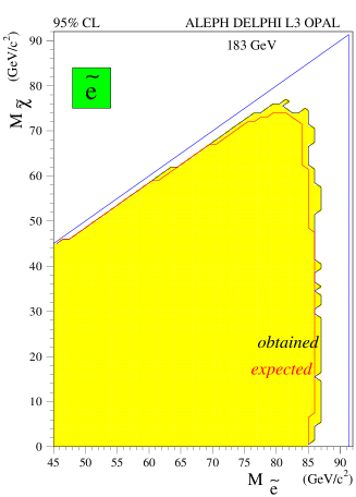
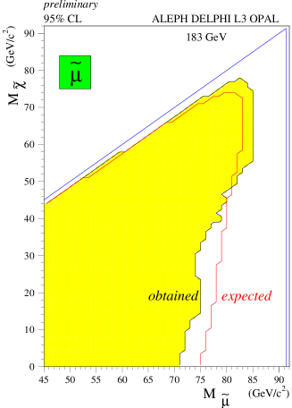
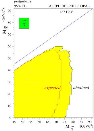
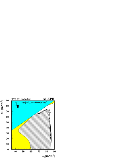
Figure 29: Combined exclusion contours for scalar electrons, muons and taus [126] as a function of the LSP mass and the limit for sleptons obtained by the ALEPH experiment [128] when combining all selectron and smuon searches up to 183 GeV (bottom–right).

	$\rm m_{\tilde{l}_{R}}\>$ lower limit ($\rm GeV/c^{2})$
	up to $\sqrt{s}=183$GeV
	Individual Limit (ADLO)	LEP combined
$\tilde{e}_{R}$ (Obs.)	79–83	85
(Exp.)	78–83	85
$\tilde{\mu}_{R}$ (Obs.)	55–62	71
(Exp.)	56–67	75
$\tilde{\tau}_{R}$ (Obs.)	45–63	75
(Exp.)	45–56	67

Table 11: Individual and LEP combined mass limits for $\tilde{e}_{R}$, $\tilde{\mu}_{R}$, $\tilde{\tau}_{R}$ up to $\sqrt{s}$ = 183 GeV for $\Delta M$ greater than 20 GeV, and assuming $\mbox{tan}\beta=2$ and $\mu=-200$ GeV for $\tilde{e}_{R}$.

Assuming a common scalar lepton mass at the GUT scale, the relation between the masses of right– and left–handed sleptons can be used to combine results of the searches for acoplanar leptons (muons, electrons together) [128] coming from the $\tilde{e}_{R}\tilde{e}_{L}$ process when the $\tilde{e}_{R}$ and the $\chi^{0}_{1}$ are mass degenerate ($\Delta M$ below 3 GeV). The result is shown in Fig. 29, for $\mbox{tan}\beta=2$ and $\mu=100$ GeV; this value of $\mu$ minimizes the product of cross section times branching fraction for the process $e^{+}e^{-}\rightarrow\tilde{e}_{R}\tilde{e}_{L}$ with $\tilde{e}_{L}\rightarrow e\chi^{0}_{1}$ for vanishing $\Delta M$. In this case, a scalar lepton mass limit of 65 $\rm GeV/c^{2}$ is set independently of $\Delta M$; this limit holds for higher values of $\mbox{tan}\beta$.

6.2.3 Scalar quarks

The squarks of the two first generations should be abundantly produced at the Tevatron which places already limits far above the kinematical reach of LEP2. Due to a large Yukawa coupling, the mass of one of the top squarks can be significantly smaller compared to those of the other scalar quarks; the large mixing between the left and right stops, proportional to $m_{t}$, leads to a large splitting of the two mass eigenstates. The lighter stop $\tilde{t}_{1}$ could be within the discovery range of LEP2. In addition, for large $\mbox{tan}\beta$ values ($\raisebox{-3.69899pt}{~{}\shortstack{$>$ \\ [-0.07cm] $\sim$}}~{}30$), the mixing angle in the sbottom sector can also be large and the lighter sbottom $\tilde{b}_{1}$ could also be within the reach of LEP2.

Stop and sbottom production at LEP proceed via $Z/\gamma$ exchange in the $s$–channel; the production cross sections depend on the squark mass and the squark mixing angle $\cos\theta_{q}$ and at $\cos\theta_{q}\sim 0.57$(0.39) the stop (sbottom) decouples from the $Z$–boson and the cross section is minimal; see section 5.5. The dominant decay modes of the $\tilde{t}_{1}$ are expected to be $\tilde{t}_{1}\rightarrow c\chi^{0}_{1}$ or $\tilde{t}_{1}\rightarrow b\tilde{\nu}l^{+}$; both of these decay modes have been searched for at LEP. The dominant decay mode of $\tilde{b}_{1}$ is expected to be $\tilde{b}_{1}\rightarrow b\chi^{0}_{1}$.

Under the assumption of R–parity conservation, the $\chi^{0}_{1}$ and the $\tilde{\nu}$ are invisible in the detector; thus stop or sbottom pair events are characterized by two acoplanar jets or two acoplanar jets plus two leptons, with missing energy. When the $\tilde{t}_{1}\rightarrow c\chi^{0}_{1}$ decay mode is dominant, the corresponding decay width is small enough for the top squark to hadronize into a colorless “stop hadron” before decaying; this feature has been implemented by the LEP experiments in their Monte Carlos. No excess of events was observed by any of the four LEP experiments [133]–[136], in the searches for stop and sbottom. Typical sensitivities obtained by the OPAL [136] experiment in the various channels, are listed in Tab. 12.

$m_{\tilde{t_{1}},\tilde{b_{1}}}=80$ GeV
$\sqrt{s}=183$ GeV
	$\tilde{t}_{1}\rightarrow c\chi^{0}_{1}$		$\tilde{b}_{1}\rightarrow b\chi^{0}_{1}$		$\tilde{t}_{1}\rightarrow bl\tilde{\nu}$
$\Delta M$ (GeV)	$\epsilon$ (%)	$N_{\rm back}^{\rm exp}$	$\epsilon$ (%)	$N_{\rm back}^{\rm exp}$	$\epsilon$ (%)	$N_{\rm back}^{\rm exp}$
7	23	1.97	37	1.97	11.8	1.07
15	58	1.97	61	1.97	64	2.05
80	37	1.97	31	1.97	58	2.05

Table 12: $\tilde{t}_{1}$ and $\tilde{b}_{1}$ efficiencies ($\epsilon$) and the number of events expected from the SM ($N_{\rm exp}$) obtained at $\sqrt{s}=183$ GeV by OPAL [136] as a function of $\Delta M$ for $m_{\tilde{q}}$ = 80 GeV.

All LEP results have been combined [126] and are summarized in Tab. 13 for $\Delta M$ greater than 15 GeV/c². Since a slight lack of events appears for sbottom searches, conservatively, the combination in this channel is done without any background subtraction. The LEP combined excluded regions in the plane ($m_{\chi_{1}^{0}},m_{\tilde{q}}$) are shown in Fig. 30.

	$\rm m_{\tilde{t}_{1}},m_{\tilde{b}_{1}}\>$ lower limits ($\rm GeV/c^{2})$
	up to $\sqrt{s}=183$GeV
	Individual Limit (ADLO)	LEP combined
	or AO only: ∗	obs  [exp]
$\tilde{t}_{1}\rightarrow c\chi^{0}_{1}$, $\rm cos\theta_{t}=1$	80–85	86 (85)
$\tilde{t}_{1}\rightarrow c\chi^{0}_{1}$, $\rm cos\theta_{t}=0.57$	72–81	83 (80)
$\tilde{t}_{1}\rightarrow b\tilde{\nu}l$, $\rm cos\theta_{t}=1$∗	84–85	87 (86)
$\tilde{t}_{1}\rightarrow b\tilde{\nu}l$, $\rm cos\theta_{t}=0.57$∗	80–82	85 (84)
$\tilde{b}_{1}\rightarrow b\chi^{0}_{1}$, $\rm cos\theta_{b}=1$	78–84	86 (83)
$\tilde{b}_{1}\rightarrow b\chi^{0}_{1}$, $\rm cos\theta_{b}=0.39$	45–68	75 (60)

Table 13: Individual and LEP combined mass limits for stop and sbottom up to $\sqrt{s}=183$ GeV for $\Delta M>15$ GeV, assuming maximal or minimal production cross sections.

At the Tevatron, top squarks can be directly pair produced or can be produced in the top quark decay mode $t\rightarrow\chi^{0}_{1}\tilde{t}_{1}$. The stop is searched for in the $\tilde{t}_{1}\rightarrow c\chi^{0}_{1}$ decay channel but also in the mode $\tilde{t}_{1}\rightarrow b\chi_{1}^{+}$ when kinematically allowed. Recently, the CDF [137] experiment has reported a higher limit on the $\tilde{t}_{1}$ mass of about 122 GeV/c² for $m_{\chi^{0}_{1}}$ lower than 50 GeV/c², the sensitivities in the low $\Delta M$ ranges are weak, due to the huge irreducible QCD background. The complementary domains excluded both at LEP2 and the Tevatron are shown in Fig. 30.

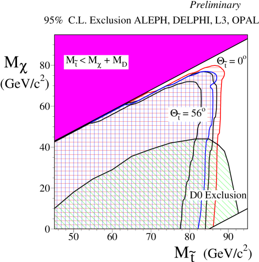
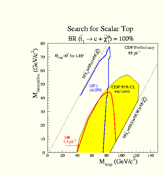
Figure 30: LEP2 (top) [126] and CDF (bottom) [137] exclusion domains in the plane ($m_{\chi^{0}_{1}},m_{\tilde{t}_{1}}$) from stop decay $\tilde{t}_{1}\rightarrow c\chi^{0}_{1}$ searches.

At hadron colliders, one expects the strongly interacting SUSY particles, gluinos and squarks, to be produced with the largest cross sections. Therefore the search for $\tilde{q}\tilde{q}$, $\tilde{q}\tilde{g}$ and $\tilde{g}\tilde{g}$ final states has been performed at the Tevatron by both the CDF [138] and D0 [139] collaborations. Depending on the mass hierarchy between squarks and gluinos, the subsequent decays will be $\tilde{q}\rightarrow q\tilde{g}$ or $\tilde{g}\rightarrow q\tilde{q}$; then decays of squarks and gluinos proceed according to $\tilde{q}\rightarrow q\chi_{1}^{0}$ and $\tilde{g}\rightarrow q\bar{q}\chi_{1}^{0}$ [the so called direct decays] while for sufficiently massive squarks and gluinos, the decays proceed through charginos $\chi^{\pm}_{1,2}$ or heavier neutralinos $\chi^{0}_{2,3,4}$, which in turn decay to quarks, leptons or neutrinos and one LSP [the so called cascade decays]. In the direct decays scenario, this leads to final states containing a significant number of jets and missing transverse energy carried away by the LSPs; it has to be noticed also that gluino decays yield on average one more jet than squarks decays. The cascade decays result in the production of a larger number of jets, with a reduced but still significant ${\rm E}_{\perp}/\hskip 0.28436pt$ and occasional production of leptons. The recent dilepton based SUSY search by CDF and D0 are sensitive to cascade decays.

No excess of data has be found at the two Tevatron experiments [138]–[139]; as an illustration, the CDF experiment for an integrated luminosity of 19 pb^-1, has selected 18 events in the three jets sample and 6 events in the four jets sample, these numbers are consistent with estimates of SM processes, respectively 33${}^{+12}_{-10}~{}({\rm stat})~{}^{+19}_{-12}~{}({\rm syst})$ and 8${}^{+4}_{-3}~{}({\rm stat})~{}^{+4}_{-4}~{}({\rm syst})$. The main background in this analysis comes from $W/Z$ + jets processes, top quark production and QCD multi–jet production in which the ${\rm E}_{\perp}/\hskip 0.28436pt$ originates from mismeasurement.

These searches yield lower limits on gluino and squark masses and the domains excluded by both experiments in the ($m_{\tilde{g}},m_{\tilde{q}}$) plane are shown in Figs. 31, where it is assumed that all but the top squark masses are degenerate. Assuming that squarks are heavier than the gluino, a lower limit on the common squark mass equal to 216 and 260 GeV/c² is set by the CDF and D0 collaborations, respectively. These limits do not depend on $\mbox{tan}\beta$ but hold only for large $\mu$ values [$\mu\raisebox{-3.69899pt}{~{}\shortstack{$>$ \\ [-0.07cm] $\sim$}}~{}200$ GeV or $\mu\raisebox{-3.69899pt}{~{}\shortstack{$<$ \\ [-0.07cm] $\sim$}}~{}-100$ GeV]. A tighter squark mass limit $m_{\tilde{q}}>267$ $\rm GeV/c^{2}$, using the dilepton channel, is set by D0; in this case however the result is more model dependent [charginos and heavy neutralinos have to decay leptonically, etc.].

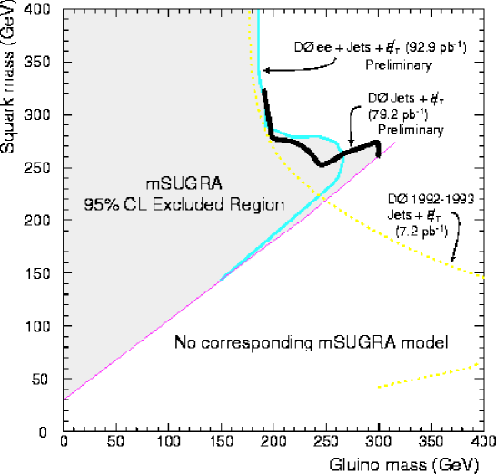
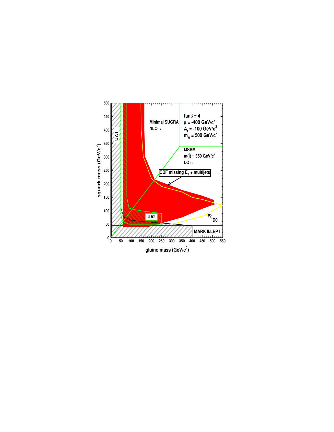
Figure 31: D0 (top) [139] and CDF (bottom) [138] exclusion domains in the plane ($m_{\tilde{g}},m_{\tilde{q}}$) from the multi–jet plus ${\rm E}_{\perp}/\hskip 0.28436pt$ or dileptons plus jets plus ${\rm E}_{\perp}/\hskip 0.28436pt$ searches at the Tevatron.

6.3. The gaugino sector

6.3.1 Gluinos

The gluino mass bounds derived from the $\tilde{q}\tilde{g}$ searches previously described, are respectively 173 and 187 GeV/c² for the CDF and D0 collaborations, for any squark mass. When one imposes an equal mass for squarks and gluinos, the limits become 216 and 260 $\rm GeV/c^{2}$ respectively, but are more model dependent.

In 1996, two small windows for very light gluinos [below 1.5 $\rm GeV/c^{2}$ and between 3 and 5 $\rm GeV/c^{2}$] remained unexcluded by any of the existing searches. Such light gluinos would modify the decay pattern of the SUSY particles considered; since with gluinos lighter than 5 $\rm GeV/c^{2}$, ${\rm E}_{\perp}/\hskip 0.28436pt$ becomes small and the usual jets + ${\rm E}_{\perp}/\hskip 0.28436pt$ signature is no more effective. However, resonant production of squarks would have a large cross section and, if squarks are not very heavy, broad peaks in the dijet mass distributions are expected. Comparison of the observed spectrum with theoretical estimates rules out light gluinos if squarks are lighter than about 600 $\rm GeV/c^{2}$ [127] . Such light gluinos would also affect the usual phenomenology of QCD at LEP, by changing the topology of four jet events via $g^{*}\rightarrow\tilde{g}\tilde{g}$ splitting; they would also contribute to the running of $\alpha_{s}$ as three additional flavors in leading order, up to mass effects. A full four–jet analysis carried out at LEP1 by ALEPH [140] excludes gluinos with masses smaller than $6.3~{}\rm GeV/c^{2}$.

6.3.2. Charginos and neutralinos

We now turn to the search for charginos and neutralinos at LEP2. At $e^{+}e^{-}$ colliders, charginos $\chi_{1}^{+}\chi_{1}^{-}$ (neutralinos $\chi_{i}^{0}\chi_{j}^{0}$ with ${\small i,j=1,\ldots,4}$ ordered by their masses) are pair–produced via $s$–channel $\gamma/Z$ ($Z$) boson and $t$–channel sneutrino $\tilde{\nu}$ (selectron $\tilde{e}$) exchange. When the masses of the sfermions are very large, the $\chi_{1}^{\pm}$ ($\chi_{j}^{0}$ with $j\geq 2$) states decay via an exchange of a virtual $W$ ($\rm Z$) boson as follows: $\chi_{1}^{\pm}\rightarrow\chi_{1}^{0}W^{*}\rightarrow\chi_{1}^{0}f\bar{f}^{\prime}$ ($\chi^{0}_{j}\rightarrow\chi_{k}^{0}Z^{*}\rightarrow\chi_{k}^{0}f\bar{f}$ with $k<j$). If the slepton and sneutrino masses are comparable to $M_{W}$ ($M_{Z})$ the charginos (next–to–lightest neutralinos) decay via virtual slepton or sneutrino exchange and the leptonic branching fraction is enhanced. Finally for slepton or sneutrino lighter than the chargino (next to lightest neutralino), the decay modes $\chi_{1}^{\pm}\rightarrow\tilde{l}^{\pm}\nu$ or $l^{\pm}\tilde{\nu}$ ($\chi^{0}_{j}\rightarrow\tilde{l}^{\pm}l^{\mp}$ or $\tilde{\nu}\nu$) become dominant. The radiative decays $\chi_{j}^{0}\rightarrow\chi_{k}^{0}\gamma$ are also possible via higher–order diagrams. For all LEP2 studies, the gluino is supposed to be heavy, otherwise the chargino decay patterns would be different, as reminded in the previous section.

The charginos and heavy neutralinos are searched for at LEP2 [141]–[146], in a first time within the large $m_{0}$ scenario, i.e large scalar fermion masses. In this case, charginos and neutralinos decay into the LSP accompanied by virtual $W$ and $Z$ bosons. The three possible final state topologies arising from the $W$ and $Z$ decays are: hadrons plus missing energy, acoplanar lepton pairs plus missing energy and mixed final state (hadrons plus leptons) plus missing energy. As explained before, signal topologies and the associated background sources depend on $\Delta M$. Therefore, for each topology, selections were optimized for four different $\Delta M$ ranges: the very low (3–5 GeV), the low (5–10 GeV), the medium (20–40 GeV) and the large ($\geq$ 50 GeV). In addition, the DELPHI experiment searched for topologies arising in the very small $\Delta M$ regime, with decays in flight and ISR tags [144]. Altogether a total of 27 events was observed by the four experiments with 25$\pm$5 expected from standard processes with efficiencies ranging from 5% to 65% depending on the analysis and the $\Delta M$ ranges as illustrated in Tab. 14.

$\rm M_{\chi_{1}^{\pm}}$=91 $\rm GeV/c^{2}$     $\chi_{1}^{\pm}\rightarrow\chi_{1}^{0}W^{*}$
$\Delta M$ (GeV)	$\epsilon$ (%)	$N_{\rm back}^{\rm exp}$	$N^{\rm obs}$
5	15	10.3 $\pm$ 1.1	8
20	55	17.4$\pm$ 1.1	18
60	14	17.4$\pm$1.1	18

Table 14: Typical efficiencies, number of expected and observed events obtained by the DELPHI experiment in the chargino searches at a c.m. energy of 183 GeV [143].

Depending on the neutralino–chargino field content, one distinguishes the following cases for the determination of the lower limits on neutralino–chargino masses:

– Higgsino–like $\chi_{2}^{0}$ and $\chi_{1}^{\pm}$ ($M_{2}\gg|\mu|$): in this case, the production cross sections do not depend on the scalar lepton masses, and $\Delta M$ is low and decreases with increasing $M_{2}$. Consequently, the limits on the masses of the next–to–lightest neutralino and the lightest chargino decrease with $M_{2}$. The present LEP2 combined [126] limit on the chargino mass is shown in Fig. 32 (top left) turning into a limit on the chargino mass of 63 $\rm GeV/c^{2}$ for $\Delta M\geq 3~{}\rm GeV/c^{2}$. The DELPHI experiment has excluded regions for lower $\Delta M$ ranges as depicted in Fig. 32(bottom). Masses lower than 80 $\rm GeV/c^{2}$ are excluded by all LEP experiments for the next–to–lightest neutralino $\chi_{2}^{0}$ assuming $M_{2}$ less than 1500 $\rm GeV/c^{2}$. This limit holds only for higgsino–like $\chi^{0}_{2}$, since the coupling to the $Z$–boson vanishes for gaugino–like neutralinos.

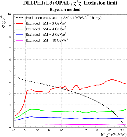
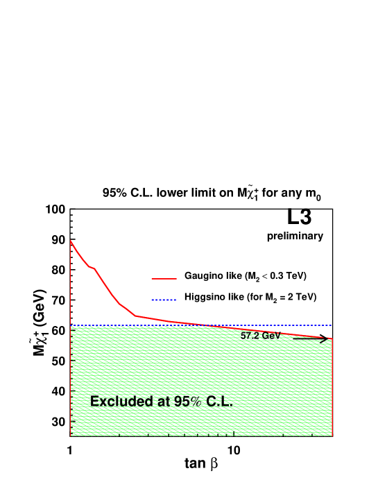
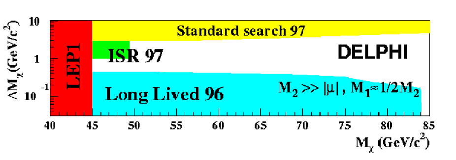
Figure 32: Top left: LEP combined [126] lower limit on the chargino mass for different $\Delta M$ values at c.m. energies up to 183 GeV. Top right: lower limit on the chargino mass for different field content, as a function of $\mbox{tan}\beta$, by the L3 experiment [145]. Bottom: excluded domains in the plane ($m_{\chi^{\pm}_{1}},\Delta M$) in the very low $\Delta M$ range obtained by DELPHI [144] at a c.m. energy up to 183 GeV.

– Gaugino–like chargino ($|\mu|\gg M_{2}$): the cross section depends strongly on the scalar neutrino mass. For $50\leq m_{\tilde{\nu}}\leq 80$ $\rm GeV/c^{2}$ the destructive interference term reduces the cross section by one order of magnitude compared to what is expected for $m_{\tilde{\nu}}\geq 300$ $\rm GeV/c^{2}$. When the two body decay $\chi_{1}^{\pm}\rightarrow l^{\pm}\tilde{\nu}$ is dominant, the relevant $\Delta M$ becomes equal to $m_{\chi_{1}^{\pm}}-m_{\tilde{\nu}}$. Therefore, the limit on the chargino mass will depend clearly on the $m_{\tilde{\nu}}$ value. For large $m_{\tilde{\nu}}$ values ($\geq$ 300 $\rm GeV/c^{2}$), the situation is the ideal one: we benefit there from the best detection sensitivity and the highest cross section production. This is the reason why the kinematical limit is reached with only a few $~{}{\rm pb}^{-1}$. Up to now, including the recent 189 GeV data, LEP experiments exclude a chargino mass below 94.3 $\rm GeV/c^{2}$, irrespective of $\mbox{tan}\beta$. Extending the study to all $m_{\tilde{\nu}}$ values where the chargino leptonic decay is enhanced for low slepton masses, dedicated analyses then were developed by the LEP experiments. However, it appears that the chargino cannot be directly detected when it is degenerate in mass with the sneutrino since the soft leptons produced in the final state escape detection. In this case, the LEP1 limit of 45 $\rm GeV/c^{2}$ remains, that is deduced from the $Z$–boson total decay width measurement which is insensitive to the chargino decay pattern. Recently, this limit has been improved in two independent ways: $(i)$ the ALEPH experiment, excludes $m_{\chi_{1}^{\pm}}$ below 51 $\rm GeV/c^{2}$ by measuring the invisible $W$–boson width, within some model assumptions [142]; and $(ii)$ the L3 experiment [145] exploits the complementarity of the scalar lepton searches, excluding chargino masses below 57.2 $\rm GeV/c^{2}$ irrespective of $\mbox{tan}\beta$ and $m_{0}$, as depicted in Fig. 32 (top right).

At the Tevatron, charginos and neutralinos may be produced directly in the annihilation process $qq\rightarrow\chi_{2}^{0}\chi_{1}^{\pm}$ or in the decays of heavier squarks as mentioned before. They are searched for in the leptonic decays [mainly assuming the decays $\chi_{1}^{\pm}\rightarrow l^{\pm}\nu\chi_{1}^{0}$ and $\chi_{2}^{0}\rightarrow l^{+}l^{-}\chi_{1}^{0}$]; see section 5.3. The requirement of three leptons in the final state reduces backgrounds to a very small level but is efficient for the signal only in peculiar cases. Therefore, charginos and neutralinos may be discovered at the Tevatron above the kinematical reach of LEP2, but no robust limits can be derived and the results reported today are not competitive with the LEP bounds.

6.3.3 Neutralino LSP

Finally, let us discuss the neutralino–LSP mass limits. Since the neutralino $\chi_{1}^{0}$ is the LSP and escapes detection, direct searches for the LSP neutralino cannot be performed at LEP2. However, indirect limits have been derived from the constraints on chargino–neutralino and slepton searches. As detailed previously, the limits depend on the slepton masses, in particular on $m_{\tilde{\nu}}$.

– Large sneutrino mass: For high $\mbox{tan}\beta$ values, the chargino search provides the most stringent bound on $m_{\chi_{1}^{0}}$. For $\mbox{tan}\beta$ values below 2, the neutralino searches including the processes $e^{+}e^{-}\rightarrow\chi_{1}^{0}\chi_{3}^{0},\,\chi_{1}^{0}\chi_{4}^{0},\,\chi_{2}^{0}\chi_{3}^{0}$ but also the radiative decays $\chi_{2}^{0}\rightarrow\chi_{1}^{0}\gamma$, exclude additional regions of the parameter space (mixed region). The LEP1 exclusion limits still play some role, due to the fact that the neutralino search is limited in the region near the point where the $\chi_{1}^{0}$ mass limit is set by the value of the coupling to the $Z$–boson rather than by kinematics. The lower limit obtained for $m_{\chi_{1}^{0}}$ as a function of $\mbox{tan}\beta$ and for heavy sleptons is displayed in Fig. 33 for LEP center–of–mass energies increasing from 91.5 up to 183 GeV. A summary of all limits [141]–[146] obtained both up to 183 GeV and more recently to 189 GeV is listed in Tab. 15.

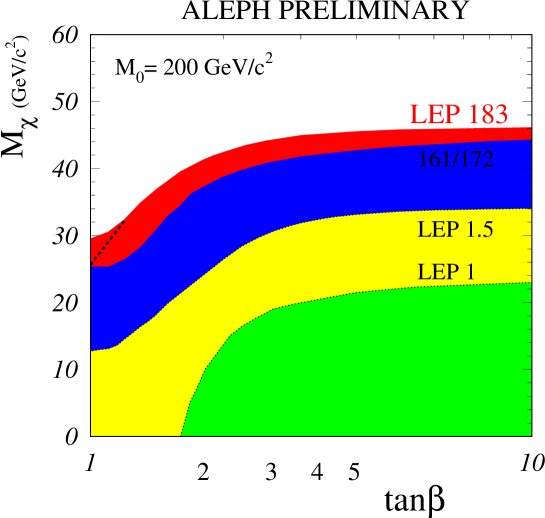
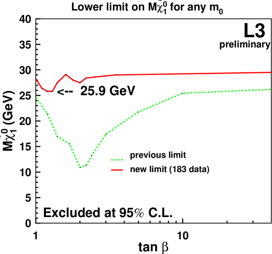
Figure 33: Top: ALEPH [141] lower limit on the LSP mass as a function of $\mbox{tan}\beta$, for large slepton masses, at c.m. energies up to 183 GeV. Bottom: Lower limit on the LSP mass as a function of $\mbox{tan}\beta$, for any slepton mass obtained by L3 [145] at c.m. energies up to 183 GeV.

– Any sneutrino mass: For lower slepton masses, as already discussed, the constraints in the chargino–neutralino sectors are weaker and the limits on $m_{\chi_{1}^{0}}$ therefore degradate. Constrains on $m_{\chi_{1}^{0}}$ have been obtained by all LEP experiments with a systematic scan of the MSSM parameter space, as a function of $\mbox{tan}\beta$ for all $m_{0}$ values, as depicted in the bottom of Fig. 33. For low $\mbox{tan}\beta$ values ($\leq 1.6)$ the minimum allowed value for $m_{\chi_{1}^{0}}$ is found in the parameter space where the production cross section for charginos is minimal [$m_{\tilde{\nu}}\sim$ 90 $\rm GeV/c^{2}$ in the mixed region $\mu\sim-70~{}\rm GeV/c^{2}$] [143]–[146] and the heavy neutralino $\chi_{3,4}^{0}$ are mostly invisible while for higher $\mbox{tan}\beta$ values ($\geq 2)$ the lower $\chi_{1}^{0}$ mass limit is found in the parameter space region where the chargino and sneutrino mass difference is small and where the next–to–lightest neutralinos $\chi_{2}^{0}$ decay invisibly. The exclusion limit came only from slepton searches; it is localized in the deep gaugino–like region for charginos ($\mu\leq-400~{}\rm GeV/c^{2}$) [141]. The limits obtained by each experiment are listed in Tab. 15 as well as the MSSM parameter ranges used in the scan. The most recent limit on the $\tilde{e}$ mass obtained with 189 GeV data by ALEPH [141] allows to set the best absolute limit on the LSP mass of 28 $\rm GeV/c^{2}$, which can be turned into an absolute limit on $M_{2}$.

	$m_{\chi_{1}^{0}}>$ ($\rm GeV/c^{2})$
	up to 183 Gev	up to 189 GeV
Large $m_{0},\mbox{tan}\beta\geq$ 1	$\sim$ 30.5   (ADLO)	$\sim$ 32.5   (AO)
Any $m_{0},\mbox{tan}\beta\geq$1
A     $\mu$ up to $-2000$ $\rm GeV/c^{2}$	26∗	28
D     $\mu$ up to $-200$ $\rm GeV/c^{2}$	23.4
L    $\mu$ up to $-500$ $\rm GeV/c^{2}$	25.9
O    $\mu$ up to $-500$ $\rm GeV/c^{2}$	25.4

Table 15: Indirect individual mass limits for the LSP $\chi_{1}^{0}$ up to $\sqrt{s}$ = 183, 189 GeV for large $m_{0}$ or any $m_{0}$. In the latter case, the minimum value (^∗) for ALEPH experiment is found in the deep–gaugino region (up to 183 GeV data) while other experiments found the minimum in the mixed region.

6.4 Summary and Bounds on the MSSM parameters

The summary of the bounds on the SUSY particles obtained at LEP2 and the Tevatron are listed in Tab. 16. We also indicate the parameter ranges for which these limits hold.

Particle	Assumptions	Lower limit	Experimental
		($\rm GeV/c^{2}$)	sources
h	$\mbox{tan}\beta\geq$0.8	78.8	LEP2 Comb.
A	$\mbox{tan}\beta\geq$0.8	79.1	LEP2 Comb.
H±	Br($\rm H\rightarrow c\bar{s})$ + Br($\rm H\rightarrow c\bar{s}$)=1	68	LEP2 Comb.
	any $\mbox{tan}\beta$
	$\mbox{tan}\beta\leq$1.1 or $\mbox{tan}\beta\geq$40	100	CDF/D0
$\tilde{e}_{R}$	Br($\tilde{e}_{R}$ $\rightarrow e\chi_{1}^{0}$)=1, $\Delta$M$\geq 20~{}\rm GeV/c^{2}$	85	LEP2 Comb.
	Br($\tilde{e}_{R}$ $\rightarrow e\chi_{1}^{0}$)=1, $\mbox{tan}\beta\geq$2	65	LEP2
$\rm\tilde{\mu}_{R}$	BR($\rm\tilde{\mu}_{R}$ $\rightarrow\mu\chi_{1}^{0}$ )=1, $\Delta$ M $\geq$ 20 $\rm GeV/c^{2}$	71	LEP2 Comb.
$\rm\tilde{\tau}_{R}$	BR($\rm\tilde{\tau}_{R}$ $\rightarrow\tau\chi_{1}^{0}$)=1, $\Delta$ M $\geq 20~{}\rm GeV/c^{2}$	75	LEP2 Comb.
$\tilde{\nu}$		43	LEP1 – Z width
$\rm\tilde{t}_{1}$	BR($\rm\tilde{t}_{1}$ $\rightarrow c\chi_{1}^{0}$)=1, $\Delta$ M $\geq$ 15 $\rm GeV/c^{2}$	83	LEP2 Comb.
	BR($\rm\tilde{t}_{1}$ $\rightarrow\nu l\chi_{1}^{0}$ )=1, $\Delta$ M $\geq$ 15 $\rm GeV/c^{2}$	85	LEP2 Comb.
	BR($\rm\tilde{t}_{1}$ $\rightarrow c\chi_{1}^{0}$ )=1, ${\rm LEP2;~{}m_{\chi_{1}^{0}}\leq 50~{}GeV}$	122	CDF
$\rm\tilde{b}_{1}$	BR($\rm\tilde{b}_{1}$ $\rightarrow b\chi_{1}^{0}$ )=1, $\Delta$ M $\geq 15~{}\rm GeV/c^{2}$	75	LEP2 Comb.
$\rm\tilde{q}$	$\rm m_{\tilde{q}}\geq m_{\tilde{g}}$	216	CDF
	$\rm m_{\tilde{q}}\geq m_{\tilde{g}}$	260	D0
$\rm\tilde{g}$	$\mu\leq-100$ or $\mu\geq 200~{}\rm GeV/c^{2}$	173	CDF
	$\mu\leq-100$ or $\mu\geq 200~{}\rm GeV/c^{2}$	187	D0
$\chi^{\pm}_{1}$	Higgsino $\Delta$M $\geq 3~{}\rm GeV/c^{2}$	63	LEP2 Comb.
	Gaugino $\rm m_{0}$ $\geq 200~{}\rm GeV/c^{2}$	94.3	LEP2∗
	Gaugino any $\rm m_{0}$	57.2	LEP2
$\chi^{0}_{1}$	Large $\rm m_{0}$	32.5	LEP2∗
	Any $\rm m_{0}$	28	LEP2∗

Table 16: Summary of lower mass limits obtained at the Tevatron and at LEP2 up to $\sqrt{s}$ = 183, 189 GeV [^∗ at which just a small fraction of data has been used].

The limits can be turned into bounds on the cMSSM parameters; as an example, at the Tevatron, the excluded region in the ($m_{\tilde{g}},m_{\tilde{q}}$) plane is translated in the plane ($m_{0},m_{1/2}$) for different $\mbox{tan}\beta$ values, see Fig. 34 (top). Similarly, LEP experiments have derived from chargino/neutralino searches excluded contours in the plane ($\mu,M_{2}$) for different $m_{0}$, $\mbox{tan}\beta$ values as illustrated on Fig. 35; in particular the clear complementarity of the searches for neutralinos and charginos is visible for the low $\mbox{tan}\beta$ regime. Moreover, the combination of the gaugino and the slepton searches allowed to exclude regions of parameters in the plane ($m_{0},m_{1/2}$) and to derive an absolute limit on $M_{2}$ of 47 $\rm GeV/c^{2}$ independently of $m_{0}$, $\mu$ and $\mbox{tan}\beta$.

The low values of the parameter $\mbox{tan}\beta$ are already constrained, for a given set of parameters, by the Higgs boson searches performed at LEP2. The combination of results obtained at the Tevatron and at LEP2, allow to set more robust and stringent constraints for the low $\mbox{tan}\beta$ regime, as already tested in Ref. [118] and illustrated in Fig. 26. Finally constraints form the Higgs sector and the other SUSY particle sector, could be combined to derive improved bounds on the cMSSM parameters; a first attempt has been done in Ref. [147] when combining Higgs and SUSY limits obtained at LEP2 for a c.m. energy up to 172 GeV. It was shown that the interplay between Higgs and stop mass lower limits allows $m_{1/2}$ to be constrained for low values of $\mbox{tan}\beta$ and $m_{0}$: for small (large) mixing, the Higgs (stop) mass limit provides the most effective constraint. On the bottom of Fig. 34, one can see clearly how the lower limit on the LPS is strengthened by taking the Higgs information into account for small $\tan\beta$.

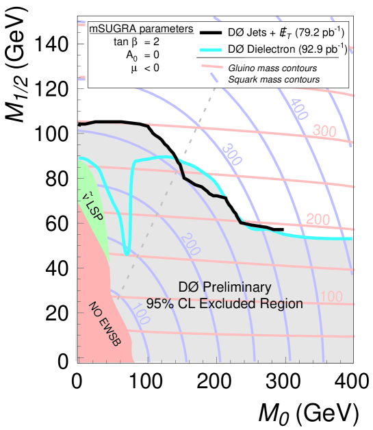
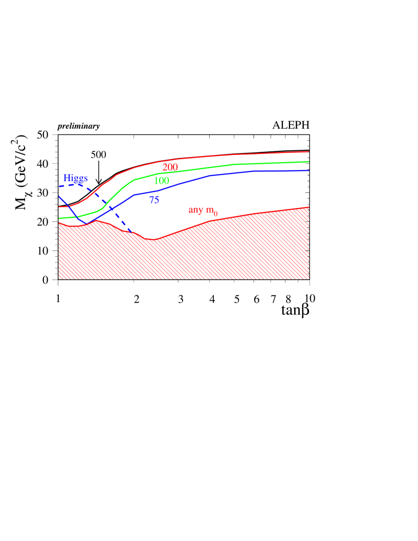
Figure 34: Top: D0 [139] exclusion contours in the plane ($m_{0},m_{1/2}$) from the multi–jet plus ${\rm E}_{\perp}/\hskip 0.28436pt$ or dileptons plus jets plus ${\rm E}_{\perp}/\hskip 0.28436pt$ searches. Bottom: Lower limit on the mass of the lightest neutralino as a funtion of $\mbox{tan}\beta$ for a series of $m_{0}$ values by the ALEPH experiment [147] for a c.m. energy up to 172 GeV. The dashed curve shows the result coming from the Higgs constraints for $m_{0}$=75 $\rm GeV/c^{2}$

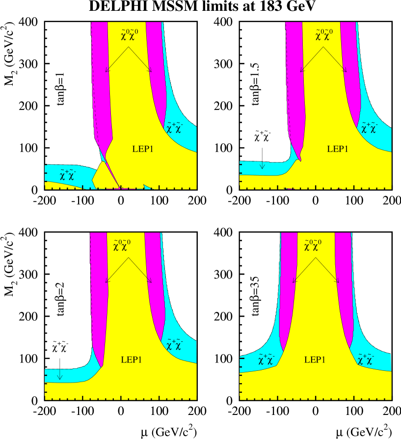
Figure 35: Regions in the ($\mu$,$M_{2}$) plane excluded by DELPHI [143] for different values of $\mbox{tan}\beta$, assuming large $m_{0}$. The lightly shaded areas are those excluded by lower energy LEP1 results. The intermediate shading shows regions excluded by the chargino search at 183 GeV. The darkly shaded areas show the regions excluded by the neutralino searches at these energies.

References

- [1] This was, in a preliminary version, since already some time on the Web page of our working group, http://www.lpm.univ-montp2.fr:7082/ djouadi/gdr.html.
- [2] C. Le Mouël and G. Moultaka, Note GDR–S–002 and Nucl. Phys. B518 (1998) 3.
- [3] C. Le Mouël and G. Moultaka, to appear.
- [4] G. Auberson and G. Moultaka, to appear.
- [5] J.L. Kneur and G. Moultaka, Note GDR–S–14 and hep–ph/9807336.
- [6] A. Djouadi, J.L. Kneur and G. Moultaka, Note GDR–S–17.
- [7] A. Djouadi, Note GDR–S–006 and hep-ph/9806315 and Phys. Lett. B435 (1998) 101.
- [8] A. Djouadi, J.L. Kneur and G. Moultaka, Note GDR–S–003 and Phys. Rev. Lett. 80 (1998) 1830.
- [9] A. Djouadi, Note GDR–S–013.
- [10] F. Borzumati and A. Djouadi, Note GDR–S–011 and hep–ph/9806301.
- [11] A. Djouadi, Note GDR–S–012.
- [12] A. Djouadi, J.L. Kneur and G. Moultaka, to appear.
- [13] J. Layssac, F.M. Renard and C. Verzegnassi, Note GDR–S–001.
- [14] S.Y. Choi, A. Djouadi, H. Dreiner, J. Kalinowski and P.M. Zerwas, hep-ph/9806279.
- [15] M.B. Causse, G. Montarou, G. Moultaka and E. Nuss, Note GDR–S–15.
- [16] S. Muanza, Note GDR–S–020.
- [17] Y. Mambrini, C. Boehm and A. Djouadi, Note GDR–S to appear.
- [18] Ph. Gris, Note GDR–S–016 and PhD thesis DAPNIA/SPP 98–1001.
- [19] S. Rosier–Lees, Note GDR–S to appear.
- [20] Supersymmetry and Supergravity by J. Wess and J. Bagger, Princeton Series in Physics.
- [21] For reviews on the MSSM, see: P. Fayet and S. Ferrara, Phys. Rep. 32 (1977) 249; H.P. Nilles, Phys. Rep. 110 (1984) 1; R. Barbieri, Riv. Nuov. Cim. 11 (1988) 1; R. Arnowitt and Pran Nath, Report CTP-TAMU-52-93; M. Drees and S. Martin, CLTP Report (1995) and hep-9504324; S. Martin, hep-ph9709356; J. Bagger, Lectures at TASI-95, hep-ph/9604232.
- [22] H. E. Haber and G. Kane, Phys. Rep. 117 (1985) 75.
- [23] For a review on the Higgs sector of the MSSM, see J.F. Gunion, H.E. Haber, G.L. Kane and S. Dawson, “The Higgs Hunter’s Guide”, Addison–Wesley, Reading 1990.
- [24] N. Sakai, Z. Phys. C11 (1981) 153; S. Dimopoulos and H. Georgi, Nucl. Phys. B193 (1981) 150; E. Witten, Nucl. Phys. B231 (1984) 419.
- [25] K. Inoue, A. Komatsu and S. Takeshita, Prog. Theor. Phys 68 (1982) 927; (E) 70 (1983) 330.
- [26] P. Fayet, Phys. Lett. 69B (1997) 489; G. Farrar and P. Fayet, Phys. Lett. 76B (1978) 575.
- [27] P. Fayet and J. Iliopoulos, Phys. Lett. 51B (1974) 461; L. O’Raifeartaigh, Nucl. Phys. B96 (19975) 331.
- [28] A.H Chamseddine, R. Arnowitt and P. Nath, Phys. Rev. Lett. 49 (1982) 970; R. Barbieri, S. Ferrara and C.A Savoy, Phys. Lett. B119 (1982) 343; L. Hall, J. Lykken and S. Weinberg, Phys. Rev. D27 (1983) 2359.
- [29] Y. Suzuki for the Super–Kamiokande, talk given at “neutrinos 98”, Takayama (Japan), June 1998.
- [30] S. Dimopoulos and D. Sutter, Nucl. Phys. B452 (1995) 496; see also the discussion given by H.E. Haber, hep-ph/9709450.
- [31] Report of the working group “Saveurs”.
- [32] See for instance, G. Anderson et al. hep-ph/9609457 and references therein.
- [33] J. Ellis , S. Kelley and D.V. Nanopoulos, Phys. Lett. B260 (1991) 131; U. Amaldi, W. de Boer and H. Fürstenau, Phys. Lett. B260 (1991) 447; P. Langacker and M. Luo, Phys. Rev.D 44 (1991) 817; C. Giunti, C.W. Kim and U.W. Lee, Mod. Phys. Lett. A6 (1991) 1745.
- [34] M.S. Chanowitz, J. Ellis and M.K. Gaillard, Nucl. Phys. B128 (1977) 506.
- [35] V. Barger, M.S. Berger, R.J. Phillips, Phys. Lett. B314 (1993) 351; M. Carena, S. Pokorski and C. Wagner, Nucl. Phys. B406 (1993) 59.
- [36] M. Brhlik and G.L. Kane, Report UM-TH-98-07, hep-ph/9803391
- [37] See for instance, R. Arnowitt and P. Nath, Phys. Rev. D56 (1997) 2820 and 2833.
- [38] For a recent review, see M. Carena and C.E.M. Wagner, hep-ph/9704347.
- [39] S. Coleman and E. Weinberg, Phys. Rev. D 7 (1973) 1888.
- [40] M. Bando, T. Kugo, N. Maekawa and H. Nakano, Phys. Lett. B 301 ( 1993).
- [41] L. Ibañez and G.G. Ross Phys. Lett. B110 (1982) 227; L. Alvarez-Gaumé, J.Plochinski and M.B. Wise, Nucl. Phys. B250 (1983) 495; J. Ellis et al. Phys. Lett. B125 (1983) 2275; N.K. Falck, Z. für Phys. C30 (1986) 247; see also for instance R. Arnowitt and P. Nath in [21] and references therein.
- [42] L.E. Ibáñez and C. Lopéz, Phys.Lett. 126B (1983) 54; Nucl. Phys. B233 (1984) 511; ibid. B256 (1985) 218.
- [43] F.G. Floratos, G.K. Leontaris, Phys.Lett. B336 (1994) 194.
- [44] See for instance, “Ordinary Differential Equations”, by G.M. Murphy, Van Nostrand Reinhold Company, ed. (1996).
- [45] J.F. Gunion and H.E. Haber, Nucl. Phys. B272 (1986) 1 and erratum hep-ph/9301205.
- [46] M. El Kheishen, A. Shafik and A. Aboshousha, Phys. Rev. D45 (192) 4345.
- [47] J. Ellis and S. Rudaz, Phys. Lett. B128 (1983) 248; M. Drees and K. Hikasa, Phys. Lett. B252 (1990) 127.
- [48] Y. Okada, M. Yamaguchi and T. Yanagida, Prog. Theor. Phys. 85 (1991) 1; H. Haber and R. Hempfling, Phys. Rev. Lett. 66 (1991) 1815; J. Ellis, G. Ridolfi and F. Zwirner, Phys. Lett. 257B (1991) 83; R. Barbieri, F. Caravaglios and M. Frigeni, Phys. Lett. 258B (1991) 167; M. Drees and M.M. Nojiri, Phys. Rev. D45 (1992) 2482; R. Hempfling and A. Hoang, Phys. Lett. B331 (1994) 99; S. Heinemeyer, W. Hollik and G. Weiglein, hep-ph/9803277.
- [49] M. Carena, M. Quiros and C.E.M. Wagner, Nucl. Phys. B461 (1996) 407; H. Haber, R. Hempfling and A. Hoang, Z. Phys. C75 (1997) 539.
- [50] V. Barger, M.S. Berger, A.L. Stange and R.J.N. Phillips, Phys. Rev. D45 (1992) 4128; A. Brignole and F. Zwirner, Phys. Lett. B299 (1993) 72.
- [51] CMS Collaboration (S. Abdullin et al.), CMS-NOTE-1998-006, hep-ph/9806366; D. Denegri, W. Majerotto and L. Rurua, CMS-NOTE-1997-094, hep-ph/9711357; I. Hinchliffe et al., Phys. Rev. D55 (1997) 5520.
- [52] See the discussion given by S. Martin in Ref. [21].
- [53] See the report of the working group “Outils”.
- [54] SUBH: subroutine by M. Carena, M. Quiros and C.E.M. Wagner, based on Phys. Lett. B335 (1995) 209.
- [55] Particle Data Group, Phys. Rev. D54, 1 (1996); for a recent collection of limits on SUSY and Higgs particles, see section 6.
- [56] W. Press, S. Teuksolsky, W. Vetterling and B. Flannery, Numerical Recipes: the Art of Scientific Computing, Cambridge Univ. Press 1988.
- [57] M. Carena, P.M. Zerwas et al., Higgs Physics at LEP2, CERN Yellow Report CERN-96-01, hep-ph/9602250.
- [58] Report of the Tev2000 study group on ”Future Electroweak Physics at the Tevatron”, D. Amidei and R. Brock, eds. (1995).
- [59] ATLAS Collaboration, Technical Proposal, Report CERN–LHCC 94–43; CMS Collaboration, Technical Proposal, Report CERN–LHCC 94–38.
- [60] D. Froidevaux, Z. Kunszt and J. Stirling [conv.] et al., in Proceedings of the Large Hadron Collider Workshop, Aachen 1990, Report CERN 90–10, Vol. II; See also the Rapporteurs talks by G. Altarelli and D. Denegri in the same proceedings; For a recent review on Higgs physics at the LHC, see e.g.: J.F. Gunion et al., hep-ph/9602238, Proceedings of the Snowmass 96 Workshop; M. Spira, Habilitation thesis, hep-ph/9705337.
- [61] E. Accomando et al., LC CDR Report DESY 97-100 Physics Reports 299 (1998) 1; S. Kuhlman et al., NLC ZDR Design Group and the NLC Physics Working Group, SLAC–R–0485; A. Djouadi, Int. J. Mod. Phys. A10 (1995) 1.
- [62] See for instance H.E. Haber, CERN-TH/95-109 and hep-ph/9505240.
- [63] H. Georgi et al., Phys. Rev. Lett. 40 (1978) 692.
- [64] A. Djouadi, M. Spira and P.M. Zerwas, Phys. Lett. B264 (1991) 440; S. Dawson, Nucl. Phys. B359 (1991) 283; M. Spira, A. Djouadi, D. Graudenz and P.M. Zerwas, Nucl. Phys. B453 (1995) 17; S. Dawson, A. Djouadi and M. Spira, Phys. Rev. Lett. 77 (1996) 16.
- [65] S.L. Glashow, D.V. Nanopoulos and A. Yildiz, Phys. Rev. D18 (1978) 1724; Z. Kunszt, Z. Trocsanyi and W.J. Stirling, Phys. Lett. B271 (1991) 247.
- [66] Z. Kunszt, Nucl. Phys. B247 (1984) 339; J.F. Gunion, Phys. Lett. B253 (1991) 269; W. Marciano and F. Paige, Phys. Rev. Lett. 66 (1991) 2433.
- [67] J. Dai, J.F. Gunion and R. Vega, Phys. Rev. Lett 71 (1993) 2699; D. Froidevaux and E. Richter-Was, Z. Phys. C67 (1995) 213.
- [68] D.R.T. Jones and S.T. Petcov, Phys. Lett. B84 (1979) 440; R.N. Cahn and S. Dawson, Phys. Lett. B136 (1984) 196; K. Hikasa, Phys. Lett. B164 (1985) 341; G. Altarelli, B. Mele and F. Pitolli, Nucl. Phys. B287 (1987) 205; W. Kilian, M. Krämer and P.M. Zerwas, Phys. Lett. B373 (1996) 135.
- [69] For the Higgs boson decay branching ratios, see e.g. A. Djouadi, hep–ph/9703230 and hep–ph/9710439.
- [70] D. Froidevaux et al., ATLAS internal note PHYS-no-74 (1995).
- [71] A. Djouadi, V. Driesen, W. Hollik and J.I. Illana, Eur. Phys. J. C1 (1998) 149.
- [72] A. Djouadi, J. Kalinowski and M. Spira, Comput. Phys. Commun. 108 (1998) 56.
- [73] See for instance, G. Altarelli, hep-ph/9611239.
- [74] Z. Kunszt, S. Moretti and W.J. Stirling, Z. Phys. C74 (1997) 479.
- [75] CTEQ Collaboration, Phys. Rev. D51 (1995) 4763.
- [76] F. Abe et al. (CDF Collaboration), Phys. Rev. Lett. 79 (1997) 357.
- [77] F. Borzumati and C. Greub, Phys. Rev. D58 (1998) 074004 and hep–ph/9809438; F. Borzumati and C. Greub, hep–ph/9810240.
- [78] D. Antreasyan et al. (Cristal Ball Coll.), Phys. Lett. B251 (1990) 204.
- [79] J. Ellis, M. K. Gaillard and D.V. Nanopoulos, Nucl. Phys. B106 (1976) 292; B.W. Lee, C. Quigg and H.B. Thacker, Phys. Rev. D16 (1977) 1519; J.D. Bjorken, Proceedings of Summer Institute on Particle Physics, SLAC Report 198 (1976); B.L. Ioffe and V.A. Khoze, Sov. J. Part. Nucl. 9 (1978) 50.
- [80] J. Gunion et al., Phys. Rev. D38 (1988) 3444; A. Djouadi, J. Kalinowski and P.M. Zerwas, Z. Phys. C57 (1993) 569; A. Djouadi, hep-ph/9406433.
- [81] A. Djouadi, J. Kalinowski and P. M. Zerwas, Z. Phys. C54 (1992) 255 and Mod. Phys. Lett. A7 (1992) 1765.
- [82] For the SM case: G. Gounaris, D. Schildknecht and F. Renard, Phys. Lett. B83 (1979) 191 and (E) 89B (1980) 437; V. Barger and T. Han, Mod. Phys. Lett. A5 (1990) 667; V. Ilyin, et al., Report KEK CP–030; F. Boudjema and E. Chopin, Z. Phys. C73 (1996) 85.
- [83] For the analysis in the MSSM, see: A. Djouadi, H.E. Haber and P.M. Zerwas, Phys. Lett. B375 (1996) 203; P. Osland and P.N. Pandita, hep-ph/9806351.
- [84] For the SM case, see: A. Barroso, J. Pulido, J. C. Romao, Nucl. Phys. B267 (1985) 509; A. Abbasabadi, D. Bowser-Chao, D. A. Dicus and W. A. Repko, Phys. Rev. D52 (1995) 3919;
- [85] For the analysis in the SM and MSSM, see: A. Djouadi, V. Driesen, W. Hollik and J. Rosiek, Nucl. Phys. B491 (1997) 68.
- [86] A. Djouadi, J. L. Kneur and G. Moultaka, in preparation.
- [87] I.F. Ginzburg, G. Kotkin, V. Serbo and V.I. Telnov, Nucl. Instrum. Meth. 205 (1983) 47 and 219 (1984) 5; V.I. Telnov, Nucl. Instrum. Meth. A294 (1990) 72 and A335 (1995) 3.
- [88] T. Ohl, Comput. Phys. Commun.101 (1997) 269.
- [89] G. Bélanger, F. Boudjema, T. Kon and V. Lafage, hep-ph/9811334.
- [90] M. Consoli and W. Hollik, in “ Physics at LEP1”, Vol. 1, p. 7, G. Altarelli, R. Kleiss, C. Verzegnassi eds.
- [91] F.M. Renard and C. Verzegnassi, Phys. Rev. D52 (1995) 1369 and D53 (1996) 1290.
- [92] See e.g. the discussion given in: “Physics at LEP2”, Proceedings CERN 96-01, G. Altarelli, T. Sjostrand and F. Zwirner eds.
- [93] See for instance, A. Bartl, H. Fraas and W. Majerotto, Z. Phys. C30 (1986) 441.
- [94] M. Chen, C. Dionisi, M. Martinez and X. Tata, Phys. Ret. 159 (1998) 203; A. Leike, Int. J. Mod. Phys. A3 (1988) 2895; M.A. Diaz and S.F. King, Phys. Lett. B349 (1995) 105; B373 (1996) 100; J.L. Feng and M.J. Strassler, Phys. Rev. D51 (1995) 4461 and D55 (1997) 1326; G. Moortgat-Pick, H. Fraas, A. Bartl and W. Majerotto, hep-ph/9804306.
- [95] S. Katsanevas et al., contribution of the group “Outils” to this report.
- [96] S.Y. Choi et al., hep-ph/9812236.
- [97] H. Baer et al., Phys. Rev. D35 (1987) 1598 and Phys. Rev. D36 (1987) 96.
- [98] S. Dawson, E. Eichten and C. Quigg, Phys. Rev. D31 (1985) 1581.
- [99] J. Küblbeck, M. Böhm and A. Denner, Comp. Phys. Comm. 60 (1990) 165.
- [100] S. Muanza, PhD thesis, LPC Clermont Note GDR–S, to appear.
- [101] A. Bartl, H. Eberl, K. Hidaka, S. Kraml, T. Kon, W. Majerotto, W. Porod and Y. Yamada, hep-ph/9804265.
- [102] K.I. Hikasa and M. Kobayashi, Phys. Rev. D36 (1997) 724.
- [103] W. Porod and T. Wohrmann, Phys. Rev. D55 (1997) 2907.
- [104] S. Ambrosanio, G.D. Kribs, S. P. Martin, Nucl. Phys. B516 (1998) 55.
- [105] A. Bartl et al., Z. Phys. C73 (1997) 469.
- [106] M. Drees and K. Hikasa, in Ref. [47].
- [107] J. Schwinger, “Particles, Sources and Fields”, Addison-Wesley Reading, MA, 1973; A. Arhrib, M. Capdequi-Peyranere and A. Djouadi, Phys. Rev. D52 (1995) 1404; H. Eberl, A. Bartl and W. Majerotto, Nucl. Phys. B472 (1996) 481; W. Beenakker, R. Hopker and P.M. Zerwas (DESY), Phys. Lett. B378 (1996) 159.
- [108] J.F. Grivaz: Supersymmetric Particle searches at LEP, published in Perpectives on Supersymmetry, World Scientific Publishing Company, ed. G.L. Kane.
- [109] P. Janot: Searching for Higgs bosons at LEP1 and LEP2, published in Perpectives on Higgs Physics II, World Scientific Publishing Company, ed. G.L. Kane.
- [110] The LEP HIGGS Working Group, Abstract 577-582, ICHEP98, Vancouver, July 1998; F. Di Lodovico: Report from the LEP Higgs working group, talk given on behalf of the LEP HIGGS working group, LEPC, 15 sept. 1998.
- [111] ALEPH collaboration, CERN EP/98-144, submitted to Phys. Lett. B.
- [112] ALEPH collaboration, Abstract 897, ICHEP98, Vancouver, July 1998.
- [113] DELPHI collaboration, Abstract 200, ICHEP98, Vancouver, July 1998.
- [114] DELPHI collaboration, Abstract 209, ICHEP98, Vancouver, July 1998.
- [115] L3 collaboration, Phys. Lett. B436 (1998) 389.
- [116] OPAL collaboration, Abstract 355, ICHEP98, Vancouver, July 1998.
- [117] ALEPH collaboration, Abstract 903, ICHEP98, Vancouver, July 1998; DELPHI collaboration, Abstract 219, ICHEP98, Vancouver, July 1998; L3 collaboration, Abstract 485, ICHEP98, Vancouver, July 1998; OPAL collaboration, Abstract 1069, ICHEP98, Vancouver, July 1998.
- [118] P. Janot: New Particles Searches talk given at the EPS Conference in Jerusalem, August 1997.
- [119] M. Drees et al., hep-ph/9801229, December 1997.
- [120] ALEPH collaboration, Abstract 900, ICHEP98, Vancouver, July 1998.
- [121] DELPHI collaboration, Abstract 214, ICHEP98, Vancouver, July 1998.
- [122] L3 collaboration, CERN EP/98-161, submitted to Phys. Lett. B.
- [123] OPAL collaboration, Abstract 1069, ICHEP98, Vancouver, July 1998.
- [124] CDF collaboration, Phys. Lett. B378 (1996) 328.
- [125] D0 Coll., A. Yagil, talk given at the E.P.S conference Jerusalem, August 1997.
- [126] F. Cerutti Report from the LEP SUSY working group, talk given on behalf of the LEP SUSY working group, LEPC, 15 sept. 1998.
- [127] Particle Data Group, C. Caso et al., Eur. Phys. Journal C3 (1998) 1.
- [128] ALEPH collaboration, Phys. Lett. B433 (1998) 176.
- [129] ALEPH collaboration, Abstract 942, ICHEP98, Vancouver, July 1998.
- [130] DELPHI collaboration, Abstract 204, ICHEP98, Vancouver, July 1998.
- [131] L3 collaboration, Abstract 492, ICHEP98, Vancouver, July 1998.
- [132] OPAL collaboration, CERN EP/98-122, submitted to Euro. Phys. Journal C.
- [133] ALEPH collaboration, CERN EP/98-076, submitted to Phys. Lett. B and Abstract 942, ICHEP98, Vancouver, July 1998.
- [134] DELPHI collaboration, Abstract 204, ICHEP98, Vancouver, July 1998.
- [135] L3 collaboration, CERN EP/98-135, submitted to Phys. Lett. B.
- [136] OPAL collaboration, CERN EP/98-107 to appear in Euro. Phys. Journal C and Abstract 276, ICHEP98, Vancouver, July 1998.
- [137] CDF collaboration, Abstract 652, ICHEP98, Vancouver, July 1998.
- [138] CDF collaboration, Phys. Rev. D56 (1997) R1357 and Phys. Rev. Lett. 75 (1995) 618.
- [139] D0 collaboration, EPS-HEP Conf., Jerusalem (1997) Ref. 102.
- [140] ALEPH collaboration, Z. Phys. C76 (1997) 1.
- [141] ALEPH collaboration, Abstracts 942 and 952, ICHEP98, Vancouver, July 1998.
- [142] ALEPH collaboration, Abstract 915, ICHEP98, Vancouver, July 1998.
- [143] DELPHI collaboration, Abstracts 201 and 219, ICHEP98, Vancouver, July 1998.
- [144] DELPHI collaboration, Abstract 202, ICHEP98, Vancouver, July 1998.
- [145] L3 collaboration, Abstracts 485 and 493, ICHEP98, Vancouver, July 1998.
- [146] OPAL collaboration, CERN EP/98-136 submitted to Euro. Phys. Journal C and Abstract 273, ICHEP98, Vancouver, July 1998.
- [147] L.Duflot: Implications of Aleph SUSY searches for the MSSM, talk given at the EPS Conference in Jerusalem, August 1998.