Amplification of hypercharge electromagnetic fields by a cosmological pseudoscalar

Abstract

If, in addition to the standard model fields, a new pseudoscalar field exists and couples to hypercharge topological number density, it can exponentially amplify hyperelectric and hypermagnetic fields in the symmetric phase of the electroweak plasma, while coherently rolling or oscillating. We present the equations describing the coupled system of a pseudoscalar field and hypercharge electromagnetic fields in the electroweak plasma at temperatures above the electroweak phase transition, discuss approximations to the equations, and their validity. We then solve the approximate equations using assorted analytical and numerical methods, and determine the parameters for which hypercharge electromagnetic fields can be exponentially amplified.

Preprint Number: BGU-PH-98/13

I INTRODUCTION

The origin of the cosmological baryon asymmetry remains one of the most fundamental open questions in high energy physics, in spite of the effort and attention it has attracted in the last three decades. In 1967 Sakharov noticed [1] that three conditions are essential for the creation of a net baryon number in a previously symmetric universe: 1) baryon non-conservation; 2) C and CP violation; 3) out of equilibrium dynamics . Since then many different hypothetical cosmological scenarios in which the three conditions could be fulfilled have been proposed as possible scenarios for baryogenesis.

Among the different scenarios the electroweak (EW) scenario plays a leading role. It is particularly appealing because it involves physics that can be experimentally tested in the working colliders and those that will turn on during the coming years. Non-perturbative sphaleron processes, at thermal equilibrium at temperatures above the EW phase transition, erase any previously generated baryon excess along the $B-L=0$ direction. In addition, if some asymmetry is generated during the transition it is erased immediately after the phase transition completes by the same sphaleron processes, if the transition is not strong enough to effectively suppress them [2]. The strength of the EW phase transition has been extensively studied in the Standard Model (SM) and its popular extensions [3, 4], including leading quantum and thermal corrections to the finite temperature effective potential. In the SM the phase transition seems to be second order or even completely absent for those large values of the higgs mass that have not been ruled out by LEP II experiment. In addition it became clear that the mechanisms that were considered had difficulties to generate enough asymmetry to explain the observed baryon to entropy ratio [5]. One of the most dramatic conclusions that emerged from these studies was that either new physics beyond the SM able to change the character of the phase transition and generate enough asymmetry was relevant at the EW scale, or that new physics at much higher energies was responsible for a generation of an asymmetry $B-L\neq 0$ that has survived until today.

It has been recently noticed [6] that hypermagnetic (HM) fields could be significant players in the EW scenario for baryogenesis. Long range uniform magnetic fields could strengthen the EW phase transition to the point that it is strong enough even for the experimentally allowed values of the SM higgs mass. The reason is that only the projection of the hyperfields along the massless photon can propagate inside the bubbles of the broken phase, while their projection along the massive $Z$-boson cannot propagate. This well-known effect in conductor-superconductor phase transition [7] adds a pressure term to the symmetric phase which can lower the transition temperature. A detailed study of this effect in the SM phase transition has been attempted in several recent papers [8]. The results are not quite conclusive at the moment, however, this effect could save a baryon asymmetry with $B-L=0$ generated during the phase transition from erasure by sphaleron transitions in the broken phase and, therefore, may fix one of the two main SM dissabilities discussed above.

A subtle effect of hyperelectromagnetic (HEM) fields in the EW scenario may also solve the other basic problem for EW baryogenesis, the amount of asymmetry that can be generated. Giovannini and Shaposhnikov have shown [6] that the topological Chern-Simons (CS) number stored in the HEM fields just before the phase transition is converted into a fermionic asymmetry along the direction $B-L=0$.

We have shown [9], that an extra axion-like pseudoscalar field coupled to the hypercharge topological number density can amplify HM fields in the unbroken phase of the EW plasma, while coherently rolling or oscillating around the minimum of its potential. This mechanism is capable of generating a net CS number that can survive until the transition and then be converted in a baryonic asymmetry in sufficient amount to explain the observed baryon to entropy ratio.

Pseudoscalar fields with the proposed axion-like coupling appear in several possible extensions of the Standard Model. They typically have only perturbative derivative interactions and therefore vanishing potential at high temperatures, and acquire a potential at lower temperatures through non-perturbative interactions. Their potentials take the generic form $V_{0}^{4}V(\phi/f)$, where $V$ is a bounded periodic function characterized by two mass scales: a large $f$, which could be as high as the Planck scale, and a much smaller mass $m\sim V_{0}^{2}/f$, which could be as low as a fraction of an eV, or as high as $10^{12}$ GeV. A particularly interesting (pseudo)scalar mass range is the TeV range, expected to appear if potential generation is associated with supersymmetry breaking. Scalars with axion-like coupling to hypercharge electromagnetic fields were previously considered in [10, 11].

Amplification of ordinary electromagnetic (EM) fields by a scalar field was discussed in [10]. In this paper we discuss in detail the dynamics of the pseudoscalar field and how it drives HEM fields in the EW plasma at temperatures above the phase transition. In section II. we present the basic equations and several useful approximations to them. An analytical description of the amplification of HEM fields by this mechanism in the different regions of the parameter space is presented in section III. In section IV we compare this analytical approach with numerical results. Our conclusions are summarized in section V.

II ELECTRODYNAMICS DRIVEN BY AN AXION-LIKE PSEUDOSCALAR.

In this section we discuss hypercharge electrodynamics in the unbroken phase of the EW plasma coupled to a cosmological pseudoscalar field. We assume that the universe is homogeneous and isotropic, and can be described by a conformally flat metric $ds^{2}=a^{2}(\eta)(d\eta^{2}-dx_{1}^{2}-dx_{2}^{2}-dx_{3}^{2})$ where $a(\eta)$ is the scale factor of the universe, and $\eta$ is conformal time related to cosmic time $t$ as $a(\eta)d\eta=dt$.

In addition to the SM fields we consider an extra pseudoscalar field $\phi$ with coupling to the $U(1)_{Y}$ hypercharge field strength $\frac{\lambda}{4}\phi Y\widetilde{Y}$. The scalar field rolls or oscillates coherently around the minimum of its potential, at temperatures $T\stackrel{{\scriptstyle>}}{{{}_{\sim}}}100~{}GeV$ just above the EW phase transition, and drives the dynamics of the HEM fields. The coupling constant $\lambda$ (which we will take as positive) has units of mass^-1 $\lambda\sim 1/M$. For QCD axions, the two scales $M$ and $f$, which is the typical scale of variation for the scalar fields, are similar $M\sim f$, but in general, it is not always the case. As we are not considering here any particular extension of the Standard Model we take $M$ to be a free parameter, and in particular allow $f>M$.

We also assume that the universe is radiation dominated already at some early time $\eta=0$, at $T\stackrel{{\scriptstyle>}}{{{}_{\sim}}}100GeV$, before the scalar field becomes relevant. Once the scalar field starts its coherent motion it can become the dominant source of energy in the universe. We will assume that after a short period of time the scalar field decays, perhaps to (hyper)photons or other particles, so the radiation dominated character of the universe is not significatively altered.

The lagrangian density describing HEM fields, coupled to the heavy pseudoscalar in the resistive approximation [12] of the highly conducting EW plasma is

$${\cal L}=\sqrt{-g}\left(\frac{1}{2}\nabla_{\mu}\phi\nabla^{\mu}\phi-V(\phi)-\frac{1}{4}Y_{\mu\nu}Y^{\mu\nu}-J_{\mu}Y^{\mu}-\frac{\lambda}{4}\phi Y_{\mu\nu}\widetilde{Y}^{\mu\nu}\right)-\mu\epsilon_{ijk}Y^{ij}Y^{k},$$ (1)

where $g=det(g_{\mu\nu})$ is the determinant of the metric tensor, $\nabla_{\mu}$ denotes the covariant derivative, and $J_{\mu}$ is the ohmic current.

The last term in (1) takes into account the possibility that a fermionic chemical potential survives in the unbroken phase of the EW plasma [13]. A finite right electron density could survive if the higgs mediated electron chirality flip interaction is sufficiently suppressed, due to the smallness of the electron Yukawa coupling, so that it cannot reach thermal equilibrium [6, 14]. The coefficient $\mu$ in (1) is related to the right electron chemical potential $\mu_{R}$ by $\mu=\frac{g^{\prime 2}}{4\pi^{2}}\mu_{R}$, where $g^{\prime}$ is the hypercharge gauge coupling constant. The latin indexes ($i,j,k$) run over the spatial degrees of freedom only.

The equations of motion that follow from lagrangian (1) have been partially derived by several authors [6, 10, 15]. The complete set of equations of motion includes an equation for the pseudoscalar,

$$\nabla^{\mu}\nabla_{\mu}\phi+\frac{dV(\phi)}{d\phi}=-\frac{\lambda}{4}\phi Y_{\mu\nu}\widetilde{Y}^{\mu\nu},$$ (2)

an equation for HEM fields,

$$\nabla_{\mu}Y^{\mu\nu}=J^{\nu}+4\delta_{\mu}\widetilde{Y}^{\mu\nu}-\lambda(\nabla_{\mu}\phi)\widetilde{Y}^{\mu\nu},$$ (3)

and the Bianchi identity,

$$\nabla_{\mu}\widetilde{Y}^{\mu\nu}=0.$$ (4)

We have introduced the four-vector $\delta_{\alpha}=(\mu,0,0,0)$ in order to keep the notation clear.

A plasma is a highly conducting ionized medium, so that individual (hyper)electrical charges are exponentially shielded $\sim e^{-r/{\it r}_{D}}$ over distances longer than the Debye radius ${\it r}_{D}$, which in the EW plasma is of the order of the inverse of the temperature of the plasma $T$, ${\it r}_{D}^{-1}\sim(10-100)T$ [16]. Therefore, we will assume that the plasma is electrically neutral over length scales larger than ${\it r}_{D}$. Since we are interested in the coherent motion of the time-dependent scalar field we will assume, in addition, that the spatial derivatives of $\phi$ are negligible compared to the other terms in the equations.

Maxwell’s equations for HEM fields then become

$$(i) \ \nabla\cdot{\vec{B}}=0$$ (5)

$$(ii) \ \frac{\partial{\vec{B}}}{\partial\eta}=-\nabla\times{\vec{E}}$$ (6)

$$(iii) \ \nabla\cdot{\vec{E}}=0$$ (7)

$$(iv) \ \frac{\partial{\vec{E}}}{\partial\eta}=\nabla\times{\vec{B}}+\frac{g^{\prime 2}}{\pi^{2}}\mu_{R}a(\eta){\vec{B}}-\lambda\frac{d\phi}{d\eta}{\vec{B}}-{\vec{J}},$$ (8)

where $\nabla$ now represents the usual three-space gradient (for comoving coordinates). The current ${\vec{J}}$ is given by Ohm’s law in a plasma whose bulk motion is described by a non-relativistic velocity field ${\vec{v}}$,

$${\vec{J}}=\sigma({\vec{E}}+{\vec{v}}\times{\vec{B}}).$$ (9)

In equations (8,9) we have introduced rescaled electric and magnetic fields $\vec{E}=a^{2}(\eta)\vec{\cal E}$, $\vec{B}=a^{2}(\eta)\vec{\cal B}$, and physical conductivity $\sigma=a(\eta)\sigma_{c}$. The fields $\vec{\cal E}$, $\vec{\cal B}$ are the flat space HEM fields defined through

$$Y^{\mu\nu}=a^{-2}\left(\begin{array}[]{cccc}0&{\cal E}_{\it x}&{\cal E}_{\it y}&{\cal E}_{\it z}\\ -{\cal E}_{\it x}&0&{\cal B}_{\it z}&-{\cal B}_{\it y}\\ -{\cal E}_{\it y}&-{\cal B}_{\it z}&0&{\cal B}_{\it x}\\ -{\cal E}_{\it z}&{\cal B}_{\it y}&-{\cal B}_{\it x}&0\end{array}\right).$$ (14)

Equation (2) for the scalar $\phi$ becomes, after expanding the covariant derivative,

$$\frac{d^{2}\phi}{d\eta^{2}}+2aH\frac{d\phi}{d\eta}+a^{2}\frac{d{\em V}(\phi)}{d\phi}=\lambda a^{2}{\vec{E}}\cdot{\vec{B}}.$$ (15)

The Hubble parameter $H=\frac{1}{a^{2}}\frac{da}{d\eta}$ is related to the temperature $T$, $H=\frac{T^{2}}{M_{0}}$, where $M_{0}=\frac{M_{Pl}}{1.66\sqrt{g_{*}}}$, and $g_{*}$ is the number of effective degrees of freedom in the thermal bath of the plasma. At the EW scale $g_{*}=106.75$ for the SM degrees of freedom in the unbroken phase. For us, although the difference is not very relevant in our analysis, $g_{*}=107.75$ if we consider the extra bosonic degree of freedom.

In the absence of the extra pseudoscalar field, Maxwell’s equations in a plasma can be solved in the magnetohydrodynamics approach (MHD) of infinite conductivity $\sigma\rightarrow\infty$ [12],

$$\frac{\partial{\vec{E}}}{\partial\eta}\approx 0,$$ (16)

$${\vec{E}}\approx-{\vec{v}}\times{\vec{B}}.$$ (17)

In this approximation the electric ${\vec{E}}$ and magnetic fields ${\vec{B}}$ are perpendicular to each other, so that ${\vec{E}}\cdot{\vec{B}}=0$. We can therefore solve eq.(15) with a vanishing r.h.s., as a first approximation, and substitute the resulting $\phi(\eta)$ into eq.(8.iv) as a background. At the end of the section we give an estimate of the error coming from neglecting the HEM backreaction in the scalar field equation.

The explicitly time dependent background spoils, however, the validity of MHD approach to Maxwell’s equations. We therefore need a generalized ansatz to describe the solutions to these equations. Our guess is that the HE field is proportional to the time derivative of the HM field,

$${\vec{E}}=\frac{\alpha}{\sigma}\frac{\partial{\vec{B}}}{\partial\eta}+{\vec{\nabla}}\theta,$$ (18)

where $\alpha$ is a dimensionless coefficient to be determined. We add the term ${\vec{\nabla}}\theta$ for generality and consistency. In the choice of this ansatz we have been guided by two requirements:

1) when the scalar field decouples, the new ansatz should be the leading correction in the small parameter $\frac{1}{\sigma}$ to the MHD solution;

2) the HE field ${\vec{E}}$ depends linearly on the HM field ${\vec{B}}$.

Equations (8.i) and (8.iii) can be understood as constraints on the initial conditions, which are conserved in time when ${\vec{E}}$ and ${\vec{B}}$ evolve according to the other two equations. Inserting (18) into (8.ii) we obtain

$$\nabla\times{\vec{B}} = -\frac{\sigma}{\alpha}{\vec{B}}$$ (19)

$$\nabla\times{\vec{E}} = -\frac{\sigma}{\alpha}{\vec{E}}+\frac{\sigma}{\alpha}{\vec{\nabla}}\theta.$$ (20)

The last relation is consistent with (8.iii), only if we require, in addition, $\nabla^{2}\theta=0$. Now we have the same constraint on the spatial dependence of both ${\vec{B}}$ and ${\vec{E}}$ fields. This constraint can be most easily solved by assuming a solution with factorized time dependence. The spatial modes that satisfy eq.(19) can be labeled by their wave number ${\vec{k}}$ and a sign $\pm$ for the two possible helicities,

$${\vec{B}}_{\vec{k}}=e^{-i{\vec{k}}{\vec{x}}}{{\vec{b}}_{\vec{k}}}{}^{\pm}\ \beta^{\pm}_{\vec{k}}(\eta),$$ (21)

with

$${{\vec{b}}_{\vec{k}}}{}^{\pm}=b_{k}^{\pm}({\hat{e}}_{1}\pm i{\hat{e}}_{2}).$$ (22)

Here ${\hat{e}}_{1}$, ${\hat{e}}_{2}$ are unit vectors in the plane perpendicular to ${\vec{k}}$ such that $({\hat{e}}_{1},{\hat{e}}_{2},{\hat{k}})$ is a right-handed system. When we compute the curl of these spatial modes we find that the proportionality constant $\alpha$ in our guess (18), for each given mode, should be

$$\alpha=\pm\frac{\sigma}{k}.$$ (23)

Once we have identified the magnetic modes we can, in a straightforward way, obtain the corresponding electric modes from eq. (18),

$${\vec{E}}_{\vec{k}}=e^{-i{\vec{k}}{\vec{x}}}{{\vec{e}}_{\vec{k}}}{}^{\pm}\ \epsilon^{\pm}_{\vec{k}}(\eta)+{\vec{\nabla}}\theta,$$ (24)

with

$$k{{\vec{e}}_{\vec{k}}}{}^{\pm}\epsilon^{\pm}_{\vec{k}}(\eta)=\pm{{\vec{b}}_{\vec{k}}}{}^{\pm}\frac{\partial\beta_{\vec{k}}}{\partial\eta}^{\pm}.$$ (25)

When we substitute expressions (21,24) into eq.(8.iv) we obtain a second order equation for the time dependent factors $\beta^{\pm}_{\vec{k}}(\eta)$,

$$\frac{\partial^{2}\beta_{k}^{\pm}}{\partial{\eta}^{2}}+\sigma{\frac{\partial\beta_{k}}{\partial\eta}}^{\pm}+\left(k^{2}\pm\lambda\frac{d\phi}{d\eta}k\pm\sigma\gamma k\mp\frac{g^{\prime 2}}{\pi^{2}}\mu_{R}ka(\eta)\right)\beta_{k}^{\pm}(\eta)=0.$$ (26)

Equation (26) is the main result of this section. The rest of the paper is devoted to finding useful approximations to it, analyzing their solutions, and to numerical studies of its solutions.

The term $\pm\sigma\gamma k\beta_{k}^{\pm}(\eta)$ is the so-called dynamo-term. Such a term is not unusual in plasma physics. It has been claimed [17] that such a term could give rise to the long-range homogeneous magnetic fields in astrophysical systems. A similar effect is provided by the $\mu$-term [6]. The coefficient $\gamma$ is defined in the approximation

$$\nabla\times({\vec{v}}\times{\vec{B}})\approx\gamma(\nabla\times{\vec{B}}),$$ (27)

according to the procedure outlined in [17]. If the bulk motion of the plasma is random and has zero mean velocity $<{\vec{v}}>=0$, then it is possible to average over the possible velocity fields, assuming that the correlation length of the magnetic field is much larger than the correlation length of the velocity field. The procedure is equivalent to averaging over scales and times exceeding the characteristic correlation scale and time $\tau_{0}$ of the velocity field. On the other hand, if the characteristic correlation scale and time of the velocity field are much larger than those of the magnetic field we can assume ${\vec{v}}=0$. The coefficient $\gamma$ is given by

$$\gamma=-\frac{\tau_{0}}{3}\langle{\vec{v}}\cdot{\vec{\nabla}}\times{\vec{v}}\rangle,$$ (28)

and so, vanishes in the absence of vorticity in the plasma bulk motion. From eq. (27) it is possible to conclude that

$${\vec{v}}\times{\vec{B}}\approx\gamma{\vec{B}}+{\vec{\nabla}}\omega$$ (29)

for a certain given scalar function $\omega$.

The consistency of the analysis that we have presented imposes

$$\frac{\partial{\vec{\nabla}}\theta}{\partial\eta}+\sigma{\vec{\nabla}}\theta+\sigma{\vec{\nabla}}\omega=0.$$ (30)

This constraint can be obtained if we subtract (8.ii) from (8.iv) and then insert our particular solution. In the limit of infinite conductivity $\sigma\rightarrow\infty$ and in the absence of vorticity ($\gamma=0$) we have

$${\vec{\nabla}}\theta=-{\vec{\nabla}}\omega=-({\vec{v}}\times{\vec{B}})+\gamma{\vec{B}}=-{\vec{v}}\times{\vec{B}}.$$ (31)

In the particular case when the extra pseudoscalar is not present our ansatz describes exact modes for electrodynamics in a conducting medium.

When the extra pseudoscalar is present, an exact analysis should take into account the backreaction of the electromagnetic modes on the scalar equation (15). We can estimate the error in dropping this backreaction.

The concrete scalar potential that we use for the analysis is

$$V(\phi)=V_{0}^{4}V(\phi/f)=m^{2}f^{2}V(\phi/f)\approx\frac{1}{2}m^{2}\phi^{2},$$ (32)

for $\phi\stackrel{{\scriptstyle<}}{{{}_{\sim}}}f$. For values of $m$ in the TeV range and $T\stackrel{{\scriptstyle>}}{{{}_{\sim}}}100GeV$, the mass term in (15) $a^{2}\frac{d{\em V}(\phi)}{d\phi}=a^{2}m^{2}\phi$ is dominant over the cosmic friction term $2aH\frac{d\phi}{d\eta}$. If we drop the electromagnetic backreaction, the scalar field equation is that of an harmonic oscillator whose period$\sim 2\pi/m$, is much shorter than the characteristic expansion time of the universe at that time, $\frac{1}{H}\sim M_{Planck}/T^{2}$. Consequently, we can fix $a(\eta)=1$ for the period of time that scalar oscillations last. The general solution for the scalar field in this case is

$$\phi(\eta)=Acos(m\eta+\rho_{0})\sim fcos(m\eta+\rho_{0}),$$ (33)

where $\rho_{0}$ is to be fixed as an initial condition.

The backreaction term is negligible if

$$|\lambda{\vec{E}}\cdot{\vec{B}}|<|\frac{d^{2}\phi}{d\eta^{2}}|.$$ (34)

In a previous paper [9] we have found, under very general assumptions and using our particular ansatz to describe the electrodynamics driven by an oscillatory scalar background, that after averaging over magnetic and scalar fields initial conditions, $\langle{\vec{E}}\cdot{\vec{B}}\rangle$ can be expressed as follows

$$\langle{\vec{E}}\cdot{\vec{B}}\rangle=\frac{1}{2k_{\it max}}\frac{\partial}{\partial\eta}\langle{\vec{B}_{k_{\it max}}}^{+}{}^{2}-{\vec{B}_{k_{\it max}}}^{-}{}^{2}\rangle$$ (35)

where ${\vec{B}_{k_{\it max}}^{\pm}}$ is a particular mode that is maximally amplified. Below we will show that $k_{max}$ is approximately

$$k_{\it max}\approx\frac{1}{2}\lambda fm$$ (36)

If we integrate over a scalar oscillation we obtain average values over time. Backreaction is negligible if

$$\frac{\lambda}{2k_{\it max}}|\langle{\vec{B}_{k_{\it max}}}^{+}{}^{2}-{\vec{B}_{k_{\it max}}}^{-}{}^{2}\rangle|\ll|\langle\frac{d\phi}{d\eta}\rangle|\sim fm.$$ (37)

Multiplying both sides of the equation by $fm$ and dividing by $|\langle{\vec{B}_{k_{\it max}}}^{+}{}^{2}+{\vec{B}_{k_{\it max}}}^{-}{}^{2}\rangle|$, we obtain

$$\frac{\lambda f}{2k_{\it max}/m}\frac{|\langle{\vec{B}_{k_{\it max}}}^{+}{}^{2}-{\vec{B}_{k_{\it max}}}^{-}{}^{2}\rangle|}{|\langle{\vec{B}_{k_{\it max}}}^{+}{}^{2}+{\vec{B}_{k_{\it max}}}^{-}{}^{2}\rangle|}\ll\frac{f^{2}m^{2}}{|\langle{\vec{B}_{k_{\it max}}}^{+}{}^{2}+{\vec{B}_{k_{\it max}}}^{-}{}^{2}\rangle|}$$ (38)

The right hand side of the inequality is less than unity if the energy density in the amplified magnetic modes exceeds that stored in the scalar oscillations. So the condition can be estimated as

$$\frac{|\langle{\vec{B}_{k_{\it max}}}^{+}{}^{2}-{\vec{B}_{k_{\it max}}}^{-}{}^{2}\rangle|}{|\langle{\vec{B}_{k_{\it max}}}^{+}{}^{2}+{\vec{B}_{k_{\it max}}}^{-}{}^{2}\rangle|}\ll\frac{2k_{\it max}/m}{\lambda f}\approx 1,$$ (39)

according to (36).

The asymmetry parameter

$$\gamma_{B}=\frac{\langle{\vec{B}_{k_{\it max}}}^{+}{}^{2}-{\vec{B}_{k_{\it max}}}^{-}{}^{2}\rangle}{\langle{\vec{B}_{k_{\it max}}}^{+}{}^{2}+{\vec{B}_{k_{\it max}}}^{-}{}^{2}\rangle},$$ (40)

can vary from $0$ - no asymmetry - to $\pm 1$ - total asymmetry. As we will show below (see also [9]), in the general case of an oscillating scalar field both modes ($\pm$) are roughly amplified by the same exponential factor, so that $\gamma_{B}$ remains approximately equal to its initial value. There we also showed that this asymmetry parameter may be related to the amount of baryonic asymmetry generated at the EW phase transition. We concluded that only when this parameter is significatively small the generated asymmetry is consistent with the experimental $n_{B}/s\sim 10^{-10}$. This justifies why we may neglect the electromagnetic backreaction in the scalar equation.

III MAGNETIC FIELD AMPLIFICATION: ANALYTIC DESCRIPTION

Before trying a detailed description of the general solution of eq.(26), it is useful to consider the simpler case of a constant $\frac{d\phi}{d\eta}$. The solutions are then simply linear superposition of two exponentials

$$\beta^{\pm}(\eta)=\beta_{1}^{\pm}\ \hbox{\it e}^{\hbox{$\omega_{1}^{\pm}\eta$}}+\beta_{2}^{\pm}\ \hbox{\it e}^{\hbox{$\omega_{2}^{\pm}\eta$}},$$ (41)

where $\omega_{1,2}^{\pm}$ are the two roots of the quadratic equation,

$$\omega^{2}+\sigma\omega+\left(k^{2}\pm\lambda\frac{d\phi}{d\eta}k\pm\sigma\gamma k\mp\frac{g^{\prime 2}}{\pi^{2}}\mu_{R}ka(\eta)\right)=0,$$ (42)

which are

$$\omega_{1,2}^{\pm}=\frac{1}{2}\left[-\sigma\pm\sqrt{\sigma^{2}-4\left(k^{2}\pm\lambda\frac{d\phi}{d\eta}k\pm\sigma\gamma k\mp\frac{g^{\prime 2}}{\pi^{2}}\mu_{R}ka(\eta)\right)}\right].$$ (43)

Unless a particular choice for the initial conditions is made, the solution is largely dominated by the exponential which corresponds to the larger of the two eigenvalues. This is an exponentially growing function if $\omega_{1}$ is positive. The linear terms in the wave number $k$ can exponentially amplify one of the two helicity modes for a limited wave number values. For larger wave numbers the quadratic term $k^{2}$ dominates over the linear terms and the magnetic modes are oscillating and/or exponentially damped, depending on the overall sign of the expression under the square root.

The right electron chemical potential $\mu_{R}$ can be computed [6] through the expression

$$\mu_{R}=\frac{2}{45}\pi^{2}g_{*}[\frac{783}{88}\delta_{R}-\frac{201}{88}\delta_{1}+\frac{15}{22}(\delta_{2}+\delta_{3})]T,$$ (44)

where $\delta_{R}=n_{R}/s$ ($s$ is the entropy density) is the right electron asymmetry. For generality we have included the possibility of finite asymmetries $\delta_{i}$ in the three conserved charged $L_{i}-\frac{B}{3}$. The index $i=1,2,3$ runs over the three fermion families. If we assume that these asymmetries can be of the order of the observed baryonic asymmetry $n_{B}/s\sim 10^{-10}$ [14] we get that the linear term in $k$, $\frac{g^{\prime 2}}{\pi^{2}}\mu_{R}a(\eta)$, in eq. (43) is of the order $10^{-10}T$, where $T$ is the temperature of the plasma. In the model that we are exploring the scalar velocity term $\lambda\frac{d\phi}{d\eta}\sim\lambda fm>m$ is much larger than the chemical potential contribution. We will then fix for simplicity $\mu_{R}=0$ in the following.

We will assume that the velocity field ${\vec{v}}$ is parity invariant, so that no vorticity at the length scales $k^{-1}$ we are considering is present. We then fix $\gamma=0$ in addition to $\mu=0$. Therefore, amplification can occur for one of the two helicity modes if

$$\lambda\left|\frac{d\phi}{d\eta}\right|>k.$$ (45)

To obtain significant amplification, coherent scalar field velocities $\frac{d\phi}{d\eta}$ over a duration are necessary, larger velocities leading to larger amplification.

It is interesting to remark at this point that, in absence of the scalar field, and in the limit $\sigma\rightarrow\infty$, the magnetic modes (both helicities) diffuse,

$${\vec{B}}_{k}(\eta)\sim e^{-\frac{k^{2}}{\sigma}\eta},$$ (46)

as MHD predicts [6]. Therefore, (see eq. (18) and (31))

$${\vec{E}}(\eta)=-{\vec{v}}\times{\vec{B}}\pm\frac{1}{k}\frac{\partial{\vec{B}}}{\partial\eta}\approx-{\vec{v}}\times{\vec{B}}\mp\frac{k}{\sigma}{\vec{B}},$$ (47)

that confirms, as we had anticipated, that in the appropriate limit our exact modes describe the leading correction in $1/\sigma$ to the MHD approach (17).

In the general case of an oscillating scalar field (33), the field’s velocity changes sign periodically and both modes can be amplified, each during a different part of the cycle. Let us first redefine eq. (26) in terms of the dimensionless parameter $u=m\eta$,

$$\frac{\partial^{2}\beta_{k}}{\partial u^{2}}^{\pm}+\frac{\sigma}{m}\frac{\partial\beta_{k}}{\partial u}^{\pm}+\left(\left(\frac{k}{m}\right)^{2}\pm\Lambda sin(u+\rho_{0})\left(\frac{k}{m}\right)\right)\beta_{k}^{\pm}(u)=0,$$ (48)

where we have introduced the dimensionless parameter $\Lambda=\lambda A$. We can expect, on the basis of the example described at the beginning of the section, that each of the two modes will grow exponentially during parts of the scalar oscillation when

$$\left(\frac{k}{m}\right)\pm\Lambda sin(u+\rho_{0})<0,$$ (49)

respectively, and oscillate or be damped during the other part of the cycle. Equation (49) imposes an upper bound on the wave number spectrum that can get amplified, since $-1<sin(u)<+1$, we need that

$$k<\Lambda m.$$ (50)

Net amplification results when growing overcomes damping during a cycle, total amplification is then exponential in the number of cycles. In order to estimate in which cases this will happen, let us assume that $k$ is small enough, $k/m<\Lambda$. Then, according to (49), each mode gets amplified during half a cycle and damped during the other half. If, in addition, $4\left|\pm\Lambda sin(u+\rho)\left(\frac{k}{m}\right)\right|\ll\left(\frac{\sigma}{m}\right)^{2}$, the relevant eigenvalue $\omega_{1}$ can be approximated by a linear expression

$$\omega_{1}^{\pm}\approx-\left(\pm\Lambda sin(u+\rho)\frac{k}{\sigma}\right),$$ (51)

so that the growth during half a cycle is canceled by the damping when the sine changes its sign, and therefore no net amplification results. But, if the two terms in the last inequality are at least comparable, the linear approximation is not valid; a quadratic correction, that does not change its sign with the sine function, is relevant and net amplification results. This gives us a lower bound on the amplified wave number spectrum,

$$\Lambda\left(\frac{k}{m}\right)\stackrel{{\scriptstyle>}}{{{}_{\sim}}}\left(\frac{\sigma}{m}\right)^{2}.$$ (52)

We conclude that amplification occurs for a limited range in the wave number spectrum. Maximum amplification occurs for that value of $k$ that maximaizes the expression $\left(\frac{k}{m}\right)^{2}\pm\Lambda\left(\frac{k}{m}\right)sin(u)$, namely,

$$k_{\it max}\sim\frac{\Lambda}{2}m.$$ (53)

To be more precise, this estimate is an upper bound on $k_{\it max}$. We have not taken into account that the larger $k$ is, the smaller the duration in which amplification occurs (see condition (49)). Nevertheless, numerical analysis confirms that (53) is quite accurate. (For example, see Fig. 2).

The conductivity of the plasma $\sigma$, as well as the comoving wave number $k$ are both proportional to the temperature of the plasma $T$, $\sigma=\sigma_{0}T\sim 10T$ [16] and $k=k_{0}T$. The character of the solutions of eq.(48), for a given comoving wave number, depends on the dimensionless parameter $T/m$. In Fig. 3 we show that for a given $k_{0}$ there is a limited range of temperatures where the oscillating scalar field drives net magnetic amplification, as can be seen from eqs. (50) and (52).

The situation is somewhat different when $m\ll T$. In this case eq. (48) can be approximated by a first order equation

$$\frac{\sigma}{m}\frac{\partial\beta}{\partial u}^{\pm}+\left(\left(\frac{k}{m}\right)^{2}\pm\lambda\frac{d\phi}{du}\left(\frac{k}{m}\right)\right)\beta^{\pm}(u)=0,$$ (54)

which can be solved exactly,

$$\beta^{\pm}(\eta)=\beta^{\pm}_{0}\ \hbox{\it e}^{\hbox{$-\frac{k^{2}}{\sigma}\eta\mp\lambda(\phi(\eta)-\phi(0))\ k/\sigma$}}.$$ (55)

In this extreme limit, the friction term in the scalar equation (15) is comparable to the mass term. It means that it would take a time interval of the order of the characteristic cosmic time expansion for the scalar velocity to change its value significatively, so for our purposes, we may simply consider $d\phi/d\eta\approx constant$. The scalar field does not oscillate during the relevant time scale, instead we say the scalar field rolls. When the scalar field rolls only one of the two helicity modes gets amplified. The helicity mode that is amplified, is determined by the sign of $\phi(\eta)-\phi(0)$. The amplification factor ${{\cal A}^{\pm}}(k,\eta)=\beta^{\pm}(\eta)/\beta^{\pm}(0)$ due to this mechanism is maximal for the wave number $k$, that at a given time $\eta$, maximizes the exponent in eq. (55):

$$k_{max}\eta=\frac{1}{2}\lambda\Delta\phi,$$ (56)

$${{\cal A}^{\pm}}(k_{max},\eta)=e^{\frac{1}{4}(\lambda\Delta\phi)^{2}\frac{1}{\eta\sigma}}.$$ (57)

Here $\Delta\phi(\eta)=|\phi(\eta)-\phi(0)|$. Looking at $\eta\sim\eta_{EW}$ we obtain $\frac{1}{\eta_{EW}\sigma}\sim 10^{-16}$, and therefore to obtain amplification $\lambda\Delta\phi\stackrel{{\scriptstyle>}}{{{}_{\sim}}}10^{8}$. So we have

$$\frac{k_{max,EW}}{T_{EW}}\approx 10^{8}\cdot 10^{-16}\cdot\frac{\sigma_{EW}}{T_{EW}}\approx 10^{-7}.$$ (58)

A value of $\lambda\Delta\phi\stackrel{{\scriptstyle>}}{{{}_{\sim}}}10^{8}$ is not unnatural, for example, such a value is obtained if the typical scale for scalar field motion is the Planck scale, as happens in many models of supergravity, and $\lambda\stackrel{{\scriptstyle<}}{{{}_{\sim}}}1/10^{10}GeV$.

In the rolling case the discussion about the role of the electromagnetic backreaction on the scalar equation (15) is somewhat different from the oscillating case discussed at the end of the previous section. As we have just shown only one of the two helicity modes is amplified when the scalar field rolls, while the other is damped. The backreaction term $\lambda a^{2}{\vec{E}}\cdot{\vec{B}}$ can be expressed in terms of the solution (57)

$$|\lambda a^{2}{\vec{E}}\cdot{\vec{B}}|\approx\frac{\lambda}{2k_{\it max}}a^{2}|\frac{\partial}{\partial\eta}(\beta_{k_{\it max}}^{2}(\eta))|=\frac{\lambda}{2k_{\it max}}a^{2}|\frac{\partial}{\partial\eta}(\beta_{0}^{2}e^{\frac{1}{2}(\lambda\Delta\phi)^{2}\frac{1}{\eta\sigma}})|,$$ (59)

where $k_{\it max}$ is the mode specified in (56).

This term is to be compared to any of the dominant terms in the scalar equation (15). In this case we choose for convenience the friction term $2aH\frac{\partial\phi}{\partial\eta}$. The backreaction is negligible while

$$\frac{\lambda}{2k_{\it max}}a^{2}\frac{\partial}{\partial\eta}(\beta_{0}^{2}e^{\frac{1}{2}(\lambda\Delta\phi)^{2}\frac{1}{\eta\sigma}})<2aH\frac{\partial\phi}{\partial\eta}.$$ (60)

If we integrate over time then the condition can be written

$$\frac{\lambda}{4k_{\it max}}\frac{\beta_{0}^{2}e^{\frac{1}{2}(\lambda\Delta\phi)^{2}\frac{1}{\eta\sigma}}}{H\Delta\phi}<1.$$ (61)

When bound (61) is saturated the electromagnetic backreaction in the scalar field equation becomes relevant and changes the free motion of the scalar field.

A complete discussion of the end of the coherent oscillations or rolling by the scalar field is beyond the scope of this paper. However, we would like to make two comments in this regard,

• we do know that once the oscillations or rolling stop, the fields are no longer amplified and obey a diffusion equation (46). Modes with wave number below the diffusion limit $k<k_{\sigma}T\sim 10^{-8}T$, where $\frac{k_{\sigma}^{2}}{\sigma}\frac{1}{\eta_{EW}}=1$, remain almost constant until the EW transition, their amplitude goes down as $T^{2}$, and energy density as $T^{4}$, maintaining a constant ratio with the environment radiation. Modes with $k/T>k_{\sigma}$ decay quickly, washing out the results of amplification. We have seen that the range of amplified momenta for oscillating fields is not too different than $T$, therefore scalar field oscillations have to occur just before, or during the EW transition, for the mechanism we are discussing in this paper to be relevant for EW baryogenesis. In that case, the amplified fields do not have enough time to be damped by diffusion. If the field is rolling, momenta $k\ll T$ can be amplified and then frozen in the plasma until the phase transition, and therefore the rolling can end sometime before the transition.

• Some clues about how oscillations or rolling may eventually end can be obtained from the estimated HEM backreaction term in the scalar field equation. For an oscillating field, we have seen that the backreaction term remains negligible throughout the evolution. In that case, another type of effect or interactions have to be considered as leading eventually to the end of coherent motion. If the field is rolling we have seen that the backreaction term can become significant, and therefore it may well be that in this case the coherent decay of the scalar field into HEM fields is the cause for the end of coherent motion.

IV NUMERICAL ANALYSIS.

We have studied the numerical solutions of eq.(48) in different regions of the parameter space. We find results that are in very good agreement with the previous qualitative discussion: amplification occurs for a limited range of Fourier modes, peaked around $k/m\sim\frac{1}{2}\Lambda$, (see eq. (53) and Fig. 2). The modes of the EM fields in the spectrum range that is amplified are oscillating with (sometimes complicated) time dependence and an exponentially growing amplitude,

$$\beta_{k}^{\pm}(\eta)={\it e}^{\Gamma_{k}^{\pm}\frac{m\eta}{2\pi}}{\it P}(\eta).$$ (62)

The coefficient $\Gamma$ gives the amplification rate per oscillation of the corresponding mode. The function ${\it P}(\eta)$ is periodic over a period $\Delta\eta=2\pi/m$.

In Fig. 1 we show the time dependence of three representative magnetic modes for specific values of parameters: (1) $k$ outside the amplification region; (2) low $k$ values; (3) $k$ values around maximum amplification.

FIG. 1.: Amplification of EM fields. The function $\beta$, exponentially scaled, is shown for the parameters $\Lambda=55$, $m=6TeV$ and $\sigma=40T$ at $T=1TeV$, for three different representative wave numbers.

This mechanism is a very efficient amplifier of EM fields. For example, to obtain an amplification of $10^{12}$ for $\Lambda=55$, $k/m=20$, $m=6TeV$ and $\sigma=40T$, for oscillations occurring at a temperature of $1TeV$, we need just one cycle! Other examples: for $\Lambda=18$, $k/m=2$, $m=6TeV$ and $\sigma=70T$ and oscillations occurring at $T=120GeV$, in one cycle magnetic fields are amplified by a factor $10^{4}$; for $\Lambda=50$, $k/m=10$, $m=6TeV$ and $\sigma=40T$ at $T=120GeV$, the amplification factor is $10^{17}$.

For the range of parameters in which fields are amplified, the amount of amplification per cycle for each of the two modes $\Gamma^{\pm}$ is very well approximated by the same constant $\Gamma(k/m,\Lambda,\sigma)$. A good approximate estimate for the average amplification after $N$ cycles is therefore ${{\cal A}^{\pm}}(k,\eta)={{\cal N}^{\pm}}_{k}e^{N\Gamma}$, where ${{\cal N}^{\pm}}_{k}$ represents the transient influence of the initial conditions of EM and scalar fields.

In Figures 2 and 3 we have shown an example of the claimed dependence of $\Gamma$ on wave number and temperature,

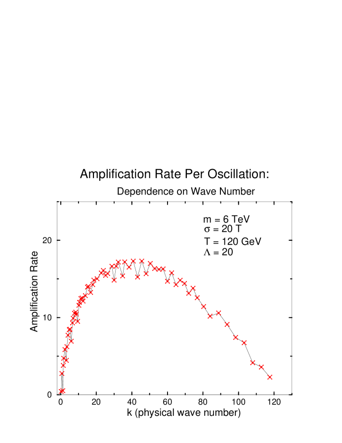
FIG. 2.: Amplification per cycle of EM fields, as a function of wave number.

FIG. 3.: Amplification per cycle of EM fields, as a function of temperature.

In Fig. 4 we represent the amplification rate per oscillation as a function of the amplitude of the scalar oscillations $\Lambda$. We show the range of variation with the conductivity $\sigma$ for range $\sigma=10-70T$. A notable feature of this picture are the dips for certain values of $\Lambda$ in both graphs. We believe that these are specific values, for which through the coupling of higher Fourier modes of the periodic function ${\it P}(\eta)$ in (62) to the scalar oscillation the leading exponential factor is canceled. But we do not have a clear understanding of this phenomenon.

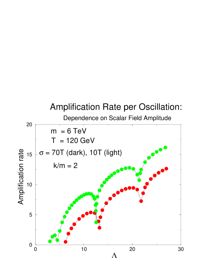
FIG. 4.: Amplification per cycle of EM fields, as a function of scalar field amplitude.

V CONCLUSIONS

A pseudoscalar field coupled to the hypercharge topological density can exponentially amplify HEM fields and develop a net Chern-Simons number in the symmetric phase of the EW plasma while it rolls or oscillates around the minimum of its potential. This mechanism could drastically change the electroweak scenario for baryogenesis and perhaps fix its two main dissabilities: the amount of asymmetry generated by electroweak processes and the character of the phase transition.

We have studied this mechanism for (pseudo)scalar masses in the TeV range, that could naturally appear if the scalar field is associated to supersymmetry breaking. In that case the coherent oscillations have to occur just before or during the phase transition in order to avoid the fast diffusion in the plasma of amplified magnetic modes once the scalar coherent motion terminates. In such a case the amplification spectrum is sharply peaked around the wave number $k_{\it max}\sim\frac{1}{2}\Lambda m$, total amplification is exponential in the number of cycles, and large amplification of magnetic modes, even $10^{12}$ or larger, can happen just after a few scalar oscillations depending on the particular values of the parameters of the model.

If the scalar field rolls instead of oscillating, the mechanism would be relevant for EW baryogenesis even if it takes place at higher temperatures before the phase transition. In this case, modes with wave number much smaller than the temperature of the plasma $k\ll T$ are maximally amplified. Once the scalar rolling terminates, the amplified magnetic modes remain frozen in the plasma and do not diffuse.

In a previous paper we have concluded that our mechanism would be able to generate enough asymmetry to explain the baryon number density to entropy ratio observed in the universe.

REFERENCES

- [1] A.D. Sakharov, JEPT Lett. 91B (1967) 24.
- [2] M.E. Shaposhnikov, JETP Lett. 44 (1986) 465; Nucl. Phys. B287 (1987) 757.
- [3] M.E. Carrington, Phys. Rev. D45 (1992) 2933; M. Dine R.G. Leigh, P. Huet, A. Linde and D. Linde, Phys. Lett. B283 (1992) 319; Phys. Rev. D46 (1992) 550; P. Arnold, Phys. Rev. D46 (1992) 2628; J.R. Espinosa, M. Quiros and F. Zwirner, Phys. Lett. B314 (1993) 206; W. Buchmuller, Z. Fodor, T. Helbig and D. Walliser, Ann. Phys. 234 (1994) 260; K. Kajantie, K. Rummukainen and M. Shaposhnikov, Nucl. Phys. B 407 (1993) 356; Z. Fodor, J. Hein, K. Jansen, A. Jaster and I. Montvay, Nucl. Phys. B 439 (1995) 147; K. Kajantie, M. Laine, K. Rummukainen and M. Shaposhnikov, Nucl. Phys. B 466 (1996) 189.
- [4] G.F. Giudice, Phys. Rev. D 45 (1992) 3177; S. Myint, Phys. Lett. B 287 (1992) 325; J. R. Espinosa, M. Quiros and F. Zwirner, Phys. Lett. B 307 (1993) 106; A. Brignole, J.R. Espinosa, M. Quiros and F. Zwirner, Phys. Lett. B 324 (1994) 181.
- [5] G.R. Farrar and M. Shaposhnikov, Phys. Rev. Lett. 70 (1993) 2833; 71 (1993) 210 (E); M.B. Gavela, P. Hernandez, J. Orloff, O. Pene and C. Quimbay, Mod. Phys. Lett. 9 (1994) 795; Nucl. Phys. B430 (1994) 382; P. Huet and E. Sather, Phys. Rev. D51 (1995) 379.
- [6] M. Giovannini and M.E. Shaposhnikov, Phys. Rev. D57 (1998) 2186; M. Giovannini and M.E. Shaposhnikov, Phys. Rev. Lett. 80 (1998) 22; M. Joyce and M.E. Shaposhnikov, Phys. Rev. Lett. 79 (1997) 1193; T. Vachaspati and G.B. Field, Phys. Rev. Lett. 73 (1994) 373.
- [7] E. Lifshitz and L.P. Pitaevskii, Statistical Physics, Part 2, Pergamonn Press, Oxford, 1981; A.L. Fetter and J.D. Walecka, Quantum Theory of Many Particle Systems, McGraw-Hill, New-York, 1971.
- [8] P. Elmfors, K. Enqvist and K. Kainulainen, hep-ph/9806403; K. Kajantie, M. Laine, J. Peisa, K. Rummukainen, M. Shaposhnikov, hep-lat/9809004.
- [9] R. Brustein and D.H. Oaknin, hep-ph/9809365.
- [10] M.S. Turner and L.M. Widrow, Phys. Rev. D37 (1988) 2743; W.D. Garretson, G.B. Field and S.M. Carroll, Phys. Rev. D46 (1992) 5346; J. Ahonen, K. Enqvist and G. Raffelt, Phys. Lett. B366 (1996) 224.
- [11] E.I. Guendelman and D.A.Owen, Phys. Lett. B276 (1992) 108.
- [12] D. Biskamp, Nonlinear Magnetohydrodynamics, Cambridge University Press, Cambridge, 1994; N.A. Krall and A.W. Trivelpiece, Priciples of Plasma Physics, San Francisco Press, San Francisco, 1986.
- [13] A.N. Redlich and L.C. Wijerwardhana Phys. Rev. Lett. 54 (1984) 970.
- [14] B. Campbell, S. Davidson, J. Ellis and K. Olive, Phys. Lett. B297 (1992) 118; L.E. Ibañez and F. Quevedo, Phys. Lett. B283 (1992); J.M. Cline, K. Kainulainen and K.A. Olive, Phys. Rev. Lett. 71 (1993) 2372; Phys. Rev. D49 (1994) 6394.
- [15] C.P. Dettmann, N.E. Frankel and V. Kowalenko, Phys. Rev. D48 (1993) 5655; R.M. Gailis, C.P. Dettmann, N.E. Frankel and V. Kowalenko, Phys. Rev. D50 (1993) 3847; A. Sil, N. Banerjee and S. Chatterjee, Phys. Rev. D53 (1995) 7369.
- [16] G. Baym and H. Heiselberg, Phys. Rev. D56 (1997) 5254; M. Joyce, T. Prokopec and N. Turok, Phys. Rev. D53 (1996) 2930; J.M. Cline and K. Kainulainen, Phys. Lett. B356 (1995) 19; J. Ahonen and K. Enqvist, Phys. Lett. B382 (1996) 40.
- [17] Y.B. Zeldovich, A.A. Rusmaikin and D.D. Sokoloff, Magnetic Fields in Astrophysics (Gordon and Breach, New York, 1983); E.N. Parker, Cosmical Magnetic Fields (Clarendon Press, Oxford, 1979).