The dissertation has been accomplished in 1993-1998 at the Institute of Theoretical Physics and Astronomy, Vilnius, Lithuania.

Institute of Theoretical Physics and Astronomy shares the joint doctoral degree-granting authority with Vilnius University, following the Resolution No 457 of the Government of Republic of Lithuania, April 14, 1998.

The Doctorate Committee

Chairman and scientific adviser:

• Egidijus NORVAIŠAS, Dr. (Institute of Theoretical Physics and Astronomy, Physical Sciences, Physics, 02P);

Members:

• Sigitas ALIŠAUSKAS, Dr. hab. (Institute of Theoretical Physics and Astronomy, Physical Sciences, Physics, 02P);

• Adolfas BOLOTINAS, Dr. hab., Prof. (Vilnius University, Physical Sciences, Physics, 02P);

• Kazimieras PYRAGAS, Dr. hab., Prof. (Vilnius Pedagogical University, Physical Sciences, Physics, 02P);

• Zenonas RUDZIKAS, Dr. hab., Prof. (Institute of Theoretical Physics and Astronomy, Physical Sciences, Physics, 02P);

Darbas atliktas 1993-1998 metais Teorinės fizikos ir astronomijos institute.

Doktorantūros ir daktaro mokslo laipsnio teikimo teisė Teorinės fizikos ir astronomijos institutui suteikta kartu su Vilniaus universitetu 1998 04 14 Lietuvos Respublikos Vyriausybės nutarimu Nr. 457.

Doktorantūros komitetas

Pirmininkas ir darbo vadovas

• Dr. Egidijus NORVAIŠAS (Teorinės fizikos ir astronomijos institutas, fiziniai mokslai, fizika, 02P);

Nariai:

• Habil. dr. Sigitas ALIŠAUSKAS (Teorinės fizikos ir astronomijos institutas, fiziniai mokslai, fizika, 02P);

• Prof. habil. dr. Adolfas BOLOTINAS (Vilniaus universitetas, fiziniai mokslai, fizika, 02P);

• Prof. habil. dr. Kazimieras PYRAGAS (Vilniaus pedagoginis universitetas, fiziniai mokslai, fizika, 02P);

• Prof. habil. dr. Zenonas RUDZIKAS (Teorinės fizikos ir astronomijos institutas, fiziniai mokslai, fizika, 02P);

Notations and conventions

• Bold letters indicate multiple quantity structure, which may vary from case to case. For example, $\boldsymbol{\alpha}$ denotes triple of Euler angles $(\alpha^{1},\alpha^{2},\alpha^{3})$, $\mathbf{r}$ denotes spatial vector $\vec{r}$ and $\mathbf{D}^{j}$ denotes Wigner matrix in representation $j$.

• Calligraphic letters $\mathscr{A},\mathscr{H},\mathscr{L},\mathscr{M}$ etc. denote densities.

• Appearance of carets (  $\hat{\mskip-3.0mu\mskip-3.0mu\mskip-3.0mu\mathscr{B}},\hat{V}^{a}_{t},\hat{}\mathbf{J}$, etc.) indicate an operator or its component. Note that we do not follow this convention for coordinate $\mathbf{q}$ (also sometimes for operators which are functions of $\mathbf{q}$ only) and momentum $\mathbf{p}$ operators in order to keep notations simpler.

• Special attention should be paid to $\hat{}\mathbf{J},\hat{}\mathbf{J}^{\prime}$ and $\mathbf{J},\mathbf{J}^{\prime}$ operators. Operators with hats $\hat{}\mathbf{J},\hat{}\mathbf{J}^{\prime}$ are dynamical operators (introduced in place of momentum operator $\mathbf{p}$ and depend on $\mathbf{q},\dot{}\mathbf{q}$), whereas operators without hats $\mathbf{J},\mathbf{J}^{\prime}$ are abstract SU(2) group generators. All group generators enter under $\operatorname{Tr}$ symbol, therefore, they yield representation dependence. Dynamical operators acting on appropriate states provide spin $\ell$ dependence.

• Dot over the symbol denotes full time derivative.

• The metric tensor $g^{\mu\nu}$ is $g^{00}=1,g^{0,i}=0,g^{i,j}=-\delta^{i,j}$ for spatial indices $i,j=1,2,3$. The four derivative $\partial^{\mu}=\frac{\partial}{\partial x_{\mu}}$ has components $(\partial/\partial t,-\nabla)$. The sign of totally anti-symmetric tensors (Levi-Cevita symbols) $\epsilon_{ijk},\quad\epsilon^{\mu\nu\sigma\gamma}$ are fixed by $\epsilon_{123}=-\epsilon^{123}=1,\quad\epsilon_{0123}=-\epsilon^{0123}=1$, respectively.

• Isovector of Pauli isospin matrices $\boldsymbol{\tau}$ in Cartesian coordinates have a form $\boldsymbol{\tau}_{1}=\bigl{(}\begin{smallmatrix}0&1\\ 1&0\end{smallmatrix}\bigl{)},\quad\boldsymbol{\tau}_{2}=\bigl{(}\begin{smallmatrix}0&-i\\ i&0\end{smallmatrix}\bigl{)},\quad\boldsymbol{\tau}_{3}=\bigl{(}\begin{smallmatrix}1&0\\ 0&-1\end{smallmatrix}\bigl{)}$.

• $*$ is a complex conjugation mark.

• SU(2), su(2) denotes the group and the group algebra, respectively.

• The indices $\alpha,\beta,\gamma\dotsc$ at the head of the Greek alphabet usually represent Euler angles. The middle Greek letters $\mu,\nu,\lambda,\rho,\eta,\dotsc$ represent axes in Minkowski space, whereas $i,j,k,l,o,p,r,s$ usually indicate spatial dimensions. Indices $a,b,c,d,e,f,g,h$ and $m,n$ are reserved for SU(2) values. Index $t$ denotes time component.

• The curly bracket $\bigl{\{}\ ,\ \bigr{\}}$ and the square bracket $\bigl{[}\ ,\ \bigr{]}$ denotes the anti-commutator and the commutator, respectively.

We assume summation convention under repeated (dummy) indices. Dummy indices sometimes can involve phase factors. In this case three indices are required for summation convention. For example, we assume summation in $(-1)^{a}A_{a}B^{(-a)}$, but not in $(-1)^{a}A_{a}$.

Natural units $c=\hbar=1$ are used in the work. Mass/energy, momentum then are usually measured in MeV (or fm^-1; $1$ MeV$=\frac{1}{197.3}\mathrm{fm}^{-1}$), length and time in MeV^-1. Unitary field $\mathbf{U}$ and model parameter $e$ are dimensionless, right $\mathbf{R}_{\mu}$ (left $\mathbf{L}_{\mu}$) Maurer-Cartan forms, Lagrange function, pion and sigma fields, pion decay constant $f_{\pi}$ have dimensions of MeV. Lagrange function density is proportional to MeV⁴. Vector, axial-vector and baryon current densities are proportional to MeV³, whereas Lagrange/Hamilton function density to MeV⁴.

Note

Notations in the first chapter differ from notations in the rest chapters, whereas notations are the same in second and third chapters.

List of publications

1. A. Acus, E. Norvaišas, and D. O. Riska, "Stability and Representation Dependence of the Quantum Skyrmion", Phys. Rev. C, V.57, Nr. 5, p.2597-2604 (1998)

2. A. Acus, E. Norvaišas, and D. O. Riska, "The Quantum Skyrmion in Representation of General Dimension", Nucl. Phys. A, V.614, p.361-372 (1997)

3. A. Acus and E. Norvaišas, "Stability of SU(2) Quantum Skyrmion and Static Properties of Nucleons", Lithuanian Journal of Physics, 1997, V.37, Nr. 5, p.446-448

4. E. Norvaišas and A. Acus, "Canonical quantization of SU(2) Skyrme model", Physical Applications and Mathematical Aspects of Geometry, Groups, and Algebras, Editors: H. D. Doebner, W. Scherer, P. Nattermann, World Scientific, Singapure, Vol.1, p.456-460, (1997)

5. A. Acus and E. Norvaišas, "New quantum corrections in Skyrme model for baryons," Proceedings of the International Workshop on Quantum Systems: new trends and methods, Editors: Y. S. Kim, L. D. Tomil’chik, I. D. Feranchuk, A. Z. Gazizov World Scientific, Singapure, p253-258, (1997)

6. A. Acus, "Barionu SU(2) Skyrme’o modelio tyrimas", Report to Lithuanian State Science and Studies Foundation, supervisor: dr E. Norvaišas, Nr.97-103/2F

Results of the investigation have been reported in the following conferences:

• "BARYONS ‘98", $\mathrm{8}^{\text{th}}$ International Conference on the Structure of Baryons, Bonn, September 22–26, 1998.

• 32${}^{\text{th}}$ Lithuanian National Conference of Physics, Vilnius, October 8–10, 1997.

• "XVII${}^{\text{th}}$ UK Institute for Theoretical High Energy Physicists", Durham, August 26–September 13, 1996.

• "XXI International Colloquium on Group Theoretical Methods in Physics", Goslar, July 15–20, 1996.

• "Origin of masses", International workshop, Tartu, June 19-22, 1996.

• "QS-96 Quantum Systems: New Trends and Methods", International workshop, Minsk, June 3-7, 1996.

• 31${}^{\text{th}}$ Lithuanian National Conference of Physics, Vilnius, February 5–7, 1996.

• "International Europhysics Conference on High Energy Physics", Brussels, July 27–August 2, 1995.

• "Nordic School in Particle Physics Phenomenology", Solvalla, June 11–17, 1994.

Preface

This thesis is a compendium of our work on extension of basic Skyrme model to arbitrary representations of SU(2) group, hoping that higher representations would be helpful for more adequate description of static baryon properties [1, 2, 3] .
General ideas and historical remarks. The idea that the ordinary proton and neutron might be solitons in nonlinear model has a long history. The first suggestion was made by T.H.R. Skyrme about 40 years ago [5]. The essential feature of the theory is the representation of the fundamental field quantities in terms of angular variables rather than linear ones. Realistic three-dimensional model is possible only when there are also three angular variables. The condition is satisfied by the pion fields of nature. The periodicity of angular variables introduces a new constant of motion, which measures the number of times that space (three dimensions) is mapped by the fields onto the elementary volume of angular space and which can be interpreted as a baryon number. The origin of the new constant of motion is related to topological features of the Skyrme model. In contrast, conservation of energy and momentum follows from space-time symmetry, as usually.

The mathematical construction outlined above is to ensure possibility of particle-like states "of a kind that cannot be reached by perturbation theory and which cannot necessarily be discounted by general arguments" [6]. To provide readers a link between fundamental theory of strong interactions (QCD) and Skyrme model we need to consider briefly the chiral symmetry concept and, therefore, the idea of isospin.

The concept of isospin was introduced in 1933 by W. Heisenberg, who considered proton and neutron as different projections of single state. From contemporary point of view W. Heisenberg actually assumed SU(2) (flavour) symmetry of nuclear interactions. In 1962 M. Gell-Mann succeeded much more in suggesting very predictive SU(3) (flavour) symmetry of strong interactions (The Eightfold Way) and the concept of isospin was extended to all baryons. The SU(3) symmetry had enormous influence in becoming of QCD: it was realized that each basis element, i.e. a product of quark and anti-quark functions, can be identified with some hadron state. The entire basis, therefore, is interpreted as multiplet of hadrons, belonging to irreducible representation of (flavour) SU(3) group.

A revival of interest in the Skyrme model [5, 6], begins from the work [8] of G.S. Adkins et al., who demonstrated that this model could fit observed properties of the baryons to an accuracy of about 30%. This rebirth of attention was stimulated by the belief that some such model is the long-wavelength limit of QCD, as reviewed, e.g., in Refs. [9, 10]. The interplay between various phenomenological models and QCD is still open problem [11].
Extensions and modifications of basic Skyrme model. In the intervening period, there has been a large number of works extending the range of applications, modifying and extending the model, and improving the way in which consequences are drawn from it. This work also serves as an extension of basic Skyrme model to arbitrary SU(2) representation. Among the further applications, the most prominent have been to pion-nucleon scattering [12, 13] and the two-nucleon problem [14, 15], and, very recently, to multi-soliton "chemistry" [16, 17, 18]. The basic Skyrme model has been extended in various directions. Excluding the mention of models that contain the quarks explicitly, one encounters in the literature models with higher-order terms involving the same fields [19, 20] or even higher unitary groups [21], models in curved space [22, 23] and models in which vector mesons have been added [24, 25, 26], as well as extensions to include strange [27] and even charmed mesons [28]. Related but more fundamental extension of the basic Skyrme model is the incorporation of the Wess-Zumino term into this theory. This term eliminates an extra discrete symmetry that is not a symmetry of QCD [29] and, therefore, has far reaching consequences and, of course, no lack of attention [30].

All these models are first presented as classical field theories, since one can do much physics using only selected classical solutions. The need to address the problem of quantization is, however, manifested in the intrinsic properties of the classical solution.

The capability of extracting interesting physics from the Skyrme model is grounded on the existence of a special solution of the classical field theory, the hedgehog skyrmion. Like all interesting classical (or mean field) solutions it breaks some of the symmetries of the underlying Lagrangian. The hedgehog skyrmion violates translation, spatial rotation, and iso-spatial rotation symmetry. The restoration of these symmetries requires, at the very least, the quantization of the generators of the symmetry transformations and of the associated canonically conjugate collective coordinates. As a consequence, maximum attention has been paid to this aspect of the problem of quantization [31]. In addition, to study pion-baryon scattering [12, 32, 33], it is necessary to discuss quantization of the small oscillations of the pion field [34] (for different approach see [35]). There have also been some discussion on quantization of radial oscillations [36, 37, 38] in connection with problems of stability. Other quantization methods applied to Skyrme model include cutoff quantization [39], (which uses short-distance cutoff $\epsilon:\quad F(\epsilon)=\pi$), the general covariant Hamiltonian method [40, 41, 42] (which preserves the original symmetry of classical Lagrangian), Kerman-Klein quantization procedure [43] (based on formal quantization of entire classical field). Due to rich and beautiful mathematical structure the model has numerous applications.
Applications of Skyrme model. Despite the original model has been introduced to describe strongly interacting particles, there are attempts to apply similar gauged construction to describe weak interactions ("electroweak skyrmions") [44] (p.250). Apart from high energy physics the model proved to be useful in cosmology [45] and solid state physics [46, 47]. Before brief review of the manuscript organization we explicitly state main tasks this thesis is intended to solve.
Main tasks:

1. Investigate representation dependence of the quantization procedure [48] applied to the SU(2) Skyrme model.

2. Numerically evaluate obtained expressions for physical quantities and compare the results with experimental data.

Scientific novelty. This work demonstrates the new possibilities to extend basic Skyrme model to arbitrary representations. Quantization of the Skyrme model (in collective coordinate approach from the outset) yields different quantum Lagrangian density for each SU(2) group representation $j$. The classical limit of these quantum Lagrangian densities is the same original Skyrme Lagrangian density. For the first time it has been shown that stable quantum solitons exist both for spin, isospin $\ell=\frac{1}{2}$ and $\ell=\frac{3}{2}$ states. These quantum solitons possesses Yukawa asymptotic and, therefore, imply non-vanishing pion mass. Noether currents, magnetic momenta etc., operators have been calculated and numerically evaluated in this approach for self-consistent quantum chiral angles in various representations $j$.

The generalization considered in the work has far-reaching consequences and, we believe, can readily be extended to other models and theories.
Manuscript organization. The manuscript is organized into three chapters plus appendices, containing numerous tables and illustrations. Chapters and sections (if structure of the latter is complicated enough) have short information about its content and, therefore, not need to be repeated here. We find useful, however, briefly to describe what purposes each chapter is intended to serve. Chapter I contains mathematical formulation and physical motivation of the Skyrme model in background level. Apart from few presentation details it contains no new results. We give formulation of classical Skyrme model in group theory terms and introduce mathematical apparatus which is convenient for model formulation in arbitrary representation in Chapter II. This chapter includes results of Ref. [49]. Chapter III contains main new results and deals with the quantization of the Skyrme model.

Despite the thesis has no lack of references when investigating concrete problems we found useful to provide a list of sources about the entire model. These are books [44, 50] and review articles [51, 52, 53]. Literature on solitons currently is untraceable, but we still mention few books, namely [4, 54, 55] to begin with.
Acknowledgments

• First of all I am indebted to my teacher and collaborator Egidijus NORVAIŠAS. It has been a joy and privilege these five years to have benefited from his gently guidance, clear ideas and informal communication.

• I tender thanks to my wife Janina and our sons Algirdas and Kestutis for everything, most of all keeping me sane and making me happy through it all.

• I also would like to thank my doctorate committee for consultations and support, many teachers both at the University and school, as their help and education have played an important role in my further investigations.

• Many thanks to Vytautas ŠIMONIS and Rimantas ŠADŽIUS for careful reading of the manuscript, also Tadas KRUPOVNICKAS in helping me with illustrations.

• I am grateful to the administration of Institute of Theoretical Physics and Astronomy for taking care of our (constantly improving) work conditions.

• Many thanks to staff of library of Institute of Theoretical Physics and Astronomy for quick and comprehensive service.

• I am indebted to Gediminas VILUTIS, Vygandas LAUGALYS, Gintaras VALIAUGA, Gytis VEKTARIS, Gintautas GRIGELIONIS, Edvardas DU-KO, Artūras KULIEŠAS for help and guidance in sideless jungle of enormous (and still very rapidly expanding) Computerland.

• Finally I would like to thank many others at Institute of Theoretical Physics and Astronomy, and especially our coffee team (Gediminas JUZELIŪNAS, Bronislovas KAULAKYS, $\dots$) for inspiration, companionship and support.

• This study was supported by Lithuanian Government, Lithuanian State Science and Studies Foundation, by Grant N LA5000 from the International Science Foundation (in part), and by Joint grant N LHU100 from Lithuanian Government and ISF (in part).

Chapter I Introduction to the Skyrme model

This chapter is intended to provide very short but more or less consistent introduction to the Skyrme model. From this point of view it is essential to clear out difference between models realized linearly and nonlinearly. The simplest examples are linear and nonlinear $\sigma$ models. Skyrme model then arises naturally by adding the fourth-order term in field functions to nonlinear $\sigma$ model Lagrangian. This term enables existence of stable soliton in three spatial dimensions (skyrmion) and, therefore, is called a stabilizing term.

I.1. Linear $\sigma$ model in two spatial dimensions

We start with linear $\sigma$ model. When physical boundary conditions are imposed, all model solutions fall into disconnected classes regardless of what equations of motion are. It is this property which is peculiar to nonlinear models only and play an important role in the Skyrme model particularly.

I.1.1. The Lagrangian

Let’s take $\boldsymbol{\Phi}$ to be a scalar doublet of real fields $(\Phi_{1},\Phi_{2})$ and consider the Lagrangian

$$\mathscr{L}=-\frac{1}{2}\partial_{\mu}\Phi_{r}\partial^{\mu}\Phi_{r}-(\left|\boldsymbol{\Phi}\right|^{2}-a^{2})^{2};\qquad r=1,2;\quad a^{2}>0.$$ (I.I.1.1)

Here we understand $\left|\boldsymbol{\Phi}\right|^{2}=\Phi_{r}\Phi_{r}$ and $\mu=0,1,2$ ($0$ denotes time component). Assume that for $\mathbf{x}\rightarrow\infty$ field configuration tends to some constant state

$$\Phi_{1}^{2}+\Phi_{2}^{2}\rightarrow a^{2},\qquad\text{for}\left|\mathbf{x}\right|\rightarrow\infty$$ (I.I.1.2)

with approach rate, which guarantees finiteness of total system energy $E$. Then the set $\boldsymbol{\Phi}_{\infty}=\left(\Phi_{\infty 1},\Phi_{\infty 2}\right)$ of all fields at spatial infinity make up a circle $S^{1}$. Spatial infinity in argument plane also can be imaged as a circle $\tilde{S}^{1}$, with infinitely large radius

$$x^{2}_{1}+x^{2}_{2}=R^{2},\qquad R\rightarrow\infty.$$ (I.I.1.3)

Field $\boldsymbol{\Phi}_{\infty}$ maps a circle $\tilde{S}^{1}$ to a circle $S^{1},\quad\boldsymbol{\Phi}_{\infty}:\quad\tilde{S}^{1}\rightarrow S^{1}.$ Identification of infinities with a circle of infinite radius does not involve any topology change. The hint is similar to coordinate system change. We have here spaces — both argument and function space — flat. Moreover, these spaces are vector spaces as well. Consider first a vacuum (or trivial) solution $\boldsymbol{\Phi}_{\rm vac}(x_{1},x_{2})\equiv(a,0)$. At spatial infinity the field $(\boldsymbol{\Phi}_{\infty})_{\rm vac}=\lim\limits_{R\rightarrow\infty}\boldsymbol{\Phi}_{\rm vac}$ maps all points of $\tilde{S}^{1}$ circle (argument infinity) to the same vacuum point $(a,0)$ of function space $S^{1}$. Thus $(\boldsymbol{\Phi}_{\infty})_{\rm vac}$ is characterized by zero winding number: $(\boldsymbol{\Phi}_{\infty})_{\rm vac}\in Q^{\infty}_{0}$. To $(\boldsymbol{\Phi}_{\infty})_{\rm vac}$ we can, therefore, associate all maps $\boldsymbol{\Phi}^{(0)}_{\infty}$ which are homotopic to $(\boldsymbol{\Phi}_{\infty})_{\rm vac}$. The set of all maps $\boldsymbol{\Phi}^{(0)}_{\infty}$ makes up the trivial sector $Q_{0}^{\infty}$ of system configuration space $Q^{\infty}$ (see Fig. I.1).

Figure I.1. Example of zero winding number maps.

Of course, one can choose any other vacuum state simply redefining $\boldsymbol{\Phi}_{\rm vac}(\mathbf{x})=(a/\sqrt{2},a/\sqrt{2})$ or more generally $\boldsymbol{\Phi}_{\rm vac}(x_{1},x_{2})=(a\cos\chi,a\sin\chi)$, where $\chi$ is fixed from $[0,2\pi]$ (see Fig. I.1 $\mskip-3.0mu{}_{c}$). All vacuuma belong to trivial $n=0$ sector and are homotopic to $\boldsymbol{\Phi}_{\rm vac}=(a,0)$. The homotopy can be defined as $h_{2}(t)=(a\cos t\chi,a\sin t\chi)\quad t\in[0,1]$ (see Fig. I.1 $\mskip-3.0mu{}_{b,c}$). One could think about gauge freedom corresponding to transformation from one vacuum to another. With any vacuum choice model SO(2) symmetry becomes spontaneously broken. Physical motivation comes from tunnelling possibility: vacuuma aren’t separated by any potential barrier, therefore, in the case of such vacuuma interference fields must rotate everywhere in space. This involves infinite rotational energy [44] (p.107). Of course such interference also restores SO(2) symmetry of the ground state and, therefore, should be forbidden.

I.1.2. Soliton sectors and invariants of linear $\sigma$ model

A field $\boldsymbol{\Phi}_{\infty}^{(1)}(\theta)$ of the sector $Q^{\infty}_{1}$ can be defined as $\boldsymbol{\Phi}_{\infty}^{(1)}(\theta)=(a\cos\theta,a\sin\theta)$. When $\theta$ runs from $0$ to $2\pi$ all points on $S^{1}$ are covered once and only once. $\boldsymbol{\Phi}_{\infty}^{1}$ is a typical winding number one map (see Fig. I.2). The equivalence class of maps homotopic to $\boldsymbol{\Phi}^{(1)}_{\infty}$ forms the winding number one sector $Q^{\infty}_{1}$. The winding number $n$ map can be defined as $\boldsymbol{\Phi}_{\infty}^{(n)}(\theta)=(a\cos n\theta,a\sin n\theta)$, where $n$ is an integer, due to our requirement of $\boldsymbol{\Phi}$ single valuedness on $\tilde{S}^{1}:\quad\boldsymbol{\Phi}_{\infty}^{(n)}(0)=\boldsymbol{\Phi}_{\infty}^{(n)}(2\pi)$. $Q^{(\infty)}_{n}$ consists of all $\boldsymbol{\Phi}^{(n)}_{\infty}$ homotopic maps. We remind that $\Phi^{(n)}_{\infty}$ with any $n$ (not only $n=0$) satisfy (I.I.1.2). From this picture it becomes clear that it is not possible to deform a field $\boldsymbol{\Phi}^{(n)}_{\infty}$ to a field $\boldsymbol{\Phi}^{(m)}_{\infty}$ continuously, if $n\neq m$. Indeed, for the action we need to cut the mapping curve and take off $|n-m|$ twists. Thus the fields in sector $Q_{n}^{(\infty)}$ are not homotopic to fields in $Q_{m}^{(\infty)}$ for $n\neq m$. As a consequence, system configuration space $Q^{\infty}$ falls into an infinite number of disconnected components $Q^{\infty}_{n}=\{\boldsymbol{\Phi}^{(n)}_{\infty}\}$, $Q^{\infty}$ being a union $\operatorname{\cup}\limits_{n}Q^{\infty}_{n}$. The same is then true for the space $Q$ of fields defined over all space: $Q=\operatorname{\cup}\limits_{n}Q_{n}$. Here $Q_{n}$ is the space of all configurations $\boldsymbol{\Phi}^{(n)}$ whose limit as $|\mathbf{x}|\rightarrow\infty$ is an element $\boldsymbol{\Phi}_{\infty}^{(n)}$ of $Q_{n}^{(\infty)}$. For example, $\boldsymbol{\Phi}^{(n)}$ at given time $t_{0}$ can be defined by

$$\boldsymbol{\Phi}^{(n)}(\mathbf{x},t_{0})=f(|\mathbf{x}|)\,\boldsymbol{\Phi}_{\infty}^{(n)}\Bigl{(}\frac{\mathbf{x}}{|\mathbf{x}|}\Bigr{)},$$ (I.I.1.4)

where $f(|\mathbf{x}|)$ is any smooth function, such that $f(\infty)=1,\quad f(0)=0$.

The physical significance of the integer $n$ associated with the field $\boldsymbol{\Phi}^{(n)}(\mathbf{x},t)$ is that it is an integral of motion. The integer is just the label of homotopy classes of the fields at a fixed time. Sectors $Q_{n}\quad(n\neq 0)$ are topologically stable in the sense that a field in $Q_{n}$ will not evolve in time to the vacuum (an element of $Q_{0}$) or to a field in any other sector $Q_{m}\quad(m\neq n)$, since evolution in time is a continuous deformation.

The existence of inequivalent topological sectors leads to additional invariants in the theory. These new invariants of quite different origin is the most interesting and important point in such models. As a consequence, we have two kinds of invariants:

• Invariants which are closely related to the symmetry of the system, under simultaneous coordinate frame and fields change (corresponding to this frame transformations). We can find all these invariants by Noether theorem. Examples of the invariants are: energy, momentum, angular momentum, electromagnetic charge.

• Invariants, involving boundary conditions in one or another way. Conservation of the number of particles in classical mechanics (in conservative systems) is an example.

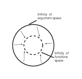
Figure I.2. Example of winding number one map in linear $\sigma$ model.

Let us concentrate on the second type of invariants. It has been shown that solutions from one sector cannot evolve in time to the solutions of any other sector. Consequently, we need discrete quantity to label each sector. The most natural choice seems to be the number of twists, describing mapping of one circle onto another. The number is called a topological charge. One could introduce a conserved topological current density, corresponding to the charge

$$J^{\rm top}_{\mu}\sim\epsilon_{\mu\sigma\rho}\epsilon^{rs}\partial^{\sigma}\Phi^{r}\partial^{\rho}\Phi^{s}\quad\mu,\sigma,\rho=0,1,2;\quad r,s=1,2.$$ (I.I.1.5)

It is easy to check that expression (I.I.1.5) has a divergence zero and meets our requirements. We stress that the current density is conserved irrespective of what the equations of motion are (because of the antisymmetric properties of $\epsilon_{\mu\sigma\rho}$) and thus it is topological. The corresponding charge density is

$$J^{\mathrm{top}}_{0}={\rm div}\mathbf{P},\qquad\text{where}\qquad P_{k}\sim\epsilon_{kl}\epsilon^{rs}\Phi^{r}\partial_{l}\Phi^{s};\quad k,l=1,2.$$ (I.I.1.6)

The charge $Q^{\mathrm{top}}\sim\int J^{\mathrm{top}}_{0}\mathrm{d}^{2}\mathbf{x}$ is nonzero only for fields $\boldsymbol{\Phi}$ with non-vanishing asymptotic [56], which is realized, for example, by the Higgs mechanism.

I.1.3. Derrick theorem

The existence of topologically stable sectors and conservation of topological current are independent on the Lagrangian form and, thus, on equations of motion. The presence of such sectors, therefore, does not guarantee that equations of motion actually have solutions in each sector. It is known that Lagrangian (I.I.1.1) does not lead to nontrivial stable static solutions of equations of motion if only the spatial dimension is $D\neq 1$. This can be shown by simple scaling argument of Derrick [44, 57]. Suppose that $\boldsymbol{\Phi}_{\rm cl}$ is static solution and the energy of the solution consists of terms $E=E_{1}+E_{2}$:

$$E_{1}=\frac{1}{2}\int\mathrm{d}^{D}\mathbf{x}(\partial_{i}(\boldsymbol{\Phi}_{\rm cl})_{s})^{2}\quad\text{and}\quad E_{2}=\int\mathrm{d}^{D}\mathbf{x}U[((\boldsymbol{\Phi}_{\rm cl})_{s})^{2}]\quad i=1,2,\dotsc,D.$$ (I.I.1.7)

Under a scaling transformation $\boldsymbol{\Phi}_{\rm cl}(\mathbf{x},t)\rightarrow\Phi_{\rm cl}(\lambda\mathbf{x},t)$ these terms scale as

$$E\equiv E(1)\rightarrow E(\lambda)=\lambda^{2-D}E_{1}+\lambda^{-D}E_{2}.$$ (I.I.1.8)

Requiring that $\lambda=1$ corresponds to energy $E$ minimum yields the condition

$$\frac{\mathrm{d}E(\lambda)}{\mathrm{d}\lambda}\Bigl{|}_{\lambda=1}=0\quad\text{or}\quad(2-D)\,E_{1}=D\,E_{2}.$$ (I.I.1.9)

Since $E_{1},E_{2}\geq 0$, it follows that $E_{1}=E_{2}=0$ when $D>2$. This implies that $\boldsymbol{\Phi}_{\rm cl}$ must be the vacuum solution for $D>2$. In the case $D=2$, we have $E_{2}=0$, so that $((\Phi_{\rm cl})_{1})^{2}+((\Phi_{\rm cl})_{2})^{2}=a^{2}$ for all $\mathbf{x}$. This requires that $\boldsymbol{\Phi}_{\rm cl}$ (as $|\mathbf{x}|\rightarrow\infty$) has zero winding number and hence is in $Q_{0}^{(\infty)}$. We can prove this result as follows. Let $r,\theta$ denote polar coordinates in the plane. For any nonzero $r$, $\boldsymbol{\Phi}_{\rm cl}$ defines a map of the circle (with coordinate $\theta$) to a circle (because of the condition $((\Phi_{\rm cl})_{1})^{2}+((\Phi_{\rm cl})_{2})^{2}=a^{2}$). The winding number $n$ of this map cannot depend on $r$, as changing $r$ is a continuous change. When $r\rightarrow 0$, all values of $\theta$ represent the same spatial point, so that $n\rightarrow 0$. Hence n is identically zero which proves the result.

I.2. Simplest nonlinear topological model

The simplest model which modifies space topology can be found in one-dimensio-nal field theory. Consider the set of all mappings $\alpha$ from the real line $R^{1}$ (argument space) onto the circle $S^{1}$ (function space). $S^{1}$ can be parametrized by two real variables $\boldsymbol{\Phi}=(\Phi_{1},\Phi_{2})$, whose squares add up to one: $\Phi_{1}^{2}+\Phi_{2}^{2}=1$. Note that function space is not flat (circle $S^{1}$). To prevent the escape of interesting structures at infinity we consider only the class of functions on $S^{1}$, such that $\boldsymbol{\Phi}(\infty)=\boldsymbol{\Phi}(-\infty)$. The restriction of functions class allows us to identify argument space (line $R^{1}$) with a circle. In other words it makes possible compactification of $R^{1}$ to a circle. A field $\boldsymbol{\Phi}^{(1)}$ from $n=1$ sector may be illustrated pictorially by a strip familiar with Möbius strip, except that the Möbius strip has a twist through $\pi$ whereas the sector $n=1$ field has a twist through $2\pi$. $\boldsymbol{\Phi}^{(1)}(x)$ then specifies twist angle of the strip about its center line at a given point $x$. Note quite different meaning we give to the external circle in this (see Fig. I.3) and linear case (Fig. I.2_b). Since by classical field we mean a field that is single-valued under the action of the rotation group, it follows that particles involved must be bosons. Quantization of such a classical field introduces a quantity that can be interpreted as a particle number. It is known that after quantization the states, corresponding to $n=1$ classical configuration, are, in fact, fermion states. Dynamics and quantum mechanical operators can be introduced into this theory [5, 59].

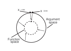
Figure I.3. Example of one-dimensional model map in a simple nonlinear model.

To summarize, the simple nonlinear model fields are subject to nonlinear constraint, when linear $\sigma$ model fields are not. This explains the need to reduce one argument space dimension in order to have the same global symmetry group for both models. In other words, function space of the first model is a flat space (vector space as well), when function space of the second one is a compact manifold (not a vector space at all).

I.3. Nonlinear $\sigma$ model in two spatial dimensions

In this section we formulate nonlinear $\sigma$ model in fundamental SU(2) representation using well known Pauli and rotation matrices technique. The Skyrme model then is obtained by adding forth order term in field functions which ensures stable soliton solution in 3D. As a consequence, Skyrme model inherits all essential features from nonlinear $\sigma$ model.

I.3.1. Formulation

It was sufficient to look at $Q^{\infty}$ (the space of physical fields at spatial infinity) for the topological consideration in the linear $\sigma$ model. For solitons in nonlinear models it is often necessary to consider the topology of physical fields defined over all space. Physical fields in these models for all points $\mathbf{x}$ take values in a manifold M which generally is not a vector space.

By definition group G acts on manifold M transitively, if for any pair $p,p^{\prime}\in\text{{\goth M}}$ there exists an element $g\in\text{{\goth G}}$, such that $T_{g}(p)=p^{\prime}$. Assume, this is the case. Then M is called a homogeneous space for G. If $\text{{\goth g}}_{p}$ is the stability group of point $p\in\text{{\goth M}}$:

$$\text{{\goth g}}_{p}=\{h\in\text{{\goth G}}|hp=p\},$$ (I.I.3.1)

and M is a homogeneous space for G  then any two $\text{{\goth g}}_{p},\text{{\goth g}}_{p^{\prime}}\quad p,p^{\prime}\in\text{{\goth M}}$ are isomorphic. If $p\neq p^{\prime}$ and $T_{g}(p)=p^{\prime}$ the isomorphism $\text{{\goth g}}_{p}\rightarrow\text{{\goth g}}_{p^{\prime}}$ can be defined: $h\mapsto ghg^{-1}$. Now we can identify M with space of left cosets G$/$g by the following procedure. First let’s fix point $p_{0}\in\text{{\goth M}}$. With each class of left cosets $\{g\text{{\goth g}}\}$ we identify point $T_{g}(p_{0})$, where $\text{{\goth g}}=\text{{\goth g}}_{p_{0}}$ is a stability group of point $p_{0}\in\text{{\goth M}}$. The identification is in one-to-one correspondence and do not depend on particular $g$ in the class of left cosets.

The nonlinear $\sigma$ model in two spatial dimensions has G $=$SU(2)$,\quad$ g $=$U(1) $\equiv\{{\mathrm{e}}^{i\alpha{J_{z}}},0\leq\alpha\leq 2\pi\}$ and M$=$G$/$g  is a two sphere $S^{2}$. To show this, define

$$K\equiv gJ_{z}g^{\dagger}=n_{a^{\prime}}J_{a^{\prime}},\quad a^{\prime}=(x,y,z)\equiv(1,2,3),$$ (I.I.3.2)

where $g\in\mathrm{SU(2)}$ and $J_{a^{\prime}}$ are generators of SU(2).

$K$ is an invariant under transformation $\pi:g\rightarrow g\mathrm{e}^{i\alpha J_{z}}$. A map $\pi$ projects $g\mathrm{e}^{i\alpha J_{z}}\in\text{{\goth G}}$ for all $\alpha$ to the same point of left cosets $\{g\text{{\goth g}}\}$. Since $\alpha$ is a continuous parameter, $\{g\text{{\goth g}}\}$ defines a two dimensional manifold, namely a two sphere $\mathrm{SU(2)/U(1)}=S^{2}$. Indeed, the scalar product of $n_{a^{\prime}}$ is $1$,

$$\operatorname{Tr}K^{2}=n_{a^{\prime}}n_{a^{\prime}}\equiv(n_{a^{\prime}})^{2}=1.$$ (I.I.3.3)

Fields $\Phi_{a^{\prime}}(x_{1},x_{2},t)$ of nonlinear 2-dimensional $\sigma$ model are subjects to the constraint: $\Phi_{a^{\prime}}(\mathbf{x},t)\Phi_{a^{\prime}}(\mathbf{x},t)=1$ and thus can be identified with $n_{a^{\prime}}$. The action of G on these fields yields

$$\Phi^{\prime}_{a^{\prime}}=R_{a^{\prime}b^{\prime}}(g)\Phi_{b^{\prime}},$$ (I.I.3.4)

where $R_{a^{\prime}b^{\prime}}$ is the usual rotation matrix — an element of adjoint representation of SU(2): $\mathbf{R}\in SO(3)$. Note that the constraint is invariant under this action of G.

The Lagrangian density is chosen so that it is invariant under G.

$$\mathscr{L}=-\frac{\beta}{2}\partial_{\mu}\Phi_{a^{\prime}}\partial^{\mu}\Phi_{a^{\prime}},\quad\beta=\mathrm{const},\quad\mu=0,1,2.$$ (I.I.3.5)

Because of the constraint on $\boldsymbol{\Phi}_{a^{\prime}}$, the Lagrangian (I.I.3.5) does not describe a free system. Interactions of the field with itself are implicit. To see this, one can write $\mathscr{L}$ in terms of two independent degrees of freedom, say $\Phi_{1}\equiv\Phi_{x}$ and $\Phi_{2}\equiv\Phi_{y}$

$$\mathscr{L}=-\frac{\beta}{2}\left(\frac{2-\Phi_{k}\Phi_{k}}{1-\Phi_{k}\Phi_{k}}\right)(\partial_{\mu}\Phi_{k})^{2},\quad\Phi_{3}\neq 0,\quad k\ \text{is summed over\ }1\text{\ and\ }2.$$ (I.I.3.6)

Note that the action of G is nonlinear in terms of two degrees of freedom.

The energy density associated with (I.I.3.5) is

$$\mathscr{E}(\mathbf{x},t)=\frac{\beta}{2}\bigl{(}(\partial_{0}\Phi_{a^{\prime}})^{2}+(\partial_{i}\Phi_{a^{\prime}})^{2}\bigr{)};\quad i=1,2.$$ (I.I.3.7)

I.3.2. Topological structure

The vacuum solution (which is subject to the constraint on $\boldsymbol{\Phi}$) is $\boldsymbol{\Phi}_{\mathrm{vac}}=\mathrm{const}$. $\mathscr{E}$ is invariant under global SU(2) transformations. Thus $\boldsymbol{\Phi}_{\mathrm{vac}}$ can be reduced to $(0,0,1)$ by action of SU(2) without affecting the energy ($\mathscr{E}\equiv 0\quad\text{for}\quad\boldsymbol{\Phi}_{\mathrm{vac}}$). After the choice only rotations about the third axis leave the vacuum invariant, consequently, the global SU(2) is spontaneously broken to a global U(1), by special vacuum choice.

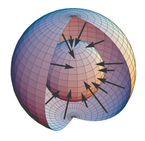
Figure I.4. Example of mappings: $\tilde{S}^{2}$ sphere $\rightarrow$ $S^{2}$ sphere.

Next, consider general configuration with nonzero, but finite energy. Let us first show that homotopic sector generation mechanism described in linear $\sigma$ model in Sec. I.1 now fails. Indeed, for large $|\mathbf{x}|\equiv R$ the fields $\boldsymbol{\Phi}$ define a mapping from circle $S^{1}$ with radius $R$ to $S^{2}$. Since $\pi_{1}(S^{2})=0$ this mapping is homotopic to $\boldsymbol{\Phi}_{\mathrm{vac}}$ at $|\mathbf{x}|=R$. Despite the fail there is a way out. Indeed, finiteness of energy requires $\boldsymbol{\Phi}(\mathbf{x},t)$ to approach $\boldsymbol{\Phi}_{\mathrm{vac}}$ as $r\rightarrow\infty$ and that the rate of approach is fast enough to guarantee that the energy $E$ is finite. Again we choose $\boldsymbol{\Phi}_{\mathrm{vac}}=(0,0,1)$. Assume that $\boldsymbol{\Phi}$ approaches $\boldsymbol{\Phi}_{\mathrm{vac}}$ and there is no angle dependent limit at $r=\infty$. Thus, we may think of all points at spatial infinity as being a single point. Such a restriction of function class $\boldsymbol{\Phi}$ essentially converts (in topological but not metrical sense) the plane $R^{2}\equiv\{(x_{1},x_{2})\}$ at a constant time $t_{0}$ to the surface of a two sphere $\tilde{S}^{2}$. The fields $\boldsymbol{\Phi}=(\Phi_{1},\Phi_{2},\Phi_{3})$ are well defined on this $\tilde{S}^{2}$ in view of boundary conditions. Consider this in detail. Let $\xi_{a},\quad a=1,2,3$ be the stereographic coordinates associated with $\mathbf{x}$

$$\xi_{a}(\mathbf{x})=\frac{2x_{a}}{r^{2}+1},\quad a=1,2;\quad\xi_{3}(\mathbf{x})=\frac{r^{2}-1}{r^{2}+1}$$

$$\xi_{1}^{2}(\mathbf{x})+\xi_{2}^{2}(\mathbf{x})+\xi_{3}^{2}(\mathbf{x})=1,\quad r^{2}=x_{a}x_{a}.$$ (I.I.3.8)

Coordinates $\boldsymbol{\xi}$ span a two-sphere $\tilde{S}^{2}$. They are not global valid coordinates for $R^{2}$ which unlike $S^{2}$ is not a compact manifold. Indeed, all the "points of infinity" of $R^{2}$ which correspond to $r\rightarrow\infty$ are mapped to one point of $S^{2}$, namely $(0,0,1)$. In reality the "points of infinity" are not points at $R^{2}$ at all. Thus, to get a topologically accurate representation of $R^{2}$ we should remove the north pole $(0,0,1)$ from $\tilde{S}^{2}:\quad R^{2}=\tilde{S}^{2}\backslash\{(0,0,1)\}$.

The topological difference between $R^{2}$ and $S^{2}$ can make difference for some functions. For example, the function $f(\mathbf{x})=|\mathbf{x}|$ is a continuous function on $R^{2}$, but the function obtained by the substitution $x_{a}=\xi_{a}/(1-\xi_{3})$ is not a continuous function on $\tilde{S}^{2}$, becoming infinite at north pole $\xi_{3}=1$. Another example is the function $\bar{}\mathbf{x}=\mathbf{x}/|\mathbf{x}|$ which is continuous on $R^{2}$, while its image function on $\tilde{S}^{2}$ has no well defined limit as the north pole is approached. However, for functions which approach a constant limit as $r\rightarrow\infty$, the change of variable $\mathbf{x}\rightarrow\boldsymbol{\xi}$ does produce a well defined function on $\tilde{S}^{2}$. In this sense then, because of the boundary condition on $\boldsymbol{\Phi}$, we can imagine that the space on which the field $\boldsymbol{\Phi}$ is defined is $\tilde{S}^{2}$.

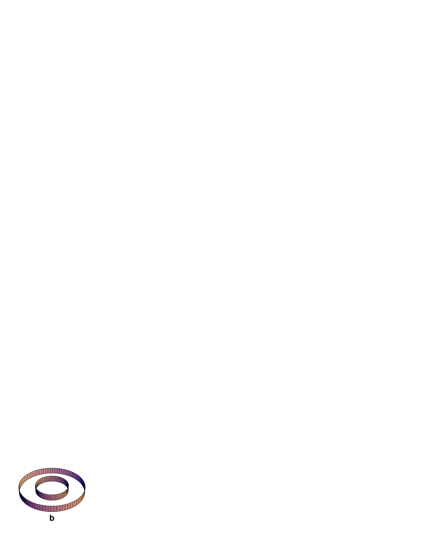
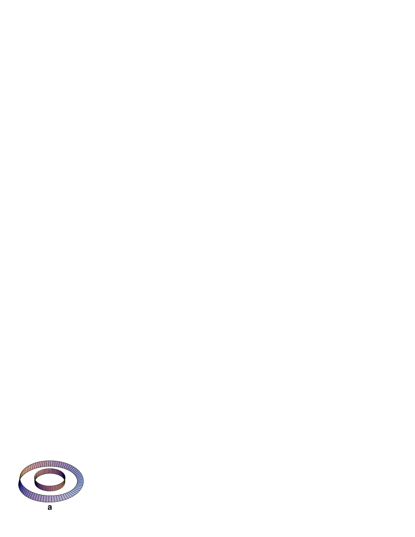
Figure I.5. Examples of mappings: cylinder $\rightarrow$ cylinder and cylinder $\rightarrow$ Möbius strip.

Thus, the configuration space $Q$ of the nonlinear $\sigma$ model is made up of fields which map $\tilde{S}^{2}$ to $\text{{\goth M}}=S^{2}\quad\boldsymbol{\Phi}:\tilde{S}^{2}\rightarrow S^{2}$ (see Fig. I.4). The situation, thus, is analogous (despite quite different origin of the map) to the maps $\boldsymbol{\Phi}_{\infty}$ in linear $\sigma$ model, where we had $\tilde{S}^{1}\rightarrow S^{1}$. It is then plausible to expect that for nonlinear $\sigma$ model the configuration space $Q$ falls into an infinite number of disconnected components $Q_{n}$, with $Q=\operatorname{\cup}\limits_{n}Q_{n}$. This result is true. Here $n$ is generalization of the previous winding number associated with $\boldsymbol{\Phi}_{\infty}$ and is also called the winding number. It indicates the number of times the sphere $S^{2}$ is covered by sphere $\tilde{S}^{2}$ as $\boldsymbol{\xi}$ runs over all values. Strictly speaking, one cannot transfer this very illustrative definition from the one-dimensional case (number of times one circle is covered by another circle) to higher dimensions (number of times one $S^{k}$ sphere is covered by another $S^{k}$ sphere). Mathematically irreproachable definition of mapping degree $n$ on $m\geq 2$ dimensional manifold is based on very general triangulation concept [60]. Despite the criticism, it is known that for mappings $\tilde{S}^{k}\rightarrow S^{k},\quad k=1,2,\dots$ the $k$-th homotopy group is $\pi_{k}(S^{k})=\mathds{Z}$, which in some sense justifies the illustrative idea of the winding number. After the generalization once again, equivalence classes $Q_{n}$ can be made into a group under a suitable product. This group is called the second homotopy group and is denoted by $\pi_{2}(\text{{\goth M}})$. Here $\text{{\goth M}}=S^{2}$. Like $\pi_{1}(S^{1}),\quad\pi_{2}(S^{2})$ is isomorphic to the group $\mathds{Z}$ of the all integers under addition.

The equivalence class $Q_{0}$ contains the vacuum solution $\boldsymbol{\Phi}^{(0)}\equiv\boldsymbol{\Phi}_{\mathrm{vac}}=(0,0,1)$. $Q_{0}$ consists of all maps which are homotopic to $\boldsymbol{\Phi}_{\mathrm{vac}}$. An element $\boldsymbol{\Phi}^{(1)}$ of $Q_{1}$ is obtained by simply setting $\Phi_{a^{\prime}}^{(1)}(\boldsymbol{\xi},t)=\xi_{a^{\prime}}$, here $t$ being fixed and $\boldsymbol{\xi}$ being coordinates defined in (I.I.3.8). A typical element $\boldsymbol{\Phi}^{(n)}$ of $Q^{(n)}$ is

$$\Phi_{1}^{(n)}(\mathbf{x},t)=\sin\vartheta\cos n\varphi,\quad \xi_{1}(\mathbf{x})=\sin\vartheta\cos\varphi,\quad 0\leq\vartheta\leq\pi,$$ (I.I.3.9a)

$$\Phi_{2}^{(n)}(\mathbf{x},t)=\sin\vartheta\sin n\varphi, \xi_{2}(\mathbf{x})=\sin\vartheta\sin\varphi, 0\leq\varphi\leq 2\pi$$ (I.I.3.9b)

$$\Phi_{3}^{(n)}(\mathbf{x},t)=\cos\vartheta \xi_{3}(\mathbf{x})=\cos\vartheta \qquad\qquad\qquad.$$ (I.I.3.9c)

Here $\vartheta,\varphi$ are spherical coordinates for the argument two-sphere $\tilde{S}^{2}$. $Q_{n}$ consist of all maps homotopic to the $\boldsymbol{\Phi}^{(n)}$.

Again, the significance of the above classification (since time evolution is a continuous operation), is that the integer $n$ is an integral of motion. It is useful to have an explicit formula for this conserved quantum number. For this purpose consider the current

$$j^{\mu}(\mathbf{x},t)=-\frac{1}{8\pi}\epsilon_{a^{\prime}b^{\prime}c^{\prime}}\,\epsilon^{\mu\nu\lambda}\Phi_{a^{\prime}}\partial_{\nu}\Phi_{b^{\prime}}\partial_{\lambda}\Phi_{c^{\prime}},$$ (I.I.3.10)

where $\epsilon^{\mu\nu\lambda}$ is the totally antisymmetric tensor. This current is conserved regardless of the equations of motion. Taking its divergence we obtain

$$\partial_{\mu}j^{\mu}(\mathbf{x},t)=-\frac{1}{8\pi}\epsilon_{a^{\prime}b^{\prime}c^{\prime}}\,\epsilon^{\mu\nu\lambda}\partial_{\mu}\Phi_{a^{\prime}}\,\partial_{\nu}\Phi_{b^{\prime}}\,\partial_{\lambda}\Phi_{c^{\prime}}.$$ (I.I.3.11)

The right hand side of (I.I.3.11) contains the triple scalar product of the three tangent vectors $\partial_{0}\boldsymbol{\Phi},\ \partial_{1}\boldsymbol{\Phi}$ and $\partial_{2}\boldsymbol{\Phi}$ defined at $(\mathbf{x},t)$. When multiplied by $\mathrm{d}^{2}\mathbf{x}\mathrm{d}t$, it represents an infinitesimal volume element at $(\mathbf{x},t)$. But because of the constraint on $\boldsymbol{\Phi}$, the tangent vectors at $(\mathbf{x},t)$ are enforced to lie in a plane. Consequently, the volume element and the right hand side vanishes $\partial_{\mu}j^{\mu}=0$ and from (I.I.3.11) we have $\displaystyle\frac{\mathrm{d}j^{0}}{\mathrm{d}t}=0$. It follows that the associated charge

$$B(\boldsymbol{\Phi})=-\frac{1}{8\pi}\int\mathrm{d}^{2}\mathbf{x}\epsilon_{a^{\prime}b^{\prime}c^{\prime}}\,\epsilon_{ij}\Phi_{a^{\prime}}\partial_{i}\Phi_{b^{\prime}}\partial_{j}\Phi_{c^{\prime}},$$ (I.I.3.12)

is a constant of motion. Its value is the conserved quantum number; it has the value $n$ when $\boldsymbol{\Phi}=\boldsymbol{\Phi}^{(n)}\in Q_{n}$. The factor $-\frac{1}{8\pi}$ is chosen so that $B(\boldsymbol{\Phi})$ is, in fact, an integer. To see that $B(\boldsymbol{\Phi})=n$, write $\boldsymbol{\Phi}$ in terms of spherical coordinates (I.I.3.9). Then

$$B(\boldsymbol{\Phi})=\frac{n}{4\pi}\int\sin\vartheta(\mathbf{x})\mathrm{d}\varphi(\mathbf{x})\mathrm{d}\vartheta(\mathbf{x}).$$ (I.I.3.13)

Since $\frac{1}{4\pi}\sin\vartheta\mathrm{d}\varphi\wedge\mathrm{d}\vartheta$ is the normalized volume element on two sphere, $B(\boldsymbol{\Phi})$ indicates the number of times the sphere $S^{2}$ is covered as $\mathbf{x}$ runs over all values and is, therefore, an integer. Derrick scaling argument rules out (see Sec. I.1.3) the possibility of having nontrivial static solution to a linear scalar field in two (or greater) space dimensions. However, for the nonlinear $\sigma$ model with the Lagrangian (I.I.3.5), Derrick’s argument can only be used to rule out the existence of static solutions in all but two space dimensions. This is because the static energy contains only one term which we denote by $E_{\sigma}$. Under $\mathbf{x}\rightarrow\lambda\mathbf{x}$, it scales like $E_{\sigma}\rightarrow\lambda^{2-D}E_{\sigma}$. The minimum value of the energy for this variation is zero in all except $D=2$ dimensions.

A lower bound on the energy (the "Bogomol’nyi bound") [54, 55] for the classical solutions can be obtained from the identity

$$(\partial_{i}\Phi_{a^{\prime}}\pm\epsilon_{a^{\prime}b^{\prime}c^{\prime}}\epsilon_{ij}\Phi_{b^{\prime}}\partial_{j}\Phi_{c^{\prime}})^{2}\geq 0.$$ (I.I.3.14)

After completing the square, we can write

$$\frac{2}{\beta}E_{s}=\int\mathrm{d}^{2}\mathbf{x}(\partial_{i}\Phi_{a^{\prime}})^{2}\geq 8\pi|n|.$$ (I.I.3.15)

Here the $\beta$ is the same as in (I.I.3.5). The bound is saturated if

$$\partial_{i}\Phi_{a^{\prime}}=\mp\epsilon_{a^{\prime}b^{\prime}c^{\prime}}\,\epsilon_{ij}\Phi_{b^{\prime}}\partial_{j}\Phi_{c^{\prime}}.$$ (I.I.3.16)

Here identities

$$\epsilon_{a^{\prime}b^{\prime}c^{\prime}}\,\epsilon_{a^{\prime}b^{\prime\prime}c^{\prime\prime}}=\delta_{b^{\prime}b^{\prime\prime}}\,\delta_{c^{\prime}c^{\prime\prime}}-\delta_{b^{\prime}c^{\prime\prime}}\,\delta_{c^{\prime}b^{\prime\prime}}\quad\text{and}\quad\epsilon_{ij}\,\epsilon_{ij^{\prime}}=\delta_{jj^{\prime}}$$ (I.I.3.17)

have been used.

A general solution to equation (I.I.3.16) was obtained by A.A. Belavin and A.M. Polyakov [61]. Here we shall only look for a spherically symmetric $n=1$ solution. Spherical symmetry in two spatial dimensions means $\epsilon_{ij}x_{i}\partial_{j}\Phi_{a^{\prime}}=0$. This condition is consistent with the constraint on $\boldsymbol{\Phi}$. However, it has the undesired result that all fields satisfying it have $B(\boldsymbol{\Phi})=0$. This is because the general solution to $\epsilon_{ij}x_{i}\partial_{j}\Phi_{a^{\prime}}=0$ is

$$\Phi_{a^{\prime}}(\mathbf{x},t)=\tilde{\Phi}_{a^{\prime}}(r,t),\quad\text{so that}\quad\partial_{i}\Phi_{a^{\prime}}=\bar{x}_{i}\frac{\partial\tilde{\Phi}_{a^{\prime}}}{\partial r},\quad\bar{x}_{i}=\frac{x_{i}}{r}.$$ (I.I.3.18)

Upon substituting this into (I.I.3.12) we immediately obtain the result $B(\boldsymbol{\Phi})=0$. After some symmetry requirement modification it is possible to obtain configurations with $B(\boldsymbol{\Phi})\neq 0$. We refer for details to [44] (p.119-121).

I.3.3. Going to 3D space

The change of space dimension is a highly nontrivial action. The existence of many objects and phenomena which are allowed in some dimensions are forbidden in another’s. For example, two-dimensional creatures should have different digestive tract and blood circulation system, otherwise eating or blood circulation would divide them in two separate halves [62](p.164). There also would be problems with more than three space dimensions, in particular with gravitational force. As a consequence, orbits of planets would be unstable. Here are theories more or less successfully describing phenomena when higher dimensions are introduced (string theories). The problem usually then becomes how to reduce these nonobservable dimensions. Our aim now is to construct realistic 3D nonlinear theory, with essential features inherited from two-dimensional $\sigma$ model.

What do we need in order to extend $\sigma$ model to real 3D space? First, we note that the compactification method used in nonlinear $\sigma$ model can be easily extended to the 3D case. Indeed, compactification $R^{3}$ at fixed time $t_{0}$ to $\tilde{S}^{3}$ leads to the mapping $\tilde{S}^{3}\rightarrow S^{2}$ with trivial homotopy group $\pi_{3}(S^{2})=0$. Therefore in order to get nontrivial topological classes we should add one more field, satisfying

$$\Phi_{1}^{2}(\mathbf{x},t)+\Phi_{2}^{2}(\mathbf{x},t)+\Phi_{3}^{2}(\mathbf{x},t)+\Phi_{4}^{2}(\mathbf{x},t)=1;\quad\mathbf{x}\equiv(x_{1},x_{2},x_{3}).$$ (I.I.3.19)

Then again we have $\pi_{3}(S^{3})=\mathds{Z}$. Additional field component ensures that field $\boldsymbol{\Phi}$ has values in the whole SU(2) manifold. Thus group manifold becomes natural homogeneous space for the group itself and no identification of M with space of cosets is needed. The additional field, however, does not eliminate the soliton stability problem. The simplest way to eliminate Derrick scaling argument (which excludes static stable nontrivial solution) in classical level of the theory is to add a new term in the Lagrangian density which would stabilize the energy (I.I.1.8).

Skyrme succeeded in suggesting the following fourth-order term (ensuring stable soliton solution) to be added to Lagrangian density (I.I.3.5):

$$\begin{aligned} \mathscr{L}_{Sk}=&\frac{1}{32e^{2}}\operatorname{Tr}\bigl{[}\mathbf{R}_{\mu},\mathbf{R}_{\nu}\bigr{]}\bigl{[}\mathbf{R}^{\mu},\mathbf{R}^{\nu}\bigr{]}\\ =&\frac{1}{16e^{2}}\operatorname{Tr}\bigl{[}\mathbf{R}_{0},\mathbf{R}_{i}\bigr{]}\bigl{[}\mathbf{R}^{0},\mathbf{R}^{i}\bigr{]}+\frac{1}{32e^{2}}\operatorname{Tr}\bigl{[}\mathbf{R}_{i},\mathbf{R}_{j}\bigr{]}\bigl{[}\mathbf{R}^{i},\mathbf{R}^{j}\bigr{]},\end{aligned}$$

where

$$\mathbf{R}_{\mu}=(\partial_{\mu}\mathbf{U})\mathbf{U}^{\dagger};\qquad\mathbf{U}(\mathbf{x},t)\in SU(2).$$

The contribution to static soliton energy comming from the Skyrme term scales as

$$E_{Sk}(1)\rightarrow E_{Sk}(\lambda)=\lambda^{4-D}E_{Sk},$$ (I.I.3.20)

under a scaling transformation $\mathbf{U}(\mathbf{x})\rightarrow\mathbf{U}(\lambda\mathbf{x})$. Requiring again that $\lambda=1$ corresponds to energy minimum yields the equation

$$E_{\sigma}=E_{Sk},$$ (I.I.3.21)

in $D=3$ space dimensions. Assuming that soliton energy is proportional to its size $R$ and taking into account dimensions of $f_{\pi}$[MeV] and $e$[dimensionless] we conclude that the leading term ($E_{\sigma}$) is proportional to $\sim c_{1}f_{\pi}^{2}R$, whereas the Skyrme term to $\sim\frac{c_{2}}{e^{2}R}$ ($c_{1},c_{2}$ are positive constants). Thus, adjusting soliton size $R$ equation (I.I.3.21) can always be satisfied, for nonzero soliton size $R$.

We can also add terms involving more than four derivatives (for example, $\mathscr{L}_{6}$ and $\mathscr{L}_{6}^{\prime}$ terms in Sec. II.II.1.5). There is no good argument to suggest that these terms are ignorable. For example, the so-called large $N_{c}$ limit of QCD [69, 70] fails to show that higher derivative terms are down by powers of $N_{c}$ as compared to the leading terms. Despite these criticisms, we will approximate the action density by $\mathscr{L}_{\sigma}+\mathscr{L}_{Sk}$.

When the Skyrme term is also included in the Lagrangian density, there is an elegant lower bound to the energy of soliton. The bound is analogue of the Bogomol’nyi bound we considered earlier although it predates the latter by many years. It is based on the observation that

$$\int\mathrm{d}^{3}\mathbf{x}\operatorname{Tr}\Bigl{(}\frac{f_{\pi}}{2}\mathbf{R}_{i}+\frac{1}{8e}\epsilon_{ijk}\bigl{[}\mathbf{R}_{j},\mathbf{R}_{k}\bigr{]}\Bigr{)}^{2}\leq 0.$$ (I.I.3.22)

To show this result, notice that $\mathbf{R}_{i}$ and $\epsilon_{ijk}\bigl{[}\mathbf{R}_{j},\mathbf{R}_{k}\bigr{]}$ are antihermitian matrices and that for any antihermitean matrix $\mathbf{G}\quad\operatorname{Tr}\mathbf{G}^{2}\leq 0$. From this we arrive at the bound

$$-\int\mathrm{d}^{3}\mathbf{x}\operatorname{Tr}\Bigl{(}\frac{f_{\pi}^{2}}{4}\mathbf{R}_{i}^{2}+\frac{1}{32e^{2}}\bigl{[}\mathbf{R}_{i},\mathbf{R}_{j}\bigr{]}^{2}\Bigr{)}\geq\frac{6\pi^{2}f_{\pi}}{e}|B(\mathbf{U})|,$$ (I.I.3.23)

due to Skyrme. Here $|B(\mathbf{U})|$ denotes a winding number, explicit expression of which is given in the next chapter (see (II.II.1.18)). The left hand side of (I.I.3.23) is the potential energy of field $\mathbf{U}(\mathbf{x})$. The bound thus shows that in the presence of the Skyrme term, the soliton energy and mass are bounded from below. Although there is no nontrivial solution which saturates the bound (I.I.3.23), static solutions to field equations are known to exist for $|B|=1$. In Sec. II.2 of Chapter II we shall discuss the "spherically symmetric" static $B=1$ solution, which by $\sim 23$% [22] exceeds the bound.

I.4. QCD and the Skyrme model

Links between fundamental theory (QCD) and phenomenological theories of strong interactions (including the Skyrme model) are briefly considered here.

I.4.1. Historical remarks

T.H.R. Skyrme proposed his model in 1961 [71]. For almost two decades the theory has been ignored and only in early 80-ies it has been realised that the model, as effective theory of mesons, may provide a link between QCD and the familiar picture of baryons interacting via meson exchange. Low energy domain of QCD becomes forbiddingly difficult due to the rising coupling constant which possess a major obstacle to a satisfactory description of the dynamical behaviour of the elementary quark and gluon fields of QCD at the relevant large distances. R. Rajaraman’s [54] and E. Witten’s [69] results suggest that baryons may be regarded as soliton solutions of the effective meson theory without any reference to their quark content. This was precisely what Skyrme had suggested in his remarkable papers [5, 6, 71, 72]. There are a lot of works analyzing one or another aspect of this extremely important and interesting problem. For overview we refer to Ref. [10] and references therein. Here we consider only general phenomenological requirements for effective theory of strong interactions and very briefly describe the $1/N_{c}$ expansion idea. Unfortunately, we completely escape chiral perturbation theory recently making a huge progress. This theory, however, explicitly involves baryon fields (when describing processes involving baryons) and is outside the Skyrme’s idea that baryons are solitons of meson fields.

I.4.2. General requirements for effective theory of strong interactions

The starting point is an idealized world where $N_{\text{flavours}}=2$ or $3$ of the quarks are massless ($u,d$ and possibly $s$). In chiral limit the QCD Lagrangian exhibits a global symmetry

$$\underbrace{\mathrm{SU}(N_{f})_{L}\times\mathrm{SU}(N_{f})_{R}}_{\text{ chiral group }G}\times\mathrm{U}(1)_{V}\times\mathrm{U}(1)_{A}.$$ (I.I.4.1)

At the effective hadronic level the quark number symmetry $\mathrm{U}(1)_{V}$ is realized as baryon number. The axial $\mathrm{U}(1)_{A}$ is not a symmetry at the quantum level due to the Abelian anomaly [73, 74] that leads, for instance, to $M_{\eta^{\prime}}\neq 0$ even in the chiral limit.

There is compelling evidence both from phenomenology and from theory that the chiral group $G$ is spontaneously broken [75]:

• Absence of parity doublets in the hadron spectrum.

• The $N_{f}^{2}-1$ pseudoscalar mesons are by far the lightest hadrons.

• The vector and axial-vector spectral functions are quite different.

• In vector-like gauge theories like QCD (with the vacuum angle $\theta_{\text{QCD}})$, vector symmetries like the diagonal subgroup of $G$, $\mathrm{SU}(N_{f})_{V}$, remain unbroken.

All these arguments together suggest very strongly that the chiral symmetry $G$ is spontaneously broken to the vector subgroup $\mathrm{SU}(N_{f})_{V}$ (isospin for $N_{f}=2$, flavour $\mathrm{SU}(3)$ for $N_{f}=3$)

$$G\rightarrow H=\mathrm{SU}(N_{f})_{V}.$$ (I.I.4.2)

Then the Goldstone theorem tells us that there exist $N_{f}^{2}-1$ massless mesons. For two flavours, these Goldstone modes are identified with the three pions, while for three flavours, these modes are identified with the pseudoscalar octet. In chiral limit (when quarks have zero masses), the pseudoscalar mesons are exactly massless. They become massive when the interactions between the quark and Higgs fields are turned on, the quarks acquire mass and $G$ gets explicitly broken in the Lagrangian.

The effective Lagrangian emerges when we attempt to construct a model which describes the dynamics of these Goldstone modes. Let us list the properties we require for this Lagrangian in the zero quark mass limit [51]:

1. The Lagrangian $L$ must be invariant under $G=\mathrm{SU}(N_{f})_{L}\times\mathrm{SU}(N_{f})_{R}$, this property being the analogue of the $G$-invariance of the QCD Lagrangian. Thus $L$ is to be constructed from a multicomponent field $\boldsymbol{\Phi}$ which is transformed by $G$, $L$ being invariant under these transformations.

2. Field $\boldsymbol{\Phi}$ should have exactly $N_{f}^{2}-1$ degrees of freedom per space-time point. This is a requirement of minimality: we want to describe the dynamics of the Goldstone modes and only of these modes. It is possible to improve effective theory by introducing vector or/and axial vector mesons [24], or even massive non-Abelian gauge bosons [76].

3. We require that the subgroup of $G$ which leaves any value of the field invariant is exactly (or isomorphic to) subgroup $H$ and no more. If this can be arranged, then we would have nicely built in spontaneous symmetry breakdown $G\rightarrow H$ in the geometry of the fields itself.

It is an easy task to check that the Skyrme model satisfies all these requirements [44].

Chiral perturbation theory (CHPT) is also based on similar chiral symmetry principles. Generally, many more chiral invariant terms can be included into the Lagrangian. The Skyrme model, basically, takes only two of them $L_{2}$ and $L_{4}$. CHPT, on the other hand, provides us with a scheme which tells us which terms should be included and which ones should not. Roughly speaking, the essential idea of chiral perturbation theory is to realize that at low energies the dynamics should be controlled by the lightest particles, the pions, and the symmetries of QCD. Therefore, S-matrix elements, i.e. scattering amplitudes, should be expandable in Taylor-series of the pion momenta and masses, which is also consistent with chiral symmetry. This scheme is valid until one encounters a resonance, such as the $\rho$-meson, which corresponds to a singularity of the S-matrix. It should be stressed, however, that chiral perturbation theory is not a perturbation theory in the usual sense, i.e. it is not a perturbation theory in the QCD coupling constant. In this respect, it is actually a nonpertubative method, since it takes infinitely many orders of the QCD coupling constant in order to generate a pion. In the meson sector CHPT is quite successful, whereas the precision achieved in heavy baryon CHPT is not comparable to the meson sector accuracy. For explanation we refer to lectures [75].

I.4.3. The $1/N_{c}$ expansion

Assuming confinement, the asymptotic states of QCD are not the coloured quarks and gluons, but rather the observed colour singlet hadrons. In view of this, one might wonder whether in some way QCD itself could not be equivalently formulated in terms of these observed asymptotic degrees of freedom. Quite remarkably, the work of G. ’t Hooft [70] and E. Witten [69] shows that QCD is indeed equivalent — in the full field theory sense — to a theory of mesons and glueballs, with meson-meson coupling constant $\sim 1/\sqrt{{N_{c}}}$. From the first sight, there seems to be one very large gap in the equivalence

$$\text{confined QCD}\equiv\text{theory of mesons and glueballs},$$

namely, where are the baryons? It is here that the real interest of the $1/N_{c}$ idea lies. E. Witten showed  [69] that for large $N_{c}$ baryon masses scale like $N_{c}$. This is reminiscent of the behaviour of solitons in a theory in which the coupling constant is $g$: the soliton mass is $\sim 1/g^{2}$, so that putting $g\sim 1/\sqrt{{N_{c}}}$ we find mass $\sim N_{c}$. But this interpretation is exactly what Skyrme suggested.

Figure I.6. Gluon correction to quark propagator in standard ($a$) and ’t Hooft-Witten ($b$) notations.

Let us now briefly explain why meson-meson coupling constant should scale like $\sim 1/N_{c}$. To this end let us reformulate QCD for an arbitrary number of colours $N_{c}$. In such a theory there are $N_{c}$ quark degrees of freedom and $N_{c}^{2}-1\approx N_{c}^{2}$ gluonic degrees of freedom (for large $N_{c}$). Consider then the simple gluonic correction to the quark propagator depicted in Fig. I.6_a.

Figure I.7. Gluon loop in standard ($a$) and ’t Hooft-Witten ($b$) notations.

Even after we specify the colour index of the external quark, this diagram receives a combinatorial factor of $N_{c}$ corresponding to the $N_{c}$ possible values for the index of the internal quark. This is easy to see in ’t Hooft-Witten notations Fig. I.6_b, where gluon in combinatorial sense (and only in this sense) is equivalent to quark-antiquark pair. The resulting loop corresponds to the summation over all possible quark index values and is responsible for the combinatorial factor $N_{c}$.

If we want the theory to have a smooth — but nontrivial — limit as $N_{c}\rightarrow\infty$ we must compensate this combinatorial factor. Thus we require that the $\bar{q}qg$ vertex scale like $\sim 1/\sqrt{N_{c}}$. The same result is obtained for the trilinear meson-meson (gluon-gluon) coupling constant as can be seen from diagrams Fig. I.7_a and Fig. I.7_b.

G. ’t Hooft noted that not all diagrams are of the same significance when $N_{c}\rightarrow\infty$. Simple power counting, similar to those just described, implies [70] that in this limit only planar diagrams become important. Analysis of all planar diagrams [70], which is out of the scope of this work, together with confinement assumption of large $N_{c}$ QCD leads to the following conclusions:

• Mesons are stable and to leading order non-interacting particles. Their number is finite.

• Amplitudes of elastic meson-meson scattering are of the order of $\sim 1/N_{c}$ and are expressed as sum only of tree level diagrams.

• Baryon-meson scattering can also be analysed in similar fashion [12, 13, 78, 79, 80].

In other words, QCD seems to reduce smoothly to an effective theory of mesons (and glueballs) with the effective coupling constant of the order of $\sim 1/N_{c}$.

Chapter II Classical Skyrme model

The chapter deals with classical Skyrme model. Classical model assumes that dynamical model variables and its time derivatives commute. The model is usually formulated in rotation $R_{ij}$ and Pauli $\boldsymbol{\tau}$ matrix formalism, illustrated in 2D nonlinear $\sigma$ model. Wigner $\mathbf{D}^{j}$ matrices and su(2) algebra generators $\mathbf{J}$ represented in circular basis are, nevertheless, more convenient for model formulation in arbitrary reducible representation and, therefore, will be followed in this and subsequent chapters.

II.1. Formulation

The section serves as a formulation of the classical SU(2) Skyrme model in arbitrary irreducible representation. An emphasis is put on expression dependence on representation. Physical quantities (mass, coupling constants, etc.) are independent of the representation after the proper model parameter renormalization is employed.

II.1.1. Parametrization of the symmetry group

Chiral group is a group of transformations in the internal (isotopic) space, under action of which left and right states transform independently. Simple nonabelian (six-parameter) chiral group is obtained by multiplying two rotation groups directly $SU(2)_{L_{eft}}\otimes SU(2)_{R_{ight}}$. There is no linear realization of the group in 3D isospace. One can choose either to extend the isospace to 4D, where the linear representation exists or to construct the nonlinear representation. The natural nonlinear representation (which we follow further in the work) is obtained when the group parameters space (manifold) is identified with the space where the abstract group transformations are realized. For example, SU(2) matrix in well-known Euler-Rodrigues parametrization $a_{0},\boldsymbol{a}$ takes a form [81]

$$\mathbf{U}(a_{0},\boldsymbol{a})=\begin{pmatrix}a_{0}+ia_{3}&ia_{1}+a_{2}\\ ia_{1}-a_{2}&a_{0}-ia_{3}\end{pmatrix}=a_{0}\cdot\mathbf{1}+i\boldsymbol{a}\cdot\boldsymbol{\tau},$$ (II.II.1.1)

where the group parameters space $a_{0},\boldsymbol{a}$ itself is restricted by the constraint

$$a_{0}^{2}+\boldsymbol{a}^{2}=1;\qquad a_{0},\boldsymbol{a}\in\mathds{R}.$$ (II.II.1.2)

The presence of constraint (II.II.1.2) gives rise to additional problems in quantization of the theory. From our point of view unconstrained parameters are more suitable for this purpose, but see [43]. Such an unconstrained parameters are, for example, triple of Euler angles $\boldsymbol{\alpha}\equiv(\alpha^{1},\alpha^{2},\alpha^{3})$ [82]

$$0\leq\alpha^{1}<2\pi,\quad 0\leq\alpha^{2}\leq\pi,\quad 0\leq\alpha^{3}<4\pi.$$ (II.II.1.3)

An arbitrary reducible SU(2) matrix in the Euler angles parametrization can be expressed as a direct sum of Wigner $\mathbf{D}^{j}(\boldsymbol{\alpha}),\quad(j=\frac{1}{2},1,\frac{3}{2},\dotsc$) functions.

II.1.2. The Lagrangian

For reasons of simplicity and without lose of generality let us formulate the model in the arbitrary irreducible SU(2) representation $j$. Euler angles $\boldsymbol{\alpha}(\mathbf{r},t)$ become the functions of space-time point $(\mathbf{r},t)$ and form the dynamical variables of the theory. Model is formulated in terms of unitary field

$$\mathbf{U}(\mathbf{r},t)=\mathbf{D}^{j}\bigl{(}\boldsymbol{\alpha}(\mathbf{r},t)\bigr{)},$$ (II.II.1.4)

all physical quantities being functions of this field $\mathbf{U}$. In the quark picture the analogue of $U^{ij}$ is the complex $2\times 2$ matrix $\bar{q}^{i}\frac{1-\gamma_{5}}{2}q^{j}$, corresponding to pseudoscalar mesons [53]. Note that this analogue is only valid in the fundamental representation of SU(2). Unitary field can also be expressed in terms of pion fields $\boldsymbol{\pi}$ and unphysical $\boldsymbol{\sigma}$ field

$$\mathbf{U}(\mathbf{x})=\frac{1}{f_{\pi}}\bigl{(}\boldsymbol{\sigma}+i\boldsymbol{\tau}\cdot\boldsymbol{\pi}\bigr{)}.$$ (II.II.1.5)

The basic Skyrme model is described by chirally symmetric Lagrangian density

$${\mathscr{L}}=-\frac{f_{\pi}^{2}}{4}\operatorname{Tr}\{\mathbf{R}_{\mu}\mathbf{R}^{\mu}\}+\frac{1}{32e^{2}}\operatorname{Tr}\{[\mathbf{R}_{\mu},\mathbf{R}_{\nu}][\mathbf{R}^{\mu},\mathbf{R}^{\nu}]\},$$ (II.II.1.6)

where the "right" current $\mathbf{R}_{\mu}$, known for mathematicians as Maurer-Cartan form, is defined as

$$\mathbf{R}_{\mu}=(\partial_{\mu}\mathbf{U})\mathbf{U}^{\dagger},$$ (II.II.1.7)

$f_{\pi}$ (pion decay constant) and $e$ being parameters of the theory. Let us explore the Lagrangian (II.II.1.6) algebraic structure more closely. To this end it is convenient to introduce a contravariant circular coordinate system. The unit vector $\bar{}\mathbf{x}$ in these (contravariant) circular coordinates is defined in respect to Cartesian, spherical and circular covariant coordinate systems as

$$x^{+1} = -\frac{1}{\sqrt{2}}(x_{1}-ix_{2}) \quad= -\frac{1}{\sqrt{2}}\sin\vartheta\mathrm{e}^{-i\varphi} \quad= -x_{-1},$$ (II.II.1.8a)

$$x^{0} = x_{3} \quad= \cos\vartheta \quad= x_{0},$$ (II.II.1.8b)

$$x^{-1} = \frac{1}{\sqrt{2}}(x_{1}+ix_{2}) \quad= \frac{1}{\sqrt{2}}\sin\vartheta\mathrm{e}^{i\varphi} \quad= -x_{+1},$$ (II.II.1.8c)

respectively. Then the general inner (scalar) product of two algebra elements can be defined as

$$\operatorname{Tr}\langle j{\cdot}|J_{a}J_{b}|j{\cdot}\rangle=(-1)^{a}\frac{1}{6}j(j+1)(2j+1)\delta_{a,-b},$$ (II.II.1.9)

where the su(2) generators $\mathbf{J}$ satisfy the commutation relation

$$[J_{a},\,J_{b}]=\Bigl{[}\begin{matrix}1&1&1\\ a&b&c\end{matrix}\Bigr{]}J_{c};\qquad c=a+b.$$ (II.II.1.10)

The factor on the r.h.s. in (II.II.1.10) is the Clebsch-Gordan coefficient $(1a\ 1b|1c)$ in a more transparent notation. Wigner $\mathbf{D}^{j}$ function parametrization in the form

$$\langle j{\cdot}|\mathbf{D}^{j}(\boldsymbol{\alpha})|j{\cdot}\rangle=\langle j{\cdot}|\exp\bigl{(}i\sqrt{2}\,\alpha^{1}J_{0}\bigr{)}\,\exp\bigl{(}-\alpha^{2}(J_{+}+J_{-})\bigr{)}\,\exp\bigl{(}i\sqrt{2}\,\alpha^{3}J_{0}\bigr{)}|j{\cdot}\rangle,$$ (II.II.1.11)

makes it easy to obtain the following relations:

$$\frac{\partial}{\partial\alpha^{i}}\,D_{mn}^{j}(\boldsymbol{\alpha}) =C_{i}^{(a)}(\boldsymbol{\alpha})\,\langle jm|J_{a}|jm^{\prime}\rangle\,D_{m^{\prime}n}^{j}(\boldsymbol{\alpha}),$$ (II.II.1.12a)

$$\frac{\partial}{\partial\alpha^{i}}\,D_{mn}^{j}(-\boldsymbol{\alpha}) =-C_{i}^{(a)}(\boldsymbol{\alpha})D_{mn^{\prime}}^{j}(-\boldsymbol{\alpha})\left\langle jn^{\prime}\left|J_{a}\right|jn\right\rangle,$$ (II.II.1.12b)

$$\frac{\partial}{\partial\alpha^{i}}\,D_{mn}^{j}(\boldsymbol{\alpha}) =C_{i}^{\prime(a)}(\boldsymbol{\alpha})D_{mm^{\prime}}^{j}(\boldsymbol{\alpha})\left\langle jm^{\prime}\left|J_{a}\right|jn\right\rangle,$$ (II.II.1.12c)

$$\frac{\partial}{\partial\alpha^{i}}\,D_{mn}^{j}(-\boldsymbol{\alpha}) =-C_{i}^{\prime(a)}(\boldsymbol{\alpha})\left\langle jm\left|J_{a}\right|jn^{\prime}\right\rangle D_{n^{\prime}n}^{j}(-\boldsymbol{\alpha}),$$ (II.II.1.12d)

where the coefficients

$$C^{(a)}_{i}(\boldsymbol{\alpha}) =D^{1}_{a,a^{\prime}}(\boldsymbol{\alpha})\,C^{\prime(a^{\prime})}_{i}(\boldsymbol{\alpha}) \boldsymbol{\alpha} \equiv(\alpha_{1},\alpha_{2},\alpha_{3}),$$ (II.II.1.13a)

$$C^{\prime(a)}_{i}(\boldsymbol{\alpha}) =D^{1}_{a,a^{\prime}}(-\boldsymbol{\alpha})\,C^{(a^{\prime})}_{i}(\boldsymbol{\alpha}) -\boldsymbol{\alpha} \equiv(-\alpha_{3},-\alpha_{2},-\alpha_{1}),$$ (II.II.1.13b)

have the explicit form [49]

$$C_{1}^{(+)}(\boldsymbol{\alpha}) = 0 C_{2}^{(+)}(\boldsymbol{\alpha}) = -\mathrm{e}^{-i\alpha^{1}} C_{3}^{(+)}(\boldsymbol{\alpha}) = -i\sin\alpha^{2}\,\mathrm{e}^{-i\alpha^{1}},$$ (II.II.1.14a)

$$C_{1}^{(0)}(\boldsymbol{\alpha}) = i\sqrt{2} C_{2}^{(0)}(\boldsymbol{\alpha}) = 0 C_{3}^{(0)}(\boldsymbol{\alpha}) = i\sqrt{2}\cos\alpha^{2},$$ (II.II.1.14b)

$$C_{1}^{(-)}(\boldsymbol{\alpha}) = 0 C_{2}^{(-)}(\boldsymbol{\alpha}) = -\mathrm{e}^{i\alpha^{1}} C_{3}^{(-)}(\boldsymbol{\alpha}) = i\sin\alpha^{2}\,\mathrm{e}^{i\alpha^{1}},$$ (II.II.1.14c)

and satisfy orthogonality relations

$$\sum_{m}C^{(m)}_{i}(\boldsymbol{\alpha})C^{j}_{(m)}(\boldsymbol{\alpha}) = \sum_{m}C^{\prime(m)}_{i}(\boldsymbol{\alpha})C^{\prime j}_{(m)}(\boldsymbol{\alpha}) = \delta_{i,j},$$ (II.II.1.15a)

$$\sum_{i}C^{(m)}_{i}(\boldsymbol{\alpha})C^{i}_{(n)}(\boldsymbol{\alpha}) = \sum_{i}C^{\prime(m)}_{i}(\boldsymbol{\alpha})C^{\prime i}_{(n)}(\boldsymbol{\alpha}) = \delta_{m,n}.$$ (II.II.1.15b)

Using formulas (II.II.1.12) the right current $\mathbf{R}_{\mu}$ can be reduced to the form

$$(R_{\mu})_{mm^{\prime}}=\partial_{\mu}\alpha^{i}C_{i}^{(a)}(\boldsymbol{\alpha})\,\langle jm|J_{a}|jm^{\prime}\rangle,$$ (II.II.1.16)

and clearly have values in su(2) algebra. Relations (II.II.1.9), (II.II.1.10) together with formula (II.II.1.16) allow us to express the Lagrangian density (II.II.1.6) in terms of the Euler angles [49]

$$\begin{split}\mathscr{L}=&\frac{1}{3}j(j+1)(2j+1)\bigg{(}\frac{f_{\pi}^{2}}{4}\Bigl{(}\partial_{\mu}\alpha^{i}\partial^{\mu}\mskip-3.0mu\alpha^{i}+2\cos\alpha^{2}\,\partial_{\mu}\alpha^{1}\,\partial^{\mu}\mskip-3.0mu\alpha^{3}\Bigr{)}\\ &-\frac{1}{16e^{2}}\Bigl{(}\partial_{\mu}\alpha^{2}\partial^{\mu}\mskip-3.0mu\alpha^{2}(\partial_{\nu}\alpha^{1}\partial^{\nu}\mskip-3.0mu\alpha^{1}+\partial_{\nu}\alpha^{3}\partial^{\nu}\mskip-3.0mu\alpha^{3})-(\partial_{\mu}\alpha^{1}\partial^{\mu}\mskip-3.0mu\alpha^{2})^{2}\vskip 12.0pt plus 4.0pt minus 4.0pt\\ &\phantom{-\frac{1}{16e^{2}}\Bigl{(}}-(\partial_{\mu}\alpha^{2}\partial^{\mu}\mskip-3.0mu\alpha^{3})^{2}+\sin^{2}\mskip-3.0mu\alpha^{2}(\partial_{\mu}\alpha^{1}\partial^{\mu}\mskip-3.0mu\alpha^{1}\,\partial_{\nu}\alpha^{3}\partial^{\nu}\mskip-3.0mu\alpha^{3}-(\partial_{\mu}\alpha^{1}\partial^{\mu}\mskip-3.0mu\alpha^{3})^{2})\vskip 12.0pt plus 4.0pt minus 4.0pt\\ &\phantom{-\frac{1}{16e^{2}}\Bigl{(}}+2\cos\alpha^{2}(\partial_{\mu}\alpha^{2}\partial^{\mu}\mskip-3.0mu\alpha^{2}\,\partial_{\nu}\alpha^{1}\partial^{\nu}\mskip-3.0mu\alpha^{3}-\partial_{\mu}\alpha^{1}\partial^{\mu}\mskip-3.0mu\alpha^{2}\partial_{\nu}\alpha^{2}\partial^{\nu}\mskip-3.0mu\alpha^{3})\Bigr{)}\bigg{)}.\end{split}$$ (II.II.1.17)

The only dependence on the dimension of the representation is in the overall factor $j(j+1)(2j+1)$ as it could be expected from (II.II.1.9). This implies that the equation of motion for the dynamical variable $\boldsymbol{\alpha}$ is independent of the dimension of the representation.
Note. We introduce additional normalization factor $1/N$ in the definition of quantum Skyrme Lagrangian in Chapter III. The motivation comes from considerations below.

II.1.3. The topological current

The following construction of "right" currents is called topological current density (cf. (I.I.1.5) and (I.I.3.10)):

$$\mathscr{B}^{\mu}=\frac{1}{3\cdot 8N\pi^{2}}\epsilon^{\mu\nu\beta\gamma}\operatorname{Tr}\{\mathbf{R}_{\nu}\mathbf{R}_{\beta}\mathbf{R}_{\gamma}\}.$$ (II.II.1.18)

The integral associated with (II.II.1.18) is a conserved quantity. The normalization factor $N$ depends on the dimension of the representation and has the value $1$ in the fundamental ($j=\frac{1}{2}$) representation. The baryon number ${\goth B}$ is obtained as the spatial integral of the time component $\mathscr{B}^{0}$. In terms of Euler angles $\boldsymbol{\alpha}$ the baryon current density takes the form

$$\mathscr{B}^{\mu}=-\frac{1}{3\cdot 6\cdot 8N\pi^{2}}j(j+1)(2j+1)\sin\alpha^{2}\,\epsilon^{\mu\nu\beta\gamma}\ \epsilon_{ikl}\,\partial_{\nu}\alpha^{i}\partial_{\beta}\alpha^{k}\partial_{\gamma}\alpha^{l}.$$ (II.II.1.19)

As the dimensionality of the representation appears in this expression in the same overall factor as in the Lagrangian density (II.II.1.17) it follows that all calculated dynamical observables will be independent of the dimension of the representation at the classical level. The same overall factor in (II.II.1.19) as in (II.II.1.17) and (II.II.1.9) also indicates that the topological (or baryon) current density $\mathscr{B}^{\mu}$ can be expressed in terms of scalar product of algebra elements. This is indeed the case [56]

$$\mathscr{B}^{\mu}\sim\epsilon^{\mu\nu\rho\sigma}\operatorname{Tr}\{\bigl{[}\mathbf{R}_{\nu},\mathbf{R}_{\rho}\bigr{]}\mathbf{R}_{\sigma}\}.$$ (II.II.1.20)

The forms (II.II.1.18), (II.II.1.20) make no difference for baryon number $B$ in the quantum case. This can be seen both from (II.II.1.18) and (II.II.1.20) as time derivatives $\mathbf{R}_{0}$ are not involved in the expressions. A more symmetric form (II.II.1.18) is usually used.

II.1.4. The hedgehog ansatz

The general solution of equations of motion, which follows from variation of the Lagrangian (II.II.1.17), is not found. Skyrme suggested the static soliton solution in the fundamental representation of SU(2)

$$\mathbf{U}_{0}=\mathrm{e}^{i(\boldsymbol{\tau}\cdot\bar{}\mathbf{r})F(r)}.$$ (II.II.1.21)

Here $\boldsymbol{\tau}$ is isovector of Pauli-isospin matrices and $\bar{}\mathbf{r}$ denotes unit spatial vector. The object described by (II.II.1.21) has a very peculiar geometric structure (see Fig. II.1): at each point $\mathbf{x}$ in 3D space the associated isovector $F(r)$ points in a radial direction with respect to the spatial origin $\mathbf{x}=0$, where the centre of the object is located. This radial structure has prompted the handy name of "hedgehog" for the configuration (II.II.1.21).

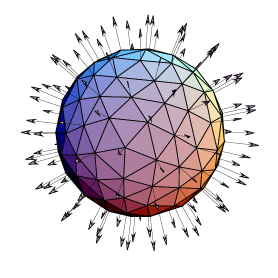
Figure II.1. Hedgehog configuration. Arrows indicate the directions of the isovector field $F(r)$ at different points in coordinate space.

In order to find its generalizations for representations of higher dimension one may compare it to the matrix elements $D_{mn}^{1/2}(\boldsymbol{\alpha})$, and thus obtain the explicit expressions for the Euler angles $\boldsymbol{\alpha}$ in terms of the chiral angle $F(r)$. The result is [49]

$$\alpha^{1} =\varphi-\arctan(\cos\vartheta\,\tan F(r))-\pi/2,$$ (II.II.1.22a)

$$\alpha^{2} =-2\arcsin(\sin\vartheta\,\sin F(r)),$$ (II.II.1.22b)

$$\alpha^{3} =-\varphi-\arctan(\cos\vartheta\,\tan F(r))+\pi/2.$$ (II.II.1.22c)

Here the angles $\varphi,\vartheta$ are the polar angles that define the direction of the unit vector $\bar{}\mathbf{r}$ in spherical coordinates.

Substitution of the expressions (II.II.1.22) into the general expression (II.II.1.4) for the unitary field $\mathbf{U}$ then gives the hedgehog field in a representation with arbitrary $j$. As an example, the hedgehog field in the representation $j=\frac{1}{2}$ has the form [49, 82]

$$\mathbf{U}_{c}^{\frac{1}{2}}=\begin{pmatrix}G&i\sin F\sin\vartheta\mathrm{e}^{-i\varphi}\\ i\sin F\sin\vartheta\mathrm{e}^{i\varphi}&G^{*}\end{pmatrix},$$ (II.II.1.23)

where we have used abbreviation $G=\cos F+i\sin F\cos\vartheta$. For $j=1$ the same substitution yields

$$\mathbf{U}_{c}^{1}=\begin{pmatrix}G^{2}&i\sqrt{2}\sin F\sin\vartheta\mathrm{e}^{-i\varphi}G&-(\sin F\sin\vartheta e^{-i\varphi})^{2}\\ i\sqrt{2}\sin F\sin\vartheta\mathrm{e}^{i\varphi}G&1-2\sin^{2}F\sin^{2}\vartheta&i\sqrt{2}\sin F\sin\vartheta\mathrm{e}^{-i\varphi}G^{*}\\ -(\sin F\sin\vartheta e^{i\varphi})^{2}&i\sqrt{2}\sin F\sin\vartheta\mathrm{e}^{i\varphi}G^{*}&G^{*2}\end{pmatrix}.$$ (II.II.1.24)

The Lagrangian density (II.II.1.17) reduces to the following simple form, when the hedgehog ansatz (II.II.1.22) is employed:

$${\mathscr{L}}=-\frac{4}{3}j(j+1)(2j+1)\bigg{(}\frac{f_{\pi}^{2}}{4}\Bigl{(}F^{\prime 2}+\frac{2}{r^{2}}\sin^{2}\mskip-3.0muF\Bigr{)}\\ +\frac{1}{4e^{2}}\frac{\sin^{2}\mskip-3.0muF}{r^{2}}\Bigl{(}2F^{\prime 2}+\frac{\sin^{2}\mskip-3.0muF}{r^{2}}\Bigr{)}\bigg{)}.$$ (II.II.1.25)

For $j=\frac{1}{2}$ this reduces to the result of Ref. [8]. The corresponding mass density is obtained by reverting the sign of $\mathscr{L}$, as the hedgehog ansatz is a static solution.

The requirement that the soliton mass be stationary yields the following equation for the chiral angle $F(r)$ [8]:

$$f_{\pi}^{2}\Bigl{(}F^{\prime\prime}+\frac{2}{r}F^{\prime}-\frac{\sin 2F}{r^{2}}\Bigr{)}-\frac{1}{e^{2}}\Bigl{(}\frac{1}{r^{4}}\sin^{2}\mskip-3.0muF\,\sin 2F\\ -\frac{1}{r^{2}}(F^{\prime 2}\sin 2F+2F^{\prime\prime}\sin^{2}\mskip-3.0muF)\Bigr{)}=0.$$ (II.II.1.26)

It is independent of the dimension of the representation. Note that the differential equation is nonsingular only if $F(0)=n\pi,\quad n\in\mathds{Z}$.

For the hedgehog form the baryon density reduces to the expression

$$\mathscr{B}^{0}=-\frac{1}{3N\pi^{2}}j(j+1)(2j+1)\frac{\sin^{2}F}{r^{2}}F^{\prime}.$$ (II.II.1.27)

The corresponding baryon number is

$${B}=\int\mathrm{d}^{3}r\mathscr{B}^{0}=\frac{2}{3N\pi}j(j+1)(2j+1)\bigl{(}F(0)-\frac{1}{2}\sin 2F(0)\bigr{)}.$$ (II.II.1.28)

Combining the requirement that $F(0)$ to be an integer multiple of $\pi$ with the requirement that the lowest nonvanishing baryon number to be $1$ gives the general expression for the normalization factor $N$ as

$$N=\frac{2}{3}j(j+1)(2j+1).$$ (II.II.1.29)

The equation of motion for chiral angle in the form (II.II.1.26) depends on parameter $f_{\pi}$ and $e$ values. It is convenient to introduce a dimensionless variable $\tilde{r}=ef_{\pi}r$ in which (II.II.1.26) takes the form

$$F^{\prime\prime}(\tilde{r})\Bigl{(}1+\frac{2\sin^{2}\mskip-3.0muF(\tilde{r})}{\tilde{r}^{2}}\Bigr{)}+F^{\prime 2}(\tilde{r})\frac{\sin 2F(\tilde{r})}{\tilde{r}^{2}}+\frac{2}{\tilde{r}}F^{\prime}(\tilde{r})\\ -\frac{\sin 2F(\tilde{r})}{\tilde{r}^{2}}-\frac{\sin 2F(\tilde{r})\sin^{2}\mskip-3.0muF(\tilde{r})}{\tilde{r}^{4}}=0.$$ (II.II.1.30)

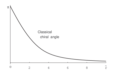
Figure II.2. Classical chiral angle solution, as taken from Ref. [8] ($e=5.45$, $F_{\pi}=129$ MeV, $\tilde{r}=eF_{\pi}r$).

Numerical investigation [6] of (II.II.1.30) leads to classical chiral angle solution $F(\tilde{r})$ shown in Fig. II.2, when boundary conditions $F(0)=\pi,\quad F(\infty)=0$ ensuring baryon number $1$ are imposed.

II.1.5. Higher order terms

There exists an infinite class of alternate stabilizing terms for the Lagrangian density (II.II.1.6), combinations of which can be used in place of Skyrme’s quartic stabilizing term or be added to it [20]. An alternate term of quartic order (which for $j=1/2$ yields the same result as the Skyrme term) is [27]

$${\mathscr{L}}^{\prime}_{4}=\frac{1}{16e^{\prime 2}}\Bigl{(}\operatorname{Tr}\{\mathbf{R}_{\mu}\mathbf{R}_{\nu}\}\operatorname{Tr}\{\mathbf{R}^{\mu}\mathbf{R}^{\nu}\}-(\operatorname{Tr}\{\mathbf{R}_{\mu}\mathbf{R}^{\mu}\})^{2}\Bigr{)}.$$ (II.II.1.31)

When this term is expressed in terms of the Euler angles (II.II.1.3), the resulting Lagrangian density has the form (II.II.1.17), with the exception that the stabilizing term that is proportional to $e^{-2}$ has an additional factor $\frac{2}{3}j(j+1)(2j+1)$ [49]. Hence invariance of the physical predictions requires that the parameter $1/e^{\prime 2}$ of the stabilizing term (II.II.1.31) be taken to be proportional to $\bigl{(}j(j+1)(2j+1)\bigr{)}^{-2}$, and the parameter $f_{\pi}$ of the quadratic term to be proportional to $\bigl{(}j(j+1)(2j+1)\bigr{)}^{-1}$, when a representation of dimension $2j+1$ is employed. Thus, $\mathscr{L}_{4}^{\prime}$ has different representation dependence from a similar term in (II.II.1.6).

Consider then the sixth order stabilizing term [19, 20]

$${\mathscr{L}}_{6}=e_{6}\operatorname{Tr}\{[\mathbf{R}_{\mu},\mathbf{R}^{\nu}][\mathbf{R}_{\nu},\mathbf{R}^{\lambda}][\mathbf{R}_{\lambda},\mathbf{R}_{\mu}]\}.$$ (II.II.1.32)

In terms of the Euler angles $\boldsymbol{\alpha}$ this Lagrangian density takes the form [49]

$${\mathscr{L}}_{6}=-e_{6}{\frac{j(j+1)(2j+1)}{6}}\epsilon_{i_{1}i_{2}i_{5}}\,\epsilon_{i_{3}i_{4}i_{6}}\,\sin^{2}\mskip-3.0mu\alpha^{2}\\ \times\partial_{\mu}\alpha^{i_{1}}\,\partial^{\nu}\mskip-3.0mu\alpha^{i_{2}}\,\partial_{\nu}\alpha^{i_{3}}\partial^{\lambda}\alpha^{i_{4}}\,\partial_{\lambda}\mskip-3.0mu\alpha^{i_{5}}\,\partial^{\mu}\mskip-3.0mu\alpha^{i_{6}}.$$ (II.II.1.33)

This result reveals that the dependence on the dimension of the representation of this term is contained in the same overall factor $j(j+1)(2j+1)$ as in the Skyrme model Lagrangian (II.II.1.17). Hence addition of the term ${\mathscr{L}}_{6}$ maintains the simple overall dimension dependent factor of the original Skyrme model.

As in the case of the quartic term one can construct an alternative sixth order term, which is equivalent to (II.II.1.32) in the case of the fundamental representation, but which differs in its dependence on $j$

$${\mathscr{L}}^{\prime}_{6}=e^{\prime}_{6}\,\epsilon^{\mu\nu_{1}\nu_{2}\nu_{3}}\,\epsilon_{\mu\eta_{1}\eta_{2}\eta_{3}}\,\operatorname{Tr}\{\mathbf{R}_{\nu_{1}}\mathbf{R}_{\nu_{2}}\mathbf{R}_{\nu_{3}}\mathbf{R}^{\eta_{1}}\mathbf{R}^{\eta_{2}}\mathbf{R}^{\eta_{3}}\}.$$ (II.II.1.34)

In terms of the Euler angles $\boldsymbol{\alpha}$ this term also reduces to the expression (II.II.1.33), with the exception of an additional factor $j(j+1)(2j+1)e^{\prime}_{6}/e_{6}$. Its dependence on $j$ is thus different from (II.II.1.32), although by adjusting the values of the parameters $e_{6}$ and $e^{\prime}_{6}$ differently in each representation equivalent dynamical predictions in the classical model can be maintained. Obviously we cannot express (II.II.1.31) and (II.II.1.34) as inner product of group generators, whereas for (II.II.1.33) this should be possible.

II.2. The Lagrangian symmetries

We start from construction of chirally invariant terms of the lowest order, which satisfy additional physical requirements. Maximal symmetry requirement together with $B=1$ condition directly lead to Skyrme hedgehog solution in fundamental representation. This solution then is generalised to any SU(2) representation.

II.2.1. Chiral symmetry breaking

It is commonly accepted that chiral symmetry is the symmetry of QCD (theory of strong interactions) in the zero quark mass limit. There is only one second order chirally invariant term

$$\mathscr{L}_{(2)}\sim\int\operatorname{Tr}\{\mathbf{R}_{\mu}\mathbf{R}^{\mu}\}\mathrm{d}^{3}\mskip-3.0mu\mathbf{x},$$ (II.II.2.1)

whereas there are three linearly independent invariants of the order four [50]

$$\mathscr{L}_{(4)}\sim a\operatorname{Tr}\{\mathbf{R}_{\mu}\mathbf{R}^{\mu}\,\mathbf{R}_{\nu}\mathbf{R}^{\nu}\}+b\operatorname{Tr}\{\mathbf{R}_{\mu}\mathbf{R}_{\nu}\mathbf{R}^{\mu}\mathbf{R}^{\nu}\}+c\operatorname{Tr}\{\partial_{\mu}\mathbf{R}_{\nu}\partial^{\mu}\mathbf{R}^{\nu}\},$$ (II.II.2.2)

$a,b,c$ being some constants. All three of them are Lorenz invariants so there are no reasons to prefer any one of them. But if we want to ensure positive energy density and (as a consequence) to avoid pathology in system dynamics we should take care that time components of "right" currents entered the Lagrangian only in quadratic form. The requirement is satisfied by the only combination of the order four

$$\mathscr{L}_{(4)}=\operatorname{Tr}\{\mathbf{R}_{\mu}\mathbf{R}^{\mu}\,\mathbf{R}_{\nu}\mathbf{R}^{\nu}\}-\operatorname{Tr}\{\mathbf{R}_{\mu}\mathbf{R}_{\nu}\mathbf{R}^{\mu}\mathbf{R}^{\nu}\}=-\frac{1}{2}\operatorname{Tr}\{\bigl{[}\mathbf{R}_{\mu},\mathbf{R}_{\nu}\bigr{]}\bigl{[}\mathbf{R}^{\mu},\mathbf{R}^{\nu}\bigr{]}\},$$ (II.II.2.3)

which is exactly the term suggested by T.H.R. Skyrme. The Lagrangian (II.II.1.6) is invariant under global (point independent) chiral group $SU(2)_{L_{eft}}\otimes SU(2)_{R_{ight}}$ of transformations of unitary field $\mathbf{U}$

$$\mathbf{U}^{\prime}(\mathbf{x})=\mathbf{V}\mathbf{U}(\mathbf{x})\mathbf{W}^{-1};\qquad\mathbf{V}\in SU(2)_{L};\quad\mathbf{W}\in SU(2)_{R}.$$ (II.II.2.4)

The group $SU(2)_{L}\otimes SU(2)_{R}$, however, is not a symmetry group of classical vacuum state (the highest symmetry field from $Q_{0}$ sector which takes on the constant value $\mathbf{1}$)

$$\mathbf{U}(\infty,t)=\mathbf{U}_{vac}(\mathbf{x},t)\equiv\mathbf{1},\quad\text{unless}\quad\mathbf{V}=\mathbf{W}.$$ (II.II.2.5)

As a consequence, maximal global invariant subgroup of configuration space of the model is

$$\operatorname{diag}\bigl{(}SU(2)_{L}\otimes SU(2)_{R}\bigr{)}\approx SU(2)_{I_{sotopic}},$$ (II.II.2.6)

where the standard notation $\operatorname{diag}(G_{1}\otimes G_{2})$ denotes the subgroup of $G_{1}\otimes G_{2}$ with parameters of $G_{1}$ and $G_{2}$ being identified.

II.2.2. Hedgehog ansatz as a lowest energy solution

In the baryon number zero sector the field which takes on the constant value $\mathbf{1}$ is the field of the highest symmetry. It is fully Poincaré invariant and provides a classical description of the vacuum state.

We expect that the ground state for $B=1$ would be described by a configuration $\mathbf{U}$ with the maximal possible symmetry. When the winding number $B$ is not zero, the field $\mathbf{U}$ cannot possess translational invariance. A translational invariant field is a constant and corresponds to $B=0$. When $B\neq 0$, $\mathbf{U}$ cannot be rotationally invariant either. This is because a spherically symmetric unitary field $\mathbf{U}$ depends only on the radial distance $r$

$$\mathbf{U}^{\dagger}\partial_{i}\mathbf{U}=\bar{}\mathbf{x}_{i}\mathbf{U}^{\dagger}\frac{\partial\mathbf{U}}{\partial r},$$ (II.II.2.7)

where $\bar{}\mathbf{x}$ is a unit vector in Cartesian coordinate system. Then

$$\mathscr{B}(\mathbf{U})\sim\epsilon_{ijk}\operatorname{Tr}\{\bigl{(}\mathbf{U}^{\dagger}\partial_{i}\mathbf{U}\bigr{)}\bigl{(}\mathbf{U}^{\dagger}\partial_{j}\mathbf{U}\bigr{)}\bigl{(}\mathbf{U}^{\dagger}\partial_{k}\mathbf{U}\bigr{)}\}=0.$$ (II.II.2.8)

To obtain one with $B\neq 0$ let us blend isotopic rotations $SU(2)_{I}$ with space rotations $\mathrm{SO(3)}$ to form a group $\operatorname{diag}\bigl{(}SU(2)_{I}\otimes\mathrm{SO(3)}\bigr{)}$. The unitary field $\mathbf{U}$ transforms under $\operatorname{diag}\bigl{(}SU(2)_{I}\otimes\mathrm{SO(3)}\bigr{)}$ as follows [86]:

$$\mathbf{U}_{g}(\mathbf{x})=T(g)\mathbf{U}(g^{-1}\mathbf{x})=\mathbf{U}(\mathbf{x});\quad g\in\operatorname{diag}\bigl{(}SU(2)_{I}\otimes\mathrm{SO(3)}\bigr{)}.$$ (II.II.2.9)

Substituting expressions for the explicit rotation generators in the fundamental representation of $SU(2)_{I}$ yields differential equation

$$-i\bigl{(}\mathbf{x}\times\mathbf{\nabla}\bigr{)}_{i}\mathbf{U}(\mathbf{x})+\bigl{[}\frac{\boldsymbol{\tau}_{i}}{2},\mathbf{U}(\mathbf{x})\bigr{]}=0.$$ (II.II.2.10)

The solution of (II.II.2.10) is

$$\mathbf{U}(\mathbf{x})=\mathbf{U}_{c}(\mathbf{x})\equiv\cos F(r)\cdot\mathbf{1}+i\boldsymbol{\tau}\cdot\mathbf{x}\sin F(r).$$ (II.II.2.11)

Pictorially it is illustrated in Fig. II.1, where arrow length $|\sin F(r)|$ (for function $F(r)$ itself see Fig. II.2) goes to zero as $r\rightarrow\infty$ and $r\rightarrow 0$. The solution of (II.II.2.10) is exactly the Skyrme’s hedgehog ansatz (II.II.1.21). Generalization to the arbitrary representation is straightforward. Instead of (II.II.2.10) we have

$$i\bigl{(}\mathbf{x}\times\mathbf{\nabla}\bigr{)}_{i}\mathbf{U}(\mathbf{x})+\sqrt{2}\bigl{[}J_{i},\mathbf{U}(\mathbf{x})\bigr{]}=0,$$ (II.II.2.12)

where circular components (II.II.1.8) are used both for the vector and isovector. The solution of (II.II.2.12) is a generalized hedgehog ansatz

$$\mathbf{U}_{c}(\mathbf{x})=\exp\bigl{(}-i\sqrt{2}\,J_{a}\bar{x}^{a}\,F(r)\bigr{)}.$$ (II.II.2.13)

Sometimes the hedgehog ansatz (II.II.2.11), (II.II.2.13) is referred to as "spherically symmetric" solutions. These solutions are "spherically symmetric" only in the sense that a coordinate rotation is equivalent to an isospin rotation of the constant matrix $\mathbf{A}$

$$\mathbf{U}_{c}(\mathbf{x})=\mathbf{A}\exp\bigl{(}-i\sqrt{2}\,J_{a}\bar{x}^{a}\,F(r)\bigr{)}\mathbf{A^{\dagger}},\quad\mathbf{A}\in SU(2).$$ (II.II.2.14)

To summarize, the highest symmetry solution for $B\neq 0$ sector leads to certain mixing of indices associated with internal and geometric invariance (which are — a priori — completely unrelated). Similar examples are given by the monopole and instanton configurations which occur in SU(2) gauge theories.

"One may wonder whether such a blend of internal and geometric symmetries may exist at a more fundamental level as a general feature of field theory and not simply in specific field configurations of particular models. This feature would be very attractive for the construction of a unified theory of all fundamental interactions including gravity. That this is not possible is expressed by the so called no-go theorems, in particular the theorem of Coleman and Mandula, which essentially says the following: the most general invariance group of a relativistic quantum field theory is a direct product of the Poincaré group and an internal symmetry group, i.e. there is no mixture of these symmetry transformations.

However, these no-go theorems do not claim that such a mixture cannot exist if the set of all symmetry transformations represents a more general algebraic structure than a Lie group. Indeed, a famous result known as the theorem of Haag, Lopuszànski and Sohnius [87] states that the most general super Lie group of local field theory is the N-extended super Poincaré group in which there is a non-trivial mixing of geometric transformations and internal SU(N) transformations. As a matter of fact, this result can also be viewed as a good argument in favour of the existence of supersymmetry as an invariance of nature since it states that supersymmetry is the natural (only possible) symmetry if one allows for super Lie groups as symmetry structures" [88].

The existence of nontrivial mixing for certain configurations in the Skyrme model as well as in supersymmetric models may serve as a strong argument for further investigations of the model which is much more simple to deal with than those of supersymmetric theories.

II.2.3. Higher sectors solutions

It is proved [50] (see, however, [89]) that "spherically symmetric" hedgehog ansatz leads to the absolute energy minimum only when $B=1$. For $B=2$ value of baryon number it is hoped [50] that axial symmetric states

$$F=F(r,\vartheta);\quad\Theta=\Theta(r,\vartheta);\quad\Phi=m\varphi;\qquad m\in\mathds{N},$$ (II.II.2.15)

realise energy minimum configurations. The statement was verified numerically [90, 91]. The value is $E_{B=2}/E_{B=1}=1.92$ for the ratio of energies for axial symmetric solution of sector $B=2$ and spherically symmetric hedgehog ansatz with $B=1$. Energy/baryon densities for $B=2$ configuration possess a toroidal symmetry (see Fig. C.1 in Appendix C). Stable ansatz for $\mathbf{U}$ minimizing energy and with baryon numbers $B\geq 2$ have been numerically found by various groups [17, 23, 92]. Energy densities for these static configurations have been plotted and a remarkable fact has been discovered that they are invariant under discrete subgroups ${\goth G}_{R}$ of the spatial rotation group SO(3). Some of them are shown [23] in Appendix C. The group ${\goth G}_{R}$ is the symmetry group of energy density. It is not necessarily the invariance group of the static $\mathbf{U}$ field. Published work [92] does not report on the symmetry group of the latter.

Configurations with $B>1$ are important in nuclear physics [17] since proton and nuclei could be related to quantized states of these soliton-like fields. Several recent studies support this point of view [16] and suggest that the structures of heavier nuclei could resemble those of fullerene molecules, at least at the classical level.

II.2.4. Reducible representations

Generalization of the model to arbitrary reducible representation is a bit straightforward. One needs only to sum over all irreducible representations involving explicit dependence on representation. Thus, substitution for (II.II.1.4) is

$$\mathbf{U}(\mathbf{r},t)=\sum_{k}\oplus\mathbf{D}^{j_{k}}\left(\boldsymbol{\alpha}(\mathbf{r},t)\right).$$ (II.II.2.16)

The general scalar product (II.II.1.9) then modifies to

$$\operatorname{Tr}\langle j{\cdot}|J_{a}J_{b}|j{\cdot}\rangle=(-1)^{a}\frac{1}{6}\sum_{k}j_{k}(j_{k}+1)(2j_{k}+1)\delta_{a,-b},$$ (II.II.2.17)

and the normalization factor (II.II.1.29) takes a form

$$N=\frac{2}{3}\sum_{k}j_{k}(j_{k}+1)(2j_{k}+1).$$ (II.II.2.18)

Other formulas do not involve changes.

Chapter III Quantum Skyrme model

This chapter contains main results. After brief remarks on quantization problems in curved space we skip to collective coordinate approach and consider the Skyrme Lagrangian quantum mechanically ab initio. Assuming noncommutativity of dynamical variables we calculate expressions of Noether currents, magnetic momenta, axial coupling constant, etc. and numerically evaluate physical quantities using the classical chiral angle solution in various SU(2) representations. These numerical results then are used as starting input for self-consistent quantum chiral angle determination procedure. Numerical results of quantum chiral angle calculations are presented in Appendices A and B.

III.1. Quantization in curved space

The purpose of the section is to remind readers the Dirac method of constrained quantization as well as problems of traditional quantization in curved space. The justification of the actual quantization method is considered without going into details in the last subsection. The section, thus, provides the context for quantization procedure followed further but contains no new material.

III.1.1. General remarks

Questions may be raised concerning the justification for quantizing the Skyrme Lagrangian at all, since it is not a fundamental field theory, but rather a classical model that results from taking the limit of such a theory, including only some degrees of freedom of the original theory. Nevertheless, there is a rich experience from the nonrelativistic many-body problems, for example, from nuclear physics [93], suggesting the validity of such an approach for the study of collective properties at low energies.

The second remark concerns general quantization strategy. At the University level the construction of quantum theory passes three steps, namely Lagrangian (classical) $\rightarrow$ Hamiltonian (classical) $\rightarrow$ Hamiltonian (quantum) $\equiv$ Quantum theory. The quantization in collective coordinate approach [48], which we will follow in the work, slightly modifies this sequence. It starts from the quantum Lagrangian from the outset. By quantum Lagrangian we mean that dynamical coordinates $q^{i}$ and its time derivatives (velocities) $\dot{q}^{i}$ do not commute. The explicit commutation relations at the moment are unknown. These relations are extracted from the standard commutation relations $[q^{i},p^{j}]$ after we pass to quantum Hamiltonian (and define canonical momenta $p^{j}$). It can be shown that this modified formalism [94, 95, 96] leads to consistent quantum description, which we will follow in subsequent sections.

The results of modified and usual quantization sequences generally will differ. Noncommuting quantum variables will generate additional terms while passing from quantum Lagrangian to quantum Hamiltonian. These terms are lost when we impose canonical commutation relations after Hamiltonian is obtained. The problem is similar to well known operator ordering problem. Further in the work we will refer to "canonical quantization method" when we start from quantum Lagrangian in the very beginning and to "semiclassical quantization method" when canonical commutation relations are imposed after Hamiltonian is calculated. It should be noted, however, that these two choices do not use up all possibilities. In Ref. [31], for example, the following possibilities are discussed:

$$\begin{array}[]{ccccc}L_{\text{Skyrme}}(\mathbf{\Phi},\dot{\mathbf{\Phi}})&\Longrightarrow&L_{\text{hedg.}}(F,\dot{F},\mathbf{A},\dot{}\mathbf{A})&\Longrightarrow&L_{\text{coll.}}(\mathbf{q},\dot{}\mathbf{q})\\ \Downarrow\text{case I}&&\Downarrow\text{case II}&&\Downarrow\text{case III}\\ \hat{H}_{\text{Skyrme}}(\mathbf{\Phi},\mathbf{\pi})&\Longrightarrow&\hat{H}_{\text{hedg.}}(F,\mathbf{\Pi}_{F},\mathbf{A},\mathbf{\Pi}_{A})&\Longrightarrow&\hat{H}_{\text{coll.}}(\mathbf{q},\dot{}\mathbf{p})\\ \end{array}.$$ (III.III.1.1)

In case I, the Hamiltonian gets by quantizing directly the Lagrangian in the Skyrme model from the beginning. After this quantization one can introduce the hedgehog ansatz and the collective coordinates. As another method (case II) we can do the quantization of the classical Lagrangian, which is obtained by introducing the hedgehog ansatz and after this we introduce the collective coordinates. Case III starts by getting the classical Lagrangian with the collective coordinates, using the hedgehog ansatz and getting the quantum Hamiltonian. The case II is free of the ordering problem among the operators. However, in both cases I and III, there are the ordering problems among the operators, and then quantum Hamiltonian cannot been determined uniquely. In summary, the problem is in which steps we do the quantization. Following [48] we utilize the following detailed quantization sequence:

1. Introduce quantum collective coordinates $\mathbf{A\bigl{(}\mathbf{q}(t)\bigr{)}}$ (III.III.2.1). They are quantum in the sense that time differentiation of $\mathbf{A}$ requires the Weyl ordering (see Sec. III.1.4).

2. Make the Lagrangian quantum. Quantum dynamical variables are $\mathbf{q}(t)$.

3. Following the method described in [48, 94, 95, 96, 97, 98, 99] pass to quantum Hamiltonian.

4. Introduce the hedgehog ansatz, and solve integro-differential equation for quantum chiral angle.

Another important point is symmetry properties of classical Lagrangian and quantum Hamiltonian derived from it. There exist quantization methods (for example, general covariant Hamiltonian method [42]) preserving original classical Lagrangian symmetries. The symmetric (Weyl) ordering of operators $\mathbf{q}$ and $\mathbf{p}$ (used in the work), however, cannot avoid a risk that the quantum Hamiltonian has chiral symmetry breaking term [31]. The feature thus can be used to provide (or explain) the origin of finite pion mass.

The subsections below are intended to shed a bit light on the justification of the quantization method we will follow.

III.1.2. Towards quantum theory

There where attempts [100] to quantize classical equations of motion in the form

$$m\frac{\mathrm{d}^{2}x^{i}}{\mathrm{d}t^{2}}=f^{i},$$ (III.III.1.2)

without resort to a Lagrangian (or Hamiltonian). The idea is to start with classical equations (III.III.1.2) and give commutation relations for the operators $X^{i}$ and $\dot{X}^{j}$

$$\bigl{[}X^{i},X^{j}\bigr{]} =0$$ (III.III.1.3a)

$$\bigl{[}X^{i},\dot{X}^{j}\bigr{]} =i\hbar\delta^{i,j}.$$ (III.III.1.3b)

The result was that the existence of Lagrangian for (III.III.1.2) essentially comes from (III.III.1.3a). Thus Feynman’s hope to quantize without a Lagrangian (or Hamiltonian) was doomed when he set the very reasonable condition that coordinates commute [101]. Let us briefly review traditional quantization methods following Ref. [102].

III.1.3. Traditional quantization methods

We will mention four of them here in the order of historical evolution.
Heisenberg quantization is based on the following postulates (for the first postulate see below):

1. Introduce matrices $\mathbf{Q}=\{Q_{mn}\}$ and $\mathbf{P}=\{P_{mn}\}$, here $m,n\in\{1,2,3,\ldots\}$, that satisfy $[\mathbf{Q},\mathbf{P}]_{mn}\equiv{\displaystyle\sum_{p}}(Q_{mp}P_{pn}-P_{mp}Q_{pn})=i\hbar\delta_{m,n}$.

2. Build a Hamiltonian matrix $\mathbf{H}=\{H_{mn}\}$ as a function (e.g., polynomial) of the matrices, $H_{mn}=H(\mathbf{P},\mathbf{Q})_{mn}$, that is the same function as the classical Hamiltonian $H(p,q)$. (In so doing there may be operator ordering ambiguities which this prescription cannot resolve; choose an ordering that leads to a Hermitian operator.)

3. Introduce the equation of motion $i\hbar{\dot{X}}_{mn}=[\mathbf{X},\mathbf{H}]_{mn}$ for the elements of a general matrix $\mathbf{X}=\{X_{mn}\}$.

Along with these postulates comes the implicit task of solving the above equations of motion subject to suitable operator-valued boundary conditions. After the principal paper on quantization [103], it subsequently became clear to W. Heisenberg that it is necessary to make this promotion from $c$-number to $q$-number variables only in Cartesian coordinates. Thus here is implicitly another postulate [104]:

1. Express the classical kinematical variables $p$ and $q$ in Cartesian coordinates prior to promoting them to matrices $\{P_{mn}\}$ and $\{Q_{mn}\}$, respectively.

Schrödinger quantization assumes the following postulates [105]:

1. Express the classical kinematical variables $p$ and $q$ in Cartesian coordinates.

2. Promote the classical momentum $p$ to the differential operator $-i\hbar(\partial/\partial q)$ and the classical coordinate $q$ to the multiplication operator $\hat{q}$, a choice that evidently satisfies the commutation relation $[\hat{q},-i\hbar(\partial/\partial q)]=i\hbar$.

3. Define the Hamiltonian operator $\hat{H}$ as the classical Hamiltonian with the momentum variable $p$ replaced by the operator $-i\hbar(\partial/\partial q)$ and the coordinate variable $q$ replaced by the operator $\hat{q}$. (In so doing there may be operator ordering ambiguities which this prescription cannot resolve; choose an ordering that leads to a Hermitian operator.)

4. For $\psi(q)$ a complex, square integrable function of $q$, introduce the dynamical equation $i\hbar{\dot{\psi}}=\hat{H}\psi$.

Implicit with these postulates is the instruction to solve the Schrödinger equation for a dense set of initial conditions and a large class of Hamiltonian operators. It is interesting to note that E. Schrödinger himself soon became aware of the fact that his procedure generally works only in Cartesian coordinates.
Dirac quantization recipe deals with constrained dynamical systems. Constrains appear in the Hamilton formulation of all gauge theories we know of. Dirac-Bergmann constraint theory puts all these constraints into first or second classes. All second class constraints $S_{a}$ can be eliminated from the theory, whereas Dirac prescription for the implementation of first class constraints $F_{a}$ in quantum theory is that they be imposed as conditions on the physically allowed states $|{\cdot}\rangle$:

$$\hat{F}_{a}|{\cdot}\rangle=0.$$ (III.III.1.4)

Here $\hat{F}_{a}$ is the quantum operator corresponding to the classical function $F_{a}$.
Feynman quantization focuses on the solution to the Schrödinger equation and postulates that the propagator, an integral kernel that maps the wave function (generally in the Schrödinger representation) at one time to the wave function at a later time, may be given by means of a path integral expression [106]. On the surface, it would seem that the (phase space) path integral, using only concepts from classical mechanics, could get around the need for Cartesian coordinates. That is not the case [107]. As postulates for a path integral quantization scheme we have:

1. Express the classical kinematical variables $p$ and $q$ in Cartesian coordinates.

2. Given that $|q,t\rangle$, where $Q(t)|q,t\rangle=q|q,t\rangle$, denote sharp position eigenstates, write the transition matrix element in the form of a path integral as

   $$\langle q^{\prime\prime},T|q^{\prime},0\rangle=\mathscr{M}\int\exp\Bigl{(}(i/\hbar)\int\bigl{(}p{\dot{q}}-\hat{H}(p,q)\bigr{)}\,\mathrm{d}t\Bigr{)}\,\mathscr{D}p\,\mathscr{D}q.$$ (III.III.1.5)

3. Recognize that the formal path integral (III.III.1.5) is effectively undefined and replace it by a regularized form of path integral, namely,

   $$\langle q^{\prime\prime},T|q^{\prime},0\rangle=\lim_{N\rightarrow\infty}M_{N}\int\exp\Bigl{(}\frac{i}{\hbar}{\displaystyle\sum_{l=0}^{N}}\bigl{(}p_{l+\scriptscriptstyle 1/2}(q_{l+1}-q_{l})\\ -\frac{\epsilon}{2}\hat{H}(p_{l+\scriptscriptstyle 1/2},q_{l+1}+q_{l})\bigr{)}\Bigr{)}\,\Pi_{l=0}^{N}\mathrm{d}p_{l+\scriptscriptstyle 1/2}\,\Pi_{l=1}^{N}\mathrm{d}q_{l},$$ (III.III.1.6)

   where $q_{N+1}=q^{\prime\prime}$, $q_{0}=q^{\prime}$, $M_{N}=(2\pi\hbar)^{-(N+1)}$, $p_{l+\scriptscriptstyle 1/2}=(p_{l}+p_{l+1})/2$, and $\epsilon=T/(N+1)$.

Implicit in the latter expression is a Weyl ordering choice to resolve any operator ordering ambiguities. Observe that the naive lattice formulation of the classical action leads to correct quantum mechanical results, generally speaking, only in Cartesian coordinates. Although the formal phase space path integral (III.III.1.5) appears superficially to be covariant under canonical coordinate transformations, it would be incorrect to conclude that was the case inasmuch as it would imply that the spectrum of diverse physical systems would be identical. In contrast, the naive lattice prescription applies only to Cartesian coordinates, the same family of coordinates singled out in the first postulate of each of the previous quantization schemes.

It is essential that traditional quantization methods start from global Cartesian coordinate system and Hamiltonian function. But if we want Lorenz covariant theory, then it is not a good idea to start formulation from the Hamiltonian as there are no easy ways to ensure Lorenz covariance. The easiest way to get Lorenz covariant theory is to start formulation from Lorenz invariant Lagrangian. This way leads us directly both to Hamilton formulation and operator ordering problems.

III.1.4. Weyl ordering

A path integral formalism sometimes is referred to as a quantum method resolving the operator ordering problem [110]. This is because the Weyl ordered expressions are used in the regularized form (III.III.1.6) of a path integral in order to resolve the ambiguities.

Let us illustrate the problem for an unconstrained system. Namely, let us recall the well known harmonic oscillator example. The problem is that two identical classical Hamiltonians

$$H_{1} \sim x^{2}+p^{2}; \qquad H_{2} \sim(x-ip)(x+ip),$$ (III.III.1.9a)

lead to different energies in quantum theory

$$E_{1} \sim\hbar\omega(n+\frac{1}{2});\qquad\text{and} \qquad E_{2} \sim\hbar\omega n,$$ (III.III.1.9b)

respectively, when the same commutation relations $[\hat{p},\hat{q}]$ is imposed. The reason is that the two quantum Hamiltonians (III.III.1.9a) differ exactly by the commutator $[\hat{p},\hat{q}]$, what is indicated by additional $\frac{1}{2}\hbar\omega$ term in the system energy. The Weyl ordered Hamiltonian $H_{1}$ results to the true energy $\hbar\omega(n+\frac{1}{2})$. How can Weyl ordering can be applied in the general case?

Because of nonvanishing commutator $[\dot{q},q]\neq 0$ we need to state more explicitly what we understand under the symbol $\partial_{t}G(q)$. The most natural seems to be the definition

$$\bigl{(}\partial_{t}G(q)\bigr{)}_{W_{\text{eyl ordering}}}=\frac{1}{2}\Bigl{\{}\dot{q},\,\frac{\mathrm{d}G(q)}{\mathrm{d}q}\Bigr{\}},$$ (III.III.1.10)

which is a consequence of application of the Newton-Leibnitz rule to Taylor series expansion of arbitrary function $G(q)$,

$$G(q)=G(q_{0})+G^{\prime}(q)\Bigl{|}_{q=q_{0}}\,q+\frac{1}{2}G^{\prime\prime}(q)\Bigl{|}_{q=q_{0}}\,q^{2}+\dotsb.$$ (III.III.1.11)

Indeed,

$$(\partial_{t}q^{2})_{W}=\partial_{t}(q\,q)=\dot{q}q+q\dot{q}=\frac{1}{2}\{\dot{q},\,\frac{\mathrm{d}(q^{2})}{\mathrm{d}q}\},$$ (III.III.1.12a)

$$(\partial_{t}q^{3})_{W}=\partial_{t}(q\,q\,q)=\dot{q}q^{2}+q\dot{q}q+q^{2}\dot{q}=\frac{3}{2}(\dot{q}q^{2}+q^{2}\dot{q})=\frac{1}{2}\{\dot{q},\,\frac{\mathrm{d}(q^{3})}{\mathrm{d}q}\},$$ (III.III.1.12b)

$$(\partial_{t}q^{n})_{W}=\partial_{t}\underbrace{(q\dots q)}_{n}=\underbrace{\dot{q}q+\dotsb+q\dot{q}}_{n}=\frac{1}{2}\Bigl{\{}\dot{q},\,\frac{\mathrm{d}q^{n}}{\mathrm{d}q}\Bigr{\}}.$$ (III.III.1.12c)

Here the notation $(\partial_{t}q^{n})_{W}$ is related to the usual Weyl ordering notation $(a^{n}b)_{W}$ in an obvious way

$$\frac{1}{n}\bigl{(}\partial_{t}q^{n}\bigr{)}_{W}=\bigl{(}q^{n-1}\dot{q}\bigr{)}_{W}\ .$$ (III.III.1.13)

The general Weyl ordered term $(q^{n}\dot{q})_{W_{1}}$ has a form

$$(q^{n}\dot{q})_{W_{1}}=\frac{1}{n+1}\sum_{l=0}^{n}q^{n-l}\dot{q}q^{l}.$$ (III.III.1.14)

It is straightforward to prove [111] that the above form of Weyl ordering is identical to the definition

$$(q^{n}\dot{q})_{W_{2}}=(\frac{1}{2})^{n}\sum_{l=0}^{n}\frac{n!}{l!(n-l)!}q^{n-l}\dot{q}q^{l}.$$ (III.III.1.15)

The Weyl ordering has a number of interesting features [110] and is widely used. Further in the work we will follow definition $(q^{n}\dot{q})_{W_{1}}$, which is identical to (III.III.1.10) form.

III.1.5. Hamilton formulation

Passage from Lagrangian to Hamiltonian sometimes requires additional assumptions. Important class of theories, where standard Hamiltonization fails, is, for example, nonlinear models of elementary particles, including the Skyrme model.

Let us concentrate on Lagrangian theories only, namely on local Lagrangian theories of the form

$$L=\int\mathscr{L}(\phi,\partial_{\mu}\phi)\mathrm{d}^{n}\mathbf{x},$$ (III.III.1.16)

allowing non-ambiguous equations of motion. All Lagrangians can be classified into two large groups, depending the system Hessian

$$M_{ij}=\frac{\partial^{2}\mathscr{L}}{\partial\dot{q}^{i}\partial\dot{q}^{j}},$$ (III.III.1.17)

is singular or not. In the case of nonsingular Hessian the usual method of Hamilton formulation is valid [112].

III.1.6. Singular theories

When $M_{ij}$ is a singular matrix ($\det M_{ij}=0$), then we cannot express all velocities $\dot{}\mathbf{q}$ as functions of momenta $\mathbf{p}$ and coordinates $\mathbf{q}$. To show this we simply rewrite Lagrange second order equations

$$\frac{\delta S}{\delta q^{i}}=\frac{\partial\mathscr{L}}{\partial q^{i}}-\frac{\mathrm{d}}{\mathrm{d}t}\frac{\partial\mathscr{L}}{\partial\dot{q}^{i}}=0;\quad S=\int\mathscr{L}\mathrm{d}t,$$ (III.III.1.18)

into two first order equations

$$M^{v}_{ij}\dot{v}^{j}=K^{v}_{i},\qquad\dot{q}^{i}=v^{i},$$ (III.III.1.19)

where the upper index $v$ means that all $\dot{}\mathbf{q}$ are changed to $\mathbf{v}$. It is easy to see that the passage from Lagrangian to Hamiltonian is just variables exchange $(\mathbf{q},\mathbf{v})\rightarrow(\mathbf{q},\mathbf{p})$. The exchange Jacobian is

$$\frac{D(\mathbf{q},\mathbf{v})}{D(\mathbf{q},\mathbf{p})}=\frac{1}{\det\Bigl{\|}\frac{\partial^{2}\mathscr{L}^{v}}{\partial v^{i}\partial v^{j}}\Bigr{\|}},$$ (III.III.1.20)

and, therefore should differ from zero. It is a simple task to check wheather Skyrme Lagrangian is singular or not. This depends on parametrization. In the Euler-Rodrigues parametrization (II.II.1.1) we can express one differential as a function of others, because of the constraint (II.II.1.2) on the fields. Thus we have singular theory in Euler-Rodrigues parametrization, whereas Hessian is clearly nonsingular in Euler angles parametrization (II.II.1.3).

III.1.7. Dirac-Bergmann theory of constraints

Let ${\goth M}$ be the space of "coordinates" appropriate to a Lagrangian $L$. We denote the points of ${\goth M}$ by $\mathbf{q}=(q_{1},q_{2},\dots)$. Now given any manifold ${\goth M}$, it is possible to associate two spaces $TM$ and $T^{*}M$ to ${\goth M}$. The space $TM$ is called the tangent bundle over ${\goth M}$. The coordinate of a point $(\mathbf{q},\dot{}\mathbf{q})$ of $TM$ can be interpreted as a position and a velocity. The Lagrangian is a function on $TM$. The space $T^{*}M$ is called the cotangent bundle over ${\goth M}$. The coordinate of a point $(\mathbf{q},\mathbf{p})$ of $T^{*}M$ can be interpreted as a coordinate and a momentum. At each point $\mathbf{q}$, momenta $\mathbf{p}$ belongs to the vector space dual to the vector space of velocities. Now given a Lagrangian $L$, there exists a map from $TM$ to $T^{*}M$ defined by

$$(\mathbf{q},\dot{}\mathbf{q})\rightarrow\biggl{(}\mathbf{q},\frac{\partial L(\mathbf{q},\dot{}\mathbf{q})}{\partial\dot{}\mathbf{q}}\biggr{)}.$$ (III.III.1.21)

If this map is globally one to one and onto, the image of $TM$ is $T^{*}M$ and we can express velocity as a function of position and momentum (see also previous section). This is the case in elementary mechanics and leads to the familiar rules for the passage from Lagrangian to Hamiltonian mechanics. It may happen, however, that the image of $TM$ under the map (III.III.1.21) is not all of  $T^{*}M$. Suppose, for instance, that it is a submanifold of $T^{*}M$ defined by the equations

$$P_{a}(\mathbf{q},\mathbf{p})=0;\quad a=1,2,\dots.$$ (III.III.1.22)

Then we are dealing with a theory with constraints. The constraints $P_{a}$ are said to be primary.

The functions $P_{a}$ do not identically vanish on $T^{*}M$: their zeros define a submanifold of $T^{*}M$. A reflection of the fact that $P_{a}$ are not zero functions on $T^{*}M$ is that there exist functions $G$ on $T^{*}M$ such that their Poisson brackets $\{G,P_{a}\}$ do not vanish on the surface $P_{a}=0$. These functions $G$ generate canonical transformations which take a point of the surface $P_{a}=0$ out of this surface. It follows that it is incorrect to take Poisson brackets of arbitrary functions with both sides of the equations $P_{a}=0$ and equate them. This fact is emphasized by rewriting (III.III.1.22), replacing the "strong" equality signs $=$ of these equations by "weak" equality signs $\approx$: $P_{a}\approx 0$. When $P_{a}(\mathbf{q},\mathbf{p})$ are weakly zero, we can in general set $P_{a}(\mathbf{q},\mathbf{p})$ equal to zero only after evaluating all Poisson brackets.

In the presence of constraints, the Hamiltonian can be shown to be [114, 115]

$$H =\dot{q}_{a}\frac{\partial L(\mathbf{q},\dot{}\mathbf{q})}{\partial\dot{q}_{a}}-L(\mathbf{q},\dot{}\mathbf{q})+V_{a}P_{a}(\mathbf{q},\mathbf{p})$$ (III.III.1.23a)

$$=H_{0}+V_{a}P_{a}(\mathbf{q},\mathbf{p}).$$ (III.III.1.23b)

In obtaining $H_{0}$ from the first two terms of the first line, one can freely use the primary constrains. The functions $V_{a}$ are as yet undetermined Lagrange multipliers. Some of them may get determined later in the analysis while the remaining ones will continue to be unknown with even their time dependence arbitrary.

Consistency of dynamic requires that the primary constrains are preserved in time. Thus we require that

$$\bigl{\{}P_{a},H\bigr{\}}\approx 0.$$ (III.III.1.24)

These equations may determine some of the $V_{a}$ or they may hold identically when the constraints $P_{a}\approx 0$ are imposed. Yet another possibility is that they lead to the "secondary constraints" $P^{\prime}_{a}(\mathbf{q},\mathbf{p})\approx 0$. The requirement $\bigl{\{}P^{\prime}_{a},H\bigr{\}}\approx 0$ may determine more of the Lagrange multipliers, lead to tertiary constraints or be identically satisfied when (III.III.1.24) and $P^{\prime}_{a}\approx 0$ are imposed. We proceed in this fashion until no more new constraints are generated.

Let us denote all the constraints one obtains in this way by $C_{b}\approx 0$. Dirac divides these constraints into the first and the second class constraints. First class constraints $F_{a}\approx 0$ are those for which $\bigl{\{}F_{a},C_{b}\bigr{\}}\approx 0,\quad\forall b$. In other words, the Poisson brackets of $F_{a}$ with $C_{b}$ vanish on the surface defined by $C_{b}\approx 0$. The remaining constraints $S_{a}$ are defined to be second class. It can be shown that

$$\bigl{\{}F_{a},F_{b}\bigr{\}}=C^{c}_{ab}F_{c},$$ (III.III.1.25)

where $C^{c}_{ab}=-C^{c}_{ba}$ are functions on $T^{*}M$. The proof can be found in [113, 114].

Let ${\goth C}$ be the submanifold of $T^{*}M$ defined by the constraints:

$${\goth C}=\bigl{\{}(\mathbf{q},\mathbf{p})|C_{b}(\mathbf{q},Bp)=0\bigr{\}}.$$ (III.III.1.26)

Then since the canonical transformations generated by $F_{a}$ preserve the constraints, a point of ${\goth C}$ is mapped onto another point of ${\goth C}$ under the canonical transformations generated by $F_{a}$. Since the canonical transformations generated by $S_{a}$ do not preserve the constraints, such is not the case for $S_{a}$. Second class constraints can be eliminated by introducing the so-called Dirac brackets. They have the basic property that the Dirac bracket of $S_{a}$ with any function on $T^{*}M$ is weakly zero. Let ${\goth F}$ be the set of all functions which have zero Poisson brackets with $S_{a}$. So long as we work with only such functions, we can use the constraints $S_{a}\approx 0$ as strong constraints $S_{a}=0$. Assuming that there are no first class constraints, the number $n$ of functionally independent functions ${\goth F}$ is $\dim(T^{*}M)-s$, $s$ being number of second class constraints. Thus $s$ second class constraints eliminate $s$ variables. Since matrix $(\bigl{\{}S_{a},S_{b}\bigr{\}})$ is nonsingular and antisymmetric, $s$ is even. Since $\dim(T^{*}M)$ is even as well, $n$ is even.

Let us apply this theory to the Skyrme model [43]. In Euler-Rodrigues parametrization (II.II.1.1) we have primary constraint (II.II.1.2)

$$S_{1}=\Phi_{a}\Phi_{a}-1=0;\quad a=1,2,3,4.$$ (III.III.1.27a)

The further requirement that the condition (III.III.1.27a) not vary in time can be satisfied by imposing a secondary constraint

$$S_{2}=\Phi_{a}M_{ab}\dot{\Phi}_{b}-1=0;\quad a,b=1,2,3,4\quad,$$ (III.III.1.27b)

where $M_{ab}$ is inertia density matrix in Euler-Rodrigues parametrization explicit form of which is not important for further consideration (see [43] for details). It can be shown (using the canonical equations of motion) that this secondary constraint is independent of time [43]. These two constrains (III.III.1.27) are of the second class, because Poisson bracket of the fields $S_{1}$ and $S_{2}$ is non-vanishing. This is also consistent with the fact that second class constraints come in pairs.

If one carries out a canonical quantization by the usual commutators, trouble ensues from this noncommutativity $\bigl{[}S_{1},S_{2}\bigr{]}_{\text{PB}}\neq 0$. The quantum expression of the constraints is that every vector in Hilbert space must be annihilated by the constraint operators $\hat{S}_{1}$ and $\hat{S}_{2}$. It follows trivially that every vector must also be annihilated by their commutator and this conclusion is inconsistent since the commutator in question is itself nonvanishing in the canonical quantization. One resolution of this difficulty is to introduce modified classical brackets, the Dirac brackets, which share with the Poisson brackets all its basic algebraic properties, but are designed so that the Dirac bracket of any pair of second class constraints vanishes, in our case, $\bigl{[}S_{1},S_{2}\bigr{]}_{\text{DB}}=0$. The Dirac brackets replace the Poisson brackets for determining the time evolution of relevant quantities. This replacement also eliminates the need to introduce a Lagrange multiplier field.

It can be shown [115] that for second class constraints there exists a canonical transformation leading to complete elimination of dependent dynamical variables. By canonical transformation here we mean non-singular transformation of dynamical variables $\boldsymbol{\eta}\rightarrow\boldsymbol{\eta}^{\prime},\quad\boldsymbol{\eta}\equiv(\mathbf{q},\mathbf{p});\quad\boldsymbol{\eta}^{\prime}\equiv(\mathbf{q}^{\prime},\mathbf{p}^{\prime})$ if for arbitrary functions $G_{1}(\boldsymbol{\eta})$ and $G_{2}(\boldsymbol{\eta})$ Poisson brackets are invariant in the following sense

$$\bigl{\{}G_{1}(\boldsymbol{\eta}),G_{2}(\boldsymbol{\eta})\bigr{\}}=\bigl{\{}G^{\prime}_{1}(\boldsymbol{\eta}^{\prime}),G^{\prime}_{2}(\boldsymbol{\eta}^{\prime})\bigr{\}},\quad G^{\prime}_{i}(\boldsymbol{\eta}^{\prime})=G_{i}(\boldsymbol{\eta}),\quad i=1,2.$$ (III.III.1.28)

Note, however, that finding this eliminating transformation is nontrivial task, general solution of which is unknown [115]. Dirac brackets in these new variables $\boldsymbol{\eta}^{\prime}$ coincide with Poisson brackets. In the SU(2) Skyrme model this elimination fortunately can easy be done by introducing Euler angles parametrization.

In SU(3) Skyrme model the problem cannot be completely solved by appropriate parametrization, because of the first class constraints appearance in the theory. In this case Dirac prescription for dealing with first class constraints should be followed. Quantization of SU(3) Skyrme model is also complicated by Wess-Zumino term, which eliminates an extra discrete symmetry that is not a symmetry of QCD [29, 30, 116]. Wess-Zumino term, however, vanishes in the SU(2) case even in quantum model [49].

To summarize, despite Dirac quantization (with its constraints classification into primary/secondary/tertiary/$\dots$, first/second class) is convenient and traditionally often followed, it is, in fact not mandatory [112], due to existence [115] of canonical transformations (III.III.1.28), which eliminate dependent dynamical variables. If this elimination is technically formidable task, then Dirac procedure provides us with consistent quantization method. Euler angles (II.II.1.3) parametrization automatically eliminates dependent dynamical variables, and thus is consistent with Dirac prescription.

III.2. Quantization of skyrmion in collective coordinate approach

The section deals with quantization of the "zero frequency modes" or "collective coordinates" of the classical skyrmion. We proceed here (as in the classical case) with arbitrary irreducible representation. The case of reducible representation is investigated in the last subsection.

III.2.1. Collective coordinate approach

An approximation of "zero modes" or "collective coordinates", which retains just a few modes out of a possible infinite number of modes, requires justification. It has been the subject of some criticism. We shall, however, proceed with our calculations using this approximation.

Following G.S. Adkins et al. [8] we shall employ collective rotational coordinates to separate the variables which depend on the time and spatial coordinates

$$\mathbf{U}\bigl{(}\mathbf{x},\mathbf{q}(t)\bigr{)}=\mathbf{A}\bigl{(}\mathbf{q}(t)\bigr{)}\mathbf{U}_{c}(\mathbf{x})\mathbf{A}^{\dagger}\bigl{(}\mathbf{q}(t)\bigr{)},\qquad\mathbf{A}\bigl{(}\mathbf{q}(t)\bigr{)}\in SU(2)_{I}.$$ (III.III.2.1)

Three real independent parameters $\mathbf{q}(t)=\bigl{(}q^{1}(t),q^{2}(t),q^{3}(t)\bigr{)}$ are dynamical quantum variables — skyrmion rotation (Euler) angles in the internal (isotopic) space $SU(2)_{I}=\operatorname{diag}\bigl{(}SU(2)_{L}\otimes SU(2)_{R}\bigr{)}$ but not in geometric space $\mathrm{SO(3)}$. The skyrmion remains static in geometric space.

Quantum fluctuations near the classical solution can be put into two different classes. Namely, fluctuation modes which are generated by action or Hamiltonian symmetries and modes orthogonal to the symmetric one. Symmetric fluctuation modes are of primary importance in quantum description because the infinitely small energy perturbation can lead to reasonable deviations from classical solution. As a consequence, collective rotation matrices $\mathbf{A}(t),\mathbf{A^{\dagger}}(t)$ in (III.III.2.1) are not required to be small (i.e. close to the identity matrix).

III.2.2. Commutation relations

We shall consider the Skyrme Lagrangian (II.II.1.6) quantum mechanically ab initio. The generalized coordinates $\mathbf{q}(t)$ and velocities $\dot{}\mathbf{q}(t)$ then satisfy the commutation relations

$$\bigl{[}\dot{q}^{r},\,q^{k}\bigr{]}=-ig^{rk}(\mathbf{q}).$$ (III.III.2.2)

Here the tensor $g^{rk}(\mathbf{q})$ is a function of generalized coordinates $\mathbf{q}$ only, the explicit form of which is determined after the quantization condition has been imposed. The tensor $g^{rk}$ is symmetric with respect to interchange of the indices $r$ and $k$ as a consequence of the commutation relation $[q^{r},\,q^{k}]=0$. Indeed, differentiation of the relation gives $[\dot{q}^{r},\,q^{k}]=[\dot{q}^{k},\,q^{r}]$, from what it follows that $g^{rk}$ is symmetric. The commutation relation between a generalized velocity component $\dot{q}^{k}$ and arbitrary function $G(\mathbf{q})$ is given by

$$\bigl{[}\dot{q}^{k},\,G(\mathbf{q})\bigr{]}=-i\sum_{r}g^{kr}(\mathbf{q})\frac{\partial}{\partial q^{r}}G(\mathbf{q}).$$ (III.III.2.3)

We shall employ the Weyl ordering for the noncommuting operators $$\dot{}\mathbf{q},G(\mathbf{q})$$ throughout

$$\partial_{t}G(\mathbf{q})=\frac{1}{2}\Bigl{\{}\dot{q}^{r},\,\frac{\partial G(\mathbf{q})}{\partial q^{r}}\Bigr{\}},$$ (III.III.2.4)

where symbol $\partial_{t}G(\mathbf{q})$ further in the work is understood as $\bigl{(}\partial_{t}G(\mathbf{q})\bigr{)}_{W}$. The operator ordering is fixed by the form of the classical Lagrangian (II.II.1.6) and no further ambiguity associated with it appears at the level of the Hamiltonian. In order to find the explicit form of $g^{rk}(\mathbf{q})$ one can substitute (III.III.2.1) into (II.II.1.6) and keep only terms quadratic in velocities

$$\hat{L}(\dot{}\mathbf{q},\mathbf{q},F)= \frac{1}{N}\int\ \hat{\mskip-3.0mu\mskip-3.0mu\mskip-3.0mu\mathscr{L}}\bigl{(}\mathbf{x},\dot{}\mathbf{q}(t),\mathbf{q}(t),F(r)\bigr{)}r^{2}\sin\vartheta\mathrm{d}r\mathrm{d}\vartheta\mathrm{d}\varphi$$

$$= \frac{1}{2}\dot{q}^{r}g_{rk}(\mathbf{q})\dot{q}^{k}+\text{$(\dot{}\mathbf{q})^{0}$-order term},$$ (III.III.2.5)

where

$$N= \frac{2}{3}j(j+1)(2j+1),$$ (III.III.2.6)

and we introduce here from the very beginning a normalization factor in the Lagrangian (II.II.1.6) in order to ensure baryon number $1$. The $3\times 3$ metric tensor $g_{rk}(\mathbf{q})$ is defined [49] as the scalar product of a set of functions (II.II.1.14) $C_{r}^{(m)}(\mathbf{q})$ or $C_{r}^{\prime(m)}(\mathbf{q})$

$$g_{rk}(\mathbf{q}) =-\frac{1}{2}a(F)\sum_{m}(-)^{m}C_{r}^{(m)}(\mathbf{q})C_{k}^{(-m)}(\mathbf{q})=-\frac{1}{2}a(F)\sum_{m}(-)^{m}C_{r}^{\prime(m)}(\mathbf{q})C_{k}^{\prime(-m)}(\mathbf{q})$$

$$=a(F)\delta_{r,k}+a(F)(\delta_{r,1}\delta_{k,3}+\delta_{r,3}\delta_{k,1})\cos q^{2},$$ (III.III.2.7)

where $a(F)$ (soliton inertia moment) is the following integral:

$$a(F) =\int\mathrm{d}^{3}\mathbf{x}\mathscr{A}\bigl{(}F(r)\bigr{)}=\frac{1}{e^{3}f_{\pi}}\tilde{a}(F)$$

$$=\frac{1}{e^{3}f_{\pi}}\frac{8\pi}{3}\int\mathrm{d}\tilde{r}\tilde{r}^{2}\sin^{2}F\Bigl{(}1+F^{\prime 2}+\frac{\sin^{2}F}{\tilde{r}^{2}}\Bigr{)}.$$ (III.III.2.8)

The appropriate definition for the canonical momentum $p_{r}$ (which is conjugate to $q^{r}$) is

$$p_{r}(\dot{}\mathbf{q},\mathbf{q},F)=\frac{\partial\hat{L}(\dot{}\mathbf{q},\mathbf{q},F)}{\partial\dot{q}^{r}} =\frac{1}{2}\bigl{\{}\dot{q}^{k},g_{rk}(\mathbf{q})\bigr{\}}.$$ (III.III.2.9)

The canonical commutation relation

$$\left[p_{r}(\dot{}\mathbf{q},\mathbf{q},F),q^{k}\right] =-i\delta_{r}^{\phantom{r}k},$$ (III.III.2.10)

then yields the following explicit form for functions $$g^{rk}(\mathbf{q})$$:

$$g^{rk}(\mathbf{q}) =g_{rk}^{-1}(\mathbf{q}).$$ (III.III.2.11)

Note that for the time being we do not require $\left[p_{r},p_{k}\right]=0$.

III.2.3. Angular momentum operators and remark on $\left[p_{r},p_{k}\right]$

Because of the model spherical symmetry it is convenient to introduce operators $\hat{}\mathbf{J},\hat{}\mathbf{J}^{\prime}$ instead of canonical momentum operators $\mathbf{p}$

$$\hat{J}_{a}^{\prime}=-\frac{i}{2}\left\{p_{r},C_{\left(a\right)}^{\prime r}(\mathbf{q})\right\}=(-1)^{a}\frac{ia(F)}{4}\left\{\dot{q}^{r},C_{r}^{\prime\left(-a\right)}(\mathbf{q})\right\},$$ (III.III.2.12a)

$$\hat{J}_{a}=-\frac{i}{2}\left\{p_{r},C_{\left(a\right)}^{r}(\mathbf{q})\right\}=(-1)^{a}\frac{ia(F)}{4}\left\{\dot{q}^{r},C_{r}^{\left(-a\right)}(\mathbf{q})\right\}.$$ (III.III.2.12b)

Straightforward but lenghty calculations then show that the following relations hold [48]:

$$\Bigl{[}\bigl{\{}p_{l},C^{\prime l}_{(a)}(\mathbf{q})\bigr{\}},\bigl{\{}p_{k},C^{\prime k}_{(b)}(\mathbf{q})\bigr{\}}\Bigr{]}=\Bigl{\{}C^{\prime l}_{(a)}(\mathbf{q}),\bigl{\{}C^{\prime k}_{(b)}(\mathbf{q}),\bigl{[}p_{l},p_{k}\bigr{]}\bigr{\}}\Bigr{\}}\\ +2i\Bigl{[}\begin{matrix}1&1&1\\ a&b&a+b\end{matrix}\Bigr{]}\bigl{\{}p_{k},C^{\prime k}_{(a+b)}(\mathbf{q})\bigr{\}}.$$ (III.III.2.13)

In obtaining (III.III.2.13) the below equalities are useful:

$$\Bigl{[}\bigl{\{}a,b\bigr{\}},\bigl{\{}c,d\bigr{\}}\Bigr{]}=\Bigl{\{}a,\bigl{\{}c,[b,d]\bigr{\}}\Bigr{\}}+\Bigl{\{}b,\bigl{\{}c,[a,d]\bigr{\}}\Bigr{\}}+\Bigl{\{}a,\bigl{\{}d,[b,c]\bigr{\}}\Bigr{\}}\\ +\Bigl{\{}b,\bigl{\{}d,[a,c]\bigr{\}}\Bigr{\}},$$ (III.III.2.14)

$$\Bigl{[}\bigl{\{}a,b\bigr{\}},c\Bigl{]}= \Bigl{\{}a,\bigl{[}b,c\bigr{]}\Bigr{\}}+\Bigl{\{}\bigl{[}a,c\bigr{]},b\Bigr{\}},$$ (III.III.2.15)

$$\partial_{k}C^{\prime(a+b)}_{l}(\mathbf{q})-\partial_{l}C^{\prime(a+b)}_{k}(\mathbf{q})= \Bigl{[}\begin{matrix}1&1&1\\ a&b&a+b\end{matrix}\Bigr{]}C^{\prime(a)}_{k}(\mathbf{q})C^{\prime(b)}_{l}(\mathbf{q}),$$ (III.III.2.16)

$$\bigr{[}p_{i},G(\mathbf{q})\bigr{]}= -i\partial_{i}G(\mathbf{q}),$$ (III.III.2.17)

where $G(\mathbf{q})$ is an arbitrary function of $\mathbf{q}$. Thus from (III.III.2.13) we have

$$\bigl{[}\hat{J}^{\prime}_{a},\hat{J}^{\prime}_{b}\bigr{]}=-\frac{1}{4}\Bigl{(}\Bigl{\{}C^{\prime l}_{(a)}(\mathbf{q}),\bigl{\{}C^{\prime k}_{(b)}(\mathbf{q}),\bigl{[}p_{l},p_{k}\bigr{]}\bigr{\}}\Bigr{\}}\Bigr{)}+\Bigl{[}\begin{matrix}1&1&1\\ a&b&a+b\end{matrix}\Bigr{]}\hat{J}^{\prime}_{a+b}.$$ (III.III.2.18)

Let us examine commutator $\bigl{[}p_{r},p_{k}\bigr{]}$. From (III.III.2.12a) we have

$$p_{r}=\frac{i}{2}\Bigl{\{}C^{\prime(a)}_{r}(\mathbf{q}),\hat{J}_{a}^{\prime}\Bigr{\}}.$$ (III.III.2.19)

Introducing vielbeins $h_{r}^{(a)}(\mathbf{q})$ and dual vielbeins $h^{r}_{(a)}(\mathbf{q})$

$$\sum_{a}(-1)^{a}h_{r}^{(a)}(\mathbf{q})h_{k}^{(-a)}(\mathbf{q})=g_{rk}(\mathbf{q}), \sum_{a}(-1)^{a}h^{r}_{(a)}(\mathbf{q})h^{k}_{(-a)}(\mathbf{q})=g^{rk}(\mathbf{q}),$$ (III.III.2.20a)

$$h_{r}^{(a)}(\mathbf{q})=i\sqrt{\frac{a(F)}{2}}C^{\prime(a)}_{r}(\mathbf{q}), h^{r}_{(a)}(\mathbf{q})=-i\sqrt{\frac{2}{a\smash{(F)}}}C^{\prime r}_{(a)}(\mathbf{q}),$$ (III.III.2.20b)

we can rewrite (III.III.2.19) in a geometrically more suitable form

$$p_{r}=\frac{1}{\sqrt{2a\smash{\left(F\right)}}}\Bigl{\{}h_{r}^{(a)}(\mathbf{q}),\hat{J}_{a}^{\prime}\Bigr{\}}.$$ (III.III.2.21)

Utilizing equations

$$\Bigl{[}\bigl{[}\hat{J}_{c}^{\prime},h_{k}^{(a)}(\mathbf{q})\bigr{]},h_{s}^{(b)}(\mathbf{q})\Bigr{]} =0,$$ (III.III.2.22a)

$$\Bigl{[}\bigl{[}\hat{J}_{c}^{\prime},h_{k}^{(a)}(\mathbf{q})\bigr{]},\bigl{[}\hat{J}_{d}^{\prime},h_{s}^{(b)}(\mathbf{q})\bigr{]}\Bigr{]} =0,$$ (III.III.2.22b)

which are obtained without recourse to $\bigl{[}p_{r},p_{k}\bigr{]}$ we obtain with the help of (III.III.2.21), (III.III.2.14), (III.III.2.16), (III.III.2.15), (II.II.1.15b) and (III.III.2.17)

$$\begin{split}\bigl{[}p_{r},p_{k}\bigr{]}=&\frac{1}{2a(F)}\Bigl{[}\bigl{\{}h_{r}^{(a)}(\mathbf{q}),\hat{J}_{a}^{\prime}\bigr{\}},\bigl{\{}h_{k}^{(b)}(\mathbf{q}),\hat{J}_{b}^{\prime}\bigr{\}}\Bigr{]}\\ =&\frac{1}{2a(F)}\biggl{(}\Bigl{\{}h_{r}^{(a)}(\mathbf{q}),\bigl{\{}h_{k}^{(b)}(\mathbf{q}),\bigl{[}\hat{J}_{a}^{\prime},\hat{J}_{b}^{\prime}\bigr{]}\bigr{\}}\Bigr{\}}+2\Bigl{\{}\hat{J}_{b}^{\prime},\bigl{[}\hat{J}_{a}^{\prime},h_{r}^{(b)}(\mathbf{q})\bigr{]}h_{k}^{(a)}(\mathbf{q})\\ &\phantom{\frac{1}{2a(F)}\Bigl{(}\Bigl{\{}h^{r}_{(a)}(\mathbf{q}),\bigl{\{}h^{k}_{(b)}(\mathbf{q}),\bigl{[}\hat{J}_{r}^{\prime},\hat{J}_{k}^{\prime}\bigr{]}\bigr{\}}\Bigr{\}}+2\Bigl{\{}\hat{J}_{r}^{\prime},}-\bigl{[}\hat{J}_{b}^{\prime},h_{r}^{(a)}(\mathbf{q})\bigr{]}h_{k}^{(b)}(\mathbf{q})\Bigr{\}}\biggr{)}\\ =&\frac{1}{2a(F)}\Bigl{\{}h_{r}^{(a)}(\mathbf{q}),\bigl{\{}h_{k}^{(b)}(\mathbf{q}),\bigl{[}\hat{J}_{a}^{\prime},\hat{J}_{b}^{\prime}\bigr{]}\bigr{\}}\Bigr{\}}\\ &+\frac{1}{4}\Bigl{\{}\hat{J}_{m+n}^{\prime},\Bigl{[}\begin{matrix}1&1&1\\ m&n&m+n\end{matrix}\Bigr{]}C^{\prime(m)}_{r}(\mathbf{q})C^{\prime(n)}_{k}(\mathbf{q})\Bigr{\}}.\end{split}$$ (III.III.2.23)

It is easy to see that metric (III.III.2.7) is invariant under local rotations of vielbeins (III.III.2.20)

$$h^{(a)}_{r}(\mathbf{q})\rightarrow h^{\prime(a)}_{r}(\mathbf{q})=D^{1}_{a,b}\bigl{(}\boldsymbol{\alpha}(\mathbf{q})\bigr{)}h^{(b)}_{r}(\mathbf{q}).$$ (III.III.2.24)

This is related to the fact that space defined by metric (III.III.2.7) is of constant curvature

$$R=R^{rk}_{\phantom{rk}kr}=-\frac{3}{2a(F)},$$ (III.III.2.25a)

$$R^{rk}_{\phantom{rk}sl}=g^{kp}\Bigl{(}\partial_{s}\Gamma^{r}_{\phantom{r}pl}-\partial_{l}\Gamma^{r}_{\phantom{r}ps}+\Gamma^{r}_{\phantom{r}sh}\Gamma^{h}_{\phantom{h}pl}-\Gamma^{r}_{\phantom{r}lh}\Gamma^{h}_{\phantom{h}ps}\Bigr{)},$$ (III.III.2.25b)

$$\Gamma^{r}_{\phantom{r}pl}$$ being Christoffel symbols

$$\Gamma^{r}_{\phantom{r}ls}=\frac{1}{2}g^{rp}\bigl{(}\partial_{l}g_{ps}+\partial_{s}g_{pl}-\partial_{p}g_{ls}\bigr{)}.$$ (III.III.2.25c)

Equations (III.III.2.2) and (III.III.2.11) then imply that one can locally rotate vielbeins (III.III.2.24) without affecting commutation relation (III.III.2.10).

Defining spin connection $A^{a}_{\phantom{a}b;r}(\mathbf{q})$ in usual way [48, 97, 119]

$$\nabla_{r}C^{\prime(a)}_{k}(\mathbf{q})= \partial_{r}C^{\prime(a)}_{k}(\mathbf{q})-\Gamma^{s}_{\phantom{s}rk}C^{\prime(a)}_{s}(\mathbf{q}),$$ (III.III.2.26a)

$$\nabla_{r}C^{\prime(a)}_{k}(\mathbf{q})= -A^{a}_{\phantom{a}b;r}(\mathbf{q})C^{\prime(b)}_{k}(\mathbf{q}),$$ (III.III.2.26b)

and employing (III.III.2.25c) and (III.III.2.16) we get explicit form for connection $A^{a}_{\phantom{a}b;r}(\mathbf{q})$

$$A^{a}_{\phantom{a}a-b;r}(\mathbf{q})=-\frac{1}{2}\Bigl{[}\begin{matrix}1&1&1\\ b&a-b&a\end{matrix}\Bigr{]}C^{\prime(b)}_{r}(\mathbf{q}),$$ (III.III.2.27)

which transformes under local rotation of vielbeins (III.III.2.24) in well known way

$$A^{\prime a}_{\phantom{\prime a}b;r}(\mathbf{q})=D^{1}_{a,c}\bigl{(}\boldsymbol{\alpha}(\mathbf{q})\bigr{)}A^{c}_{\phantom{c}d;r}(\mathbf{q})D^{1\dagger}_{d,b}\bigl{(}\boldsymbol{\alpha}(\mathbf{q})\bigr{)}-\partial_{r}D^{1}_{a,c}\bigl{(}\boldsymbol{\alpha}(\mathbf{q})\bigr{)}D^{1\dagger}_{c,b}\bigl{(}\boldsymbol{\alpha}(\mathbf{q})\bigr{)}.$$ (III.III.2.28)

Rewriting equation (III.III.2.23) in terms of spin connection $A^{a}_{\phantom{a}b;r}(\mathbf{q})$

$$\bigl{[}p_{r},p_{k}\bigr{]}= \frac{1}{2a(F)}\Bigl{\{}h_{r}^{(a)}(\mathbf{q}),\bigl{\{}h_{k}^{(b)}(\mathbf{q}),\bigl{[}\hat{J}_{a}^{\prime},\hat{J}_{b}^{\prime}\bigr{]}\bigr{\}}\Bigr{\}}+\frac{i}{\sqrt{2a(F)}}\Bigl{\{}\hat{J}_{m}^{\prime},A^{m}_{\phantom{m}n;r}(\mathbf{q})h_{k}^{(n)}(\mathbf{q})\Bigr{\}},$$

or in a form reflecting the expression symmetry in respect of interchange of indices $$r,k$$

$$= \frac{1}{2a(F)}\Bigl{\{}h_{r}^{(a)}(\mathbf{q}),\bigl{\{}h_{k}^{(b)}(\mathbf{q}),\bigl{[}\hat{J}_{a}^{\prime},\hat{J}_{b}^{\prime}\bigr{]}\bigr{\}}\Bigr{\}}$$

$$+\frac{i}{2\sqrt{2a(F)}}\Bigl{\{}\hat{J}_{m}^{\prime},A^{m}_{\phantom{m}n;r}(\mathbf{q})h_{k}^{(n)}(\mathbf{q})-A^{m}_{\phantom{m}n;k}(\mathbf{q})h_{r}^{(n)}(\mathbf{q})\Bigr{\}},$$ (III.III.2.29)

we are ready to show that one can perform a suitable local rotation (III.III.2.24) of vielbeins around a point $P(\mathbf{q})$ to ensure $\bigl{[}p_{r},p_{k}\bigr{]}=0$ at that point. From Jacobi identity

$$\bigl{[}\xi,\bigl{[}\eta,\zeta\bigr{]}\bigr{]}+\bigl{[}\eta,\bigl{[}\zeta,\xi\bigr{]}\bigr{]}+\bigl{[}\zeta,\bigl{[}\xi,\eta\bigr{]}\bigr{]}=0,$$ (III.III.2.30)

we have

$$\bigl{[}\bigl{[}p_{r},p_{k}\bigr{]},G(\mathbf{q})\bigr{]}=0,$$ (III.III.2.31)

for an arbitrary function $G(\mathbf{q})$ satisfying $\quad\partial_{r}\partial_{k}G(\mathbf{q})=\partial_{k}\partial_{r}G(\mathbf{q})$. Assume that such a rotation has been found. Then (III.III.2.18) reduces to

$$\bigl{[}\hat{J}^{\prime}_{a},\hat{J}^{\prime}_{b}\bigr{]}=\Bigl{[}\begin{matrix}1&1&1\\ a&b&a+b\end{matrix}\Bigr{]}\hat{J}^{\prime}_{a+b},$$ (III.III.2.32)

and (III.III.2.23) to

$$\bigl{[}p_{r},p_{k}\bigr{]}=\frac{i}{2\sqrt{2a(F)}}\Bigl{\{}\hat{J}_{m}^{\prime},A^{m}_{\phantom{m}n;r}(\mathbf{q})h_{k}^{(n)}(\mathbf{q})-A^{m}_{\phantom{m}n;k}(\mathbf{q})h_{r}^{(n)}(\mathbf{q})\Bigr{\}},$$ (III.III.2.33)

where we have used symmetry reflecting form (III.III.2.29). Substitution of (III.III.2.33) into (III.III.2.31) leads to

$$\Bigl{(}A^{m}_{\phantom{m}n;r}(\mathbf{q})h_{k}^{(n)}(\mathbf{q})-A^{m}_{\phantom{m}n;k}(\mathbf{q})h_{r}^{(n)}(\mathbf{q})\Bigr{)}h^{s}_{(m)}\partial_{s}G(\mathbf{q})=0.$$ (III.III.2.34)

This implies that $A^{m}_{\phantom{m}n;r}(\mathbf{q})\simeq 0$ in the very vicinity of the point $P(\mathbf{q})$. Thus, equation (III.III.2.28) with $A^{\prime a}_{\phantom{\prime a}b;r}(\mathbf{q})=0$ gives us explicit partial differential equations for local rotation angles $\boldsymbol{\alpha}(\mathbf{q})$.

When $\bigl{[}p_{r},p_{k}\bigr{]}=0$, operators $\hat{}\mathbf{J}^{\prime},\hat{}\mathbf{J}$ become angular momentum operators with usual commutation relations (III.III.2.32) and

$$\bigl{[}\hat{J}_{a},\hat{J}_{b}\bigr{]}=\Bigl{[}\begin{matrix}1&1&1\\ a&b&a+b\end{matrix}\Bigr{]}\hat{J}_{a+b},$$ (III.III.2.35)

respectively. The operator $\hat{}\mathbf{J}^{\prime}$ is then a ”right rotation” generating matrix $\mathbf{D}^{\ell}(\mathbf{q})$

$$\bigl{[}\hat{J}_{a}^{\prime},D_{m,m^{\prime}}^{\ell}(\mathbf{q})\Bigr{]}= -\Bigl{\langle}\ell,m^{\prime}+a\Bigl{|}\hat{J}_{a}\Bigr{|}\ell,m^{\prime}\Bigr{\rangle}D_{m,m^{\prime}+a}^{\ell}(\mathbf{q}),$$ (III.III.2.36)

and $$\hat{}\mathbf{J} \mathbf{D}^{\ell}(\mathbf{q})$$ is a ”left rotation” generating matrix

$$\Bigl{[}\hat{J}_{a},D_{m,m^{\prime}}^{\ell}(\mathbf{q})\Bigr{]}= \Bigl{\langle}\ell,m\Bigl{|}\hat{J}_{a}\Bigr{|}\ell,m-a\Bigr{\rangle}D_{m-a,m^{\prime}}^{\ell}(\mathbf{q}).$$ (III.III.2.37)

III.2.4. The Hamiltonian and state vectors

In order to calculate all terms in quantum Lagrangian expression (III.III.2.5), we substitute collective rotational coordinates (III.III.2.1) into properly normalized Lagrangian density (II.II.1.6). Utilizing commutation rule (III.III.2.3) and relations (II.II.1.12) for Wigner $\mathbf{D}^{j}$ functions we can pull out all velocities to one or another side in symmetric fashion. Formulas

$$\operatorname{Tr}\{\bigl{\langle}jm\bigr{|}J^{\prime}_{a}J^{\prime}_{b}\bigl{|}jm\bigr{\rangle}\} =(-1)^{a}\frac{1}{6}j(j+1)(2j+1)\delta_{a,-b},$$ (III.III.2.38a)

$$\operatorname{Tr}\{\bigl{\langle}jm\bigr{|}J^{\prime}_{a}J^{\prime}_{b}J^{\prime}_{c}\bigl{|}jm\bigr{\rangle}\} =-(-1)^{a}\frac{j(j+1)(2j+1)}{3\cdot 4}\Bigl{[}\begin{matrix}1&1&1\\ c&b&-a\end{matrix}\Bigr{]},$$ (III.III.2.38b)

$$\operatorname{Tr}\{\bigl{\langle}jm\bigr{|}J^{\prime}_{a}J^{\prime}_{b}J^{\prime}_{c}J^{\prime}_{d}\bigl{|}jm\bigr{\rangle}\} =\sum_{k}(-1)^{a+b}\frac{1}{4}j^{2}(j+1)^{2}(2j+1)^{2}\Bigl{\{}\begin{matrix}j&j&k\\ 1&1&j\end{matrix}\Bigr{\}}^{2}$$

$$\phantom{=\sum_{k}}\times\Bigl{[}\begin{matrix}1&1&k\\ a&b&a+b\end{matrix}\Bigr{]}\Bigl{[}\begin{matrix}1&1&k\\ c&d&c+d\end{matrix}\Bigr{]},$$ (III.III.2.38c)

then allow us to take trace explicitly. The resulting expression still contains a lot (up to $6$ for Lagrangian density and up to $8$ for Noether current densities) of sums over repeated group indices. We have used computer algebra system to make the explicit summation. The result of all computations is the following explicit form for the quantum Lagrangian [2]:

$$\hat{L}(\dot{}\mathbf{q},\mathbf{q},F) =-M(F)-\Delta M_{j}(F)+\frac{1}{a(F)}\hat{}\mathbf{J}^{\prime 2},$$ (III.III.2.39a)

$$=-M(F)-\Delta M_{j}(F)+\frac{1}{a(F)}\hat{}\mathbf{J}^{2},$$ (III.III.2.39b)

and its density

$$\hat{\mskip-3.0mu\mskip-3.0mu\mskip-3.0mu\mathscr{L}}(\mathbf{r},\dot{}\mathbf{q},\mathbf{q})=\frac{3\mathscr{A}(F)}{2\,a^{2}(F)}\Bigl{(}\hat{}\mathbf{J}^{\prime 2}-(\hat{}\mathbf{J}^{\prime}\cdot\bar{}\mathbf{x})(\hat{}\mathbf{J}^{\prime}\cdot\bar{}\mathbf{x})\Bigr{)}-\Delta\mathscr{M}_{j}(F)-\mathscr{M}(F).$$ (III.III.2.40)

Here $M(F)$ is classical soliton mass

$$M(F)= \int\mathrm{d}^{3}\mathbf{x}\mathscr{M}(F(r))=\frac{f_{\pi}}{e}\tilde{M}(F)$$

$$= 2\pi\frac{f_{\pi}}{e}\int\mathrm{d}\tilde{r}\tilde{r}^{2}\biggl{(}F^{\prime 2}+\frac{\sin^{2}\mskip-3.0muF}{\tilde{r}^{2}}\Bigl{(}2+2F^{\prime 2}+\frac{\sin^{2}\mskip-3.0muF}{\tilde{r}^{2}}\Bigr{)}\biggr{)},$$ (III.III.2.41)

and

$$\Delta M_{j}(F)= \int\mathrm{d}^{3}\mathbf{x}\Delta\mathscr{M}_{j}(F(r))=e^{3}f_{\pi}\Delta\tilde{M_{j}}(F)$$

$$= -\frac{2\pi e^{3}f_{\pi}}{5\tilde{a}^{2}}\mskip-3.0mu\mskip-3.0mu\int\mskip-3.0mu\mathrm{d}\tilde{r}\tilde{r}^{2}\sin^{2}\mskip-3.0muF\Bigl{(}5+2(2j-1)(2j+3)\sin^{2}\mskip-3.0muF+\bigl{(}8j(j+1)-1\bigr{)}F^{\prime 2}$$

$$+\bigl{(}2j(j+1)+1\bigr{)}\frac{\sin^{2}F}{\tilde{r}^{2}}-2(2j-1)(2j+3)F^{\prime 2}\sin^{2}\mskip-3.0muF\Bigr{)},$$ (III.III.2.42)

is quantum mass correction. The angular momentum operator on the r.h.s. of (III.III.2.40) can be separated into scalar and tensor terms in the usual way

$$\hat{}\mathbf{J}^{\prime 2}-(\hat{}\mathbf{J}^{\prime}\cdot\bar{}\mathbf{x})(\hat{}\mathbf{J}^{\prime}\cdot\bar{}\mathbf{x}) =\frac{2}{3}\hat{}\mathbf{J}^{\prime 2}-\frac{4\pi}{3}Y_{2,m+m^{\prime}}^{*}(\vartheta,\varphi)\Bigl{[}\begin{matrix}1&1&2\\ m&m^{\prime}&m+m^{\prime}\end{matrix}\Bigr{]}\hat{J}_{m}^{\prime}\hat{J}_{m^{\prime}}^{\prime},$$ (III.III.2.43)

where $Y_{l,m}(\vartheta,\varphi)$ [82] is a spherical functions.

The volume integral of the Lagrangian density (III.III.2.40) gives the Lagrangian (III.III.2.39). In the fundamental representation ($j=1/2$), the second rank tensor part of (III.III.2.43) vanishes. This implies that the quadrupole moment of the $\Delta_{33}$ resonance cannot be described within the fundamental representation.

It is known [118] that in the quantum mechanics, the Hamilton formalism is inconsistent (see also Sec. III.1) with Lagrange one for velocity dependent potentials if the Hamiltonian is defined by the ordinary method

$$\hat{K}=\frac{1}{2}\bigl{\{}p_{r},\dot{q}^{r}\bigr{\}}-\hat{L},$$ (III.III.2.44)

and that this $\hat{K}$ does not satisfy the canonical equations of motion

$$\frac{\partial\hat{H}(\mathbf{q},\mathbf{p})}{\partial p_{i}}=\dot{q}^{i};\qquad\frac{\partial\hat{H}(\mathbf{q},\mathbf{p})}{\partial q^{i}}=\dot{p}_{i},$$ (III.III.2.45)

with $\hat{H}$ replaced by $\hat{K}$. In a number of works [94, 95, 96, 98, 99, 118, 120, 121, 122] it has been shown that consistent Lagrange and Hamilton formalism exists for constant curvature (III.III.2.25) spaces. The correct Hamiltonian is given [48] by

$$\hat{H}=\frac{1}{2}\bigl{\{}p_{r},\dot{q}^{r}\bigr{\}}-\hat{L}(\dot{}\mathbf{q},\mathbf{q})-Z(\mathbf{q}),$$ (III.III.2.46)

satisfying the canonical equations (III.III.2.45) of motion. The extra term $Z(\mathbf{q})$ arises from noncommutativity of operators and can be expressed in terms of $g^{rk}(\mathbf{q})$ and $g_{rk}(\mathbf{q})$, so that it does not involve $\dot{}\mathbf{q}$ or $\mathbf{p}$. There exist a few explicit forms of $Z(\mathbf{q})$. Calculations become shorter if one uses the following expression of $Z(\mathbf{q})$, given by R. Sugano [94]:

$$Z(\mathbf{q})=-\frac{1}{16}g^{rk}\bigl{(}\partial_{r}g^{sp}\bigr{)}\bigl{(}\partial_{k}g_{sp}\bigr{)}+\frac{1}{8}g^{rk}\bigl{(}\partial_{r}g^{sp}\bigr{)}\bigl{(}\partial_{s}g_{kp}\bigr{)}.$$ (III.III.2.47)

By direct calculations we see the following identity to hold:

$$\frac{1}{2}\bigl{\{}p_{r},\dot{q}^{r}\bigr{\}}-Z(\mathbf{q})=\frac{2}{a(F)}\hat{}\mathbf{J}^{\prime 2}.$$ (III.III.2.48)

Thus the true Hamiltonian is written as

$$\hat{H}_{j}(F)= M(F)+\Delta M_{j}(F)+\frac{1}{a(F)}\hat{}\mathbf{J}^{\prime 2},$$ (III.III.2.49a)

$$= M(F)+\Delta M_{j}(F)+\frac{1}{a(F)}\hat{}\mathbf{J}^{2}.$$ (III.III.2.49b)

Note, that both the second and the third terms on the right-hand side of (III.III.2.49) are of the order of $\hbar^{2}$, the magnitude being characteristic of operator ordering contribution [35, 42]. The Hamiltonian (III.III.2.49) yields [48] canonical equations of motion (III.III.2.45) under the condition $\hat{\dot{}\mathbf{J}}=\smash{\hat{\dot{}\mathbf{J}}}^{\prime}=0$. This condition is consistent with $\hat{H}(\mathbf{q},\mathbf{p})$ to be a Hamiltonian, because we have

$$\bigl{[}\hat{}\mathbf{J}^{\prime},\hat{H}(\mathbf{q},\mathbf{p})\bigr{]}=0;\qquad\bigl{[}\hat{}\mathbf{J},\hat{H}(\mathbf{q},\mathbf{p})\bigr{]}=0,$$ (III.III.2.50)

from commutation relations (III.III.2.32) and (III.III.2.35). The most important feature of this result is that the quantum correction $\Delta M_{j}(F)$ is negative definite and that it depends explicitly on the dimension of the representation of the $SU(2)$ group. This term is lost in the usual semiclassical treatment [8] of the Skyrme model even in the fundamental representation [48] of $SU(2)$, because that ignores the commutation relations. For the Hamiltonian (III.III.2.49) the normalized state vectors with fixed spin and isospin $\ell$ are

$$\genfrac{|}{\rangle}{0.0pt}{}{\ell}{m_{\text{isospin}},m^{\prime}_{\text{spin}}}=\frac{\sqrt{2\ell+1}}{4\pi}D_{m,m^{\prime}}^{\ell}(\mathbf{q})\bigl{|}0\bigr{\rangle}.$$ (III.III.2.51)

These have the eigenvalues

$$H(j,\ell,F)=M(F)+\Delta M_{j}(F)+\frac{\ell(\ell+1)}{2a(F)}.$$ (III.III.2.52)

This expression is the quantum version of the mass formula of the Skyrme model. The Hamiltonian density corresponding to the Hamiltonian (III.III.2.49) has the following matrix elements for baryon states with spin and isospin $\ell>1/2$:

$$\genfrac{\langle}{|}{0.0pt}{}{\ell}{m_{i},m_{s}}\ \,\hat{\mskip-3.0mu\mskip-3.0mu\mskip-3.0mu\mathscr{H}}(\mathbf{r},\mathbf{q})\genfrac{|}{\rangle}{0.0pt}{}{\ell}{m_{i},m_{s}}= \mathscr{M}(F(r))+\Delta\mathscr{M}_{j}(F(r))+\frac{\mathscr{A}(F(r))}{2\,a^{2}(F)}\biggl{(}\ell(\ell+1)$$

$$-\sqrt{\frac{2}{3}}\pi\bigl{(}3m_{s}^{2}-\ell(\ell+1)\bigr{)}Y_{2,0}(\vartheta,\varphi)\biggr{)}.$$ (III.III.2.53)

For nucleons $\ell=1/2$ the dependence on angles is absent and the quantum skyrmion is, therefore, spherically symmetric as required. The states with larger spin than $1/2$ are, thus, described as deformed.

III.2.5. Reducible representations

Here we provide modifications which are necessary when passing to the general reducible representation

$$\mathbf{D}^{j}\rightarrow\sum_{k}\oplus\mathbf{D}^{j_{k}}.$$ (III.III.2.54)

Thus $\Delta M_{j}$ (III.III.2.42) in quantum Lagrangian (III.III.2.39) (and its density (III.III.2.40)), Hamiltonian (III.III.2.49) (and its density (III.III.2.53)) and quantum mass formula (III.III.2.52) is modified to

$$\Delta M_{\Sigma_{j}}(F)= \int\mathrm{d}^{3}\mathbf{x}\Delta\mathscr{M}_{\Sigma_{j}}(F(r))=e^{3}f_{\pi}\Delta\tilde{M}_{\Sigma_{j}}(F)$$

$$= -\frac{2\pi e^{3}f_{\pi}}{15\tilde{a}^{2}}\mskip-3.0mu\mskip-3.0mu\mskip-3.0mu\int\mskip-3.0mu\mathrm{d}\tilde{r}\tilde{r}^{2}\sin^{2}\mskip-3.0muF\Bigl{(}15+4d_{2}\sin^{2}\mskip-3.0muF(1-F^{\prime 2})+2d_{3}\frac{\sin^{2}\mskip-3.0muF}{\tilde{r}^{2}}+2d_{1}F^{\prime 2}\Bigr{)}.$$ (III.III.2.55)

The coefficients $d_{1},d_{2},d_{3}$ in these expressions are given as

$$d_{1} =\frac{1}{N}\sum_{k}j_{k}(j_{k}+1)(2j_{k}+1)\bigl{(}8j_{k}(j_{k}+1)-1\bigr{)},$$ (III.III.2.56a)

$$d_{2} =\frac{1}{N}\sum_{k}j_{k}(j_{k}+1)(2j_{k}+1)(2j_{k}-1)(2j_{k}+3),$$ (III.III.2.56b)

$$d_{3} =\frac{1}{N}\sum_{k}j_{k}(j_{k}+1)(2j_{k}+1)\bigl{(}2j_{k}(j_{k}+1)+1\bigr{)},$$ (III.III.2.56c)

with the same generalized normalization factor as in classical model (II.II.2.18)

$$N=\frac{2}{3}\sum_{k}j_{k}(j_{k}+1)(2j_{k}+1).$$ (III.III.2.57)

Further in the work we proceed with the general reducible representation.

III.3. The Noether currents

In the section we introduce vector and axial-vector transformations of unitary field $\mathbf{U}$ and calculate vector and axial-vector currents assuming non-commutativity of dynamical variables in the Lagrangian from the outset. Obtained expressions then are used to define nucleon and $\Delta_{33}$-resonance magnetic momenta and axial coupling constant $g_{A}$. We show that in this approach axial symmetry becomes broken, whereas vector symmetry is still conserved. In the end we provide definitions of various experimentally measurable radii following Ref. [8].

III.3.1. Vector and axial transformations

Long before QCD was believed to be the theory of strong interactions, the phenomenological indications for the existence of chiral symmetry came from the study of the nuclear beta decay: $n\rightarrow p+e+\bar{\nu}$. There one finds that the weak coupling constants for the vector and axial-vector hadronic currents, $V$ and $A$, did not (in the case of $V$) or only slightly(25% in the case of $A$) differ from those for the leptonic counterparts. Consequently, strong interaction "radiative" corrections to the weak vector and axial vector "charge" are absent. The same is true for the more familiar case of the electric charge and there we know that it is its conservation, which protects it from radiative corrections. Analogously, we expect the weak vector and axial vector charge, or more generally, currents, to be conserved due to some symmetry of the strong interaction. In case of the vector current, the underlying symmetry is the well known isospin symmetry of the strong interactions and thus the hadronic vector current is identified with the isospin current. Vector-transformation, therefore, is the isospin rotation. In terms of pions this can be written as

$$\boldsymbol{\pi}\rightarrow\boldsymbol{\pi}+\boldsymbol{\Theta}\times\boldsymbol{\pi},$$ (III.III.3.1)

which states that the isospin direction of the pion is rotated by angle $\boldsymbol{\Theta}$. The isospin, thus, is a constant of motion associated with vector transformation. Also note that vector transformation leaves the vacuum $\mathbf{U}=\mathbf{1}$ invariant, due to rotation in the isospace only.

The identification of the axial current, on the other hand, is not so straightforward. This is due to another, very important and interesting feature of the strong interaction, namely that the symmetry associated with the conserved axial-vector current is "spontaneously broken". By that, one means that while the Hamiltonian possesses the symmetry, its ground state does not. An important consequence of spontaneous breakdown of a symmetry is the existence of a massless mode, the so-called Goldstone boson. In our case, the Goldstone boson is the pion. If chiral symmetry were a perfect symmetry of QCD, the pion should be massless. Since chiral symmetry is only approximate, we expect the pion to have a finite but small (compared to all other hadrons) mass. This is indeed the case. Interpretation of axial-transformation is also not so straightforward. It can be shown [85] that this transformation mixes pion and $\sigma$ meson states

$$\boldsymbol{\pi}\rightarrow\boldsymbol{\pi}+\boldsymbol{\Theta}\sigma,$$

$$\sigma\rightarrow\sigma-\boldsymbol{\Theta}\cdot\boldsymbol{\pi}.$$

The pion thus is "rotated" into sigma meson under the axial transformation and vice versa.

Let us consider the matrix element of the axial current between the vacuum and the pion: $\bigl{\langle}0\bigr{|}\ \ \hat{\mskip-3.0mu\mskip-3.0mu\mskip-3.0mu\mskip-3.0mu\mathscr{A}}_{\mu}\bigl{|}\boldsymbol{\pi}\bigr{\rangle}$. Because of parity, the matrix element describes the weak decay of the pion and must be proportional to the pion momentum (this is the only vector around)

$$\bigl{\langle}0\bigr{|}\ \ \hat{\mskip-3.0mu\mskip-3.0mu\mskip-3.0mu\mskip-3.0mu\mathscr{A}}^{a}_{\mu}(\mathbf{x})\bigl{|}\pi^{b}(\mathbf{p})\bigr{\rangle}=-if_{\pi}p_{\mu}\delta^{a,b}\mathrm{e}^{-i\mathbf{p}\cdot\mathbf{x}},$$ (III.III.3.2)

where $\mathbf{p}$ is pion momentum, indices $a,b$ refer to isospin, $\mu$ indicates the Lorenz vector character of axial current, and $f_{\pi}$ is the pion decay constant determined from the experiment. Taking divergence of (III.III.3.2) we obtain the relation which is often in the literature referred to as the PCAC relation (partial conservation of axial current)

$$\bigl{\langle}0\bigr{|}\partial^{\mu}\ \ \hat{\mskip-3.0mu\mskip-3.0mu\mskip-3.0mu\mskip-3.0mu\mathscr{A}}^{a}_{\mu}(\mathbf{x})\bigl{|}\pi^{b}(\mathbf{p})\bigr{\rangle}=-if_{\pi}m_{\pi}^{2}\delta^{a,b}\mathrm{e}^{-i\mathbf{p}\cdot\mathbf{x}}=-if_{\pi}m_{\pi}^{2}\pi^{a}\delta^{a,b}.$$ (III.III.3.3)

From this equation we see that to the extent that the pion mass is small compared to hadronic scales, the axial current is approximately conserved. Or in other words, the smallness of the pion mass is directly related to the partial conservation of the axial current, i.e. to the fact that the axial transformation is an approximate symmetry of QCD.

III.3.2. Vector and axial currents in the Skyrme model

The Lagrangian density of the Skyrme model is invariant under left and right transformations of the unitary field $\mathbf{U}(\mathbf{q})$

$$\mathbf{U}\rightarrow\text{(left)}\mathbf{U}\equiv\bigl{(}1-i2\sqrt{2}\omega^{a}J^{\prime}_{a}\bigr{)}\mathbf{U},$$ (III.III.3.4a)

$$\mathbf{U}\rightarrow\text{(right)}\mathbf{U}\equiv\mathbf{U}\bigl{(}1+i2\sqrt{2}\omega^{a}J^{\prime}_{a}\bigr{)}.$$ (III.III.3.4b)

The vector and axial Noether currents are nevertheless simpler and directly related to physical observables. They are associated with the transformations [2]

$$\mathbf{U}(\mathbf{x})\xrightarrow[\text{Axial transf.}]{\text{Vector transf.}}\left(1-i2\sqrt{2}\omega^{a}J_{a}^{\prime}\right)\mathbf{U}(\mathbf{x})\left(1{\displaystyle\pm}i2\sqrt{2}\omega^{a}J_{a}^{\prime}\right),$$ (III.III.3.5)

respectively. The factor $-2\sqrt{2}$ before the generators is introduced so that the transformation (III.III.3.5) for $j=1/2$ matches the infinitesimal transformation in Ref. [8]. The corresponding Noether currents can be expressed in terms of the collective coordinates (III.III.2.1). After this substitution Noether currents become operators in terms of the generalized collective coordinates $\mathbf{q}$ and the generalized angular momentum operators $\hat{}\mathbf{J}^{\prime}$ (III.III.2.12a). Long manipulations similar to those, described in obtaining quantum Hamiltonian, lead to the explicit expression for the vector current density

$$\begin{split}\hat{\mskip-3.0mu\mskip-3.0mu\mskip-3.0mu\mathscr{V}}_{b}^{a}=&\frac{\partial\ \,\hat{\mskip-3.0mu\mskip-3.0mu\mskip-3.0mu\mathscr{L}}_{V}}{\partial\left(\nabla^{b}\omega_{a}\right)}=(\text{left})\frac{\partial\ \,\hat{\mskip-3.0mu\mskip-3.0mu\mskip-3.0mu\mathscr{L}}}{\partial\left(\nabla^{b}\omega_{a}\right)}+(\text{right})\frac{\partial\ \,\hat{\mskip-3.0mu\mskip-3.0mu\mskip-3.0mu\mathscr{L}}}{\partial\left(\nabla^{b}\omega_{a}\right)}\\ =&\frac{2\sqrt{2}\sin^{2}\mskip-3.0muF}{r}\Biggl{(}i\biggl{(}f_{\pi}^{2}+\frac{1}{e^{2}}\Bigl{(}F^{\prime 2}+\frac{\sin^{2}\mskip-3.0muF}{r^{2}}-\frac{2d_{2}+5}{4\cdot 5\cdot a^{2}}\sin^{2}\mskip-3.0muF\Bigr{)}\biggr{)}\Bigl{[}\begin{matrix}1&1&1\\ u&s&b\end{matrix}\Bigr{]}D_{a,s}^{1}(\mathbf{q})\bar{x}_{u}\\ &-\frac{\sin^{2}\mskip-3.0muF}{\sqrt{2}e^{2}a^{2}}(-1)^{s}\biggl{(}\bigl{[}\hat{}\mathbf{J}^{\prime}\times\bar{\mathbf{x}}\bigr{]}_{-s}D_{a,s}^{1}(\mathbf{q})\Bigl{[}\bigl{[}\hat{}\mathbf{J}^{\prime}\times\bar{\mathbf{x}}\bigr{]}\times\bar{\mathbf{x}}\Bigr{]}_{b}\\ &\phantom{-\frac{\sin^{2}F}{\sqrt{2}e^{2}a^{2}(F)}(-)^{s}\Bigl{(}+}+\Bigl{[}\bigl{[}\hat{}\mathbf{J}^{\prime}\times\bar{\mathbf{x}}\bigr{]}\times\bar{\mathbf{x}}\Bigr{]}_{b}D_{a,s}^{1}(\mathbf{q})\bigl{[}\hat{}\mathbf{J}^{\prime}\times\bar{\mathbf{x}}\bigr{]}_{-s}\biggr{)}\Biggr{)}.\end{split}$$ (III.III.3.6)

Here $\nabla^{b}$ is a circular component of the gradient operator. The indices $a$ and $b$ denote isospin and spin components respectively. The time (charge) component of the vector current density becomes [2]

$$\begin{split}\hat{\mskip-3.0mu\mskip-3.0mu\mskip-3.0mu\mathscr{V}}_{t}^{a}=&\frac{\partial\ \,\hat{\mskip-3.0mu\mskip-3.0mu\mskip-3.0mu\mathscr{L}}_{V}}{\partial\left(\partial_{0}\omega_{a}\right)}=(\text{left})\frac{\partial\ \,\hat{\mskip-3.0mu\mskip-3.0mu\mskip-3.0mu\mathscr{L}}}{\partial\left(\nabla_{0}\omega_{a}\right)}+(\text{right})\frac{\partial\ \,\hat{\mskip-3.0mu\mskip-3.0mu\mskip-3.0mu\mathscr{L}}}{\partial\left(\nabla_{0}\omega_{a}\right)}\\ =&\frac{2\sqrt{2}(-1)^{s}}{a}\sin^{2}\mskip-3.0muF\biggl{(}f^{2}_{\pi}+\frac{1}{e^{2}}\Bigl{(}F^{\prime 2}+\frac{\sin^{2}\mskip-3.0muF}{r^{2}}\Bigr{)}\biggr{)}\Bigl{(}D_{a,-s}^{1}(\mathbf{q})\hat{J}_{s}^{\prime}-D_{a,-s}^{1}({\bf q})\bar{x}_{s}(\hat{}\mathbf{J}^{\prime}\cdot\bar{\mathbf{x}})\Bigr{)}.\end{split}$$ (III.III.3.7)

The explicit expression for the axial current density takes the form [2]

$$\begin{split}\hat{\mskip-3.0mu\mskip-3.0mu\mskip-3.0mu\mathscr{A}}_{b}^{a}=&\frac{\partial\ \,\hat{\mskip-3.0mu\mskip-3.0mu\mskip-3.0mu\mathscr{L}}_{A}}{\partial\left(\nabla^{b}\omega_{a}\right)}=(\text{left})\frac{\partial\ \,\hat{\mskip-3.0mu\mskip-3.0mu\mskip-3.0mu\mathscr{L}}}{\partial\left(\nabla^{b}\omega_{a}\right)}-(\text{right})\frac{\partial\ \,\hat{\mskip-3.0mu\mskip-3.0mu\mskip-3.0mu\mathscr{L}}}{\partial\left(\nabla^{b}\omega_{a}\right)}\\ =&\biggl{(}f_{\pi}^{2}\frac{\sin 2F}{r}+\frac{1}{e^{2}}\frac{\sin 2F}{r}\Bigl{(}F^{\prime 2}\frac{\sin^{2}\mskip-3.0muF}{r^{2}}-\frac{\sin^{2}\mskip-3.0muF}{4a^{2}}\Bigr{)}\biggr{)}D_{a,b}^{1}(\mathbf{q})+\biggl{(}f_{\pi}^{2}\Bigl{(}2F^{\prime}-\frac{\sin 2F}{r}\Bigr{)}\\ &-\frac{1}{e^{2}}\Bigl{(}\frac{F^{\prime 2}\sin 2F}{r}+\frac{\sin^{2}\mskip-3.0muF\sin 2F}{r^{3}}-\frac{4F^{\prime}\sin^{2}\mskip-3.0muF}{r^{2}}-\frac{\sin^{2}\mskip-3.0muF\sin 2F}{4a^{2}r}\Bigr{)}\biggr{)}(-1)^{s}D_{a,s}^{1}(\mathbf{q})\bar{x}_{-s}\bar{x}_{b}\\ &-\frac{2F^{\prime}\sin^{2}\mskip-3.0muF(-1)^{s}}{e^{2}a^{2}}\biggl{(}D_{a,s}^{1}(\mathbf{q})\bar{x}_{-s}\hat{}\mathbf{J}^{\prime 2}+\hat{}\mathbf{J}^{\prime 2}D_{a,s}^{1}(\mathbf{q})\bar{x}_{-s}-2D_{a,s}^{1}(\mathbf{q})\bar{x}_{-s}(\hat{}\mathbf{J}^{\prime}\cdot\bar{\mathbf{x}})(\hat{}\mathbf{J}^{\prime}\cdot\bar{\mathbf{x}})\biggr{)}\bar{x}_{b}\\ &-\frac{\sin^{2}\mskip-3.0muF\sin 2F}{e^{2}a^{2}r}(-1)^{s}\biggl{(}\Bigl{[}\bigl{[}\hat{}\mathbf{J}^{\prime}\times\bar{\mathbf{x}}\bigr{]}\times\bar{\mathbf{x}}\Bigr{]}_{-s}D_{a,s}^{1}(\mathbf{q})\Bigl{[}\bigl{[}\hat{}\mathbf{J}^{\prime}\times\bar{\mathbf{x}}\bigr{]}\times\bar{\mathbf{x}}\Bigr{]}_{b}\\ &\phantom{-\frac{\sin^{2}\mskip-3.0muF\sin 2F}{e^{2}a^{2}r}(-1)^{s}\biggl{(}}+\Bigl{[}\bigl{[}\hat{}\mathbf{J}^{\prime}\times\bar{\mathbf{x}}\bigr{]}\times\bar{\mathbf{x}}\Bigr{]}_{b}D_{a,s}^{1}(\mathbf{q})\Bigl{[}\bigl{[}\hat{}\mathbf{J}^{\prime}\times\bar{\mathbf{x}}\bigr{]}\times\bar{\mathbf{x}}\Bigr{]}_{-s}\biggr{)}.\end{split}$$ (III.III.3.8)

The operators (III.III.3.6), (III.III.3.7) and (III.III.3.8) are well defined for all representations $j$ of the classical soliton and for fixed spin and isospin $\ell$ of the quantum skyrmion. The new terms which are absent in the semiclassical case are those that have the factor $a^{2}(F)$ in the denominator.

The matrix element of the divergence of the vector current density (III.III.3.6) vanishes.

$$\genfrac{\langle}{|}{0.0pt}{}{\ell}{m_{i},m_{s}}\nabla^{b}\ \,\hat{\mskip-3.0mu\mskip-3.0mu\mskip-3.0mu\mathscr{V}}_{b}^{a}\genfrac{|}{\rangle}{0.0pt}{}{\ell}{m_{i},m_{s}}=0.$$ (III.III.3.9)

The result just confirms validity of the variation procedure on constant curvature space [120].

III.3.3. Baryon current density and magnetic momenta operators

The conserved topological current density in the Skyrme model is the baryon current density. For the hedgehog solution its components take the form [2]

$$\hat{\mskip-3.0mu\mskip-3.0mu\mskip-3.0mu\mathscr{B}}_{a}\bigl{(}\mathbf{x},F(r)\bigr{)}=\frac{1}{\sqrt{2}\pi^{2}r\,a(F)}F^{\prime}\sin^{2}\mskip-3.0muF\bigl{[}\hat{}\mathbf{J}^{\prime}\times\bar{}\mathbf{x}\bigr{]}_{a}.$$ (III.III.3.10)

It is sketched in Fig. III.1 for classical and quantum chiral angles.

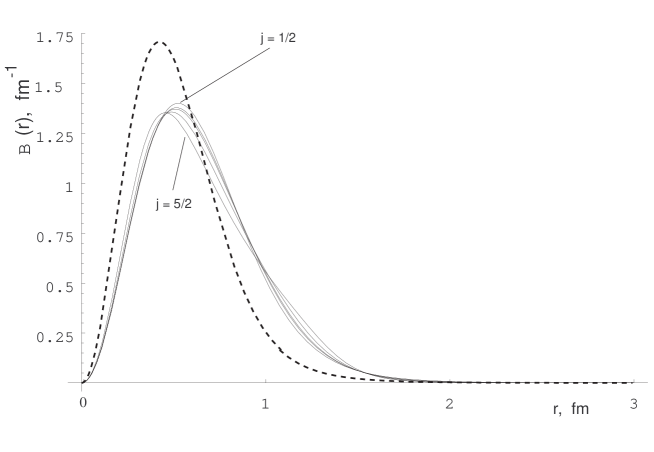
Figure III.1. Baryon charge density distribution. Dashed line denotes classical chiral angle distribution, with parameters $e=5.45;\quad f_{\pi}=64.5$ MeV taken from Ref. [8]. Quantum chiral angle distributions for various $j$ values are plotted with solid lines.

Rotating soliton generates isoscalar magnetic moment associated with current density (III.III.3.10). The matrix elements of the third component of the isoscalar magnetic momentum operator have the form [2]

$$\begin{split}\genfrac{\langle}{|}{0.0pt}{}{\ell}{m_{i},m_{s}}\bigl{[}\hat{\mu}_{I=0}\bigr{]}_{3}\genfrac{|}{\rangle}{0.0pt}{}{\ell}{m_{i},m_{s}}=&\genfrac{\langle}{|}{0.0pt}{}{\ell}{m_{i},m_{s}}\frac{1}{2}\int\mathrm{d}^{3}\mathbf{x}r\bigl{[}\bar{}\mathbf{x}\times\ \hat{\mskip-3.0mu\mskip-3.0mu\mskip-3.0mu\mathscr{B}}\bigr{]}_{0}\genfrac{|}{\rangle}{0.0pt}{}{\ell}{m_{i},m_{s}}\\ =&\frac{e}{f_{\pi}}\frac{\bigl{(}\ell(\ell+1)\bigr{)}^{1/2}}{3\tilde{a}}\bigl{\langle}\tilde{r}_{I=0}^{2}\bigr{\rangle}\Bigl{[}\begin{matrix}\ell&1&\ell\\ m_{s}&0&m_{s}\end{matrix}\Bigr{]},\end{split}$$ (III.III.3.11)

where the isoscalar electric mean square radius is given as

$$\bigl{\langle}r_{E,I=0}^{2}\bigr{\rangle}=\frac{1}{e^{2}f^{2}_{\pi}}\bigl{\langle}\tilde{r}_{E,I=0}^{2}\bigr{\rangle};\qquad\bigl{\langle}\tilde{r}_{E,I=0}^{2}\bigr{\rangle}=-\frac{2}{\pi}\int\tilde{r}^{2}F^{\prime}(\tilde{r})\sin^{2}F(\tilde{r})\mathrm{d}\tilde{r}.$$ (III.III.3.12)

The matrix elements of the third component of the isovector part of magnetic momentum operator that is obtained from the isovector current (III.III.3.7) have the form [2]

$$\begin{split}\genfrac{\langle}{|}{0.0pt}{}{\ell}{m_{i},m_{s}}\bigl{[}\hat{\mu}_{I=1}\bigr{]}_{3}\genfrac{|}{\rangle}{0.0pt}{}{\ell}{m_{i},m_{s}}=&\genfrac{\langle}{|}{0.0pt}{}{\ell}{m_{i},m_{s}}\frac{1}{2}\int\mathrm{d}^{3}\mathbf{x}r\bigl{[}\bar{}\mathbf{x}\times\ \hat{\mskip-3.0mu\mskip-3.0mu\mskip-3.0mu\mathscr{V}}^{a=3}\bigr{]}_{0}\genfrac{|}{\rangle}{0.0pt}{}{\ell}{m_{i},m_{s}}\\ =&\biggl{(}\frac{\tilde{a}}{e^{3}\,f_{\pi}}+\frac{e}{f_{\pi}}\frac{8\pi}{3\tilde{a}^{2}}\int\mathrm{d}\tilde{r}\tilde{r}^{2}\sin^{4}F\Bigl{(}1-\frac{\ell(\ell+1)}{3}-\frac{d_{2}}{2\cdot 5}\\ &+\frac{(-1)^{2\ell}}{2}{\Bigl{(}{\textstyle\frac{5\ell(\ell+1)(2\ell-1)(2\ell+1)(2\ell+3)}{2\cdot 3}\Bigr{)}}^{\frac{1}{2}}}\Bigl{\{}\begin{matrix}1&2&1\\ \ell&\ell&\ell\end{matrix}\Bigr{\}}\Bigl{)}\biggr{)}\\ &\times\Bigl{[}\begin{matrix}\ell&1&\ell\\ m_{s}&0&m_{s}\end{matrix}\Bigr{]}\Bigl{[}\begin{matrix}\ell&1&\ell\\ m_{i}&0&m_{i}\end{matrix}\Bigr{]},\end{split}$$ (III.III.3.13)

where the symbol in the curly brackets is a $6j$ coefficient [82].

From (III.III.3.11) and (III.III.3.13) proton and neutron magnetic moments measured in nuclear magnetons can be extracted using relations

$$\mu_{p}= \frac{1}{2}\Bigl{(}{\scriptstyle\genfrac{\langle}{|}{0.0pt}{}{1/2}{1/2,1/2}[\hat{\mu}_{I=0}]_{3}\genfrac{|}{\rangle}{0.0pt}{}{1/2}{1/2,1/2}+\genfrac{\langle}{|}{0.0pt}{}{1/2}{1/2,1/2}[\hat{\mu}_{I=1}]_{3}\genfrac{|}{\rangle}{0.0pt}{}{1/2}{1/2,1/2}}\Bigr{)},$$ (III.III.3.14a)

$$\mu_{n}= \frac{1}{2}\Bigl{(}{\scriptstyle\genfrac{\langle}{|}{0.0pt}{}{1/2}{-1/2,1/2}[\hat{\mu}_{I=0}]_{3}\genfrac{|}{\rangle}{0.0pt}{}{1/2}{-1/2,1/2}-\genfrac{\langle}{|}{0.0pt}{}{1/2}{-1/2,1/2}[\hat{\mu}_{I=1}]_{3}\genfrac{|}{\rangle}{0.0pt}{}{1/2}{-1/2,1/2}}\Bigr{)}.$$ (III.III.3.14b)

Similar formulas exist for $\Delta_{33}$-resonance magnetic moments

$$\Delta_{33}^{++}= \frac{1}{2}\Bigl{(}{\scriptstyle\genfrac{\langle}{|}{0.0pt}{}{3/2}{3/2,3/2}[\hat{\mu}_{I=0}]_{3}\genfrac{|}{\rangle}{0.0pt}{}{3/2}{3/2,3/2}+\genfrac{\langle}{|}{0.0pt}{}{3/2}{3/2,3/2}[\hat{\mu}_{I=1}]_{3}\genfrac{|}{\rangle}{0.0pt}{}{3/2}{3/2,3/2}}\Bigr{)},$$ (III.III.3.15a)

$$\Delta_{33}^{+\phantom{+}}= \frac{1}{2}\Bigl{(}{\scriptstyle\genfrac{\langle}{|}{0.0pt}{}{3/2}{1/2,3/2}[\hat{\mu}_{I=0}]_{3}\genfrac{|}{\rangle}{0.0pt}{}{3/2}{1/2,3/2}+\genfrac{\langle}{|}{0.0pt}{}{3/2}{1/2,3/2}[\hat{\mu}_{I=1}]_{3}\genfrac{|}{\rangle}{0.0pt}{}{3/2}{1/2,3/2}}\Bigr{)},$$ (III.III.3.15b)

$$\Delta_{33}^{0\phantom{+}}= \frac{1}{2}\Bigl{(}{\scriptstyle\genfrac{\langle}{|}{0.0pt}{}{3/2}{-1/2,3/2}[\hat{\mu}_{I=0}]_{3}\genfrac{|}{\rangle}{0.0pt}{}{3/2}{-1/2,3/2}+\genfrac{\langle}{|}{0.0pt}{}{3/2}{-1/2,3/2}[\hat{\mu}_{I=1}]_{3}\genfrac{|}{\rangle}{0.0pt}{}{3/2}{-1/2,3/2}}\Bigr{)},$$ (III.III.3.15c)

$$\Delta_{33}^{-\phantom{+}}= \frac{1}{2}\Bigl{(}{\scriptstyle\genfrac{\langle}{|}{0.0pt}{}{3/2}{-3/2,3/2}[\hat{\mu}_{I=0}]_{3}\genfrac{|}{\rangle}{0.0pt}{}{3/2}{-3/2,3/2}+\genfrac{\langle}{|}{0.0pt}{}{3/2}{-3/2,3/2}[\hat{\mu}_{I=1}]_{3}\genfrac{|}{\rangle}{0.0pt}{}{3/2}{-3/2,3/2}}\Bigr{)}.$$ (III.III.3.15d)

Relations (III.III.3.14) also allow us to obtain proton and neutron charge distributions, when isoscalar and isovector current densities are used instead of integrated expressions (III.III.3.11) and (III.III.3.13). These distributions are measurable quantities for which semi-empirical formulas exist [123]

$$\rho_{p} =\frac{M^{3}_{D}r^{2}}{2}\exp\bigl{(}-M_{D}r\bigr{)};\qquad M_{D}=0.84~{}\mathrm{GeV},$$ (III.III.3.16a)

$$\rho_{n} =\frac{-\mu_{n}M_{D}^{4}r}{2(5.6M_{D}^{2}-4m_{N}^{2})}\biggl{(}\frac{8m_{N}^{2}\bigl{(}\exp(-M_{D}r)-\exp(-2m_{N}r/\sqrt{5.6})\bigr{)}}{5.6M_{D}^{2}-4m_{N}^{2}}$$

$$\phantom{=\frac{-\mu_{n}M_{D}^{4}r}{2(5.6M_{D}^{2}-4m_{N}^{2})}\biggl{(}}+rM_{D}\exp(-M_{D}r)\biggl{)}.$$ (III.III.3.16b)

Distributions for classical (short-dashed) and quantum chiral angles in various representations (solid lines) are plotted versus semi-empirical distribution (III.III.3.16b) and (III.III.3.16a) (long-dashed line) in Fig. III.2 for proton and in Fig. III.3 for neutron.

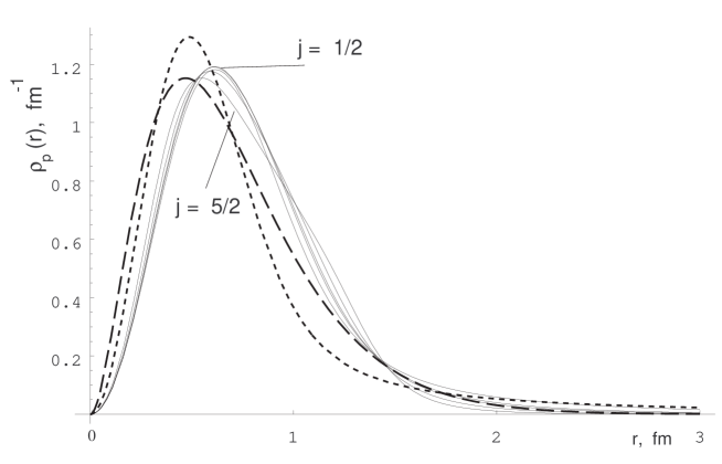
Figure III.2. Proton charge density distribution. Short-dashed line denotes classical chiral angle distribution, with parameters $e=5.45;\quad f_{\pi}=64.5$ MeV from Ref. [8]. Quantum chiral angle distributions for various $j$ values are plotted with solid lines. Long-dashed line denotes semi-empirical charge density distribution [123].

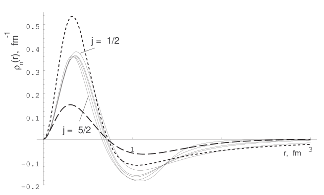
Figure III.3. Neutron charge density distribution. Short-dashed line denotes classical chiral angle distribution, with parameters $e=5.45;\quad f_{\pi}=64.5$ MeV from Ref. [8]. Quantum chiral angle distributions for various $j$ values are plotted with solid lines. Long-dashed line denotes semi-empirical charge density distribution [123].

The neutron distribution peak value ($\sim 0.5$) in classical Skyrme model is known to be too large when compared with the empirical value ($0.2-0.3$). Our results for quantum chiral angle show significant improvement in neutron charge density distribution, which only weakly depends on the representation used. Note also that measurement indicates much faster distribution fall in the asymptotic region even when compared with semi-empirical formula [123]. Speed up of quantum chiral soliton distribution fall thus is also a step in right direction. For experimental distributions we refer to [123] and references therein. The axial coupling $g_{A}$ measures the spin-isospin correlation in the nucleon and is defined as the expectation value of the axial current $A^{a}_{\mu}$ in a nucleon state at zero momentum transfer [53]. Comparison of the Fourier transform of the axial current density (III.III.3.8) with the usual phenomenological expression for the axial-vector current leads to the axial-vector coupling constant expression. From the axial current density (III.III.3.8) we obtain the axial coupling constant $g_{A}$ of the nucleon as [2]

$$g_{A}= -3\genfrac{\langle}{|}{0.0pt}{}{1/2}{1/2,1/2}\int\mathrm{d}^{3}\mathbf{x}\ \ \hat{\mskip-3.0mu\mskip-3.0mu\mskip-3.0mu\mskip-3.0mu\mathscr{A}}_{0}^{1}\genfrac{|}{\rangle}{0.0pt}{}{1/2}{-1/2,1/2}$$

$$= -\frac{1}{e^{2}}\tilde{g}_{1}(F)-\frac{\pi^{2}e^{2}}{3\tilde{a}^{2}(F)}\bigl{\langle}\tilde{r}_{E,I=0}^{2}\bigr{\rangle},$$ (III.III.3.17)

where

$$\tilde{g}_{1}(F)= \frac{4\pi}{3}\int\mathrm{d}\tilde{r}\Bigl{(}\tilde{r}^{2}F^{\prime}+\tilde{r}\sin 2F+\tilde{r}F^{\prime 2}\sin 2F+2F^{\prime}\sin^{2}F+\frac{\sin^{2}\mskip-3.0muF}{\tilde{r}}\sin 2F\Bigr{)}.$$ (III.III.3.18)

All versions of the topological soliton model lead to underprediction of $g_{A}$ compared to the empirical value of $1.26$. In the simple Skyrme model with a pion mass term [132] the predicted value for $g_{A}$ was only $0.65$. By readjusting the parameters so as to fit empirical values for $f_{\pi}$ and $\pi NN$ coupling constant the value is somewhat increased (to $0.82$). In the vector-meson-stabilised model [124] the values range between $0.88$ and $0.99$, depending on the details of the model, but remains below unity [125]. We shall see (see Tables of numerical results) that axial coupling constant $g_{A}$ strongly depends (always grows with increasing dimension of representation) on the representation employed. In self-consistent quantum formalism in higher representations ($j>1/2$) $g_{A}$ is always above unity even for small ($\sim 0.5$ MeV) parameter $f_{\pi}$ values.

III.3.4. Radii

In addition to electric mean square radius (III.III.3.12) the following three mean square radii are used: electric isovector, isoscalar magnetic, isovector magnetic. Below we give definitions for all of them following Ref. [8].

For nucleons the isovector (electric) charge mean square radius becomes

$$\left\langle r_{E,I=1}^{2}\right\rangle =\frac{1}{e^{2}f_{\pi}^{2}}\left\langle\tilde{r}_{E,I=1}^{2}\right\rangle$$

$$=\frac{1}{e^{2}f_{\pi}^{2}}\frac{\int\mathrm{d}\tilde{r}\tilde{r}^{4}\sin^{2}\mskip-3.0muF\Bigl{(}1+F^{\prime 2}+\frac{\sin^{2}\mskip-3.0muF}{\tilde{r}}\Bigr{)}}{\int\mathrm{d}\tilde{r}\tilde{r}^{2}\sin^{2}\mskip-3.0muF\Bigr{(}1+F^{\prime 2}+\frac{\sin^{2}\mskip-3.0muF}{\tilde{r}}\Bigr{)}}.$$ (III.III.3.19)

The isoscalar magnetic mean square radius is expressed as

$$\left\langle r_{M,I=0}^{2}\right\rangle =\frac{1}{e^{2}f_{\pi}^{2}}\left\langle\tilde{r}_{M,I=0}^{2}\right\rangle$$

$$=-\frac{1}{e^{2}f_{\pi}^{2}}\frac{2}{\pi}\frac{\int\mathrm{d}\tilde{r}\tilde{r}^{4}F^{\prime}\sin^{2}\mskip-3.0muF}{\int\mathrm{d}\tilde{r}\tilde{r}^{2}F^{\prime}\sin^{2}\mskip-3.0muF},$$ (III.III.3.20)

and the isovector magnetic mean square radius takes the form

$$\left\langle r_{M,I=1}^{2}\right\rangle =\frac{1}{e^{2}f_{\pi}^{2}}\left\langle\tilde{r}_{M,I=1}^{2}\right\rangle$$

$$=\frac{1}{e^{2}f_{\pi}^{2}}\frac{\int\mathrm{d}\tilde{r}\tilde{r}^{4}\sin^{2}\mskip-3.0muF\Bigl{(}1+F^{\prime 2}+\frac{\sin^{2}\mskip-3.0muF}{\tilde{r}}+\frac{e^{2}\sin^{2}\mskip-3.0muF}{\tilde{a}^{2}(F)}\bigl{(}\frac{3}{4}-\frac{d_{2}}{10}\bigr{)}\Bigr{)}}{\int\mathrm{d}\tilde{r}\tilde{r}^{2}\sin^{2}\mskip-3.0muF\Bigl{(}1+F^{\prime 2}+\frac{\sin^{2}\mskip-3.0muF}{\tilde{r}}+\frac{e^{2}\sin^{2}\mskip-3.0muF}{\tilde{a}^{2}(F)}\bigl{(}\frac{3}{4}-\frac{d_{2}}{10}\bigr{)}\Bigr{)}}.$$ (III.III.3.21)

All these radii can be measured experimentally.

III.4. The static properties of the nucleon and $\Delta_{33}$-resonance in classical chiral angle approach

The normalized state vector with equal fixed spin and isospin $\ell$ are to be identified with nucleons ($\ell=\frac{1}{2}$) and $\Delta_{33}$ resonances ($\ell=\frac{3}{2}$). Before we proceed with the self-consistent quantum case it is worth to examine quantum formulae with classical chiral angle solution (see Fig. II.2). We restrict this numerical analysis to irreducible representations only. Clearly, numerical values for reducible representations lie in the range between minimal and maximal $j$ values of which reducible representation is constructed.

Table III.1. The predicted static baryon observables as obtained with the quantum Skyrme model for representations of different dimension. The first column (ANW) are the predictions for the classical Skyrme model given in Ref. [8]. Classical chiral angle function (taken from ANW column) has been used for evaluation of integrals. The empirical results [127] are listed in the last column.

	ANW	$\mathbf{j=1/2}$	$\mathbf{j=1}$	$\mathbf{j=3/2}$	$\mathbf{j=2}$	$\mathbf{j=5/2}$	Expt.
$m_{N}$	Input	Input	Input	Input	Input	Input	$\hphantom{0}939$ MeV
$m_{\Delta}$	Input	Input	Input	Input	Input	Input	$1232$ MeV
$f_{\pi}$	$\hphantom{0}64.5$	$\hphantom{0}72.1$	$\hphantom{0}76.4$	$\hphantom{0}82.2$	$\hphantom{0}89.4$	$\hphantom{0}98.0$	$\hphantom{00}93$ MeV
$e$	$\hphantom{00}5.45$	$\hphantom{00}5.23$	$\hphantom{00}5.15$	$\hphantom{00}5.03$	$\hphantom{00}4.89$	$\hphantom{00}4.74$
$r_{0}$	$\hphantom{00}0.59$	$\hphantom{00}0.55$	$\hphantom{00}0.53$	$\hphantom{00}0.51$	$\hphantom{00}0.48$	$\hphantom{00}0.45$	$\hphantom{000}0.72$ fm
$\mu_{p}$	$\hphantom{00}1.87$	$\hphantom{00}1.90$	$\hphantom{00}1.84$	$\hphantom{00}1.78$	$\hphantom{00}1.71$	$\hphantom{00}1.64$	$\hphantom{000}2.79$
$\mu_{n}$	$-1.31$	$-1.42$	$-1.40$	$-1.37$	$-1.35$	$-1.33$	$\hphantom{0}-1.91$
$g_{A}$	$\hphantom{00}0.61$	$\hphantom{00}0.62$	$\hphantom{00}0.65$	$\hphantom{00}0.68$	$\hphantom{00}0.73$	$\hphantom{00}0.78$	$\hphantom{000}1.26$
$\mu_{\Delta^{++}}$		$\hphantom{00}3.70$	$\hphantom{m}3.58$	$\hphantom{m}3.44$	$\hphantom{m}3.29$	$\hphantom{m}3.15$	$3.7-7.5$
$\mu_{\Delta^{+}}$		$\hphantom{m}1.71$	$\hphantom{m}1.64$	$\hphantom{m}1.55$	$\hphantom{m}1.46$	$\hphantom{m}1.37$	$\hphantom{000}?$
$\mu_{\Delta^{0}}$		$-0.28$	$-0.31$	$-0.34$	$-0.38$	$-0.42$	$\hphantom{000}?$
$\mu_{\Delta^{-}}$		$-2.27$	$-2.25$	$-2.23$	$-2.21$	$-2.20$	$\hphantom{000}?$

Classical chiral angle is obtained by solving the classical equation of motion (II.II.1.30) (with appropriate boundary conditions) that is given by the requirement that the classical mass (III.III.2.41) be stationary. Asymptotic behaviour when $\tilde{r}\rightarrow\infty$ of classical solution can be easily found from asymptotic equation

$$F^{\prime\prime}(\tilde{r})+\frac{2}{\tilde{r}}F^{\prime}(\tilde{r})-\frac{2}{\tilde{r}^{2}}F(\tilde{r})=0.$$ (III.III.4.1)

Physical solution (satisfying $F(\tilde{r}\rightarrow\infty)=0$) of (III.III.4.1) is

$$F(\tilde{r}\rightarrow\infty)=\frac{k}{\tilde{r}^{2}};\qquad k=\text{const,}$$ (III.III.4.2)

where $k$ is determined by derivative continuity requirement and equation (II.II.1.30) solution value at $\tilde{r}=0$: $F(0)=\pi$. Classical equations of motion can be solved, for example, in the following way.

1. Fix a merge point $\tilde{r}_{0}$ (it is assumed that asymptotic (III.III.4.2) gives a good approximation to the solution at that point) and from (III.III.4.2) calculate function $F(\tilde{r}_{0})$ and its derivative $F^{\prime}(\tilde{r}_{0})$ values at that point.

2. Choose arbitrary $k$ and start standard differential equation iteration procedure until point $\tilde{r}=0$ is reached.

3. If $F(0)\neq\pi$ adjust $k$ value, recalculate $F(\tilde{r}_{0})$ and $F^{\prime}(\tilde{r}_{0})$ values and start differential equation iteration procedure again until $F(0)=\pi$ to the required precision is achieved.

Table III.2. The predicted static baryon observables for representations of different dimension with fixed empirical values for the isoscalar radius and the axial coupling constant.

	$\mathbf{j=1/2}$	$\mathbf{j=1}$	$\mathbf{j=2}$	$\mathbf{j=3}$	$\mathbf{j=4}$	$\mathbf{j=9/2}$	$\mathbf{j=7}$
$m_{N}$	$1434$	$1402$	$1300$	$1147$	$\hphantom{0}942$	$\hphantom{0}821$	$\hphantom{00}23$
$m_{\Delta}$	$1552$	$1520$	$1418$	$1265$	$1060$	$\hphantom{0}939$	$\hphantom{0}141$
$f_{\pi}$	$\hphantom{0}76.2$	$\hphantom{0}76.2$	$\hphantom{0}76.2$	$\hphantom{0}76.2$	$\hphantom{0}76.2$	$\hphantom{0}76.2$	$\hphantom{0}76.2$
$e$	$\hphantom{00}3.81$	$\hphantom{00}3.81$	$\hphantom{00}3.81$	$\hphantom{00}3.81$	$\hphantom{00}3.81$	$\hphantom{00}3.81$	$\hphantom{00}3.81$
$r_{0}$	Input	Input	Input	Input	Input	Input	Input
$\mu_{p}$	$\hphantom{00}4.18$	$\hphantom{00}4.15$	$\hphantom{00}4.07$	$\hphantom{00}3.96$	$\hphantom{00}3.80$	$\hphantom{00}3.70$	$\hphantom{00}3.08$
$\mu_{n}$	$-3.85$	$-3.83$	$-3.75$	$-3.63$	$-3.47$	$-3.38$	$-2.76$
$g_{A}$	Input	Input	Input	Input	Input	Input	Input
$\mu_{\Delta^{++}}$	$\hphantom{00}7.72$	$\hphantom{00}7.67$	$\hphantom{00}7.53$	$\hphantom{00}7.32$	$\hphantom{00}7.03$	$\hphantom{00}6.86$	$\hphantom{00}5.75$
$\mu_{\Delta^{+}}$	$\hphantom{00}2.90$	$\hphantom{00}2.89$	$\hphantom{00}2.84$	$\hphantom{00}2.77$	$\hphantom{00}2.67$	$\hphantom{00}2.61$	$\hphantom{00}2.24$
$\mu_{\Delta^{0}}$	$-1.92$	$-1.90$	$-1.85$	$-1.78$	$-1.69$	$-1.63$	$-1.26$
$\mu_{\Delta^{-}}$	$-6.73$	$-6.69$	$-6.55$	$-6.33$	$-6.05$	$-5.88$	$-4.77$

When classical solution is obtained, the corresponding values for the Lagrangian parameters can be extracted from equations (III.III.4.3) or (III.III.3.17) and (III.III.3.12), or from any of two combinations of them. As in Ref. [8], we determine the two parameters in the Lagrangian (III.III.2.39) so that nucleon and $\Delta_{33}$-resonance masses take their empirical values. The expressions for these masses are then given by (III.III.2.52)

$$m_{N} =\frac{f_{\pi}}{e}\tilde{M}(F)+e^{3}f_{\pi}\Delta\tilde{M}_{j}(F)+\frac{3e^{3}f_{\pi}}{2\cdot 4\tilde{a}(F)},$$ (III.III.4.3a)

$$m_{\Delta} =\frac{f_{\pi}}{e}\tilde{M}(F)+e^{3}f_{\pi}\Delta\tilde{M}_{j}(F)+\frac{15e^{3}f_{\pi}}{2\cdot 4\tilde{a}(F)}.$$ (III.III.4.3b)

In the evaluation of these two masses numerically we employ the classical chiral angle $F(r)$, the shape of which is shown in Fig. II.2.

In Table III.1 we include the predicted values for static nucleon properties [2], as well as the original predictions obtained in Ref. [8] for the classical Skyrme model. For larger values of $j$ the quantum corrections become increasingly important. The key qualitative feature is that the quantum mass correction $\Delta M_{j}(F)$ is negative, with a magnitude that grows with the dimension of the representation. Therefore it becomes possible to reproduce the empirical nucleon and $\Delta_{33}$-resonance mass values with increasingly realistic values of the pion decay constant $f_{\pi}$ as the dimension increases. This reaches its empirical value for a representation $j=5/2$ of dimension 6. There is an accompanying — if less significant — improvement of the numerical value for the axial coupling constant $g_{A}$.

In the case of the isoscalar radius $r_{0}$ (Tables III.1 and III.2) of the baryon, there is, however, no reduction of the difference between the predicted and the empirical value with increasing dimension of the representation. The same is true for the magnetic moments. The predicted value for the ratio of the proton and neutron magnetic moments actually deteriorates slowly with increasing dimension of the representation. In Table III.2 we show the representation dependence of the observables for the case where the parameters are determined by matching the empirical values of isoscalar radius $r_{E,I=0}$ and the axial coupling constant $g_{A}$. Because the expressions (III.III.3.17) and (III.III.3.12) are independent of the dimension of the representation, parameters $f_{\pi}$ and $e$ remain constant. The best agreement with the empirical values of the static properties of baryons in this case are obtained with the representation $j=4$.

We see that when the Skyrme model is treated consistently quantum mechanically ab initio the dimension of the representation becomes a significant additional model parameter [1, 3]. By choosing two parameters of the model so as to match the empirical nucleon and $\Delta_{33}$-resonance masses it becomes possible to obtain a value for the pion decay constant, which is very close to the empirical value ($89.4$ MeV vs. $93$ MeV). There was, however, no comparable gain in quality of the predictions for the baryon magnetic moments, which deteriorated slowly with increasing dimension of the representation. The value of axial coupling constant does on the other hand improve with increasing dimension, but stay below unity for representations of reasonably low dimension.

When parameters of the model are chosen to match isoscalar radius and axial coupling constant, the parameters $f_{\pi}$ and $e$ are constants and nucleon and $\Delta_{33}$-resonance observables depend only on the dimension of the representation. In contrast to the first match, the magnetic moments improved with increasing dimension of the representation. Note that the treatment used here for the quantum skyrmion breaks down when the dimension of the representation grows so large that the negative quantum mass correction $\Delta M_{j}$ becomes of the same order of magnitude as or larger than the classical skyrmion mass. As shown in Table III.2 the numerical value of the quantum mass correction $\Delta M_{j}(F)$ (III.III.2.42) is of the order of $55$ MeV in the fundamental representation, but it rapidly increases in magnitude as the dimension of the representation grows. For a representation of dimension $9$ $(j=4)$ it is large enough to cancel the $\sim 500$ MeV overprediction of the nucleon mass that is obtained when the empirical value for the pion decay constant is employed in the classical Skyrme model. For $j=15/2$ the quantum mass correction exceeds the skyrmion mass and baryon masses become negative. After these comments we skip directly to quantum self-consistent treatment.

III.5. Self-consistent quantum formalism

Minimization of the expression for the classical mass $M(F)$ (III.III.2.41) leads to the conventional differential equation for the chiral angle (II.II.1.30) according to which $F(\tilde{r})$ falls as $1/{\tilde{r}^{2}}$ at large distances. The behaviour is typical for long-range interaction and, therefore, implies zero pion mass. This is inconsistent with strong interaction properties, which is known to be short-range and according to Yukawa [129] imply

$$\boldsymbol{\pi}(r\rightarrow\infty)=-\frac{{\scriptscriptstyle\text{int. const}}}{r}\mathrm{e}^{-\tilde{m}r};\qquad\tilde{m}=\frac{mc}{\hbar},$$ (III.III.5.1)

pion field $\boldsymbol{\pi}(r)$ fall and, therefore, finite pion mass. T.H.R. Skyrme in his 1962 work [6] wrote "These mesons have zero mass, ultimately on account of the full rotational symmetry of the Lagrangian (II.II.1.6). This symmetry is, however, destroyed by the boundary condition $\mathbf{U}(\infty)=\mathbf{1}$, and we believe that the mass may arise as a self consistent quantal effect." Thus, T.H.R. Skyrme noted that chiral group $SU(2)_{L}\otimes SU(2)_{R}$ is spontaneously broken by choosing vacuum state $\mathbf{U}(\infty)=\mathbf{1}$ to the subgroup $\operatorname{diag}\bigl{(}SU(2)_{L}\otimes SU(2)_{R}\bigr{)}\sim SU(2)_{I}$. According to the recent point of view just the spontaneous breakdown of chiral symmetry implies massless pions. In other words, pion is massless provided that the axial current is perfectly conserved. Because a pion is massive, we expect that axial symmetry should be an approximate symmetry and that the axial current should be only approximately (partially) conserved.

In the semiclassical approach the quantum mass term $\Delta{M}_{\Sigma_{j}}$ is absent from the mass expression (III.III.2.52). The absence of negative $\Delta{M}_{\Sigma_{j}}$ correction has the consequence that variation of the truncated quantum mass expression yields no stable solution [34, 130]. The semiclassical approach describes the skyrmion as a “rotating” rigid body with fixed $F(r)$ [8]. In contrast the variation of the full energy expression (III.III.2.52) that is obtained in the consistent canonical quantization procedure [48] in collective coordinates approach gives stable solutions.

Minimization of the quantum mass expression (III.III.2.52) leads to the following integro-differential equation for the chiral angle $F(\tilde{r})$ in the dimensionless variable $\tilde{r}$:

$$\begin{split}\ &F^{\prime\prime}\biggl{(}-2\tilde{r}^{2}-4\sin^{2}\mskip-3.0muF+\frac{e^{4}\tilde{r}^{2}\sin^{2}\mskip-3.0muF}{15\tilde{a}^{2}}\Bigl{(}80\tilde{a}\Delta\tilde{M}_{\Sigma_{j}}+20\ell(\ell+1)+4d_{1}-8d_{2}\sin^{2}\mskip-3.0muF\Bigr{)}\biggr{)}\\ +&F^{\prime 2}\biggl{(}-2\sin 2F+\frac{e^{4}\tilde{r}^{2}\sin 2F}{15\tilde{a}^{2}}\Bigl{(}40\tilde{a}\Delta\tilde{M}_{\Sigma_{j}}+10\ell(\ell+1)+2d_{1}-8d_{2}\sin^{2}\mskip-3.0muF\Bigr{)}\biggr{)}\\ +&F^{\prime}\biggl{(}-4\tilde{r}+\frac{e^{4}\tilde{r}\sin^{2}\mskip-3.0muF}{15\tilde{a}^{2}}\Bigl{(}160\tilde{a}\Delta\tilde{M}_{\Sigma_{j}}+40\ell(\ell+1)+8d_{1}-16d_{2}\sin^{2}\mskip-3.0muF\Bigr{)}\biggr{)}\\ +&\sin 2F\biggl{(}2+2\frac{\sin^{2}\mskip-3.0muF}{\tilde{r}^{2}}-\frac{e^{4}}{15\tilde{a}^{2}}\Bigl{(}\bigl{(}40\tilde{a}\Delta\tilde{M}_{\Sigma_{j}}+10\ell(\ell+1)\bigr{)}\bigl{(}\tilde{r}^{2}+2\sin^{2}\mskip-3.0muF\bigr{)}+15\tilde{r}^{2}\\ \ &\phantom{\sin 2F\biggl{(}2+2\frac{\sin^{2}\mskip-3.0muF}{\tilde{r}^{2}}-\frac{e^{4}}{15\tilde{a}^{2}}\Bigl{(}}+4d_{3}\sin^{2}\mskip-3.0muF+8d_{2}\tilde{r}^{2}\sin^{2}\mskip-3.0muF\Bigr{)}\biggr{)}=0,\end{split}$$ (III.III.5.2)

with the usual boundary conditions $F(0)=\pi$ and $F(\infty)=0$. The state dependence of this equation is a direct consequence of the fact that quantization preceded variation (cf. Ref. [131]). Contrary to the classical equation (II.II.1.30) quantum chiral angle equation (III.III.5.2) depends on the parameter $e$. This, however, is not an unusual result: quantization of breathing modes [36, 37] also leads to parameter $e$ dependent equations.

At large distances this equation reduces to the asymptotic form

$$\tilde{r}^{2}F^{\prime\prime}+2\tilde{r}F^{\prime}-\bigl{(}2+\tilde{m}_{\pi}^{2}\tilde{r}^{2}\bigr{)}F=0,$$ (III.III.5.3)

where the quantity $\tilde{m}_{\pi}^{2}$ is defined as

$$\tilde{m}_{\pi}^{2}=-\frac{e^{4}}{3\tilde{a}(F)}\Bigl{(}8\Delta\tilde{M}_{\Sigma_{j}}(F)+\frac{2\ell(\ell+1)+3}{\tilde{a}(F)}\Bigr{)},$$ (III.III.5.4)

and the corresponding asymptotic solution takes the form

$$F(\tilde{r})=k\Bigl{(}\frac{\tilde{m}_{\pi}}{\tilde{r}}+\frac{1}{\tilde{r}^{2}}\Bigr{)}\mathrm{e}^{-\tilde{m}_{\pi}\tilde{r}};\qquad k=\text{const}.$$ (III.III.5.5)

The requirement of stability of the quantum skyrmion is that the integrals (III.III.2.8), (III.III.2.41) and (III.III.2.42) converge. This requirement is satisfied only if $\tilde{m}_{\pi}^{2}>0$. For that the presence of the negative quantum correction $\Delta M_{\Sigma_{j}}(F)$ is necessary. The absence of this term leads to the instability of the skyrmion in the semiclassical approach [34]. Note that in the quantum treatment the chiral angle possesses [48] the asymptotic Yukawa behaviour (III.III.5.5). The positive quantity $m_{\pi}=ef_{\pi}\tilde{m}_{\pi}$, therefore, can be interpreted as an effective mass for the pion field.

It is known that in classical Skyrme model 3-divergence of axial current density component $\mathscr{A}^{a}(\mathbf{x})$ gives the differential equation (II.II.1.30) for chiral angle [35]. "Therefore, in this chiral-symmetric theory the conservation of axial-vector current is, in fact, the equation of motion, i.e. the Euler-Lagrange equation for the rotated pion field $\pi_{i}$" [131]. Let’s assume that in quantum theory axial symmetry is broken and the matrix element of the divergence of axial current is proportional to pion mass (PCAC relation)

$$\genfrac{\langle}{|}{0.0pt}{}{\ell}{m_{i},m_{s}}\nabla^{b}\ \ \hat{\mskip-3.0mu\mskip-3.0mu\mskip-3.0mu\mskip-3.0mu\mathscr{A}}_{b}^{a}\genfrac{|}{\rangle}{0.0pt}{}{\ell}{m_{i},m_{s}}=f_{\pi}^{2}m_{\pi}^{2}F(r).$$ (III.III.5.6)

As a consequence we get the same asymptotic equation (III.III.5.3), when $r\rightarrow\infty$. This result supports the interpretation of $m_{\pi}$ as the effective pion mass.

Note also that the finite pion mass in the Skyrme model is usually introduced by adding an explicit term [36, 48, 132]

$$\mathscr{L}_{m_{\pi}}=\frac{1}{4}m_{\pi{\scriptscriptstyle(exp)}}^{2}f_{\pi}^{2}\operatorname{Tr}\{\mathbf{U}+\mathbf{U}^{\dagger}-2\},$$ (III.III.5.7)

in the Lagrangian density (II.II.1.6), and, therefore, the Lagrangian (II.II.1.6) chiral symmetry becomes explicitly broken even in classical limit.

Positivity of the pion mass (III.III.5.4) can obviously only be achieved for states with sufficiently small values of spin $\ell$. This implies that the spectrum of states with equal spin and isospin will necessarily terminate at some finite value of the spin quantum number $\ell$. The termination point depends on parameters $e$ and $j$ values. When spin $\ell$ value increases, the upper $e$ value for which stable soliton solution exist always decreases (for the same representation $j$). As the negative quantum mass correction $\Delta M_{\Sigma_{j}}$ in the expression (III.III.2.42) grows in magnitude with the dimension of the representation, it is always possible to find a representation in which the nucleon and the $\Delta_{33}$-resonance are the only stable particles, as required by experiment.

Integro-differential equation (III.III.5.2) can be attacked in the following way.

1. Using chiral classical angle Fig. II.2 and any pair of empirical baryon observables, for example, nucleon mass (III.III.4.3a) and isoscalar radius (III.III.3.12) we fit two model parameters $f_{\pi}$ and $e$ and calculate all required integrals in the quantum equation (III.III.5.2), namely, (III.III.2.41), (III.III.2.8), (III.III.2.42), (III.III.5.4).

2. Using known asymptotic solution (III.III.5.5) (and its derivative) one can adopt simple differential equation solution procedure described in Sec. III.4 and find the first quantum solution $F_{1}(\tilde{r})$ and the constant $k_{1}$.

3. This quantum solution $F_{1}(\tilde{r})$ now can be subsequently used to recalculate $f_{\pi},e$ and integrals (III.III.2.41), (III.III.2.8), (III.III.2.42), (III.III.5.4). Then again procedure described in item 2 can be used to get the solution $F_{2}(\tilde{r})$ and constant $k_{2}$.

4. This procedure can be iterated until convergent solution and parameters $f_{\pi},e$ as well as stable values of $M(F),\Delta M_{\Sigma_{j}}(F),a(F),m_{\pi}(F)$ are obtained. The self-consistent set then can be used to calculate numerous phenomenologically interesting quantities.

Quantum chiral angle solutions with model parameters determined from nucleon mass (III.III.4.3a) and isoscalar radius (III.III.3.12) are shown in Fig. III.4. If one succeeds in initial guess, then it usually takes only $10$–$15$ iterations to get $5$–$6$ fixed digits in all integrals and $f_{\pi},e$ values.

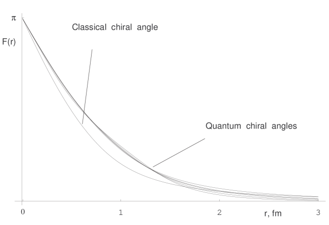
Figure III.4. Quantum chiral angle solution family for nucleon ($\ell=\frac{1}{2}$) in representations $j=\frac{1}{2},1\oplus\frac{1}{2}\oplus\frac{1}{2},1,\frac{3}{2},\frac{5}{2}$ and the classical chiral angle solution as taken from Ref. [8].

For nucleon solutions with spin $\ell=1/2$ exist (in the fundamental representation $j=1/2$) when $0\leq e<7.5$. The largest value of $e$ for which stable solutions are obtained decreases with increasing dimensionality of the representation, and there are no restrictions to the existence of solution from representation $j$ employed. This can be seen from equation (III.III.5.2) itself. Indeed, the formal substitution $e\rightarrow 0$ into (III.III.5.2) yields the classical equation (II.II.1.30), which does have a solution.

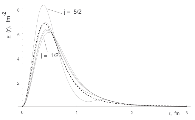
Figure III.5. Family of nucleon mass densities in representations $j=\frac{1}{2},1\oplus\frac{1}{2}\oplus\frac{1}{2},1,\frac{3}{2},\frac{5}{2}$ (model parameters being calculated from empirical nucleon mass (III.III.4.3a) and isoscalar radius (III.III.3.12)).

For illustration (see Fig. III.5) we also provide nucleon mass densities (Hamiltonian densities (III.III.2.52)) for quantum chiral angles in Fig. III.4 and detailed contributions of classical soliton masses, rotation energies and quantum mass corrections for two of them ($j=\frac{1}{2}$ and $j=\frac{5}{2}$) in Fig. III.6

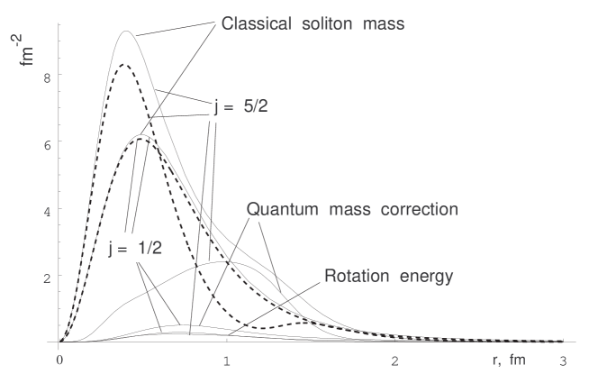
Figure III.6. Detailed contributions of classical soliton masses, rotation energies and quantum mass corrections for nucleon in representations $j=\frac{1}{2}$ and $j=\frac{5}{2}$ (model parameters being calculated from empirical nucleon mass (III.III.4.3a) and isoscalar radius (III.III.3.12)).

A remark is given to the $\sigma$ model without the Skyrme term (this corresponds to the limit $e\rightarrow\infty$ in (II.II.1.6)). Although the quantum correction $\Delta M_{\Sigma_{j}}$ plays a role in stabilization of soliton, one cannot obtain "quantum" rotating chiral soliton without the Skyrme term as stabilizer [133]. Applying higher representations also cannot help in obtaining this stability [134]. This is consistent with Derrick theorem [57]. For $\Delta_{33}$-resonances $(\ell=3/2)$ there are no stable solutions in the fundamental ($j=1/2$) representation, nor in the representation $j=1$. In the representations $j=3/2$ and $j=2$ there are only stable soliton solutions for baryons with spin $\ell=1/2$ and $\ell=3/2$. A dimension with $j=5/2$ allows solitons with $\ell=1/2,\ 3/2$ and $5/2$, and, therefore, appears to be empirically contraindicated. The numerical results for nucleons with fixed empirical values for isoscalar radius and mass are shown in Table A.2 in Appendix A. For the irreducible representation $j=1$ the proton magnetic moment calculated in this way is within 10% of the empirical value. The calculated values of both the neutron magnetic moment and the axial coupling constant agree with the corresponding empirical values to within 1%. Numerical results for fixed isoscalar radius and axial coupling constant are represented in Table A.3 (Appendix A). For representation $j=1$ nucleon mass and proton magnetic moment agree with experimental values within 10%, neutron magnetic moment within 2%. In Table A.1 and Table A.4 we represent numerical results obtained by fixing $m_{\pi}=138$ MeV and nucleon mass (Table A.1) or isoscalar radius (Table A.4). In these approaches agreement with experimental data is worse. We note, however, that pion field mass used here ($138$ MeV) approximately equals to particles $\pi_{0},\pi_{-},\pi_{+}$ mass. The effective strong interaction field fall can be indirectly estimated from experiments. These measurements correspond to about $150$ MeV effective boson mass, when extracted from Yukawa formula (III.III.5.1).

For parameters $e,f_{\pi}$ fixed from nucleon data, empirical values for $\Delta_{33}$-resonance observables for different representations can be obtained. Results for $e=4.15,\ f_{\pi}=58.5$ MeV (determined by fit to nucleon $m_{N}=939$ MeV and $\langle r^{2}_{E,I=0}\rangle^{1/2}=0.72$ fm and representation $j=1$) are demonstrated in Table B.1 in Appendix B. Results for the same fit of experimental quantities, but in different representations are shown in Table B.2 ($j=\frac{1}{2}$) and Table B.3 ($j=1\oplus\frac{1}{2}\oplus\frac{1}{2}$). Tables B.6, B.7, B.8 represent numerical results with fixed values for $e$ and $f_{\pi}$, which are calculated from nucleon observables $g_{A}$ and $\langle r^{2}_{E,I=0}\rangle^{1/2}$ in representations $j=\frac{1}{2};\quad j=1$ and $j=1\oplus\frac{1}{2}\oplus\frac{1}{2}$, respectively. Tables B.4 and B.5 show similar results for fixed $e,f_{\pi}$ values, extracted from nucleon observables $m_{\pi}$ and $\langle r^{2}_{E,I=0}\rangle^{1/2}$ in representations $j=1$ (Table B.4) and $j=1\oplus\frac{1}{2}\oplus\frac{1}{2}$ (Table B.5).

It is also worth to mention the numerical results for reducible representations $1\otimes\frac{1}{2}\otimes\frac{1}{2}$ for nucleon and $\frac{3}{2}\otimes 1\otimes\frac{1}{2}$ for $\Delta_{33}$-resonance. The representation $\frac{3}{2}\otimes 1\otimes\frac{1}{2}$ is the first one for which the stable soliton solution is obtained for $\ell=3/2$ state. The numerical results in these reducible representations are comparable — if not better — to those of representations $j=1$ (for $\ell=1/2$) and $j=3/2$ (for $\ell=3/2$), respectively. Noting that the SU(3) isomultiplets — octet $(1,1)$ and decuplet $(2,0)$ — (to which nucleon and $\Delta_{33}$-resonance belong, respectively) split, when restricted to SU(2) subgroup, into $1\otimes\frac{1}{2}\otimes\frac{1}{2}\otimes 0$ and $\frac{3}{2}\otimes 1\otimes\frac{1}{2}\otimes 0$, respectively, the following explanation is not improbable: it just can indicate that SU(2) Skyrme model in some way (via representations employed) reveals relevant SU(3) symmetry of strong interactions. If this is indeed the case, then in SU(3) Skyrme model using higher representations ($(1,1)$ and $(2,0)$) one can hope to describe the entire isomultiplets of baryons more successfully. Investigation of SU(3) Skyrme model is required to confirm or reject these considerations.

III.6. Remarks on persisting problems

Despite quite successful generalization of quantum Skyrme model to general representation of SU(2) group a few problems still persist. First of all we see rather big gap between calculated ($f_{\pi}\sim 60$ MeV, $e\sim 4$) and extracted from experiment ($f_{\pi}=93$ MeV, $e\sim 7.4$) numerical values of model parameters. The problem is inherited from semiclassical calculations [8]. The difference, however, becomes increasingly important, because all other measurable quantities fit to their experimental values much better ($\sim 10\%$, see Appendix A). Thus the question again arises to what extent do these errors of the Skyrme model reflect use of the approximation, and to what extent do they reflect the fact that the Skyrme model is crude approximation to meson physics. The question has been considered by E. Witten [9], who suspected that in the case of semiclassical approximation "the error mainly has the latter origin$\dots$ If the proper meson theory were known, the semiclassical approximation would be equivalent to the $1/N_{c}$ expansion, and I personally suspect the error would be much less than $30$%". Our calculations, if we exclude $f_{\pi},e$ values, which can be considered just as model parameters without referring to its physical content, are in much better agreement with experimental data. However, it should be noted that we obtain these values due to an additional implicit discrete parameter — the group representation. The quantization procedure also differs from the semiclassical approach [8] considered by E. Witten [9]. A problem is also present with the interpretation of representation dependence itself. Despite the quantization method used here is free of ambiguity and is in agreement with principles of modern quantization of constrained systems, it undoubtedly shows representation dependence of measurable quantities. Thus physical interpretation is welcome and we hope that quantum investigation of SU(3) Skyrme model can enlighten this problem.

Concluding statements

The following statements represent the main results of the work in the order of decreasing importance.

• Each of SU(2) representation $j$ yields the different quantum Lagrangian density. As a consequence, theoretical observables depend on representation $j$ which can be treated as a new phenomenological parameter.

• Quantum chiral solitons exist and possess asymptotic behaviour consistent with the massive Yukawa field fall (III.III.5.1). The asymptotic shape and PCAC relation leads to the correct asymptotic equation (III.III.5.3) coinciding with contribution of explicitly broken term (III.III.5.7). This encourages us to suggest that the integral $m_{\pi}$ should be interpreted as an effective pion mass.

• A nucleon and $\Delta_{33}$-resonance are the only stable states for irreducible representations $j=\frac{3}{2}$ and $j=2$. Unphysical tower of states $\ell_{\text{spin}}=\ell_{\text{isospin}}$, which is artifact of the classical and semiclassical Skyrme model is, therefore, terminated by choosing the appropriate SU(2) representations.

• Higher spin ($\ell>1/2$) quantum states are not "spherically symmetric". The Hamiltonian (III.III.2.53) (Lagrangian (III.III.2.40)) density function depends on the polar angle $\vartheta$. Nucleon states are "spherically symmetric" in various representations of $j$, as required.

• Each of the spin-isospin state yields the different range of realizable values of the parameter $e$. A stable quantum self-consistent solution exist:

  • for spin $\ell=\frac{1}{2}$ states in all SU(2) representations,

  • for $\ell=\frac{3}{2}$ spin states starting at least from reducible representation $\scriptscriptstyle\mathbf{\frac{3}{2}\oplus{\scriptstyle 1}\oplus\frac{1}{2}}$.

• A very good agreement with experimental data is obtained for axial coupling constant $g_{A}$ in higher representations of SU(2), the problem being previously unsolved by using various extensions of the model in the fundamental representation of SU(2).

• The basic quantum Skyrme model provides considerable improvements in nucleon magnetic momenta and, especially, in neutron charge density distribution.

The text of PhD thesis can be found at the Website of Institute of Theoretical Physics and Astronomy
 http://www.itpa.lt/baryon

Appendix A Nucleon observables in different representations

.

Table A.1. The predicted static baryon observables for different representations with fixed empirical values for the effective pion mass $m_{\pi}=138$ MeV and nucleon mass $939$ MeV.

$\mathbf{j}$	$\mathbf{1/2}$	$\mathbf{1}$	$\mathbf{3/2}$	$\scriptscriptstyle\mathbf{1\oplus\frac{1}{2}\oplus\frac{1}{2}}$	Expt.
$m_{N}$	Input	Input	Input	Input	$939$ MeV
$f_{\pi}$	68.4	54.9	49.6	57.2	$93$ MeV
$e$	4.97	3.96	3.52	4.15
$\mu_{p}$	1.63	3.20	4.44	2.80	$2.79$
$\mu_{n}$	$-$1.06	$-$2.61	$-$3.85	$-$2.21	$-1.91$
$g_{A}$	0.89	1.43	1.77	1.30	$1.26$
$m_{\pi}$	Input	Input	Input	Input	$138$ MeV
$\sqrt{\langle r^{2}_{E,I=0}\rangle}$	0.54	0.83	1.00	0.77	$0.72$ fm

Table A.2. The predicted static nucleon observables in different representations with fixed empirical values for the isoscalar radius $\langle r^{2}_{E,I=0}\rangle^{1/2}=0.72$ fm and nucleon mass $939$ MeV.

$\mathbf{j}$	$\mathbf{1/2}$	$\mathbf{1}$	$\mathbf{3/2}$	$\mathbf{5/2}$	$\scriptscriptstyle\mathbf{1\oplus\frac{1}{2}\oplus\frac{1}{2}}$	Expt.
$m_{N}$	Input	Input	Input	Input	Input	$939$ MeV
$f_{\pi}$	59.8	58.5	57.7	56.6	58.8	$93$ MeV
$e$	4.46	4.15	3.86	3.41	4.24
$\mu_{p}$	2.60	2.52	2.51	2.52	2.53	$2.79$
$\mu_{n}$	$-$2.01	$-$1.93	$-$1.97	$-$2.05	$-$1.93	$-1.91$
$g_{A}$	1.20	1.25	1.33	1.52	1.23	$1.26$
$m_{\pi}$	79.5	180.	248.	336.	155.	$138$ MeV
$\sqrt{\langle r^{2}_{E,I=0}\rangle}$	Input	Input	Input	Input	Input	$0.72$ fm
$\sqrt{\langle r^{2}_{E,I=1}\rangle}$	1.33	1.03	0.97	0.93	1.07	$0.88$ fm
$\sqrt{\langle r^{2}_{M,I=0}\rangle}$	1.05	1.01	1.00	1.00	1.01	$0.81$ fm
$\sqrt{\langle r^{2}_{M,I=1}\rangle}$	1.32	1.03	0.97	0.93	1.07	$0.80$ fm

Table A.3. The predicted static baryon observables for different representations with fixed empirical values for the isoscalar radius $\langle r^{2}_{E,I=0}\rangle^{1/2}=0.72$ fm and axial coupling constant $g_{A}=1.26$  .

$\mathbf{j}$	$\mathbf{1/2}$	$\mathbf{1}$	$\mathbf{3/2}$	$\mathbf{5/2}$	$\scriptscriptstyle\mathbf{1\oplus\frac{1}{2}\oplus\frac{1}{2}}$	Expt.
$m_{N}$	986.	948.	882.	694.	963.	$939$ MeV
$f_{\pi}$	61.4	58.9	55.7	48.1	59.7	$93$ MeV
$e$	4.37	4.13	3.92	3.56	4.20
$\mu_{p}$	2.70	2.53	2.42	2.05	2.57	$2.79$
$\mu_{n}$	$-$2.14	$-$1.95	$-$1.84	$-$1.51	$-$1.99	$-1.91$
$g_{A}$	Input	Input	Input	Input	Input	$1.26$
$m_{\pi}$	75.8	179.	259.	386.	152.	$138$ MeV
$\sqrt{\langle r^{2}_{E,I=0}\rangle}$	Input	Input	Input	Input	Input	$0.72$ fm
$\sqrt{\langle r^{2}_{E,I=1}\rangle}$	1.36	1.03	0.96	0.92	1.08	$0.88$ fm
$\sqrt{\langle r^{2}_{M,I=0}\rangle}$	1.05	1.01	1.00	1.01	1.01	$0.81$ fm
$\sqrt{\langle r^{2}_{M,I=1}\rangle}$	1.35	1.03	0.96	0.92	1.08	$0.80$ fm

Table A.4. The predicted static baryon observables for different representations with fixed empirical values for the isoscalar radius $\langle r^{2}_{E,I=0}\rangle^{1/2}=0.72$ fm and effective pion mass $m_{\pi}=138$ MeV.

$\mathbf{j}$	$\mathbf{1/2}$	$\mathbf{1}$	$\mathbf{3/2}$	$\mathbf{5/2}$	$\scriptscriptstyle\mathbf{1\oplus\frac{1}{2}\oplus\frac{1}{2}}$	Expt.
$m_{N}$	486.	1264.	1872.	2992.	1069.	$939$ MeV
$f_{\pi}$	41.7	68.8	84.0	106.3	63.1	$93$ MeV
$e$	5.56	3.76	3.12	2.48	4.05
$\mu_{p}$	1.93	3.13	4.35	6.72	2.77	$2.79$
$\mu_{n}$	$-$0.86	$-$2.68	$-$4.04	$-$6.52	$-$2.24	$-1.91$
$g_{A}$	0.60	1.65	2.46	3.94	1.39	$1.26$
$m_{\pi}$	Input	Input	Input	Input	Input	$138$ MeV
$\sqrt{\langle r^{2}_{E,I=0}\rangle}$	Input	Input	Input	Input	Input	$0.72$ fm
$\sqrt{\langle r^{2}_{E,I=1}\rangle}$	1.07	1.12	1.12	1.12	1.11	$0.88$ fm
$\sqrt{\langle r^{2}_{M,I=0}\rangle}$	1.01	1.02	1.02	1.02	1.02	$0.81$ fm
$\sqrt{\langle r^{2}_{M,I=1}\rangle}$	1.05	1.12	1.12	1.13	1.11	$0.80$ fm

Appendix B $\Delta_{33}$-resonance observables in different representations

Table B.1. The predicted static $\Delta_{33}$-resonance observables in different representations with fixed values for the parameters $e=4.15$ and $f_{\pi}=58.5$ MeV (from nucleon observables $m_{N}=939$ MeV, $\langle r^{2}_{E,I=0}\rangle^{1/2}=0.72$ fm, representation $j=1$ in Table A.2).

$\mathbf{j}$	$\scriptscriptstyle\mathbf{\frac{3}{2}\oplus 1\oplus\frac{1}{2}}$	$\mathbf{\frac{3}{2}}$	$\mathbf{2}$	Expt.
$m_{\Delta}$	1055.	1029.	910.	$1232$ MeV
$\mu_{\Delta^{++}}$	7.38	6.40	4.20	$3.7-7.5$
$\mu_{\Delta^{+}}$	3.02	2.73	2.01	?
$\mu_{\Delta^{0}}$	$-$1.33	$-$0.94	$-$0.19	?
$\mu_{\Delta^{-}}$	$-$5.69	$-$4.61	$-$2.38	?
$\sqrt{\langle r^{2}_{E,I=0}\rangle}$	0.91	0.87	0.72	?

Table B.2. The predicted static $\Delta_{33}$-resonance observables for different representations with fixed empirical values for the $e=4.46$ and $f_{\pi}=59.8$ MeV (from nucleon observables $m_{N}=939$ MeV, $\langle r^{2}_{E,I=0}\rangle^{1/2}=0.72$ fm, representation $j=\frac{1}{2}$ in Table A.2).

$\mathbf{j}$	$\scriptscriptstyle\mathbf{\frac{3}{2}\oplus 1\oplus\frac{1}{2}}$	$\mathbf{\frac{3}{2}}$	$\mathbf{2}$	Expt.
$m_{\Delta}$	1008.	974.	809.	$1232$ MeV
$\mu_{\Delta^{++}}$	6.05	5.15	3.00	$3.7-7.5$
$\mu_{\Delta^{+}}$	2.63	2.36	1.63	?
$\mu_{\Delta^{0}}$	$-$0.80	$-$0.43	0.25	?
$\mu_{\Delta^{-}}$	$-$4.23	$-$3.22	$-$1.12	?
$m_{\pi}$	104.	172.	438.	$138$ MeV
$\sqrt{\langle r^{2}_{E,I=0}\rangle}$	0.84	0.79	0.62	?

Table B.3. The predicted static $\Delta_{33}$-resonance observables for different representations with fixed empirical values for the $e=4.24$ and $f_{\pi}=58.8$ MeV (from nucleon observables $m_{N}=939$ MeV, $\langle r^{2}_{E,I=0}\rangle^{1/2}=0.72$ fm, representation $j=1\oplus\frac{1}{2}\oplus\frac{1}{2}$ in Table A.2).

$\mathbf{j}$	$\scriptscriptstyle\mathbf{\frac{3}{2}\oplus 1\oplus\frac{1}{2}}$	$\mathbf{\frac{3}{2}}$	$\mathbf{2}$	Expt.
$m_{\Delta}$	1040.	1012.	881.	$1232$ MeV
$\mu_{\Delta^{++}}$	6.96	6.00	3.82	$3.7-7.5$
$\mu_{\Delta^{+}}$	2.90	2.61	1.89	?
$\mu_{\Delta^{0}}$	$-$1.16	$-$0.78	$-$0.05	?
$\mu_{\Delta^{-}}$	$-$5.23	$-$4.17	$-$1.98	?
$m_{\pi}$	85.5	141.	338.	$138$ MeV
$\sqrt{\langle r^{2}_{E,I=0}\rangle}$	0.89	0.85	0.69	?

Table B.4. The predicted static $\Delta_{33}$-resonance observables for different representations with fixed empirical values for the $e=3.76$ and $f_{\pi}=68.8$ MeV (from nucleon observables $m_{\pi}=138$ MeV, $\langle r^{2}_{E,I=0}\rangle^{1/2}=0.72$ fm, representation $j=1$ in Table A.4).

$\mathbf{j}$	$\scriptscriptstyle\mathbf{\frac{3}{2}\oplus 1\oplus\frac{1}{2}}$	$\mathbf{\frac{3}{2}}$	$\mathbf{2}$	Expt.
$m_{\Delta}$	1360.	1338.	1245.	$1232$ MeV
$\mu_{\Delta^{++}}$	8.14	7.24	5.28	$3.7-7.5$
$\mu_{\Delta^{+}}$	3.14	2.86	2.23	?
$\mu_{\Delta^{0}}$	$-$1.87	$-$1.52	$-$0.83	?
$\mu_{\Delta^{-}}$	$-$6.87	$-$5.89	$-$3.88	?
$m_{\pi}$	65.3	106.5	234.	$138$ MeV
$\sqrt{\langle r^{2}_{E,I=0}\rangle}$	0.84	0.81	0.72	?

Table B.5. The predicted static $\Delta_{33}$-resonance observables for different representations with fixed empirical values for the $e=4.05$ and $f_{\pi}=63.1$ MeV (from nucleon observables $m_{\pi}=138$ MeV, $\langle r^{2}_{E,I=0}\rangle^{1/2}=0.72$ fm, representation $j=1\oplus\frac{1}{2}\oplus\frac{1}{2}$ in Table A.4).

$\mathbf{j}$	$\scriptscriptstyle\mathbf{\frac{3}{2}\oplus 1\oplus\frac{1}{2}}$	$\mathbf{\frac{3}{2}}$	$\mathbf{2}$	Expt.
$m_{\Delta}$	1162.	1137.	1020.	$1232$ MeV
$\mu_{\Delta^{++}}$	7.25	6.32	4.27	$3.7-7.5$
$\mu_{\Delta^{+}}$	2.92	2.65	1.97	?
$\mu_{\Delta^{0}}$	$-$1.40	$-$1.03	$-$0.32	?
$\mu_{\Delta^{-}}$	$-$5.72	$-$4.71	$-$2.62	?
$m_{\pi}$	78.5	129.	297.	$138$ MeV
$\sqrt{\langle r^{2}_{E,I=0}\rangle}$	0.86	0.82	0.70	?

Table B.6. The predicted static $\Delta_{33}$-resonance observables for different representations with fixed empirical values for the $e=4.37$ and $f_{\pi}=61.4$ MeV (from nucleon observables $g_{A}=1.26$, $\langle r^{2}_{E,I=0}\rangle^{1/2}=0.72$ fm, representation $j=\frac{1}{2}$ in Table A.3).

$\mathbf{j}$	$\scriptscriptstyle\mathbf{\frac{3}{2}\oplus 1\oplus\frac{1}{2}}$	$\mathbf{\frac{3}{2}}$	$\mathbf{2}$	Expt.
$m_{\Delta}$	1053.	1021.	865.	$1232$ MeV
$\mu_{\Delta^{++}}$	6.18	5.28	3.19	$3.7-7.5$
$\mu_{\Delta^{+}}$	2.64	2.37	1.67	?
$\mu_{\Delta^{0}}$	$-$0.90	$-$0.54	0.14	?
$\mu_{\Delta^{-}}$	$-$4.44	$-$3.45	$-$1.39	?
$m_{\pi}$	99.7	165.	409.	$138$ MeV
$\sqrt{\langle r^{2}_{E,I=0}\rangle}$	0.83	0.79	0.62	?

Table B.7. The predicted static $\Delta_{33}$-resonance observables for different representations with fixed empirical values for the $e=4.13$ and $f_{\pi}=58.9$ MeV (from nucleon observables $g_{A}=1.26$, $\langle r^{2}_{E,I=0}\rangle^{1/2}=0.72$ fm, representation $j=1$ in Table A.3).

$\mathbf{j}$	$\scriptscriptstyle\mathbf{\frac{3}{2}\oplus 1\oplus\frac{1}{2}}$	$\mathbf{\frac{3}{2}}$	$\mathbf{2}$	Expt.
$m_{\Delta}$	1064.	1038.	920.	$1232$ MeV
$\mu_{\Delta^{++}}$	7.40	6.42	4.23	$3.7-7.5$
$\mu_{\Delta^{+}}$	3.03	2.73	2.01	?
$\mu_{\Delta^{0}}$	$-$1.35	$-$0.96	$-$0.21	?
$\mu_{\Delta^{-}}$	$-$5.72	$-$4.65	$-$2.43	?
$m_{\pi}$	78.4	129.	302.	$138$ MeV
$\sqrt{\langle r^{2}_{E,I=0}\rangle}$	0.91	0.87	0.72	?

Table B.8. The predicted static $\Delta_{33}$-resonance observables for different representations with fixed empirical values for the $e=4.20$ and $f_{\pi}=59.7$ MeV (from nucleon observables $g_{A}=1.26$, $\langle r^{2}_{E,I=0}\rangle^{1/2}=0.72$ fm, representation $j=1\oplus\frac{1}{2}\oplus\frac{1}{2}$ in Table A.3).

$\mathbf{j}$	$\scriptscriptstyle\mathbf{\frac{3}{2}\oplus 1\oplus\frac{1}{2}}$	$\mathbf{\frac{3}{2}}$	$\mathbf{2}$	Expt.
$m_{\Delta}$	1062.	1035.	907.	$1232$ MeV
$\mu_{\Delta^{++}}$	7.01	6.06	3.90	$3.7-7.5$
$\mu_{\Delta^{+}}$	2.90	2.61	1.90	?
$\mu_{\Delta^{0}}$	$-$1.21	$-$0.83	$-$0.10	?
$\mu_{\Delta^{-}}$	$-$5.32	$-$4.27	$-$2.10	?
$m_{\pi}$	84.2	139.	330.	$138$ MeV
$\sqrt{\langle r^{2}_{E,I=0}\rangle}$	0.88	0.84	0.69	?

Appendix C Baryon densities for $B>1$ configurations

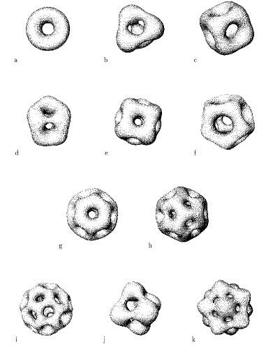
Figure C.1. Surfaces of constant baryon density for the following Skyrme fields [23]: a) $B=2$ torus b) $B=3$ tetrahedron c) $B=4$ cube d) $B=5$ with $D_{2d}$ symmetry e) $B=6$ with $D_{4d}$ symmetry f) $B=7$ dodecahedron g) $B=8$ with $D_{6d}$ symmetry h) $B=9$ with tetrahedral symmetry i) $B=17$ buckyball j) $B=5$ octahedron k) $B=11$ icosahedron.

Colophon

The manuscript was prepared in LaTeX 2ε, a standard markup format, written by Leslie Lamport in TeX typesetting language, created by Donald E. Knuth. The text is typeset in Computer Modern Roman font, combined with Computer Modern Bold Extended Roman and Computer Modern Italic. Mathematical formulas were typeset using symbols and macros provided by amsmath package for AmS-LaTeX, distributed by American Mathematical Society (AMS). Additional mathematical font shapes for Calligraphic, Doublestroke and Gotish fonts are provided by the packages calrsfs (AMS), dsfont (Olaf Kummer) and goth (Yannis Haralambour) respectively. Computer Modern font family was designed for use with TeX by D.E. Knuth.

Feynman diagrams (Fig. I.6 and Fig. I.7) were drawn using FEYNMAN package by M.J.S. Levine. Other graphics in this manuscript were drawn in PostScript graphic programming language of Adobe Systems Inc. and included in the TeX output using standard LaTeX 2ε ‘Graphics Bundle’ package designed by David Carlisle Sebastian Rahtz. The output was converted to PostScript for printing using DviPS driver program by Tomas Rokicki.