Correlator of topological charge densities at low $Q^{2}$ in QCD: connection with proton spin problem.

Abstract

Vacuum correlator of topological charge densities $\chi(q^{2})$ at low $q^{2}$ in QCD is discussed: its value $\chi(0)$ and first derivative $\chi^{\prime}(0)$ at $q^{2}=0$ and the contributions of pseudoscalar quasi-Goldstone bosons to $\chi(q^{2})$ at low $q^{2}$. The QCD sum rule [1], giving the connection of $\chi^{\prime}(0)$ (for massless quarks) with the part of the proton spin $\Sigma$, carried by $u,d,s$ quarks, is presented. From the requirement of selfconsistancy of the sum rule the values of $\chi^{\prime}(0)$ and $\Sigma$ were found. The same value of $\chi^{\prime}(0)$ follows also from the experimental data on $\Sigma$. The contributions of $\pi$ and $\eta$ to $\chi(q^{2})$ are calculated basing on low energy theorems. In such calculation the $\pi-\eta$ mixing, expressed in terms of quark mass ratios is of importance.

1. Introduction.

The existence of topological quantum number is a very specific feature of non-abelian quantum field theories and, particularly, QCD. Therefore, the study of properties of the topological charge density operator in QCD

$$Q_{5}(x)=\frac{\alpha_{s}}{8\pi}G^{n}_{\mu\nu}(x)\tilde{G}^{n}_{\mu\nu}(x)$$ (1)

and of the corresponding vacuum correlator

$$\chi(q^{2})=i\int d^{4}xe^{iqx}\langle 0\mid T\left\{Q_{5}(x),~{}Q_{5}(0)\right\}\mid 0\rangle$$ (2)

is of a great theoretical interest. (Here $G^{n}_{\mu\nu}$ is gluonic field strength tensor, $\tilde{G}_{\mu\nu}=$ $(1/2)\varepsilon_{\mu\nu\lambda\sigma}G_{\lambda\sigma}$ is its dual, $n$ are the colour indeces, $n=1,2,...N^{2}_{c}-1$, $N_{c}$ is the number of colours, $N_{c}=3$ in QCD). The existence of topological quantum numbers in non-abelian field theories was first discovered by Belavin et al.[2], their connection with non-conservation of $U(1)$ chirality was established by t’Hooft [3]. Gribov [4] was the first, who understood, that instanton configurations in Minkowski space realize the tunneling transitions between states with different topological numbers. Crewther [5] derived Ward identities related to $\chi(0)$, which allowed him to prove the theorem, that $\chi(0)=0$ in any theory where it is at least one massless quark. An important step in the investigation of the properties of $\chi(q^{2})$ was achieved by Veneziano [6] and Di Vecchia and Veneziano [7]. These authors considered the limit $~{}N_{c}\to\infty$. Assuming that in the theory there are $N_{f}$ light quarks with the masses $m_{i}\ll M$, where $M$ is the characteristic scale of strong interaction, Di Vecchia and Veneziano found that

$$\chi(0)=\langle 0\mid\bar{q}q\mid 0\rangle\Biggl{(}\sum^{N_{f}}_{i}~{}\frac{1}{m_{i}}\Biggr{)}^{-1},$$ (3)

where $\langle 0\mid\bar{q}q\mid 0\rangle$ is the common value of quark condensate for all light quarks and the terms of the order $m_{i}/M$ are neglected. The concept of $\theta$-term in the Lagrangian was succesfully exploited in [6] in deriving of (3). Using the same concept and studying the properties of the Dirac operator Leutwyler and Smilga [8] succeeded in proving eq.3 at any $N_{c}$ for the case of two light quarks, $u$ and $d$. How this method can be generalized to the case of $N_{f}=3$ is explained in the recent paper [9].

In this paper I discuss $\chi(q^{2})$ in the domain of low $\mid q^{2}\mid$, i.e. I suppose that $q^{2}/M^{2}$ is a small parameter and restrict myself to the terms linear in this ratio. In this domain must be accounted terms $\chi(0)$, $\chi^{\prime}(0)q^{2}$ as well as the contributions of low mass pseudoscalar quasi–Goldstone bosons $\pi$ and $\eta$, resulting to nonlinear $q^{2}$ dependence.

Strictly speaking, only nonperturbative part of $\chi(q^{2})$ has definite meaning. The perturbative part is divergent and its contribution depends on the renormalization procedure. For this reason only nonperturbative part of $\chi(q^{2})$ (2) with perturbative part subtracted will be considered here. In ref.1 on the basis of QCD sum rules in the external fields the connection of $\chi^{\prime}(0)$ (its nonperturbative part) with the part of the proton spin $\Sigma$, carried by $u,d,s$ quarks, was established. From the requirement of the selfconsistancy of the sum rule it was obtained

$$\chi^{\prime}(0)=(2.4\pm 0.6)\times 10^{-3}~{}GeV^{2}$$ (4)

in the limit of massless $u,d$ and $s$ quarks. The close to (4) value follows also by the use of experimental data on $\Sigma$. At low $q^{2}$ the terms, proportional to quark masses, are related to the contributions of light pseudoscalar mesons as intermediate states in the the correlator (2). These contributions are calculated below. In such calculation for the case of three quarks the mixing of $\pi^{0}$ and $\eta$ is of importance and it is accounted.

The presentation of the material in the paper is the following. In Sec.2 the QCD sum rule for $\Sigma$ is derived. The important contribution to the sum rule comes from $\chi^{\prime}(0)$. This allows to determine $\chi^{\prime}(0)$ in two ways: using the experimental data on $\Sigma$ and from the requirement of the selfconsistancy of the sum rule. Both methods give the same value of $\chi^{\prime}(0)$, given by eq.4. In Sec.3 the low energy theorems related to $\chi(0)$ are rederived with the account of possible anomalous equal-time commutator terms. (In [5]-[7] it was implicitly assumed that these terms are zero). In Sec.4 the case of one and two light quarks are considered. It is proved, that the mentioned above commutator terms are zero indeed and for the case of two quarks eq.3 is reproduced without using $N_{c}\to\infty$ limit and the concepts of $\theta$–terms. In Sec.5 the case of three $u,d,s$ light quarks is considered in the approximation $m_{u},m_{d}\ll m_{s}$. The problem of mixing of $\pi^{0}$ and $\eta$ states [10, 11] is formulated and corresponding formulae are presented. The account of $\pi-\eta$ mixing allows one to get eq.(3) from low energy theorems, formulated in Sec.2 for the case of three light quarks. (At $m_{u},m_{d}\ll m_{s}$ it coincides with the two quark case). In Sec.5 the $q^{2}$–dependence of $\chi(q^{2})$ was found at low $\mid q^{2}\mid$ in the leading nonvanishing order in $q^{2}/M^{2}$ as well as in $m_{q}/M$.

2. QCD sum rule for $\Sigma$. Connection of $\Sigma$ and $\chi^{\prime}(0)$.

As well known, the parts of the nucleon spin carried by $u,d$ and $s$-quarks are determined from the measurements of the first moment of spin dependent nucleon structure function $g_{1}(x,Q^{2})$

$$\Gamma_{p,n}(Q^{2})=\int\limits_{0}^{1}dxg_{1;p,n}(x,Q^{2})$$ (5)

The data allows one to find the value of $\Sigma$ – the part of nucleon spin carried by three flavours of light quarks $\Sigma=\Delta u+\Delta d+\Delta s$, where $\Delta u,\Delta d,\Delta s$ are the parts of nucleon spin carried by $u,d,s$ quarks. On the basis of the operator product expansion (OPE) $\Sigma$ is related to the proton matrix element of the flavour singlet axial current $j^{0}_{\mu 5}$

$$2ms_{\mu}\Sigma=\langle p,s|j^{0}_{\mu 5}|p,s\rangle,$$ (6)

where $s_{\mu}$ is the proton spin 4-vector, $m$ is the proton mass. The renormalization scheme in the calculation of perturbative QCD corrections to $\Gamma_{p,n}$ can be arranged in such a way that $\Sigma$ is scale independent.

An attempt to calculate $\Sigma$ using QCD sum rules in external fields was done in ref.[12]. Let us shortly recall the idea. The polarization operator

$$\Pi(p)=i\int d^{4}xe^{ipx}\langle 0|T\{\eta(x),\bar{\eta}(0)\}|0\rangle$$ (7)

was considered, where

$$\eta(x)=\varepsilon^{abc}\Biggl{(}u^{a}(x)C\gamma_{\mu}u^{b}(x)\Biggr{)}\gamma_{\mu}\gamma_{5}d^{c}(x)$$ (8)

is the current with proton quantum numbers [13], $u^{a},d^{b}$ are quark fields, $a,b,c$ are colour indeces. It is assumed that the term

$$\Delta L=j^{0}_{\mu 5}A_{\mu}$$ (9)

where $A_{\mu}$ is a constant singlet axial field, is added to QCD Lagrangian. In the weak axial field approximation $\Pi(p)$ has the form

$$\Pi(p)=\Pi^{(0)}(p)+\Pi^{(1)}_{\mu}(p)A_{\mu}.$$ (10)

$\Pi^{(1)}_{\mu}(p)$ is calculated in QCD by OPE at $p^{2}<0,|p^{2}|\gg R^{-2}_{c}$, where $R_{c}$ is the confinement radius. On the other hand, using dispersion relation, $\Pi^{(1)}_{\mu}(p)$ is represented by the contribution of the physical states, the lowest of which is the proton state. The contribution of excited states is approximated as a continuum and suppressed by the Borel transformation. The desired answer is obtained by equalling of these two representations. This procedure can be applied to any Lorenz structure of $\Pi^{(1)}_{\mu}(p)$ , but as was argued in [14],[15] the best accuracy can be obtained by considering the chirality conserving structure $2p_{\mu}\hat{p}\gamma_{5}$.

An essential ingredient of the method is the appearance of induced by the external field vacuum expectation values (v.e.v). The most important of them in the problem at hand is

$$\langle 0|j^{0}_{\mu 5}|0\rangle_{A}\equiv 3f^{2}_{0}A_{\mu}$$ (11)

of dimension 3. The constant $f^{2}_{0}$ is related to QCD topological susceptibility. Using (9), we can write

$$\langle 0|j^{0}_{\mu 5}|0\rangle_{A}=lim_{q\to 0}~{}i\int~{}d^{4}xe^{iqx}\langle 0|T\{j^{0}_{\nu 5}(x),j^{0}_{\mu 5}(0)\}|0\rangle A_{\nu}\equiv$$

$$\equiv lim_{q\to 0}P_{\mu\nu}(q)A_{\nu}$$ (12)

The general structure of $P_{\mu\nu}(q)$ is

$$P_{\mu\nu}(q)=-P_{L}(q^{2})\delta_{\mu\nu}+P_{T}(q^{2})(-\delta_{\mu\nu}q^{2}+q_{\mu}q_{\nu})$$ (13)

Because of anomaly there are no massless states in the spectrum of the singlet polarization operator $P_{\mu\nu}$ even for massless quarks. $P_{T,L}(q^{2})$ also have no kinematical singularities at $q^{2}=0$ . Therefore, the nonvanishing value $P_{\mu\nu}(0)$ comes entirely from $P_{L}(q^{2})$. Multiplying $P_{\mu\nu}(q)$ by $q_{\mu}q_{\nu}$, in the limit of massless $u,d,s$ quarks we get

$$q_{\mu}q_{\nu}P_{\mu\nu}(q)=-P_{L}(q^{2})q^{2}=N^{2}_{f}(\alpha_{s}/4\pi)^{2}i\int~{}d^{4}xe^{iqx}\times$$

$$\times\langle 0|T{G^{n}_{\mu\nu}(x)\tilde{G}^{n}_{\mu\nu}(x),G^{m}_{\lambda\sigma}(0)\tilde{G}^{m}_{\lambda\sigma}(0)}|0\rangle,$$ (14)

where $G^{n}_{\mu\nu}$ is the gluonic field strength, $\tilde{G}_{\mu\nu}=(1/2)\varepsilon_{\mu\nu\lambda\sigma}G_{\lambda\sigma}$.(The anomaly condition was used, $N_{f}=3$.). Going to the limit $q^{2}\to 0$, we have

$$f^{2}_{0}=-(1/3)P_{L}(0)=\frac{4}{3}N^{2}_{f}\chi^{\prime}(0),$$ (15)

where $\chi(q^{2})$ is defined by (2).

According to Crewther theorem [5]), $\chi(0)=0$ if there is at least one massless quark. The attempt to find $\chi^{\prime}(0)$ itself by QCD sum rules failed: it was found [12] that OPE does not converge in the domain of characteristic scales for this problem. However, it was possible to derive the sum rule, expressing $\Sigma$ in terms of $f^{2}_{0}$ (11) or $\chi^{\prime}(0)$. The OPE up to dimension $d=7$ was performed in ref.[12]. Among the induced by the external field v.e.v.’s besides (11), the v.e.v. of the dimension 5 operator

$$g\langle 0|\sum\limits_{q}\bar{q}\gamma_{\alpha}(1/2)\lambda^{n}\tilde{G}^{n}_{\alpha\beta}q|0\rangle_{A}\equiv 3h_{0}A_{\beta},~{}~{}~{}q=u,d,s$$ (16)

was accounted and the constant $h_{0}$ was estimated using a special sum rule,
$h_{0}\approx 3\times 10^{-4}GeV^{4}$ . There were also accounted the gluonic condensate $d=4$ and the square of quark condensate $d=6$ (both times the external $A_{\mu}$ field operator, $d=1$). However, the accuracy of the calculation was not good enough for reliable calculation of $\Sigma$ in terms of $f^{2}_{0}$: the necessary requirement of the method – the weak dependence of the result on the Borel parameter was not well satisfied.

In [1] the accuracy of the calculation was improved by going to higher order terms in OPE up to dimension 9 operators. Under the assumption of factorization – the saturation of the product of four-quark operators by the contribution of an intermediate vacuum state – the dimension 8 v.e.v.’s are accounted (times $A_{\mu}$):

$$-g\langle 0|\bar{q}\sigma_{\alpha\beta}(1/2)\lambda^{n}G^{n}_{\alpha\beta}q\cdot\bar{q}q|0\rangle=m^{2}_{0}\langle 0|\bar{q}q|0\rangle^{2},$$ (17)

where $m^{2}_{0}=0.8\pm 0.2~{}GeV^{2}$ was determined in [16]. In the framework of the same factorization hypothesis the induced by the external field v.e.v. of dimension 9

$$\alpha_{s}\langle 0|j^{(0)}_{\mu 5}|0\rangle_{A}\langle 0|\bar{q}q|0\rangle^{2}$$ (18)

is also accounted. In the calculation the following expression for the quark Green function in the constant external axial field was used [15]:

$$\langle 0|T\{q^{a}_{\alpha}(x),~{}\bar{q}^{b}_{\beta}(0)\}|0\rangle_{A}=i\delta^{ab}\hat{x}_{\alpha\beta}/2\pi^{2}x^{4}+$$

$$+(1/2\pi^{2})\delta^{ab}(Ax)(\gamma_{5}\hat{x})_{\alpha\beta}/x^{4}-(1/12)\delta^{ab}\delta_{\alpha\beta}\langle 0|\bar{q}q|0\rangle+$$

$$+(1/72)i\delta^{ab}\langle 0|\bar{q}q|0\rangle(\hat{x}\hat{A}\gamma_{5}-\hat{A}\hat{x}\gamma_{5})_{\alpha\beta}+$$

$$+(1/12)f^{2}_{0}\delta^{ab}(\hat{A}\gamma_{5})_{\alpha\beta}+(1/216)\delta^{ab}h_{0}\Biggl{[}(5/2)x^{2}\hat{A}\gamma_{5}-(Ax)\hat{x}\gamma_{5}\Biggr{]}_{\alpha\beta}$$ (19)

The terms of the third power in $x$-expansion of quark propagator proportional to $A_{\mu}$ are omitted in (19), because they do not contribute to the tensor structure of $\Pi_{\mu}$ of interest. Quarks are considered to be in the constant external gluonic field and quark and gluon QCD equations of motion are exploited (the related formulae are given in [17]). There is also an another source of v.e.v. $h_{0}$ to appear besides the $x$-expansion of quark propagator given in eq.(19): the quarks in the condensate absorb the soft gluonic field emitted by other quark. A similar situation takes place also in the calculation of the v.e.v. (18) contribution. The accounted diagrams with dimension 9 operators have no loop integrations. There are others v.e.v. of dimensions $d\leq 9$ particularly containing gluonic fields. All of them, however, correspond to at least one loop integration and are suppressed by the numerical factor $(2\pi)^{-2}$. For this reason they are disregarded.

The sum rule for $\Sigma$ is given by

$$\Sigma+C_{0}M^{2}=-1+\frac{8}{9\tilde{\lambda}^{2}_{N}}e^{m^{2}/M^{2}}\left\{a^{2}L^{4/9}+6\pi^{2}f^{2}_{0}M^{4}E_{1}\Biggl{(}\frac{W^{2}}{M^{2}}\Biggr{)}L^{-4/9}+\right.$$

$$\left.+14\pi^{2}h_{0}M^{2}E_{0}\Biggl{(}\frac{W^{2}}{M^{2}}\Biggr{)}L^{-8/9}-\frac{1}{4}~{}\frac{a^{2}m^{2}_{0}}{M^{2}}-\frac{1}{9}\pi\alpha_{s}f^{2}_{0}~{}\frac{a^{2}}{M^{2}}\right\}$$ (20)

Here $M^{2}$ is the Borel parameter, $\tilde{\lambda}_{N}$ is defined as $\tilde{\lambda}^{2}_{N}=32\pi^{4}\lambda^{2}_{N}=2.1~{}GeV^{6}$, $\langle 0|\eta|p\rangle=\lambda_{N}v_{p},$ where $v_{p}$ is proton spinor, $W^{2}$ is the continuum threshold, $W^{2}=2.5~{}GeV^{2}$,

$$a=-(2\pi)^{2}\langle 0|\bar{q}q|0\rangle=0.55~{}GeV^{3}$$ (21)

$$E_{0}(x)=1-e^{-x},~{}~{}~{}E_{1}(x)=1-(1+x)e^{-x}$$

$L=ln(M/\Lambda)/ln(\mu/\Lambda),~{}~{}~{}\Lambda=\Lambda_{QCD}=200~{}MeV$ and the normalization point $\mu$ was chosen $\mu=1~{}GeV$. When deriving (20) the sum rule for the nucleon mass was exploited what results in appearance of the first term, -1, in the right hand side (rhs) of (20). This term absorbs the contributions of the bare loop, gluonic condensate as well as $\alpha_{s}$ corrections to them and essential part of terms, proportional to $a^{2}$ and $m^{2}_{0}a^{2}$. The values of the parameters, $a,\tilde{\lambda}^{2}_{N},W^{2}$ taken above were chosen by the best fit of the sum rules for the nucleon mass (see [18], Appendix B) performed at $\Lambda=200~{}MeV$. It can be shown, using the value of the ratio $2m_{s}/(m_{u}+m_{d})=24.4\pm 1.5$ [19] that $a(1~{}GeV)=0.55~{}GeV^{3}$ corresponds to $m_{s}(1~{}GeV)=153~{}MeV$. $\alpha_{s}$ corrections are accounted in the leading order (LO) what results in appearance of anomalous dimensions. Therefore $\Lambda$ has the meaning of effective $\Lambda$ in LO. The unknown constant $C_{0}$ in the left-hand side (lhs) of (20) corresponds to the contribution of inelastic transitions $p\to N^{*}\to interaction~{}withA_{\mu}\to p$ (and in inverse order). It cannot be determined theoretically and may be found from $M^{2}$ dependence of the rhs of (20) (for details see [18, 20]). The necessary condition of the validity of the sum rule is $|\Sigma|\gg|C_{0}M^{2}|exp[(-W^{2}+m^{2})/M^{2}]$ at characteristic values of $M^{2}$ [20]. The contribution of the last term in the rhs of (20)) is negligible. The sum rule (20) as well as the sum rule for the nucleon mass is reliable in the interval of the Borel parameter $M^{2}$ where the last term of OPE is small, less than $10-15\%$ of the total and the contribution of continuum does not exceed $40-50\%$. This fixes the interval $0.85<M^{2}<1.4~{}GeV^{2}$.The $M^{2}$-dependence of the rhs of (20) at $f^{2}_{0}=3\times 10^{-2}~{}GeV^{2}$ is plotted in fig.1a. The complicated expression in rhs of (20) is indeed an almost linear function of $M^{2}$ in the given interval! This fact strongly supports the reliability of the approach. The best values of $\Sigma=\Sigma^{fit}$ and $C_{0}=C^{fit}_{0}$ are found from the $\chi^{2}$ fitting procedure

$$\chi^{2}=\frac{1}{n}\sum\limits^{n}_{i=1}~{}[\Sigma^{fit}-C^{fit}_{0}M^{2}_{i}-R(M^{2}_{i})]^{2}=min,$$ (22)

where $R(^{2})$ is the rhs of (20).

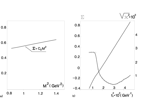
Fig. 1.: a) The $M^{2}$-dependence of $\Sigma+C_{0}M^{2}$ at $f^{2}_{0}=3\times 10^{-2}~{}GeV^{2}$; b) $\Sigma$ (solid line, left ordinate axis) and $\sqrt{\chi^{2}}$, (dashed line, right ordinate axis). as a functions of $f^{2}_{0}$.

The values of $\Sigma$ as a function of $f^{2}_{0}$ are plotted in fig.1b together with $\sqrt{\chi^{2}}$. In our approach the gluonic contribution cannot be separated and is included in $\Sigma$. The experimental value of $\Sigma$ can be estimated [21, 22] (for discussion see [23]) as $\Sigma=0.3\pm 0.1$. Then from fig.1b we have $f^{2}_{0}=(2.8\pm 0.7)\times 10^{-2}~{}GeV^{2}$ and $\chi^{\prime}(0)=(2.3\pm 0.6)\times 10^{-3}~{}GeV^{2}$. The error in $f^{2}_{0}$ and $\chi^{\prime}$ besides the experimentall error includes the uncertainty in the sum rule estimated as equal to the contribution of the last term in OPE (two last terms in Eq.(20) and a possible role of NLO $\alpha_{s}$ corrections. Allowing the deviation of $\sqrt{\chi^{2}}$ by a factor 1.5 from the minimum we get $\chi^{\prime}=(24\pm 0.6)\times 10^{-3}GeV^{2}$ and $\Sigma=0.32\pm 0.17$ from the requirement of selfconsistency of the sum rule. At $f^{2}_{0}=2.8\times 10^{-2}~{}GeV^{2}$ the value of the constant $C_{0}$ found from the fit is $C_{0}=0.19~{}GeV^{-2}$. Therefore, the mentioned above necessary condition of the sum rule validity is well satisfied.

Let us discuss the role of various terms of OPE in the sum rules (20). To analyze it the sum rule (20) was considered for 4 different cases, i.e. when it is taken into consideration: a) only contribution of the operators up to d=3 (the term –1 and the term, proportional to $f^{2}_{0}$ in (20)); b) contribution of the operators up to d=5 (the term $\sim h_{0}$ is added); c) contribution of the operators up to d=7 (three first terms in (20)), d) the result (20), i.e. all operators up to d=9. For this analysis the value of $f^{2}_{0}=0.03~{}GeV^{2}$ was chosen, but the conclusion appears to be the same for all more or less reasonable choice of $f^{2}_{0}$. Results of the fit of the sum rules are shown in Table 1 for all four cases. The fit is done in the region of Borel masses $0.9<M^{2}<1.3~{}GeV^{2}$. In the first column the values of $\Sigma$ are shown , in the second - values of the parameter C, and in the third - the ratio $\gamma=|\sqrt{\chi^{2}}/\Sigma|$, which is the real parameter, describing reliability of the fit. From the table one can see, that reliability of the fit monotonously improves with increasing of the number of accounted terms of OPE and is quite satisfactory in the case $d$

Table 1.:

case	$\Sigma$	$C(GeV^{-2})$	$\gamma$
a)	-0.019	0.31	$10^{-1}$
b)	0.031	0.3	$5.10^{-2}$
c)	0.54	0.094	$9.10^{-3}$
d)	0.36	0.21	$1.3\cdot 10^{-3}$

3. Low energy theorems.

Consider QCD with $N_{f}$ light quarks, $m_{i}\ll M\sim 1~{}GeV$, $i=1,...N_{f}$. Define the singlet (in flavour) axial current by

$$j_{\mu 5}(x)=\sum^{N_{f}}_{i}\bar{q}_{i}(x)\gamma_{\mu}\gamma_{5}q(x)$$ (23)

and the polarization operator

$$P_{\mu\nu}(q)=i\int d^{4}xe^{iqx}\langle 0\mid T~{}\{j_{\mu 5}(x),j_{\mu 5}(0)~{}\}\mid 0\rangle.$$ (24)

The general form of the polarization operator is:

$$P_{\mu\nu}(q)=-P_{L}(q^{2})\delta_{\mu\nu}+P_{T}(q^{2})(-\delta_{\mu\nu}q^{2}+q_{\mu}q_{\nu})$$ (25)

Because of anomaly the singlet axial current is nonconserving:

$$\partial_{\mu}j_{\mu 5}(x)=2N_{f}Q_{5}(x)+D(x),$$ (26)

where $Q_{5}(x)$ is given by (1) and

$$D(x)=2i\sum^{N_{f}}_{i}m_{i}\bar{q}_{i}(x)\gamma_{5}q_{i}(x)$$ (27)

It is well known, that even if some light quarks are massless, the corresponding Goldstone bosons, arising from spontaneous violation of chiral symmetry do not contribute to singlet axial channel (it is the solution of $U(1)$ problem), i.e. to polarization operator $P_{\mu\nu}(q)$. $P_{L}(q^{2})$ also have no kinematical singularities at $q^{2}=0$. Therefore

$$P_{\mu\nu}(q)q_{\mu}q_{\nu}=-P_{L}(q^{2})q^{2}$$ (28)

vanishes in the limit $q^{2}\to 0$. Calculate the left-hand side (lhs) of (28) in the standard way – put $q_{\mu}q_{\nu}$ inside the integral in (24) and integrate by parts. (For this it is convenient to represent the polarization operator in the coordinate space as a function of two coordinates $x$ and $y$.) Going to the limit $q^{2}\to 0$ we have

$$\lim_{q^{2}\to 0}P_{\mu\nu}(q)q_{\mu}q_{\nu}=i\int d^{4}x\langle 0\mid T\{2N_{f}Q_{5}(x),~{}2N_{f}Q_{5}(0)$$

$$+2N_{f}Q_{5}(x),~{}D(0)+D(x),~{}2N_{f}Q_{5}(0)+D(x),~{}D(0)\}\mid 0\rangle$$

$$+4\sum^{N_{f}}_{i}m_{i}\langle\mid\bar{q}_{i}(0)q_{i}(0)\mid 0\rangle$$

$$+\int d^{4}x\langle 0\mid~{}[j_{05}(x),~{}2N_{f}Q_{5}(0)~{}]\mid 0\rangle\delta(x_{0})=0$$ (29)

In the calculation of (29) the anomaly condition (26) was used. The terms, proportional to quark condensates arise from equal time commutator $[j_{05}(x)$, $D(0)]_{x_{0}=0}$, calculated by standard commutation relations. Relation (29) up to the last term was first obtained by Crewther [5]. The last term, equal to zero according to standard commutation relations and omitted in [5]-[7], is keeped. The reason is, that we deal with very subtle situation, related to anomaly, where nonstandard Schwinger terms in commutation relations may appear. (It can be shown, that, in general the only Schwinger term in this problem is given by the last term in the lhs of (29): no others can arise.) Consider also the correlator:

$$P_{\mu}(q)=i\int d^{4}x~{}e^{iqx}\langle 0\mid T\{j_{\mu 5}(x),~{}Q_{5}(0)\}\mid 0\rangle$$ (30)

and the product $P_{\mu}(q)q_{\mu}$ in the limit $q^{2}\to 0$ (or $q^{2}$ of order of the $m^{2}_{\pi}$, where $m_{\pi}$ is the mass of Goldstone boson). The general form of $P_{\mu}(q)$ is $P_{\mu}(q)=Aq_{\mu}$. Therefore nonvanishing values of $P_{\mu}q_{\mu}$ in the limit $q^{2}\to 0$ (or of order of quark mass $m$, if $\mid q^{2}\mid\sim m^{2}_{\pi}$ – this limit will be also intersting for us later) can arise only from Goldstone bosons intermediate states in (30). Let us us estimate the corresponding matrix elements

$$\langle 0\mid j_{\mu 5}\mid\pi\rangle=Fq_{\mu}$$ (31)

$$\langle 0\mid Q_{5}\mid\pi\rangle=F^{\prime}$$ (32)

$F$ is of order of $m$, since in the limit of massless quarks Goldstone bosons are coupled only to nonsinglet axial current. $F^{\prime}$ is of order of $m^{2}_{\pi}f_{\pi}\sim m$, where $f_{\pi}$ is the pion decay constant (not considered to be small), since in massless quark limit, the Goldstone boson is decoupled from $Q_{5}$ . These estimations give

$$P_{\mu}q_{\mu}\sim\frac{q^{2}}{q^{2}-m^{2}_{\pi}}m^{2}$$ (33)

and it is zero at $q^{2}\to 0,~{}m^{2}_{\pi}\not=0$ and of order of $m^{2}$ at $q^{2}\sim m^{2}_{\pi}$. In what follows I will restrict myself by the terms linear in quark masses. So, I can put $P_{\mu}(q)q_{\mu}=0$ at $q\to 0$. The integration by parts, in the right-hand side (rhs) of (30) gives:

$$\lim_{q^{2}\to 0}P_{\mu}(q)q_{\mu}=-\int d^{4}x\langle 0\mid T\{2N_{f}Q_{5}(x),~{}Q_{5}(0)+D(x),~{}Q_{5}(0)\}\mid 0\rangle$$

$$-\int d^{4}x\langle 0\mid[~{}j_{05}(x),~{}Q_{5}(0)~{}]\mid 0\rangle\delta(x_{0})=0$$ (34)

After the substitution of (3.) in (29) arise the low energy theorem:

$$i\int d^{4}x\langle 0\mid T\{2N_{f}Q_{5}(x),~{}2N_{f}Q_{5}(0)\}\mid 0\rangle$$

$$-i\int d^{4}x\langle 0\mid T\{D(x),~{}D(0)\}\mid 0\rangle-4\sum^{N_{f}}_{i}m_{i}\langle 0\mid\bar{q}_{i}(0)q_{i}(0)\mid 0\rangle$$

$$+i\int d^{4}x\langle 0\mid[~{}j^{0}_{05}(x),~{}2N_{f}Q_{5}(0)~{}]\mid 0\rangle\delta(x_{0})=0$$ (35)

The low energy theorem (35), with the last term in the lhs omitted, was found by Crewther [5].

4. One and two light quarks.

Consider first the case of one massless quark, $N_{f}=1$, $m=0$. This case can easily be treated by introduction of $\theta$-term in the Lagrangian,

$$\Delta L=\theta\frac{\alpha_{s}}{4\pi}~{}G^{n}_{\mu\nu}\tilde{G}^{n}_{\mu\nu}$$ (36)

The matrix element $\langle 0\mid Q_{5}\mid n\rangle$ between any hadronic state $\mid n\rangle$ and vacuum is proportional

$$\int d^{4}x\langle 0\mid Q_{5}(x)\mid n\rangle\sim\langle 0\mid\frac{\partial}{\partial\theta}lnZ\mid n\rangle_{\theta=0},$$ (37)

where $Z=e^{iL}$ and $L$ is the Lagrangian. The gauge transformation of the quark field $\psi^{\prime}\to e^{i\alpha\gamma_{5}}\psi$ results to appearance of the term

$$\delta L=\alpha\partial_{\mu}j_{\mu 5}=\alpha(\alpha_{s}/4\pi)G^{n}_{\mu\nu}\tilde{G}^{n}_{\mu\nu}$$ (38)

in the Lagrangian. By the choice $\alpha=-\theta$ the $\theta$-term (36) will be killed and $(\partial/\partial\theta)lnZ=0$. Therefore, $\chi(0)=0$ (Crewther theorem). The first term in (35) vanishes, as well as the second and third, since $m=0$. From (35) we have, that indeed the anomalous commutator vanishes

$$\langle 0\mid[~{}j_{05}(x),~{}Q_{5}(0)~{}]_{x_{0}=0}\mid 0\rangle=0,$$ (39)

supporting the assumptions done in [5]-[7].

Let us turn now to the case of two light quarks, $u,d,N_{f}=2$. This is the case of real QCD, where the strange quark is considered as a heavy. Define the isovector axial current

$$j^{(3)}_{\mu 5}=(\bar{u}\gamma_{\mu}\gamma_{5}u-\bar{d}\gamma_{\mu}\gamma_{5}d)/\sqrt{2}$$ (40)

and its matrix element between the states of pion and vacuum

$$\langle 0\mid j^{(3)}_{\mu 5}\mid\pi\rangle=f_{\pi}q_{\mu},$$ (41)

where $q_{\mu}$ is pion 4-momentum, $f_{\pi}=133~{}MeV$. Multiply (41) by $q_{\mu}$. Using Dirac equations for quark fields, we have

$$\frac{2i}{\sqrt{2}}\langle 0\mid m_{u}\bar{u}\gamma_{5}u-m_{d}\bar{d}\gamma_{5}d\mid\pi\rangle=\frac{i}{\sqrt{2}}\langle 0\mid(m_{u}+m_{d})(\bar{u}\gamma_{5}u-\bar{d}\gamma_{5}d)$$

$$+(m_{u}-m_{d})((\bar{u}\gamma_{5}u+\bar{d}\gamma_{5}d)\mid\pi\rangle=f_{\pi}m^{2}_{\pi},$$ (42)

where $m_{u}$, $m_{d}$ are $u$ and $d$ quark masses. The ratio of the matrix elements in lhs of (42) is of order

$$\frac{\langle 0\mid\bar{u}\gamma_{5}u+\bar{d}\gamma_{5}d\mid\pi\rangle}{\langle 0\mid\bar{u}\gamma_{5}u-\bar{d}\gamma_{5}d\mid\pi\rangle}\sim\frac{m_{u}-m_{d}}{M},$$ (43)

since the matrix element in the numerator violates isospin and this violaton (in the absence of elecntomagnetism, which is assumed) can arise from the difference $m_{u}-m_{d}$ only. Neglecting this matrix element we have from (42)

$$\frac{i}{\sqrt{2}}\langle 0\mid\bar{u}\gamma_{5}u-\bar{d}\gamma_{5}d\mid\pi\rangle=\frac{f_{\pi}m^{2}_{\pi}}{m_{u}+m_{d}}$$ (44)

Let us find $\chi(0)$ from low energy sum rule (35) restricting ourself to the terms linear in quark masses. Since $D(x)\sim m$, the only intermediate state contributing to the matrix element

$$\int d^{4}x\langle 0\mid T\{D(x),~{}D(0)\}\mid 0\rangle$$ (45)

in (35) is the one-pion state. Define

$$D_{q}=2i(m_{u}\bar{u}\gamma_{5}u+m_{d}\bar{d}\gamma_{5}d).$$ (46)

Then

$$\langle 0\mid D_{q}\mid\pi\rangle=i\langle 0\mid(m_{u}+m_{d})(\bar{u}\gamma_{5}u+\bar{d}\gamma_{5}d)+(m_{u}-m_{d})(\bar{u}\gamma_{5}u-\bar{d}\gamma_{5}d)\mid\pi\rangle$$

$$=\sqrt{2}\frac{m_{u}-m_{d}}{m_{u}+m_{d}}f_{\pi}m^{2}_{\pi},$$ (47)

where the matrix element of singlet axial current was neglected and (44) was used. The substitution of (47) into (45) gives

$$i\int d^{4}xe^{iqx}\langle 0\mid T\{D_{q}(x),~{}D_{q}(0)\}\mid 0\rangle_{q\to 0}=\lim_{q\to 0}\left\{-\frac{1}{q^{2}-m^{2}_{\pi}}2\Biggl{(}\frac{m_{u}-m_{d}}{m_{u}+m_{d}}\Biggr{)}^{2}f^{2}_{\pi}m^{2}_{\pi}\right\}$$

$$=-4\frac{(m_{u}-m_{d})^{2}}{m_{u}+m_{d}}\langle 0\mid\bar{q}q\mid 0\rangle$$ (48)

In the last equality in (48) Gell-Mann-Oakes-Renner relation [24]

$$\langle 0\mid\bar{q}q\mid 0\rangle=-\frac{1}{2}~{}\frac{f^{2}_{\pi}m^{2}_{\pi}}{m_{u}+m_{d}}$$ (49)

was substituted as well the $SU(2)$ equalities

$$\langle 0\mid\bar{u}u\mid 0\rangle=\langle 0\mid\bar{d}d\mid 0\rangle\equiv\langle 0\mid\bar{q}q\mid 0\rangle.$$ (50)

From (35) and (48) we finally get:

$$\chi(0)=i\int d^{4}x\langle 0\mid T\{Q_{5}(x),~{}Q_{5}(0)\}\mid 0\rangle=\frac{m_{u}m_{d}}{m_{u}+m_{d}}\langle 0\mid\bar{q}q\mid 0\rangle$$ (51)

in concidence with eq.3.

In a similar way matrix element $\langle 0\mid Q_{5}\mid\pi\rangle$ can be found. Consider

$$\langle 0\mid j_{\mu 5}\mid\pi\rangle=Fq_{\mu}$$ (52)

The estimation of $F$ gives

$$F\sim\frac{m_{u}-m_{d}}{M}f_{\pi}$$ (53)

and after multiplying of (52) by $q_{\mu}$ the rhs of (52) can be neglected. In the lhs we have

$$\langle 0\mid D_{q}\mid\pi\rangle+2N_{f}\langle 0\mid Q_{5}\mid\pi\rangle=0$$ (54)

The substitution of (47) into (54) results in

$$\langle 0\mid Q_{5}\mid\pi\rangle=-\frac{1}{2\sqrt{2}}\frac{m_{u}-m_{d}}{m_{u}+m_{d}}f_{\pi}m^{2}_{\pi}$$ (55)

The relation of this type (with a wrong numerical coefficient) was found in [11], the correct formula was presented in [25]. From comparison of (51) and (55) it is clear, that it would be wrong to calculate $\chi(0)$ by accounting only pions as intermediate states in the lhs of (51) – the constant terms, reflecting the necessity of subtraction terms in dispersion relation and represented by proportional to quark condensate terms in (35) are extremingly important. The cancellation of Goldstone bosons pole terms and these constant terms results in the Crewther theorem – the vanishing of $\chi(0)$, when one of the quark masses, e.g. $m_{u}$ is going to zero.

5. Three light quarks.

Let us dwell on the real QCD case of three light quarks, $u,d$ and $s$. Since the ratios $m_{u}/m_{s}$, $m_{d}/m_{s}$ are small, less than 1/20, account them only in the leading order. When the $u$ and $d$ quark masses $m_{u}$ and $m_{d}$ are not assumed to be equal, the quasi-Goldstone states $\pi^{0}$ and $\eta$ are no more states of pure isospin 1 and 0 correspondingly: in both of these states persist admixture of other isospin [10, 11] proporional to $m_{u}-m_{d}$. (The violation of isospin by electromagnetic interaction is small in the problem under investigation [10] and can be neglected. The $\eta^{\prime}-\eta$ mixing is also neglected.) In order to treat the problem it is convenient to introduce pure isospin 1 and 0 pseudoscalar meson fields $\varphi_{3}$ and $\varphi_{8}$ in $SU(3)$ octet and the corresponding states $\mid P_{3}\rangle$, $\mid P_{8}\rangle$ [10, 25]. Then in the $SU(3)$ limit

$$\langle 0\mid j^{(3)}_{\mu 5}\mid P_{3}\rangle=f_{\pi}q_{\mu}$$ (56)

$$\langle 0\mid j^{(8)}_{\mu 5}\mid P_{8}\rangle=f_{\pi}q_{\mu},$$ (57)

where

$$j^{(8)}_{\mu 5}=(\bar{u}\gamma_{\mu}\gamma_{5}u+\bar{d}\gamma_{\mu}\gamma_{5}d-2\bar{s}\gamma_{\mu}\gamma_{5}s)/\sqrt{6}$$ (58)

and $j^{(3)}_{\mu 5}$ is given by (40). The states $\mid P_{3}\rangle$, $\mid P_{8}\rangle$ are not eigenstates of the Hamiltonian. In the free Hamiltonian

$$H=\frac{1}{2}\tilde{m}^{2}_{\pi}\varphi^{2}_{3}+\frac{1}{2}\tilde{m}^{2}_{\eta}\varphi^{2}_{8}+\langle P_{8}\mid P_{3}\rangle\varphi_{3}\varphi_{8}+\mbox{kinetic terms}$$ (59)

the nondiagonal term $\sim\varphi_{3}\varphi_{8}$ is present ( $\tilde{m}^{2}_{\pi}$ and $\tilde{m}^{2}_{\eta}$ in (59) coincides with $m^{2}_{\pi}$ and $m^{2}_{\eta}$ up to terms quadratic in $\langle P_{8}\mid P_{3}\rangle$). The nondiagonal term was calculated in [10] on the basis of PCAC and current algebra (see also [11])

$$\langle P_{8}\mid P_{3}\rangle=\frac{1}{\sqrt{3}}m^{2}_{\pi}\frac{m_{u}-m_{d}}{m_{u}+m_{d}}$$ (60)

The physical $\pi$ and $\eta$ states arise after orthogonalization of the Hamiltonian (59)

$$\mid\pi\rangle=cos\theta\mid P_{3}\rangle-sin\theta\mid P_{8}\rangle$$

$$\mid\eta\rangle=sin\theta\mid P_{3}\rangle+cos\theta\mid P_{8}\rangle$$ (61)

where the mixing angle $\theta$ is given by (at small $\theta$) [10, 11]:

$$\theta=\frac{\langle P_{8}\mid P_{3}\rangle}{m^{2}_{\eta}-m^{2}_{\pi}}\approx\frac{\langle P_{8}\mid P_{3}\rangle}{m^{2}_{\eta}}=\frac{1}{\sqrt{3}}~{}\frac{m^{2}_{\pi}}{m^{2}_{\eta}}~{}\frac{m_{u}-m_{d}}{m_{u}+m_{d}}$$ (62)

In terms of the fields $\varphi_{3}$ and $\varphi_{8}$ PCAC relations take the form [10];

$$\partial_{\mu}j^{(3)}_{\mu 5}=f_{\pi}(m^{2}_{\pi}\varphi_{3}+\langle P_{8}\mid P_{3}\rangle\varphi_{8})$$ (63)

$$\partial_{\mu}j^{(8)}_{\mu 5}=f_{\pi}(m^{2}_{\pi}\varphi_{8}+\langle P_{8}\mid P_{3}\rangle\varphi_{3})$$ (64)

Our goal now is to calculate the contribution of pseudoscalar octet states to the second term in the lhs of (35). It is convenient to use the full set of orthogonal states $\mid P_{3}\rangle$, $\mid P_{8}\rangle$ as the basis. Use the notation

$$D=D_{q}+D_{s}~{}~{}~{}~{}~{}~{}~{}~{}D_{s}=2im_{s}\bar{s}\gamma_{5}s,$$ (65)

where $D_{q}$ is given by (46). The matrix element

$$\langle 0\mid D_{q}\mid P_{3}\rangle=\sqrt{2}\frac{m_{u}-m_{d}}{m_{u}+m_{d}}f_{\pi}m^{2}_{\pi}$$ (66)

can be found by the same argumentation, as that was used in the derivation of (47). In order to find $\langle 0\mid D_{q}\mid P_{8}\rangle$ take the matrix element of eq.63 between vacuum and $\mid P_{8}\rangle$

$$\langle 0\mid\partial_{\mu}j^{(3)}_{\mu 5}\mid P_{3}\rangle=f_{\pi}\langle P_{8}\mid P_{3}\rangle$$ (67)

The substitution in the lhs of (67) of the expression for $\partial_{\mu}j^{(3)}_{\mu 5}$ through quark fields gives

$$\langle 0\mid\bar{u}\gamma_{5}u-\bar{d}\gamma_{5}d\mid P_{8}\rangle=-\frac{m_{u}-m_{d}}{m_{u}+m_{d}}\langle 0\mid\bar{u}\gamma_{5}u+\bar{d}\gamma_{5}d\mid P_{8}\rangle-$$

$$-i\sqrt{\frac{2}{3}}f_{\pi}m^{2}_{\pi}\frac{m_{u}-m_{d}}{(m_{u}+m_{d})^{2}}$$ (68)

In a similar way take matrix element of eq. (64) between $\langle 0\mid$ and $\mid P_{8}\rangle$ and substitute into it (68). We get

$$\frac{i}{\sqrt{6}}\langle 0\mid\Biggl{[}m_{u}+m_{d}-\frac{(m_{u}-m_{d})^{2}}{m_{u}+m_{d}}\Biggr{]}(\bar{u}\gamma_{5}u+\bar{d}\gamma_{5}d)-4m_{s}\bar{s}\gamma_{5}s\mid P_{8}\rangle$$

$$=f^{2}_{\pi}m^{2}_{\eta}-\frac{1}{3}m^{2}_{\pi}f_{\pi}\Biggl{(}\frac{m_{u}-m_{d}}{m_{u}+m_{d}}\Biggr{)}^{2}$$ (69)

As follows from $SU(3)$ symmetry of strong interaction

$$\langle 0\mid\bar{u}\gamma_{5}u+\bar{d}\gamma_{5}d\mid P_{8}\rangle=-\langle 0\mid\bar{s}\gamma_{5}s\mid P_{8}\rangle$$ (70)

up to terms of order $m_{q}/M$, which are neglected. From (69),(70) we find:

$$\langle 0\mid D_{s}\mid P_{8}\rangle=-\sqrt{\frac{3}{2}}f_{\pi}m^{2}_{\eta}\Biggl{[}1-\frac{1}{4}\frac{(m_{u}-m_{d})^{2}}{m_{s}(m_{u}+m_{d})}\Biggr{]}\Biggl{[}1+\frac{m_{u}m_{d}}{m_{s}(m_{u}+m_{d})}\Biggr{]}$$ (71)

$$\langle 0\mid D_{q}\mid P_{8}\rangle=4\sqrt{\frac{2}{3}}f_{\pi}m^{2}_{\pi}\frac{m_{u}m_{d}}{(m_{u}+m_{d})^{2}}$$ (72)

in notation (46),(65). When deriving (71) the $SU(3)$ relation

$$m^{2}_{\eta}=\frac{4}{3}m^{2}_{\pi}\frac{m_{s}}{m_{u}+m_{d}}\Biggl{(}1-\frac{1}{4}\frac{m_{u}+m_{d}}{m_{s}}\Biggr{)}$$ (73)

was used. In (71) the small terms $\sim m_{u}/m_{s}$, $m_{d}/m_{s}$ are accounted, because they are multiplyed by large factor $m^{2}_{\eta}$. In (72) small terms are disregarded. The matrix element $\langle 0\mid D_{s}\mid P_{3}\rangle$ can be found from (64). We have

$$\frac{1}{\sqrt{6}}\langle 0\mid D_{q}-2D_{s}\mid P_{3}\rangle=f_{\pi}\langle P_{8}\mid P_{3}\rangle$$ (74)

The substitution of (66) and (60) into (74) gives

$$\langle 0\mid D_{s}\mid P_{3}\rangle=0$$ (75)

Equations (66),(71),(72) and (75) allow one to calculate the interesting for us correlator

$$i\int d^{4}x\langle 0\mid T\{D(x),~{}D(0)\}\mid 0\rangle$$ (76)

when the sets $\mid P_{3}\rangle\langle P_{3}\mid$ and $\mid P_{8}\rangle\langle P_{8}\mid$ are taken as intermediate states. But $\mid P_{3}\rangle,~{}\mid P_{8}\rangle$ are not the eigenstates of the Hamiltonian, they mix in accord with (59). Therefore the transitions $\langle P_{8}\mid P_{3}\rangle$ arising from the mixing term in (59) must be also accounted. There are two such terms. The one corresponds to the transition $\langle 0\mid D_{s}\mid P_{8}\rangle$ $\langle P_{3}\mid D_{q}\mid 0\rangle$ and its contribution to (66) is given by

$$\lim_{q^{2}\to 0}\left\{-2\langle 0\mid D_{s}\mid P_{8}\rangle\frac{1}{q^{2}-m^{2}_{\eta}}\langle P_{8}\mid P_{3}\rangle\frac{1}{q^{2}-m^{2}_{\pi}}\langle P_{3}\mid D_{q}\mid 0\rangle\right\}=$$

$$=2f^{2}_{\pi}m^{2}_{\pi}\Biggl{(}\frac{m_{u}-m_{d}}{m_{u}+m_{d}}\Biggr{)}^{2}$$ (77)

The other corresponds to the transition between two $D_{s}$ operators, where $\langle P_{3}\mid P_{3}\rangle$ enter as intermediate state. This contribution is equal to:

$$\lim_{q^{2}\to 0}\left\{-\langle 0\mid D_{s}\mid P_{8}\rangle\frac{1}{q^{2}-m^{2}_{\eta}}\langle P_{8}\mid P_{3}\rangle\frac{1}{q^{2}-m^{2}_{\pi}}\langle P_{8}\mid P_{3}\rangle\frac{1}{q^{2}-m^{2}_{\eta}}\langle P_{8}\mid D_{s}\mid 0\rangle\right\}=$$

$$=\frac{1}{2}f^{2}_{\pi}m^{2}_{\pi}\Biggl{(}\frac{m_{u}-m_{d}}{m_{u}+m_{d}}\Biggr{)}^{2}$$ (78)

It is enough to account only matrix elements, with $D_{s}$ operators, since they are enhanced by large factor $m^{2}_{\eta}$. All others are small in the ratio $m^{2}_{\pi}/m^{2}_{\eta}$.

Collecting all together, we get:

$$i\int d^{4}x\langle 0\mid T\{D(x),~{}D(0)\}\mid 0\rangle=f^{2}_{\pi}m^{2}_{\pi}\left\{2\Biggl{(}\frac{m_{u}-m_{d}}{m_{u}+m_{d}}\Biggr{)}^{2}-8\frac{m_{u}m_{d}}{(m_{u}+m_{d})^{2}}\right.$$

$$+2\frac{m_{s}}{m_{u}+m_{d}}\Biggl{(}1+\frac{1}{4}\frac{m_{u}+m_{d}}{m_{s}}\Biggr{)}\Biggl{[}1-\frac{1}{2}\frac{m_{u}-m_{d}}{m_{s}(m_{u}+m_{d})}\Biggr{]}\Biggl{[}1-2\frac{m_{u}m_{d}}{m_{s}(m_{u}+m_{d})}\Biggr{]}$$

$$\left.+2\Biggl{(}\frac{m_{u}-m_{d}}{m_{u}+m_{d}}\Biggr{)}^{2}+\frac{1}{2}\Biggl{(}\frac{m_{u}-m_{d}}{m_{u}+m_{d}}\Biggr{)}^{2}\right\}=f^{2}_{\pi}m^{2}_{\pi}\Biggl{[}\frac{2m_{s}}{m_{u}+m_{d}}+\frac{9}{2}\Biggl{(}\frac{m_{u}-m_{d}}{m_{u}+m_{d}}\Biggr{)}^{2}-\frac{5}{2}\Biggr{]}$$ (79)

The first term in the figure bracket in (79) comes from $\langle 0\mid\ D_{q}\mid P_{3}\rangle^{2}$, the second – from $\langle 0\mid D_{q}\mid P_{8}\rangle\times\langle P_{8}\mid D_{s}\mid 0\rangle$, the third – from $\langle 0\mid D_{s}\mid P_{8}\rangle^{2}$, the last two terms are from (77),(78). Adding to (79) the proportional to quark condensate term

$$4(m_{u}+m_{d}+m_{s})\langle 0\mid\bar{q}q\mid 0\rangle$$ (80)

in (35), we finally get for 3 quarks at $m_{u},m_{d}\ll m_{s}$

$$i\int d^{4}x\langle 0\mid T\{2N_{f}Q_{5}(x),~{}2N_{f}Q_{5}(x)\}\mid 0\rangle=36\frac{m_{u}m_{d}}{m_{u}+m_{d}}\langle 0\mid\bar{q}q\mid 0\rangle$$ (81)

and

$$\chi(0)=\frac{m_{u}m_{d}}{m_{u}+m_{d}}\langle 0\mid\bar{q}q\mid 0\rangle,$$ (82)

since in this case $4N_{f}^{2}=36$. Eq.82 coincides with eq.3, obtained [7] in $N_{c}\to\infty~{}$ limit. This fact demonstrates, that $N_{c}\to\infty~{}$ limit is irrelevant for determination of $\chi(0)$ (at least for the cases of two or three light quarks and at $m_{u},m_{d}\ll m_{s}$). $\chi(0)$ for three light quarks at $m_{u},m_{d}\ll m_{s}$ – eq.82 coincides with $\chi(0)$ in the two light quark case, [see [8] and (51)] i.e in this problem, when $m_{u},m_{d}\ll m_{s}$, there is no difference if $s$-quark is considered as a heavy or light – it softly appears in the theory.

Determine the matrix elements $\langle 0\mid Q_{5}\mid\eta\rangle$ and $\langle 0\mid Q_{5}\mid\pi\rangle$. Following [26] consider

$$\langle 0\mid j_{\mu 5}\mid\eta\rangle=\tilde{F}q_{\mu}$$ (83)

$\tilde{F}$ is of order of $f_{\pi}(m_{s}/M)$ and can be put to zero in our approxamation. By taking the divergence from (83), we have

$$\langle 0\mid D_{s}+6Q_{5}\mid\eta\rangle=0$$ (84)

The use of (81) gives (the $\pi-\eta$ mixing as well terms of order $m_{u}/m_{s},~{}m_{d}/m_{s}$ may be neglected here):

$$\langle 0\mid Q_{5}\mid\eta\rangle=\frac{1}{2}\sqrt{\frac{1}{6}}f_{\pi}m^{2}_{\eta}$$ (85)

Relation (85) was found in [26]. By the same reasoning it is easy to prove that

$$\langle 0\mid D_{q}\mid P_{3}\rangle+\langle 0\mid D_{s}\mid P_{3}\rangle+6\langle 0\mid Q_{5}\mid P_{3}\rangle=0$$ (86)

The first term in (86) is given by (66), the second one is zero according (75). For the last term we can write using (61)

$$\langle 0\mid Q_{5}\mid P_{3}\rangle=\langle 0\mid Q_{5}\mid\pi\rangle+\theta\langle 0\mid Q_{5}\mid P_{8}\rangle$$ (87)

Eq.’s (86),(87) give

$$\langle 0\mid Q_{5}\mid\pi\rangle=-\frac{1}{2\sqrt{2}}f_{\pi}m^{2}_{\pi}\frac{m_{u}-m_{d}}{m_{u}+m_{d}}$$ (88)

– the same formula as in the case of two light quarks.

It is clear, that the presented above considerations can be generalized to the case, when u,d and s-quark masses are comparable. The calculation became more cumbersome, but nothing principially new arises on this case.

6. $q^{2}$–dependence of $\chi(q^{2})$ at low $q^{2}$.

Let us dwell on the calculation of the $q^{2}$–dependence of $\chi(q^{2})$ at low $\mid q^{2}\mid$ in QCD, restricting ourselves by the first order terms in the ratio $q^{2}/M^{2}$, where $M$ is the characteristic hadronic scale, $M^{2}\sim 1~{}GeV^{2}$. In this domain of $q^{2}~{}\chi(q^{2})$ can be represented as

$$\chi(q^{2})=\chi(0)+\chi^{\prime}(0)q^{2}+R(q^{2})-R(0)$$ (89)

$\chi(0)$ for the QCD case–three light quarks with $m_{u},m_{d}\ll m_{s}$ – was determined in Sec.V. $\chi^{\prime}(0)$ (its nonperturbative part) for massless quarks was found in [1] basing on connection of $\chi^{\prime}(0)$ with the part of proton spin $\sum$ carried by $u,d,s$ quarks. Its numerical value is given by (4). What is left, is the contribution of light pseudoscalar quasi–Goldstone bosons $R(q^{2})$, which has nontrivial $q^{2}$–dependence and must be accounted separately. $R(q^{2})$ vanishes for massless quarks and did not contribute to $\chi^{\prime}(0)$, calculated in [1]. $R(0)$ must be subtracted from $R(q^{2})$ since it was already accounted in $\chi(0)$. $R(q^{2})$ can be written as

$$R(q^{2})=-\langle 0\mid Q_{5}\mid\pi\rangle^{2}\frac{1}{q^{2}-m^{2}_{\pi}}-\langle 0\mid Q_{5}\mid\eta\rangle^{2}\frac{1}{q^{2}-m^{2}_{\eta}}$$ (90)

The problem of $\eta-\pi$ mixing is irrelevant in the difference $R(q^{2})-R(0)$ in any domain $\mid q^{2}\mid\sim m_{\pi}^{2}$ and $\mid q^{2}\mid\sim m^{2}_{\eta}$. The matrix elements entering (90) are given by (85),(88). Taking the difference $R(q^{2})-R(0)$ and using the Euclidean variable $Q^{2}=-q^{2}$, we have

$$\chi(Q^{2})=\chi(0)-\chi^{\prime}(0)Q^{2}-\frac{1}{8}f^{2}_{\pi}Q^{2}\Biggl{[}\Biggl{(}\frac{m_{u}-m_{d}}{m_{u}+m_{d}}\Biggr{)}^{2}\frac{m^{2}_{\pi}}{Q^{2}+m^{2}_{\pi}}+\frac{1}{3}\frac{m^{2}_{\eta}}{Q^{2}+m^{2}_{\eta}}\Biggr{]}$$ (91)

Eq.(91) is our final result, where $\chi(0)$ is given by (82) and $\chi^{\prime}(0)$ by (4). The accuracy of (91) is given by the parameters $Q^{2}/M^{2}$, $m^{2}_{\pi}/M^{2}$, $m^{2}_{\eta}/M^{2}\ll 1$, (two last characterize the accuracy of $SU(3)\times SU(3)$). At $Q^{2}\approx m^{2}_{\eta}$ the last term comprise about 20% of the second (the first term is very small, $\chi(0)\approx-4\cdot 10^{-5}~{}GeV^{4}$). Evidently, the last term is much bigger in the Minkovski domain, $Q^{2}<0$, since there are pion and $\eta$ poles. As was mentioned above, $\chi(0)$ found here concides with $\chi(0)$ obtained in [7] by considering large $N_{c}~{}$ limit. However, the $q^{2}$-dependence is completely different. Namely, for $\chi(q^{2})$ in [7] was found the relation (eq.($A4^{\prime}$) in [7])

$$\chi(q^{2})=-\frac{aF^{2}_{\pi}}{2N_{c}}\Biggl{[}1-\frac{a}{N_{c}}\sum_{i}\frac{1}{q^{2}-\mu_{i}^{2}}\Biggr{]}^{-1},$$ (92)

where the Goldstone boson masses $\mu_{i}^{2}$ are related to quark condensate by

$$\mu_{i}^{2}=-2m_{i}\frac{1}{F^{2}_{\pi}}\langle 0\mid\bar{q}q\mid 0\rangle$$ (93)

and $a$ is some constant of order of hadronic mass square. At $q^{2}=0$ follows eq.3 for $\chi(0)$ if the inequality $a/{N_{c}\mu_{i}^{2}}>>1$ is assumed. However, at $|q^{2}|\sim m^{2}_{\eta}$ , $m^{2}_{\pi}$ (92) strongly differs from (91): in (92) there are zeros at the points $q^{2}=m^{2}_{\eta}$ , $m^{2}_{\pi}$, but not poles, as it should be and as it take place in (91). And also the most important at low $Q^{2}$ hadronic term $\chi^{\prime}(0)Q^{2}$ is absent in (92).

7. Summary.

The $q^{2}$-dependence of topological charge density correlator $\chi(q^{2})$ (2) in QCD was considered in the domain of low $q^{2}$.

The QCD sum rule, connecting $\chi^{\prime}(0)$ (for massless $u,d,s$ quarks) with the part of the proton spin $\Sigma$, carried by $u,d,s$ quarks in the polarized proton, is derived. The numerical value of $\chi^{\prime}(0)$ was found from the requirement of selfconsistancy of the sum rule. In the limit of errors the same value of $\chi^{\prime}(0)$ follows also from the experimental data on $\Sigma$.

For the cases of two and three light quarks the values of $\chi(0)$, obtained earlier [5]-[8] were rederived basing on the low energy theorems and accounting of quasi-Goldstone boson ($\pi$,$\>\eta$) contributions. No large $N_{c}$ limit was used and it was no appeal to the $\theta$-dependence of QCD Lagrangian (except of the proof of absence of anomalous commutator in the sum rule (35)). The only concept, which was used, was the absence of Goldstone boson contribution as intermediate state in the singlet (in flavour) axial current correlator in the limit of massless quarks. In the three light quark case – the case of real QCD – the mixing of $\pi$ and $\eta$ is of importance and was widely exploited. The $q^{2}$ dependence of $\chi(q^{2})$ was found as arising from two sources:

• 1. The contribution of hadronic states (besides $\pi$ and $\eta$), determined from the connection of $\chi^{\prime}(0)$ with the part of the proton spin, carried by quarks.

• 2. The contributions of $\pi$ and $\eta$ intermediate states. These contributions were calculated by using low energy theorems only. The final result is presented in eq.91.

Acknowledgement

I am very indebted to J.Speth for the hospitality at the Institut für Kernphysik, FZ Jülich, where this work was finished, and to A.v.Humboldt Foundation for financial support of this visit. This work was supported in part by CRDF grant RP2-132, Schweizerischer National Fonds grant 7SUPJ048716 and RFBR grant 97-02-16131.

References

[1] B. L. Ioffe and A. G. Oganesian, Phys. Rev. D 57, R6590
(1998).
[2] A. A. Belyaev, A. M. Polyakov, A. S. Schwartz and
Yu. S. Tyupkin, Phys. Lett. 59B, 85 (1975).
[3] G.’t Hooft, Phys. Rev. Lett. 37, 8 (1976); Phys. Rev. D
14, 3432 (1976).
[4] V.N.Gribov, unpublished.
[5] R. J. Crewther, Phys. Lett. 70B, 349 (1977).
[6] G. Veneziano, Nucl. Phys B159, 213 (1979).
[7] P. Di Vecchia and G. Veneziano, Nucl. Phys. B171, 253
(1980).
[8] H. Leutwyler and A. Smilga, Phys. Rev. D 46,
5607 (1992).