hep-ph/9812535

Charge asymmetry in two-Higgs doublet models

A. B. Lahanas ^a ,  V. C. Spanos ^b  and  Vasilios  Zarikas ^c

University of Athens, Physics Department, Nuclear and Particle Physics Section,
GR–15771 Athens, Greece

We discuss the features of a two-Higgs doublet model exhibiting a two stage phase transition. At finite temperatures electric charge violating stationary points are developed. In conjunction with CP violation in the Higgs or the Yukawa sector, the phase transition to the charge conserving vacuum, generates a net charge asymmetry $\Delta Q$, in the presence of heavy leptons, which may be well above the astrophysical bounds put on $\Delta Q$ unless the heavy leptons are sufficiently massive. This type of transition may be of relevance for supersymmetric extensions of the Standard Model, since it shares the same features, namely two Higgs doublets and similar CP violating sources.

 
E-mail:   ^a alahanas@cc.uoa.gr, ^b vspanos@cc.uoa.gr, ^c vzarikas@cc.uoa.gr

A major problem in cosmology is the explanation of the observed baryon asymmetry. One of the great achievements of the standard hot big bang cosmological model is certainly nucleosynthesis, which explains the measured abundances of the light elements in the Universe. It leads, however, to a fine tuning problem of one parameter, the baryon to entropy ratio. It is required that this parameter be in the range $4\times 10^{-11}<n_{B}/s<7\times 10^{-11}$, where $n_{B}$ is the net baryon density in a commoving volume and $s$ is the entropy density.

The requirement for cosmological baryon asymmetry poses severe constraints on the allowed particle models. In order to generate the baryon asymmetry dynamically, as the Universe cools, the following criteria[1], should be satisfied: The baryon number is not conserved, ${\it C}$ and ${\it CP}$ symmetries are violated and there are non-equilibrium conditions.

The only successful attempts so far, in explaining baryogenesis at the electroweak scale, are those based on the extensions of the Standard Model (SM) with two-Higgs doublet models. The CP violation provided by the Kobayashi–Maskawa matrix proves to be too small to explain cosmic baryon asymmetry [2]. These models have a new source of CP violation, the phase between the two vacuum expectation values of the Higgs fields [3, 4, 5, 6]. Shaposhnikov [7] and MacLerran [8] first proposed that the two-Higgs model is a candidate model to explain electroweak baryogenesis. Turok and Zadrozny subsequently analyzed how it could work [9].

In supersymmetric models it is necessary to have at least two Higgs doublets, while extra CP violating sources, occurring in other sectors, arise naturally. In this case the magnitude of CP violation is severely constrained by neutron’s dipole moments and/or unification assumptions, restricting the allowed parameter space [10, 11, 13, 12, 14].

In the two-Higgs model the desired baryogenesis at the electroweak scale is implemented by the introduction of terms that break CP invariance explicitly at the tree level. The necessity for introducing such terms is the natural suppression [5] of Higgs mediated flavour changing neutral currents (FCNC). In fact, it is well known, that CP symmetry is spontaneously broken in the presence of two Higgs doublets, at the expense of introducing unnatural suppression of FCNC processes [15]. On the other hand, CP violation with two Higgs doublets and FCNC processes that are suppressed due to the heaviness of the Higgses involved [16], lead to second order phase transitions making the baryogenesis scenario almost impossible to implement [17].

In the context of a two-Higgs model and in the absence of extra CP violating terms, domains of the Universe can first tunnel to a new type of minimum in which either of the two Higgs doublets develop no vacuum expectation value, before evolving to the usual electroweak symmetry breaking minimum. In other words the phase transition occurs in two stages. The first stage has been shown to be a first order transition, while the subsequent is of second order [19]. Fluctuations of the minimum, which we have due to the presence of the extra terms, are then proved to lead to amplified CP violation at high temperatures [19] in the same spirit with Ref. [20, 21], resulting to reasonably large baryon asymmetry. This happens in a significant range of the parameters that may cover the Minimal Supersymmetric Standard Model (MSSM).

The present work is an analysis of the two-Higgs phase transition in the sense that we fully take into account the contribution of the extra breaking terms and do not consider them as small perturbations. The calculation reveals a very interesting feature: The phase transition takes place again in two stages. This happens in the entire range of the parameters, as long as the ratio of the vev’s is not fine tuned to unity. The explicit CP violating angles developed in this first stage, are amplified compared to the zero temperature ones, as required for baryogenesis. During this stage a stationary point that breaks the $U(1)$ gauge symmetry of electromagnetism is always developed. In the context of the two-Higgs extension of the SM the charge violating cosmological phase does not produce a net charge asymmetry. However if the spectrum contains heavy leptons, as we will discuss, it is possible to create a net charge asymmetry. Such leptons, could be heavy Majorana neutrinos. A strong motivation of having heavy neutrinos is to explain the smallness of neutrino masses using a see-saw mechanism [23, 22, 24, 25].

The presence of a charge asymmetry can lead to dramatic effects in the cosmological evolution due to the large strength of the electromagnetic interactions as compared to those of gravity. Any specific model that produces a charge asymmetry beyond a certain limit is ruled out on cosmological grounds. Thus only models yielding small charge asymmetries are acceptable. It should be noted that small values for the charge asymmetry are able to produce a primordial magnetic seed field [26].

Using weak isospin doublets both of weak hypercharge $Y_{{\rm weak}}=+1$ the two-Higgs scalar potential can be written as follows [27]

$$V_{{\rm Higgs}} = \mu_{1}^{2}\Phi_{1}^{\dagger}\Phi_{1}+\mu_{2}^{2}\Phi_{2}^{\dagger}\Phi_{2}+\lambda_{1}(\Phi_{1}^{\dagger}\Phi_{1})^{2}+\lambda_{2}(\Phi_{2}^{\dagger}\Phi_{2})^{2}+\ \lambda_{3}(\Phi_{1}^{\dagger}\Phi_{1})(\Phi_{2}^{\dagger}\Phi_{2})$$ (1)

$$+\lambda_{4}(\Phi_{1}^{\dagger}\Phi_{2})(\Phi_{2}^{\dagger}\Phi_{1})+{\frac{1}{2}}\lambda_{5}[(\Phi_{1}^{\dagger}\Phi_{2})^{2}+(\Phi_{2}^{\dagger}\Phi_{1})^{2}]+V_{{\rm D}}\,,$$

where $\lambda_{i}$ are real numbers and

$$\Phi_{1}={\frac{1}{\sqrt{2}}}\left({{\phi_{1}+i\phi_{2}\atop\phi_{3}+i\phi_{4}}}\right),\;\;\;\Phi_{2}={\frac{1}{\sqrt{2}}}\left({{\phi_{5}+i\phi_{6}\atop\phi_{7}+i\phi_{8}}}\right)\,.$$ (2)

The above potential, with the exception of $V_{\mathrm{D}}$ which we discuss in the following, is the most general one satisfying the following discrete symmetries:

$$\Phi_{2}\rightarrow-\Phi_{2},\;\;\Phi_{1}\rightarrow\Phi_{1},\;\;d_{R}^{i}\rightarrow-d_{R}^{i},\;\;u_{R}^{i}\rightarrow u_{R}^{i}\,,$$ (3)

where $u_{R}^{i}$ and $d_{R}^{i}$ represent the right-handed weak eigenstates with charges ${\frac{2}{3}}$ and $-{\frac{1}{3}}$ respectively. All other fields involved remain intact under the above discrete symmetry. This symmetry forces all the quarks of a given charge to interact with only one doublet, and thus Higgs mediated flavour changing neutral currents are absent. When this discrete symmetry is broken, during a cosmological phase transition, it produces stable domain walls via the Kibble mechanism [28]. One can overcome this problem by adding terms, which break this symmetry providing at the same time the required explicit CP violation for baryogenesis. The most general form of that part of the potential which breaks this discrete symmetry is

$$V_{{\rm D}}=-\mu_{3}^{2}\Phi_{1}^{\dagger}\Phi_{2}+\lambda_{6}(\Phi_{1}^{\dagger}\Phi_{1})(\Phi_{1}^{\dagger}\Phi_{2})+\lambda_{7}(\Phi_{2}^{\dagger}\Phi_{2})(\Phi_{1}^{\dagger}\Phi_{2})\,+\,h.c.$$ (4)

This will shall call hereafter as $D-$breaking part. The parameters $\mu_{3}$, $\lambda_{6}$ and $\lambda_{7}$ are in general complex numbers

$$\mu_{3}^{2}=m_{3}^{2}\ e^{i\theta_{3}},\qquad\lambda_{6}=l_{6}\ e^{i\theta_{6}},\qquad\lambda_{7}=l_{7}\ e^{i\theta_{7}}$$ (5)

providing explicit CP violation at the tree level.

In order to study the structure of the vacua we can perform an $SU(2)$ rotation, that sets the vev’s of the fields for $\phi_{1,2,4}$ of Eq. (2) equal to zero. Solving the system $\partial V/\partial\phi_{i}=0$ implies several different stationary points. One of them is the usual asymmetric minimum, that respects the $U(1)$ of electromagnetism

$$\Phi_{1}={\frac{1}{\sqrt{2}}}\left({\ {{0\atop u}}}\right),\;\;\Phi_{2}={\frac{1}{\sqrt{2}}}\left({\ {{0\atop ve^{i\varphi}}}}\right).$$ (6)

In Eq. (6) $u,v,\varphi$ are real numbers. The phase $\varphi$ is the explicit CP violating angle that appears due to existence of the $D-$breaking terms. The acceptable parameters of the model are those ensuring that the above stationary point becomes the absolute minimum at zero temperature.

The free parameters of the model can be taken to be the quartic couplings $\lambda_{i}$, the ratio $\beta=u/v$ and the mass parameter $\mu_{3}$, since we have the following conditions at the stationary points

$$\mu_{1}^{2} = -\lambda_{1}\beta^{2}v^{2}-\frac{1}{2}\left(\lambda_{3}+\lambda_{4}+\lambda_{5}\right)v^{2}+m_{3}^{2}\cos\theta_{3}\ \beta^{-1}-m_{3}^{2}\sin\theta_{3}\ \beta^{-1}\varphi$$ (7)

$$-\frac{1}{4}l_{7}\cos\theta_{7}\ v^{2}\beta^{-1}+\frac{1}{4}l_{7}\sin\theta_{7}\ v^{2}\beta^{-1}\varphi-\frac{3}{4}l_{6}\cos\theta_{6}\ v^{2}\beta+\frac{3}{4}l_{6}\sin\theta_{6}\ v^{2}\beta\varphi,$$

$$\mu_{2}^{2} = -\lambda_{2}v^{2}-\frac{1}{2}\left(\lambda_{3}+\lambda_{4}+\lambda_{5}\right)\beta^{2}v^{2}+m_{3}^{2}\cos\theta_{3}\ \beta$$ (8)

$$-\frac{3}{4}l_{7}\cos\theta_{7}\ v^{2}\beta+\frac{1}{2}l_{7}\sin\theta_{7}\ v^{2}\beta\varphi-\frac{1}{4}l_{6}\cos\theta_{6}\ v^{2}\beta^{3}$$

and

$$\varphi=-\frac{-m_{3}^{2}\sin\theta_{3}+\frac{1}{4}l_{7}\sin\theta_{7}\ v^{2}+\frac{1}{4}l_{6}\sin\theta_{6}\ v^{2}\beta^{2}}{\lambda_{5}v^{2}\beta-m_{3}^{2}\cos\theta_{3}+\frac{1}{4}l_{7}\cos\theta_{7}\ v^{2}+\frac{1}{4}l_{6}\cos\theta_{6}\ v^{2}\beta^{2}}\ .$$ (9)

In deriving Eqs. (7) and (8) we have made use of the fact that the zero temperature phase is small $\left|\varphi\right|\ll 1,$ as discussed previously. The value of $\varphi$ can become very small either by taking the phases $\theta_{3},\theta_{6},\theta_{7}$ to be small or by choosing the quartic coupling $\lambda_{5}$ to be large enough. One should choose the free parameters ensuring that the stationary point of Eq. (6) is indeed a minimum and the potential is bounded from below.

Scanning the whole parameter space would be too time consuming. Therefore in our analysis we consider values of the quartic coupling constants such that the ratios $\frac{\left|\lambda_{i}\right|}{g^{2}}$, with $i=1,2,...,5$, vary in the range from 0.01 to 1.00, where $g$ is the $SU(2)_{L}$ coupling constant. The set of the parameters displayed in Table 1 is a sample which respects the experimental limits on the Higgs masses, the condition that the potential is bounded from below, and that there is an absolute $U(1)_{em}$ minimum at zero temperature. The couplings $\lambda_{6}$ and $\lambda_{7}$ should be taken sufficiently large to respect the experimental limits from Higgs searches.

The cosmological phase transition of the model under consideration can be studied using the finite temperature effective potential. A handy feature of two-Higgs doublet models is that they can give a stronger first order phase transition and thinner bubble walls [29, 30, 31].

In order to get a complete picture of the transition it is necessary to explore the full range of the potential. At $T=0$ the right vacuum is chosen to be the absolute minimum after symmetry breaking takes place. For a model with two complex doublets this is realized by selecting the two neutral components to develop non-vanishing vacuum expectation values. In other words the minimum rests in a specified plane. However this by no means ensures that during the phase transition the absolute minimum remains in the same plane, since the field space is effectively five-dimensional. What is usually assumed is that the minimum remains in the same plane, as in the zero temperature case. However this picture may not be correct, leading to misleading conclusions.

In our study we include the one-loop radiative corrections to the tree level potential, using the temperature corrected fermion and gauge boson masses. Expanding the loop integrals we get a cubic in the scalar fields term, which stems from the Matsubara zero mode[32]. It is beyond the scope of this paper to discuss well known problems associated with the validity of the perturbation and the high temperature expansion. Thus we employ the simplified potential

$$V(T)=V_{{\rm Higgs}}+{\frac{1}{8}}\,[\,\sum_{i}(M_{A}^{2})_{i}\,+\,2\,m_{t}^{2}\,]\,T^{2}-{\frac{1}{4\pi}}\,\sum_{i}(M_{A}^{2})_{i}^{3/2}\,\,T\,,$$ (10)

where $m_{t}^{2}=h_{t}^{2}\sum\limits_{i=5}^{8}\phi_{i}^{2}$, is the field dependent top quark mass and $(M_{A}^{2})_{i}$ are the corresponding eigenvalues of the gauge boson mass matrix

$$(M_{A}^{2})^{ab}=g^{2}\sum_{k=1}^{2}\Phi_{k}^{\dagger}\,T^{a}T^{b}\,\Phi_{k}\,.$$ (11)

The Lie algebra matrices appeared in Eq. (11) are defined as follows

$$T^{a} = \sigma^{a}\hbox{~{}~{}~{}for~{}~{}~{}}a=1,2,3\,,$$

$$T^{a} = tI\hbox{~{}~{}~{}for~{}~{}~{}}a=4\,,$$ (12)

with $t=g^{\prime}/g$ and $g$ ($g^{\prime}$) are the $SU(2)_{L}$ ($U(1)_{Y}$) coupling constants.

In order to find the location of the stationary points of the potential we adopt the following procedure: At any given temperature and for given set of couplings we first check the shape of the potential in every two dimensional plane $\left(\phi_{i},\,\phi_{j}\right)$ which is specified by $\phi_{k}=0$, $k\neq i,j$, in order to locate all possible stationary points. These can be either extrema or saddle points. Their nature is identified by simply looking at the signs of the eigenvalues of the second derivative of the potential.

What the analysis reveals is stated in the following:

• When $\beta=1$ and at very high temperatures the symmetry is unbroken, as expected. As the temperature drops, the first asymmetric minimum develops. This is charge preserving, see Eq. (6), and lies on the plane $\phi_{3}=\phi_{7},$ $\phi_{8}\neq 0$ and $\phi_{i}=0$. There is a barrier between this minimum and the symmetric one, which below a critical temperature lies higher, so we have a first order phase transition. In this case everything looks conventional. However we should point out that the situation of having $\beta=1$ is unnatural in the sense that a fine tuning of the parameters is required in order for this to be realized.

• For $\beta<1$ the picture alters considerably. In these cases, as for instance the one displayed in Table 1, an additional stationary point which is charge breaking appears. Depending on the values of the parameters involved it may have appeared earlier or later than the charge conserving one. For a qualitative discussion of the thermal evolution of the Universe it suffices to distinguish three subcases:

1. At very high temperatures only the symmetric vacuum $V_{S}$ appears. As temperature drops another local minimum $V_{CX}$, which is charge violating, starts developing which below a critical temperature lies lower than the symmetric minimum ($V_{CX}<V_{S}$). During this stage bubbles of this minimum nucleate and propagate. As the Universe further cools a stationary point, $V_{C}$, starts formatting which is charge preserving but lies higher than $V_{CX}$. At this stage this is a saddle point, but as the temperature further drops by about $\Delta T\sim 100\;\mathrm{GeV}$, $V_{C}$ moves lower and becomes the absolute minimum. At the same time $V_{CX}$ becomes unstable and through a second order phase transition the scalar fields roll towards the stable minimum $V_{C}$. The kind of evolution just described occurs for instance when $\beta<0.8$, $\lambda_{6,7}>g^{2}$, $m_{3}\lesssim 100\;\mathrm{GeV}$ but the bound on $m_{3}$ can be relaxed if the parameter $\beta$ is very small. However this is not the only parameter region where this interesting subcase is realized.

2. There are also values in the parameter space for which, after the symmetric vacuum, the charge preserving minimum $V_{C}$ is developed. At a later stage of the evolution, a charge violating saddle point $V_{CX}$ starts forming which stays higher than $V_{C}$ during the whole evolution. Then the final stage of the evolution in this case does not differ from the subcase discussed previously. A region of the parameter space where this holds is for $0.8\lesssim\beta<1$, $\lambda_{6,7}>g^{2}$, $m_{3}>110\;\mathrm{GeV}$, but as in the previous case, we can find other regions too where this subcase is realized.

3. There is also a parameter range where both stationary points exist (of course one of them is the minimum and the other is a saddle point) with comparable depths and comparable barriers from the symmetric vacuum. Therefore transition to these points proceeds with similar tunneling rates leading to the nucleation of both types of bubbles for a while. It is worth mentioning here, that the tunneling rate for the transition from the symmetric vacuum to the aforementioned stationary points receives contributions from paths not belonging to the plane of the two points, due to the fact that the potential is multidimensional. These corrections, which are given in a form of a determinant [34] in front of the well known exponential law [35], although seem to affect little, there are cases where their contribution is significantly enhanced [36]. In the simple cases, it suffices to use the one-loop corrected tunneling rates [37].

In order to study the minima of the potential at finite temperature in the eight dimensional field space, we exploit the $SU(2)$ invariance and eliminate three out of the eight degrees of freedom. In fact by an $SU(2)$ rotation $R(T)=e^{i\sigma^{\alpha}f_{\alpha}(T)}$ the doublets $\Phi_{1},\Phi_{2}$ can be brought into the following standard form:

$$\Phi_{1}={\frac{1}{\sqrt{2}}}\left({{0\atop u(T)}}\right),\;\;\Phi_{2}={\frac{1}{\sqrt{2}}}\left({{z(T)\atop w(T)}}\right)\,,$$ (13)

where $u(T)$ is real and $z(T),$ $w(T)$ complex. The reduction to five component simplifies the picture a great deal. With the above parameterization the two types of the stationary points discussed previously, are as follows:

Charge conserving:

$u(T)\neq 0,$ $z(T)=0$, $w(T)\equiv v(T)e^{i\varphi(T)}\neq 0$ (where $v$ is real)  ,

Charge breaking:

$u(T)=0$, $z(T)\neq 0$, $w(T)\equiv v^{\prime}(T)e^{i\varphi^{\prime}(T)}\neq 0$ (both $z$, $w$ complex)  .

There is a degeneracy in the vacuum structure of the charge breaking minimum, since the potential $V(T)$ in Eq. (10) has an $SU(2)$ symmetry, if one sets $\Phi_{1}=0$. Therefore, there is a manifold of absolute minima satisfying $\phi_{i}=0$, for $\,i=1,...,4\;$, and $\phi_{5}^{2}+\phi_{6}^{2}+\phi_{7}^{2}+\phi_{8}^{2}=\left|z(T)\right|^{2}+\left|w(T)\right|^{2}$. This vacuum degeneracy forbids the creation of net baryon and charge asymmetry [20, 21]. What we should stress at this point is the significance of the $D-$breaking terms. Their presence signals the existence of charge breaking stationary points.

Another thing that the multidimensional analysis of the phase transition makes clear, is that the explicit CP violating phase $\varphi(T)$, at high temperatures is significantly enhanced for all the examined sets of parameters, as compared to its zero temperature value. Recall that $\varphi(T)$ is non-vanishing, provided that the $D-$violating terms of Eq. (4) are present. This is true even in the case where the phases $\theta_{3,6,7}$ are quite small. This is due to large temperature depended factors in front of the arguments of the $D-$breaking terms [19].

The development of a large $\varphi(T)$ affects the baryogenesis scenario, since the baryon asymmetry depends linearly on $\varphi(T)$. In fact within the context of the popular non-local mechanisms, which seem to work more efficiently, the fermion which is reflected from the bubble wall experiences a space dependent phase. Since right-handed fermions have different reflection coefficients from the left-handed anti-particles a baryon asymmetry is produced [38], which for small velocities $v_{w}$ of the bubble wall is given by

$${\frac{n_{B}}{s}}\approx{\frac{15}{2g_{s}\pi^{4}}}v_{w}f^{2}\left({\frac{m}{T_{c}}}\right)\varphi\,,$$ (14)

where $f$ is a Yukawa coupling and $g_{s}$ denotes the number of spin states.

A net excess of charge density $\rho_{Q}\equiv e\ n_{Q}$, is produced during the first charge breaking stage of the phase transition, if Sakharov’s last two conditions hold as in the baryon case. If C and CP are conserved, then $C$ and $CP$ conjugate reactions produce equal amounts of opposite sign charge asymmetry resulting to zero net charge asymmetry. As we shall see, in our case we have CP violation in charge violating processes, resulting either from the $D-$breaking terms in Eq. (4), which are in general complex, or from complex Yukawa couplings. The number density of particles and antiparticles is zero in thermal equilibrium, since the masses of a particle and its CPT conjugate antiparticle are equal. However this is not the case during a phase transition.

The idea of a charged Universe was first considered by Lyttleton and Bondi [39]. The fact that the strength of electromagnetic interaction is much larger that the gravitational one, causes any net charge asymmetry to have serious cosmological implications. Soon, upper limits on the magnitude of the allowed asymmetry were posed (for recent results see Refs. [40, 41]). The most conservative constraint comes from the requirement, that the gravitational interaction is larger than the electrostatic repulsion of the net charge. This gives $n_{Q}/s\leq 10^{-18}$, where $n_{Q}$ is the number of elementary charges in excess. The entropy density is used as a measure of the commoving volume, since from entropy conservation we get $s\propto R^{-3}$.

More stringent bounds come from the demand that the anisotropic angular distribution of cosmic rays, induced by the electric field of the net charge, be lower than the observed one. This leads to $n_{Q}/s\leq 10^{-30}$.

An additional bound is furnished by the observed isotropy in the cosmic microwave background radiation. A small charge asymmetry can cause very large anisotropies [40], through the same mechanism of the gravitational density perturbations. Thus, charge asymmetries induce temperature fluctuations in the microwave background (Sachs-Wolfe effect). In this case the constraint is: $n_{Q}/s\leq 10^{-29}$. Any specific two-Higgs doublet model which does not respect the aforementioned bounds has to be excluded on cosmological grounds.

Now we will shall see that within the context of the SM, no net charge asymmetry can be produced, even if the Universe passes from a charge violating phase. However the case is very different in the presence of heavy leptons.

As we have already discussed the phase transition happens in two stages. The $U(1)_{em}$ gauge symmetry can be broken during the first one. One can realize the violation of the $U(1)_{em}$ gauge symmetry because of the development of non-vanishing vev’s in the charged components of the Higgs doublets. The Higgs part of Lagrangian of the two-Higgs SM model is:

$${\cal L}_{{\rm Higgs}}=\sum_{i=1,2}(D_{\mu}\Phi_{i})^{\dagger}(D^{\mu}\Phi_{i})+{\cal L}_{{\rm Yuk}}-V_{{\rm Higgs}}\,,$$ (15)

where the Yukawa terms for one family of fermions are

$${\cal L}_{{\rm Yuk}}=-h_{u}\overline{Q}\widetilde{\Phi}_{2}u_{R}-h_{d}\overline{Q}\Phi_{1}d_{R}-h_{e}\overline{L}\Phi_{1}e_{R}\,+\,h.c.\,,$$ (16)

and $V_{{\rm Higgs}}$ reads from Eq. (1). $Q$ and $L$ denote quark and lepton $SU(2)_{L}$ doublets, respectively. The Higgs doublets in Eqs. (15) and (16) are as follows

$$\Phi_{1,2}=\left(\begin{array}[]{c}\phi_{1,2}^{+}\\ \phi_{1,2}^{0}\end{array}\right)\,,\,\widetilde{\Phi}_{2}\equiv-i\sigma^{2}\Phi_{2}^{*}=\left(\begin{array}[]{c}\phi_{2}^{0*}\\ -\phi_{2}^{-}\end{array}\right).$$ (17)

During the charge breaking phase only the second Higgs doublet $\widetilde{\Phi}_{2}$ develops non-vanishing vev’s, as have been discussed previously. The development of charged vev’s has two major implications: (a) There is a mixing between “neutral” and “charged” gauge eigenstates resulting to new mass eigenstates without electric charge assignment, and (b) there are “electric charge” violating interactions among the gauge eigenstates.

The presence of the charged vev’s alters significantly the mixing of gauge bosons $W^{\pm},W^{(3)},B$ . In place of the usual mixing between the neutral gauge eigenstates $W^{(3)},B$, which results to the mass eigenstates of $\gamma,Z$, there is a mixing between the neutral and charged gauge eigenstates ($W^{(3)},B,W^{\pm}$), yielding new mass eigenstates $V_{i},\ i=1,...,4$. These eigenstates do not have an electric charge assignment. The second novel feature is the existence of charge violating interactions among gauge and Higgs bosons.

The Yukawa part of the Lagrangian, after shifting Higgses from their vev’s, involves the following bilinear terms:

$${\cal L}_{{\rm Yuk}} = -h_{u}\bar{u}_{L}u_{R}\langle\phi_{2}^{0}\rangle^{*}-h_{d}\bar{d}_{L}d_{R}\langle\phi_{1}^{0}\rangle-h_{e}\bar{e}_{L}e_{R}\langle\phi_{1}^{0}\rangle$$ (18)

$$+h_{u}\bar{d}_{L}u_{R}\langle\phi_{2}^{-}\rangle-h_{d}\bar{u}_{L}d_{R}\langle\phi_{1}^{+}\rangle-h_{e}\bar{\nu}_{L}e_{R}\langle\phi_{1}^{+}\rangle\,+\,h.c.$$

The first three terms yield the usual mass terms for the fermions, while the rest lead to a mixing between fermions of different electric charge. There are no additional interactions in the Yukawa sector, except those appearing in Eq. (18).

In the following for definiteness we shall elaborate the $\beta<1$ case. Analogous results can be obtained for the $\beta>1$ case. From Eq. (18) it is seen that only $d$ and $u$ quarks suffer a mixing. The mixing between $e$ and $\nu$ is absent, since $\langle\phi_{1}^{+,0}\rangle=0$. In this case the gauge and mass eigenstates of leptons are the same.

As far as the potential is concerned there are new mass terms and interactions, that mix charge and neutral components of Higgs doublets. These are of two types: (a) terms that arise from the $D-$violating part of the potential, which carry CP violating sources ($\mu_{3,}\ \lambda_{6,7}$), and (b) terms that arise from the rest quartic part, which are CP preserving. Terms carrying CP violating phase will be proved extremely important in producing net electric charge during the first stage of the phase transition.

We intend to calculate the net electric charge production, during the $U(1)_{em}$ breaking stage of the phase transition. Therefore we focus our attention on CP-odd charge violating interactions, that participate in charge violating processes. CP violating sources are the complex phases in the Higgs potential ($D-$violating terms couplings) and in the Yukawa terms (Yukawa couplings). Although the number density of the light leptons is abundant in the plasma, leptonic processes, such as for instance the decay $l\rightarrow\nu_{l}\,\nu\bar{\nu}$, yield vanishing net electric charge, because there is always sufficient thermal energy to activate the inverse reaction, $\nu_{l}\ \nu\bar{\nu}\rightarrow$ $l\,$. Therefore the two processes coexist in equilibrium in the plasma, resulting to a vanishing net electric charge. Thus we turn our attention on these charge violating processes, in which the initial state is characterized by a mass which is large, as compared to the masses of the particles produced in the final state. In these cases only when the produced particles acquire large kinetic energies, due to their thermal motion, the inverse reaction can be activated. On these grounds a candidate process, within SM, to succeed in producing non-zero net charge asymmetry, is the charge violating decay $t\rightarrow d(s)\,\nu\bar{\nu}$. However even in this case, the net effect is zero since there are fast strong reactions $t\,g\rightleftharpoons d(s)\,g$, which keep in equilibrium the quarks, washing out any asymmetry. Thus within the SM it is not possible to gain any net charge asymmetry. However in the case we have heavy additional particles which are out of equilibrium and participate in charge violating reactions, a net charge asymmetry can be produced. Such candidate particles are heavy leptons.

As an example of how a charge asymmetry may be produced we consider a simple and favorable model [42, 43, 44, 45], in which the fermionic spectrum of the SM is enlarged by adding two isosinglet neutrino fields, $n^{c}$ and $S$, per family $l$. Their mass mixing, in Weyl basis, is given by

$$-{\cal L}_{mass}=\frac{1}{2}\left(\begin{array}[]{lll}\nu&n^{c}&S\end{array}\right)\left(\begin{array}[]{lll}0&D&0\\ D^{T}&0&M^{T}\\ 0&M&0\end{array}\right)\left(\begin{array}[]{l}\nu\\ n^{c}\\ S\end{array}\right)+h.c.$$ (19)

The fields $\nu$, $n^{c}$, $S$ represent collectively all families, $\nu_{l}\equiv\left(\begin{array}[]{lll}\nu_{e}&\nu_{\mu}&\nu_{\tau}\end{array}\right)$ so that $D$ and $M$ are actually $3\times 3$ mass matrices. We assume that the elements of $D$ are much smaller than those of $M$. This model leads [42] to three massless neutrinos $\nu_{iL}^{{}^{\prime}}$, $i=1,2,3,$ one for each family and three Dirac heavy neutrinos $N_{\alpha}$ , $\alpha=5,6,7$ with masses $m_{N}\simeq M+O(D^{2}/M)$. The mixing can be expressed as follows

$$\nu_{lL}=\sum_{i=1,2,3}(K_{L})_{li}\nu_{iL}^{{}^{\prime}}+\sum_{\alpha=4,5,6}(K_{H})_{l\alpha}N_{\alpha L}\ ,$$ (20)

with $K_{H}\sim O(\frac{D}{M})$ and $K_{L}\sim O(1)$. We can also introduce a small Majorana mass $\mu$ in the (3,3) entry of the mass matrix if we want the neutrinos $\nu_{i}^{{}^{\prime}}$ to acquire a small mass.

The relevant interactions able to produce charge asymmetry are the Yukawa and gauge interactions

$${\cal L}_{Y}=-\left(h_{N}\right)^{ij}\left(\begin{array}[]{ll}\overline{\nu_{L}}\;,&\overline{l_{L}}\end{array}\right)_{i}\ \widetilde{\Phi}_{2}\left(n_{R}\right)_{j}+h.c.\,,$$ (21)

where $\left(h_{N}\right)^{ij}$ are Yukawa couplings. The $S_{l}$ field does not couple to $\Phi_{i}$. The charged current part of the gauge interactions is given by

$${\cal L}_{cc}=\frac{1}{2\sqrt{2}}gW^{\mu}\sum_{l=e,\mu\tau}\left[\sum_{i}\overline{l}\gamma_{\mu}\left(1-\gamma_{5}\right)\left(K_{L}\right)_{li}\nu_{i}^{\prime}+\sum_{\alpha}\overline{l}\gamma_{\mu}\left(1-\gamma_{5}\right)\left(K_{H}\right)_{l\alpha}N_{\alpha}\right]+h.c.$$ (22)

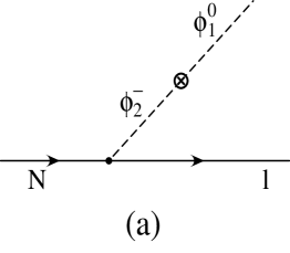
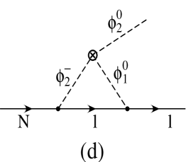
Figure 1: Diagrams which contribute, up to one-loop order, to charge violating process $N\rightarrow l\,\phi^{0}_{1,2}$. Filled boxes (circled crosses) are used to indicate CP-even (odd) charge violating mixings or interactions between the gauge eigenstates.

Then we consider the process $N\rightarrow l\,\phi_{1,2}^{0}$, presented in Fig. 1, and for simplicity we assume one family. In order to calculate the net electric charge production rate we compare, as in the case of baryon asymmetry [17, 46], the decay rate of process $N\rightarrow l\,\phi_{1,2}^{0}$ and that of its CP conjugate. The difference of these rates will be proportional to the produced average net electric charge. In Figs. 1,2 filled boxes (circled crosses) are used to indicate CP-even (odd) charge violating mixings or interactions between the gauge eigenstates. The circled crosses depend on the complex couplings $\mu_{3},\lambda_{6,7}$. All lines in Figs. 1,2 represent gauge eigenstates, just in order to make apparent the charge violating mixings and interactions. These gauge eigenstates are linear combinations of the corresponding mass eigenstates.

In Fig. 1a the tree level graph does depend on the CP violating complex parameter $\lambda_{7}$. In the Born approximation there is no net electric charge production, since the cross section remains invariant under the CP transformation, even if complex couplings are involved:

$$\Gamma^{{\rm Born}}(N\rightarrow l\,\phi_{1}^{0})=\Gamma^{{\rm Born}}(\overline{N}\rightarrow\overline{l}\,\phi_{1}^{0*})\,.$$ (23)

The one-loop diagram displayed in Fig. 1b depends linearly on the Yukawa coupling $h_{l}$, which can be complex in general, and on $\lambda_{3}$ which is however real. The complexity of $\lambda_{7}$ and Yukawa couplings results to non-vanishing net electric charge production from the interference term of the tree level graph in Fig. 1a and the one-loop graph in Fig. 1b. The contribution of this interference term can be written as:

$$\Gamma^{{\rm interf}}(N\rightarrow l\,\phi_{1}^{0})=\lambda_{3}h_{l}\ I_{Nl}\,\left|\left\langle{\phi_{2}^{-}}\right\rangle\right|{\lambda}_{7}{(}h_{N})^{2}+\,h.c.\,,$$ (24)

where $\,I_{Nl}$ is the relevant kinematic factor corresponding to this interference term. For simplicity we have assumed that $h_{N}$ is real. The CP dependence of these elements is of the order of the phases of $h_{l}$ and $\lambda_{7}$. The CP conjugate process $\overline{N}\rightarrow\overline{l}\,\phi_{1}^{0*}$ yields an interference contribution:

$$\Gamma^{{\rm interf}}(\overline{N}\rightarrow\overline{l}\,\phi_{1}^{0*})=\,\,\lambda_{3}h_{l}^{*}\ I_{Nl}^{*}\,\left|\left\langle{\phi_{2}^{-}}\right\rangle\right|{\lambda}_{7}^{*}{(}h_{N})^{2}+\,h.c.\,,$$ (25)

where in both Eqs. (24) and (25), we have used the modulus of $\langle\phi_{2}^{-}\rangle$ , since spontaneous CP violating phases cancel each other.

The net electric charge produced during the first stage of the phase transition through the process $N\rightarrow l\,\phi_{1}^{0}$ is proportional, at the one-loop order, to the quantity

$$\Gamma^{{\rm interf}}(N\rightarrow l\,\phi_{1}^{0})-\Gamma^{{\rm interf}}(\overline{N}\rightarrow\overline{l}\,\phi_{1}^{0*})\simeq 4\,\lambda_{3}\,\left|\left\langle{\phi_{2}^{-}}\right\rangle\right|\,{\mathop{\rm Im}}[h_{l}{\lambda}_{7}]\ \mathop{\rm Im}[\ I_{Nl}]\,h_{N}^{2}.$$ (26)

To leading order, in the small CP violating phases, the following approximation holds

$$\,{\mathop{\rm Im}}[h_{l}{\lambda}_{7}]\ \simeq\left|{\lambda}_{7}\right|\left|h_{l}\right|\left(\theta_{7}+{\arg}(h_{l})\right)\,.$$ (27)

The average net electric charge produced via the above charge violating process, measured in units of the electron charge, is therefore

$$\Delta Q={\ \frac{1}{{\Gamma}_{N}}}\left[\Gamma^{{\rm interf}}(N\rightarrow l\,\phi_{1}^{0})-\Gamma^{{\rm interf}}(\overline{N}\rightarrow\overline{l}\,\phi_{1}^{0*})\right]\,,$$ (28)

where ${\Gamma}_{N}\simeq\frac{h_{N}^{2}}{8\pi}M$. Using Eq. (26), Eq. (28) can take the form

$$\Delta Q\simeq{\frac{32\pi\lambda_{3}}{M}}\,\,\left|\left\langle{\phi}_{2}^{-}\right\rangle\right|\left|{\lambda}_{7}\right|\,\,\left|h_{l}\right|\left(\theta_{7}+{\arg}(h_{l})\right)\,{\mathop{\rm Im}}\left[I_{Nl}\right]\,.$$ (29)

For the process $N\rightarrow l\,\phi_{2}^{0}$, presented in Fig. 1c-1d, we get a similar contribution to $\Delta Q$ with $\lambda_{3}$ replaced by $\lambda_{2}$. So the net charge density produced during the charge violating phase, if all the CP violating phases are of order $10^{-4}$ as required by baryogenesis scenarios, turn out to be

$$\Delta Q\simeq\frac{10^{-8}}{M/\;\mathrm{TeV}}\,,$$ (30)

leading to

$$n_{Q}/s\simeq\frac{\Delta Q\,\ n_{{\rm N}}}{g_{*}\,n_{\gamma}}\simeq\left(\frac{10^{-8}}{M/\;\mathrm{TeV}}\right)\frac{n_{{\rm N}}}{g_{*}\,n_{\gamma}}.$$ (31)

For $M=1\;\mathrm{TeV}$, $\frac{n_{{\rm N}}}{g_{*}\,n_{\gamma}}\simeq 10^{-5}$, yielding $n_{Q}/s\simeq 10^{-13}$ which is clearly much larger than the bounds $10^{-29}$–$10^{-30}$ quoted previously. However the heavy neutrino density $n_{{\rm N}}$ falls rapidly with increasing $M$ resulting to a smaller charge asymmetry. In order to find $n_{{\rm N}}$ at the electroweak scale $T=100\;\mathrm{GeV}$ one has to solve the appropriate Boltzmann equation. By solving this, we find that the bound $10^{-30}$ on $n_{Q}/s$ is saturated for a mass $M\approx 5\;\mathrm{TeV}$. For larger values of $M$ the aforementioned upper bound on $n_{Q}/s$ is always satisfied. Thus in such models the cosmological upper limits on the charge asymmetry impose lower bounds on the heavy neutrino masses, unless the combination of phases appearing in Eq. (29) is fine tuned to values much smaller than $10^{-4}$.

There are also other charge violating processes $N\rightarrow l\,V$ ($V$ denotes the neutral gauge bosons) that can produce charge asymmetry through the interference of the tree-level graph, presented in Fig. 2, with the corresponding one-loop graphs. This process is less significant than the one we considered above since its rate is $\frac{M_{w}}{M}$ times smaller than the rate of the previous interaction. However if $\theta_{7}={\arg}(h_{l})=0$ then the process $N\rightarrow l\,V$ is the dominant mechanism for charge asymmetry provided $\theta_{3}$, $\theta_{6}$ are different from zero. When the the Yukawa coupling $h_{N}$ of the heavy leptons is complex, the process $N\rightarrow l\,\phi_{1,2}^{0}$ can lead to non-zero charge asymmetry if we adopt the model of Ref. [45] and use a similar interference pattern with that presented in Ref. [47].

To summarize, in this paper we discuss the phase transition of a model with two Higgs doublets, in which CP violating terms are present in the scalar potential. The motivation for this study originates from the fact that the successful mechanisms for explaining baryogenesis are based on such models. Besides this, such an extended Higgs sector resembles that of supersymmetric (SUSY) models and hence our conclusions may be of relevance for SUSY extensions of the SM.

Using the finite temperature one-loop corrected effective potential we found that the phase transition occurs in two stages. During the first stage of the transition CP violating angles are amplified, as required by baryogenesis, and simultaneously a charge breaking stationary point is developed which is a minimum, in a wide range of the parameter space. This leads to a non-vanishing charge asymmetry, in the presence of heavy leptons, due to the appearance of CP violating sources within the $D-$breaking terms and/or Yukawa couplings. In the context of the SM no net charge asymmetry is produced. However in models with heavy leptons the magnitude of the asymmetry is found to exceed existing astrophysical bounds, constraining the mass spectrum of heavy leptons. In particular in models with heavy neutrinos we find that heavy neutrino masses smaller than $5\;\mathrm{TeV}$ result to unacceptably large charge asymmetry.

The study undertaken in this paper maybe of relevance for supersymmetric models and other extensions of the SM which are characterized by a complicated Higgs sector and CP violating sources in the SUSY breaking terms of the scalar potential. The development of a charge breaking minimum during the cooling down of the Universe may lead, in this case too, to a large net charge asymmetry restricting the allowed parameter space. Besides this, one has to pay special attention to the appearance of other kinds of minima, such as color breaking, which develop at finite temperatures. These may impose further constraints on supersymmetry parameters and affect the phenomenological predictions. Such a study is under consideration and the results will appear elsewhere.

It is worth mentioning that the possible two stage transition, studied in this paper, may be a feature shared by other multiscalar potentials deserving special attention. In GUT theories the breaking of $U(1)_{em}$ symmetry at the unification scale offers a working mechanism for the resolution of the monopole problem as proposed by Langacker and Pi [48].

Acknowledgments

We would like to thank T.W.B. Kibble and N. Tetradis for helpful discussions. Our thanks are also due to A. Pilaftsis for useful comments and suggestions. A.B.L. acknowledges support from ERBFMRXCT–960090.

Table 1: Sample of allowed parameters respecting all theoretical constraints and experimental bounds on Higgs boson masses (see main text).

$\lambda_{1}/g^{2}$	$\lambda_{2}/g^{2}$	$\lambda_{3}/g^{2}$	$\lambda_{4}/g^{2}$	$\lambda_{5}/g^{2}$
1.0	1.0	1.0	–1.0	–1.0
1.0	1.0	–0.1	–1.0	–0.1
1.0	1.0	0.1	–1.0	–0.1
1.0	1.0	1.0	–1.0	–0.1
1.0	1.0	–0.1	0.1	–1.0
1.0	1.0	0.1	0.1	–1.0
1.0	1.0	1.0	0.1	–1.0

Figure 2: Tree level diagrams which contribute to charge violating process $N\rightarrow l\,V$. The filled box is as in Fig. 1.

References

- [1] A.D. Sakharov, Pis’ma Zh. Eksp. Teor. Fiz. 5 (1967) 32.
- [2] M.B. Gavela, P. Hernandez, J. Orloff, O. Pene and C. Quimbay, Nucl. Phys. B430 382 (1994).
- [3] T.D. Lee, Phys. Rev. D8 (1973) 1226; Phys. Rep. 96 (1974) 143.
- [4] G. Branco, Phys. Rev. D22 (1980) 2901.
- [5] G. Branco, and M. Rebelo, Phys. Lett. B160 (1985) 117.
- [6] J. Liu and L. Wolfenstein, Nucl. Phys. B289 (1987) 1.
- [7] M. Shaposhnikov, JETP Lett. 44 (1986) 465.
- [8] L. McLerran, Phys. Rev. Lett. 62 (1989) 1075.
- [9] N. Turok and N.J. Zadrozny, Phys. Rev. Lett. 65 (1990) 2331; Nucl. Phys. B358 (1991) 471.
- [10] M. Dugan, B. Grinstein and L. Hall, Nucl. Phys. B25 (1985) 413.
- [11] T. Falk and K.A. Olive, hep-ph/9806236.
- [12] T. Ibrahim and P. Nath, hep-ph/9807501.
- [13] M. Brhlik, G.J. Good and G.L. Kane, hep-ph/9810457.
- [14] D. Chang, W.-Y. Keung and A. Pilaftsis, Phys. Rev. Lett. 82 (1999) 900.
- [15] S. Weinberg, Phys. Rev. Lett. 37 (1976) 657.
- [16] A.B. Lahanas and C.E. Vayonakis, Phys. Rev. D19 (1979) 2158.
- [17] A. Riotto, Lectures at Summer School in High Energy Physics and Cosmology, ICTP Miramare-Trieste, July 1998, hep-ph/9807454.
- [18] D. Land and E.D. Carlson, Phys. Lett. B292 (1992) 107.
- [19] V. Zarikas, Phys. Lett. B384 (1996) 180.
- [20] D. Comelli, M. Pietroni and A. Riotto, Nucl. Phys. B412 (1994) 441.
- [21] D. Comelli and M. Pietroni, Phys. Lett. B306 (1993) 67.
- [22] M. Gell-Mann, P. Ramond and R. Slansky, in “Supergravity”, ed. P. van Nieuwenhuizen and D. Freedman, North Holland 1979, p. 315.
- [23] T. Yanagida, Prog. Theor. Phys. 4 (1980) 1103.
- [24] A. Pilaftsis, Z. Phys. C55 (1992) 275.
- [25] L.N. Chang, D. Ng and J.N. Ng, Phys. Rev. D50 (1994) 4589.
- [26] A. Dolgov and J. Silk, Phys. Rev. D47 (1993) 3144.
- [27] M. Sher, Phys. Rep. 179 (1989) 273.
- [28] T.W.B. Kibble, in “Topology of cosmic domains and strings”, J. Phys. A: Math. Gen. 9 (1976) 1387.
- [29] J.M. Cline, K. Kainulainen and A.P. Vischer, Phys. Rev. D54 (1996) 2451.
- [30] J.M. Moreno, M. Quiros and M. Seco, hep-ph/9801272.
- [31] M. Laine and K. Rummukainen, Phys. Rev. Lett. 80 (1998) 5259.
- [32] L. Dolan and R. Jackiw, Phys. Rev. D9 (1974) 3320.
- [33] N. Goldenfeld, in Proc. NATO ARW on “Formation and Interactions of Topological Defects”, A.C. Davis and R.H. Brandeberger (eds), Plenum Press, New York 1995.
- [34] T. Tanaka, M. Sasaki and K. Yamamoto, Phys. Rev. D49 (1994) 1039.
- [35] M. Dine, R.G. Leigh, P. Huet, A. Linde and D. Linde, Phys. Rev. D46 (1992) 550.
- [36] A. Strumia and N. Tetradis, Nucl. Phys. B542 (1999) 719.
- [37] I. Moss and V. Zarikas, preprint NCL95-TP5.
- [38] M. Joyce, T. Prokopec and N. Turok, Phys. Rev. D53 (1996) 2930; Phys. Rev. D53 (1996) 2958.
- [39] R.A. Lyttleton and H. Bondi, Proc. Roy. Soc. (London) A252 (1959) 313.
- [40] S. Sengupta and P.B. Pal, Phys. Lett. B365 (1996) 175; Erratum B390 (1997) 450.
- [41] S. Orito and M. Yoshimura, Phys. Rev. Lett. 54 (1985) 2457.
- [42] I. Melo, Ph.D. Thesis, Carleton Univ., Ottawa-Ontario, February 1996, hep-ph/9612488.
- [43] D. Wyler and L. Wolfenstein, Nucl. Phys. B218 (1983) 205; E. Witten, Nucl. Phys. B268 (1986) 79; R.N. Mohapatra and J.W.F. Valle, Phys. Rev. D34 (1986) 1642; S. Nandi and U. Sarkar, Phys. Rev. Lett. 56 (1986) 564; A.S. Joshipura and U. Sarkar, Phys. Rev. Lett. 57 (1986) 33.
- [44] P. Kalyniak and I. Melo, Phys. Rev. D55 (1997) 1453.
- [45] A. Pilaftsis, Phys. Rev. D56 (1997) 5431; Int. J. Mod. Phys. A14 (1999) 1811.
- [46] E.W. Kolb and M.S. Turner, “The Early Universe”, Addison-Wesley, New York 1990.
- [47] M. Fukugita and T. Yanagida, Phys. Lett. B174 (1986) 45.
- [48] P. Langacker and S. -Y. Pi, Phys. Rev. Lett. 45 (1980) 1.