Microwave background anisotropies in quasiopen inflation

Abstract

Quasiopenness seems to be generic to multi-field models of single-bubble open inflation. Instead of producing infinite open universes, these models actually produce an ensemble of very large but finite inflating islands. In this paper we study the possible constraints from CMB anisotropies on existing models of open inflation. The effect of supercurvature anisotropies combined with the quasiopenness of the inflating regions make some models incompatible with observations, and severely reduces the parameter space of others. Supernatural open inflation and the uncoupled two-field model seem to be ruled out due to these constraints for values of $\Omega_{0}\lesssim 0.98$. Others, such as the open hybrid inflation model with suitable parameters for the slow roll potential can be made compatible with observations.

]

I Introduction

There is at present some evidence, based on observations of supernovae at large redshift [1], that the Universe may not be Einstein-deSitter ($\Omega_{\rm m}=1,\ \Omega_{\Lambda}=0$), as predicted by the simplest models of inflation. Furthermore, recent observations of the microwave background (CMB) and large scale structure indicate that the Universe may be open ($\Omega_{0}=\Omega_{\rm m}+\Omega_{\Lambda}=0.8\pm 0.3$)[2]. In the near future, observations of the microwave background with a new generation of satellites, MAP and Planck, will determine with an accuracy of order 1% whether we live in an open Universe or not. It is therefore crucial to know whether inflation can be made compatible with such a Universe.

The idea that the Universe might be open is an old one, see for instance [3]. Early attempts to accommodate standard inflation in an open Universe failed to realize the fact that, in usual inflation, homogeneity implies flatness [4], because of the Grishchuck–Zel’dovich effect [5]. The possibility of having, through the nucleation of a single bubble in de Sitter space, a truly open Universe arising from inflation is not new either, see [6, 7]. However, a concrete realization of a fully consistent model was suggested only recently, the single-bubble open inflation model [8, 9]. Since then, there has been great progress in determining the precise primordial spectra of perturbations [10, 11, 12, 13, 14, 15, 16, 17, 18, 19, 20, 21, 22, 23], most of it based on quantum field theory in spatially open spaces. Simultaneously, a large effort was made in model building [9, 24, 25, 26] and in constraining the existing models from observations of the temperature power spectrum of CMB anisotropies [25, 26, 27, 28].

Open inflation models provide a natural scenario for understanding the large-scale homogeneity and isotropy. Furthermore, these inflationary models generically predict a nearly scale-invariant spectrum of density and gravitational wave perturbations, which could be responsible for the observed CMB temperature anisotropies. Future precise observations could determine whether indeed these models are compatible with the observed features of the CMB power spectrum. For that purpose it is necessary to know the predicted spectrum with great accuracy. As we will show, open models have a more complicated primordial spectrum of perturbations, with extra discrete modes and possibly large tensor anisotropies.

The simplest inflationary model consistent with an open Universe arises from the nucleation of a bubble in de Sitter space [6], inside which a second stage of inflation drives the spatial curvature to almost flatness. The small deviation from flatness at the end of inflation will be amplified by the subsequent expansion during the radiation and matter eras. The present value of the density parameter is determined from $(1-\Omega_{0})/\Omega_{0}\sim\exp(-2N_{e})\times 10^{54}$, where $N_{e}\leq 60$ is the required number of $e$-folds during inflation (inside the bubble), in order to give an open Universe today. A few percent change in $N_{e}$ could lead to an almost flat Universe or to a wide open one.

This simple picture could be realized in the context of a single-field scalar potential [8] or in multiple-field potentials [9, 24, 25, 26], as long as there exists a false vacuum epoch during which the Universe becomes homogeneous and then one of the fields tunnels to the true vacuum, creating a single isolated bubble. The space-time inside this bubble is that of an open Universe [29, 6]. Although single-field models can in principle be constructed, they require a certain amount of fine-tuning in order to avoid tunneling via the Hawking–Moss instanton [9]. The problem is that a large mass is needed for successful tunneling and a small mass for successful slow-roll inside the bubble. For that reason, it seems more natural to consider multiple-field models of open inflation [9, 24, 25, 26], where one field does the tunneling, another drives slow-roll inflation inside the bubble, and yet another may end inflation, as in the open hybrid model [26]. Such models account for the large-scale homogeneity observed by COBE [30] and are also consistent with recent determinations of a small density parameter [31, 32, 33, 34].

In this paper, we shall systematically explore the possible constraints from CMB anisotropies on existing models of open and quasiopen inflation. The structure of the paper is as follows. In sections II and III, a brief review of the quantum tunneling and the primordial spectrum of perturbations is given. Section IV is devoted to quasiopen inflation. In section V some general bounds are found from CMB observations. In section VI, the bounds derived in the previous section are used to constrain several models of open inflation. Section VII discusses the probability distribution for $\Omega_{0}$ in quasi-open inflation and corresponding constraints on the parameters of the models. Section VIII contains our conclusions.

II Quantum tunneling

The quantum tunneling that gives rise to the single bubble of open inflation can be described with the use of the bounce action formalism developed by Coleman–DeLuccia [29] and by Parke [35] in the thin-wall approximation, valid when the width of the bubble wall is much smaller than the radius of curvature of the bubble. This only requires that the barrier between the false and the true vacuum be sufficiently high, $U_{0}\gg\Delta U=U_{F}-U_{T}$. In this case we can write the radius of the bubble in terms of the dimensionless parameters $a$ and $b$ [28],

$$R_{0}H_{T} = [1+(a+b)^{2}]^{-1/2}\equiv[1+\Delta^{2}]^{-1/2}\,,$$ (2)

$$a\equiv{\Delta U\over 3S_{1}H_{T}},\hskip 28.45274ptb\equiv{\kappa^{2}S_{1}\over 4H_{T}}\,,$$

where $\kappa^{2}\equiv 8\pi G$ and $S_{1}$ is the surface tension of the bubble wall, computed as $S_{1}=\int_{\sigma_{F}}^{\sigma_{T}}d\sigma\,[2(U(\sigma)-U_{F})]^{1/2}$. Here $\sigma$ is the tunneling field. Since $S_{1}\sim U_{0}/M\sim M(\Delta\sigma)^{2}$ for a mass $M$ in the false vacuum, the parameter $a\simeq(\Delta U/U_{0})\,M/H_{T}$, which characterizes the degeneracy of the vacua, can be made arbitrarily small by tuning $U_{T}\simeq U_{F}$. On the other hand, the parameter $b\simeq(\Delta\sigma/M_{\rm Pl})^{2}M/H_{T}$, which characterizes the width of the barrier, is not so easily tunable, and could be very large or very small depending on the model.

In order to prevent collisions with other nucleated bubbles (at least in our past light cone) it is necessary that the probability of tunneling be sufficiently suppressed. For an open Universe of $\Omega_{0}>0.2$, this is satisfied as long as the bounce action $S_{B}>6$, see Ref. [6]. This imposes only a very mild constraint on the tunneling parameters $a$ and $b$, as long as the energy density in the true vacuum satisfies $U_{T}\ll M_{\rm Pl}^{4}$, see Ref. [28].

III Primordial perturbation spectra

There are essentially two kinds of primordial perturbations in open inflation, subcurvature and supercurvature. In the first category we have the usual scalar and tensor metric perturbations [11, 12, 18], which are generated during the slow roll inflation inside the bubble. The second category of modes arises because of perturbations which are generated outside the bubble or as a result of the acceleration of the expanding bubble [10, 27, 12]. In particular, the fluctuations of the bubble wall itself generate perturbations [14, 15, 16, 19] which are specific to open inflation. In addition, in the context of two-field models of open inflation [9], we have semi-classical effects due to tunneling to different values of the inflaton field [20, 21]. All these perturbations create anisotropies in the CMB, which distort the angular power spectrum on large scales (low multipoles). On smaller scales, the particle horizon at last scattering subtends an angle of about one degree on the sky for a flat universe, and somewhat smaller for an open universe, due to the projection effect of the geodesics. This effect shifts the first acoustic peak of the temperature power spectrum to higher multipoles ($l_{\rm peak}\sim 208\ \Omega_{0}^{-1/2}$) [36, 37], but the primordial spectrum at those multipoles is essentially that of a flat Universe.

A Subcurvature scalar and tensor perturbations

Soon after the proposal of a single-bubble open inflation model [8], the primordial spectrum of scalar perturbations was computed and found to be identical to that of the flat case, except for a prefactor that depends on the bubble geometry [12],

$${\cal P}_{\cal R}(q)=A_{S}^{2}\,f(q)\,,\hskip 28.45274ptA_{S}^{2}={\kappa^{2}\over 2\epsilon}\Big{(}{H_{T}\over 2\pi}\Big{)}^{2}\,.$$ (3)

Here ${\cal P}_{\cal R}(q)$ is the primordial spectrum of scalar metric perturbations ${\cal R}$, in term of which the continuum part of the power spectrum is written as

$$\langle|{\cal R}(q)|^{2}\rangle={2\pi^{2}{\cal P}_{\cal R}(q)\over q(1+q^{2})}\,.$$ (4)

The function $f(q)$ [12] depends on the tunneling parameters $a$ and $b$, see Eq. (2),

$$f(q)=\coth\pi q-{z^{2}\cos\tilde{q}+2qz\sin\tilde{q}\over(4q^{2}+z^{2})\,\sinh\pi q}\,,$$ (5)

where $\tilde{q}=q\ln((1+x)/(1-x))$ and

$$x = (1-R_{0}^{2}H_{T}^{2})^{1/2}=\Delta\,(1+\Delta^{2})^{-1/2}\,,$$ (6)

$$z = (1-R_{0}^{2}H_{T}^{2})^{1/2}-(1-R_{0}^{2}H_{F}^{2})^{1/2}$$ (7)

$$= 2b\,(1+\Delta^{2})^{-1/2}\,,$$ (8)

see Eq. (2). The function $f(q)$ is linear at small $q$, and approaches a constant value $f(q)=1$ at $q\geq 2$. Here $q$ is the effective momentum for scalar modes in an open Universe, determined from $q^{2}=k^{2}-1$, where $-k^{2}$ is the eigenvalue of the Laplacian. For scalar perturbations, the effect of $f(q)$ on the temperature power spectrum is almost negligible, and therefore the tilt of the scalar spectrum is approximately given by the same formula as in flat space [38]:

$$n_{S}-1\equiv{d\ln{\cal P}_{\cal R}(k)\over d\ln k}\simeq-6\epsilon+2\eta\,,$$ (9)

in the slow-roll approximation,

$$\epsilon={1\over 2\kappa^{2}}\,\Big{(}{V^{\prime}(\phi)\over V(\phi)}\Big{)}^{2}\ll 1\,,\hskip 22.76219pt\eta={1\over\kappa^{2}}\,{V^{\prime\prime}(\phi)\over V(\phi)}\ll 1\,.$$ (10)

On the other hand, the primordial spectrum of tensor or gravitational waves anisotropies took much longer to evaluate. For some years, there seemed to be a problem with the power spectrum of tensor anisotropies, which presented an infrared divergence at $q=0$ in an open Universe [39]. It was clear that a physical regulator was necessary. But this is precisely the role played by the bubble wall; recent computations have shown that in the presence of the bubble the tensor primordial spectrum* ‣ III A is given by [18]

$$\langle|h(q)|^{2}\rangle=\frac{\pi^{2}{\cal P}_{g}(q)}{4q(1+q^{2})}\,,$$ (11)

where

$${\cal P}_{g}(q)=A_{T}^{2}\,f(q)\,,\hskip 28.45274ptA_{T}^{2}=8\kappa^{2}\Big{(}{H_{T}\over 2\pi}\Big{)}^{2}\,.$$ (12)

It is the shape of the function $f(q)$, see Eq. (5), that gives a finite physical observable, as we will explain in Section V A. Here $q$ is the effective momentum for tensor modes, defined by $q^{2}=k^{2}-3$. While for scalar modes the presence of this function $f(q)$ in the primordial spectrum becomes irrelevant for observations, for tensor modes the slope of the function at $q=0$ is an important ingredient in the final value of the predicted power spectrum at low multipoles [28].

Note that the above spectra have been obtained under the small backreaction approximation. Immediately after nucleation, the scalar and tensor modes have been assumed to evolve in a nearly de Sitter spacetime. This assumption is reasonably fulfilled in the models considered in this paper, but in models where the inflaton moves initially very fast, the infrared end of the spectrum may be slightly different[23].

B Supercurvature and bubble-wall modes

Apart from the usual continuum ($q^{2}\geq 0$) of scalar and tensor modes, generalized to an open Universe, in single-bubble inflationary models there is a new type of quantum fluctuations, which basically account for the combined effect of fluctuations generated during the false vacuum dominated era which penetrate the bubble, as well as excitations of the slow roll field generated by the accelerated growth of the bubble. These modes are discrete modes, which appear in particular when the mass of the scalar field in the false vacuum is smaller than the rate of expansion, $m^{2}<2H^{2}$. The supercurvature mode was first postulated in Ref. [10], from purely mathematical arguments related to homogeneous Gaussian random fields in spatially open universes. Only later did concrete models of single-bubble open inflation [11, 12] show its existence in the primordial spectrum of scalar fluctuations. These modes are characterized by having an imaginary effective momentum (or equivalently, $k^{2}<1$), and therefore describe fluctuations over scales larger than the curvature scale, whence its name of supercurvature mode [remember than the curvature scale corresponds to the eigenmode with eigenvalue $k^{2}=1,\ q^{2}=0$].

The amplitude of the supercurvature mode (for the usual two-field models like the ones described by (65), see below) is found to be[12, 27] * ‣ III A

$$\langle|{\cal R}_{\Lambda}|^{2}\rangle=\pi^{2}A_{SC}^{2}\,,$$ (13)

where

$$A^{2}_{SC}={\kappa^{2}\over\epsilon}\,\Big{(}{H_{F}\over 2\pi}\Big{)}^{2}=A^{2}_{S}\,{2H_{F}^{2}\over H_{T}^{2}}\,,$$ (14)

whith $A^{2}_{S}$ given by Eq. (3).

However, this is not the only discrete supercurvature mode possible in single-bubble models. As realized in Refs. [13, 14, 15], there are also scalar fluctuations of the bubble wall with $k^{2}=-3,\ q^{2}=-4$, which could in principle have its imprint in the CMB anisotropies. Their amplitude was computed in Refs. [15, 16], based on field theoretical arguments:

$$\langle|{\cal R}_{W}|^{2}\rangle=4\pi^{2}A_{W}^{2}\,.$$ (15)

Here

$$A^{2}_{W}={\kappa^{2}\over 2z}\,\Big{(}{H_{T}\over 2\pi}\Big{)}^{2}=A_{S}^{2}\,{\epsilon\over z}\,,$$ (16)

where $z$ is given by Eq. (8) and $A^{2}_{S}$ is the scalar amplitude (3). Such modes contribute as transverse traceless curvature perturbations [15, 14], which nevertheless behave as a homogeneous random field [17]. It was later realized [19] that the bubble-wall fluctuation mode is actually part of the tensor primordial spectrum, once the gravitational backreaction is included, so we should not consider it as a new source of anisotropies if the tensor mode is properly taken into account.

IV Quasiopen inflation

All single-field models of open inflation predict the above primordial spectra of anisotropies: a continuum of scalar and tensor modes and the (possible) discrete supercurvature modes. However, as mentioned in the introduction, it is difficult to construct such models without a certain amount of fine-tuning [9], and thus multiple-field models were considered [9, 24, 25, 26]. In these models, one field $\sigma$ would do the tunneling while inside the bubble a second field $\phi$ would drive slow-roll inflation. However, a large class of two-field models do not lead to infinite open Universes, as was previously thought, but to an ensemble of very large but finite inflating ‘islands’. The most probable tunneling trajectory corresponds to a value of the inflaton field at the bottom of its potential; large values, necessary for the second period of inflation inside the bubble, only arise as localized fluctuations. These fluctuations are provided precisely by the supercurvature modes of the slow-roll field $\phi$, which due to their long wavelength can create large regions of size larger than the hubble radius where the field is coherent and thus can drive inflation. The interior of each nucleated bubble will contain an infinite number of such inflating regions of co-moving size of order $\gamma^{-1}$, where $\gamma\ll 1$ is given by the supercurvature eigenvalue $\gamma=1+q^{2}\equiv 1-\Lambda^{2}$ (this in turn depends on the parameters of the model, see below). We may happen to live in one of those patches of co-moving size $d\leq\gamma^{-1}$, where the Universe appears to be open. This scenario was recently discussed in Ref. [21]. Here we will give a brief account of the main results.

After tunneling in the $\sigma$-field direction, there remains in the $\phi$-field (inflaton) direction a semiclassical displacement characterized by a Gaussian distribution with r.m.s. amplitude $f$, where

$$f^{2}\equiv\langle\phi^{2}(t_{0})\rangle\approx{H_{F}^{2}\over(2\pi)^{2}\gamma}$$ (17)

If $f$ is sufficiently large (for a power law potential this means $f\sim M_{\rm Pl}$, whereas for the open hybrid model [26], a much smaller $f$ would do), then the fluctuations of the field $\phi$ will make inflation generic inside the bubble. However, regions of size $r\sim\gamma^{-1}$ with large positive $\phi$ will be separated from regions with large negative $\phi$ by non-inflating regions where $\phi$ is small.

In many models, however, the r.m.s. fluctuation $f$ is much smaller than the field value needed for inflation. Then, most of the hypersurface $t=t_{0}\sim H^{-1}$ inside the bubble will not be inflating, leading to empty space with no galaxies. On the other hand, inflating regions will still arise as localized “rare” fluctuations, with exponentially suppressed probability

$$P\propto\exp(-\phi^{2}/2f^{2}),$$ (18)

where $\phi\sim M_{\rm Pl}$. High peaks of a random Gaussian field tend to be spherical. If we choose the origin of coordinates on the $t=const$ hyperboloid to be at the center of the island, then the profile of the field as we move outwards is given by the $l=0$ supercurvature mode [see Equation (A4)], normalized to the value $\phi_{c}$ at the center of the bubble [21],

$$\phi^{\gamma}_{l=0}=\phi_{c}(t){\sinh(\Lambda r)\over\Lambda\sinh r}.$$ (19)

The r.m.s. amplitude of the remaining $l>0$ supercurvature modes, which would account for departures from sphericity, is much smaller, of order $\gamma^{1/2}f\ll f\ll\phi(t_{0})$.

Let us concentrate on one of these inflating regions. The initial value of $\phi_{c}$ determines how many e-foldings of inflation the center of the island will undergo, and hence the value of $\Omega_{0}$ that an observer in that region would measure after inflation, at a given CMB temperature. For the sake of illustration, let us assume that this observer measures $\Omega_{0}=0.5$ at the time when $T_{\rm CMB}=2.728$ K. Also, let us take $\gamma=10^{-4}$. For $r\ll\gamma^{-1}\sim 10^{4}$ the field on a $t=const$ slice will decrease very slowly with distance as we move away from the center. Note that at large distances from the center $r\gg 1$ we have $\phi^{\gamma}\propto\exp(-\gamma r/2)$. Denoting by $N$ the number of e-foldings of inflation and assuming a quadratic potential (a similar argument can be made for the hybrid model), we have $\delta N/N\approx 2\delta\phi/\phi$. Using the relation $2\delta N=[\Omega_{0}(\Omega_{0}-1)]^{-1}\delta\Omega_{0}$, we find that observers out to a distance $r\sim 10$ would measure a very similar density parameter, which differs from the one at the center only by $\delta\Omega_{0}\approx\Omega_{0}(\Omega_{0}-1)N\gamma r\lesssim 10^{-2}$. On the other hand, for $r\sim\gamma^{-1}=10^{4}$ the universe will look rather empty, and even if inflation proceeds there for a few e-foldings, the density parameter would be too low for any galaxies to form and for observers to develop.

Although the inflating region in the example above has spherical symmetry around $r=0$, it is clear that most observers in that island will live at $r\gg 1$. To them the universe would look anisotropic. This effect was dubbed “classical anisotropy” [20], and can be estimated as follows. After expansion of (19) for $r\ll\gamma^{-1}$, we can separate the $t$-dependent background from the $t$ and $r$ dependent perturbation, $\phi^{\gamma}_{l=0}=\phi_{c}(t)+\delta\phi$, where

$$\delta\phi=\phi_{c}(t){\gamma\over 8}(1-4r\coth r)\approx-\phi_{c}(t){\gamma\over 2}\ln\cosh r\,,$$ (20)

the last expression being a very good approximation for $1\ll r\ll\gamma^{-1}$. To describe the Universe from the point of view of an observer living at $r=r_{0}\gg 1$, it is convenient to change the coordinates $(r,\theta,\phi)$ on the spacelike hyperboloid to a new set $(r^{\prime},\theta^{\prime},\phi^{\prime})$ such that the point $r=r_{0}$ is now the new origin of coordinates, $r^{\prime}=0$. In that case, we have $\cosh r=\sinh r_{0}\sinh r^{\prime}\cos\theta^{\prime}+\cosh r_{0}\cosh r^{\prime}$, and the field can be separated in the form $\phi^{\gamma}_{l=0}=\phi_{0}(t)+\delta_{0}\phi$, where $\phi_{0}\approx\phi_{c}(1-\gamma r_{0}/2)$ is the value of the field at the location $r_{0}$, which corresponds to a somewhat lower value of $\Omega_{0}$ than that of the central region, and

$$\delta_{0}\phi\approx\phi_{0}(t)(\gamma/2)\ln f(r^{\prime},\theta^{\prime}),$$ (21)

with

$$f(r,\theta)\equiv\cosh r+\sinh r\,\cos\theta\,.$$ (22)

We can now evaluate the gauge invariant metric perturbation associated with this field fluctuation, which will remain constant outside the horizon and will reenter during the matter era with an amplitude

$$\Phi={3\over 5}\,{H_{T}\delta\phi\over\dot{\phi}_{0}}={3\over 5}\,A_{C}\,\ln f(r,\theta)\,,$$ (23)

where

$$A_{C}={3\over 2}{H_{T}^{2}\over m_{T}^{2}}\,\gamma\,;\ \ \gamma={2\over 3}{m_{F}^{2}\over H_{F}^{2}}+{1\over 8}H_{F}^{2}R_{0}^{4}(m_{T}^{2}-m_{F}^{2})\,.$$ (24)

Here $R_{0}$ is the radius of the bubble at tunneling (2), $m_{F}$ and $m_{T}$ are respectively the masses of the inflaton field in the false and in the true vaccuum, and $\gamma$ was computed, to order $(H_{F}R_{0})^{4}$, in Ref. [21]. Note that in the case of the simplest (uncoupled) two-field model [9], where $m_{T}=m_{F}$, these expressions coincide with those given in Ref. [20].

In deriving (21) we have concentrated in a single island and we have assumed that we live far from the center, at $r\gg 1$. This seems to be a minimal “Copernican” requirement, since in any island there are many more observers far from the center than near it. Hence, we should (at least) impose the constraint that the CMB anisotropy induced by (23) should not exceed the observational bounds.

However, this is not the full story [22]. Let us note, first of all, that the amplitude of the perturbation (21) is proportional to $\phi_{0}$. Now, when the ensemble of all possible islands that contain a particular value of $\phi_{0}$ is considered, one finds that those values of $\phi_{0}$ for which (21) would be larger than the perturbation caused by the usual supercurvature modes will occur typically near the center of the islands (see Appendix B). Hence, those are rather unlikely values of $\phi_{0}$ for us to observe. Therefore it seems reasonable to impose not only that the anisotropy (23) should not exceed the observational bounds, but also that it should not exceed the anisotropy created by the $l>0$ supercurvature modes.

These considerations naturally lead to the question of what are the most likely values for $\phi_{0}$ or what is the most probable value of $\Omega_{0}$ in a given model. The probability distribution for $\Omega_{0}$ in models of quasiopen inflation was studied in Ref. [22]. Stronger constraints on the models can be obtained from this probability distribution in combination with CMB constraints. These will be discussed in Section VII.

V CMB temperature anisotropies

Quantum fluctuations of the inflaton field $\phi$ during inflation produce long-wavelength scalar curvature perturbations and tensor (gravitational waves) perturbations, which may leave their signature in the CMB temperature anisotropies, when they re-enter the horizon. Temperature anisotropies are usually given in terms of the two-point correlation function or power spectrum $C_{l}$, defined by an expansion in multipole number $l$. We are mainly interested in the large-scale (low multipole number) temperature anisotropies since it is there that gravitational waves and the discrete modes could become important. After $l\sim 50$, the tensor power spectrum drops down [40, 41] while the density perturbation spectrum increases towards the first acoustic peak, see Ref. [42]. On these large scales the dominant effect is gravitational redshift via the Sachs–Wolfe effect [43].

A Scalar and tensor anisotropies

The Sachs-Wolfe effect for scalar perturbations with adiabatic initial conditions, like those present here, is given by [43]

$${\delta T\over T}(\theta,\phi) = {1\over 3}\Phi(0)Q(\eta_{0},\theta,\phi)$$ (25)

$$+ 2\int_{0}^{\eta_{0}}dr\,\Phi^{\prime}(\eta_{0}-r)Q(r,\theta,\phi)\,,$$ (26)

where $\eta_{0}=\cosh^{-1}(2/\Omega_{0}-1)$ is the present conformal time and, to very good approximation, also the distance to the last scattering surface ($\eta_{\rm LSS}\approx 0$). Here $Q(r,\theta,\phi)$ stands for the spatial dependence of the fluctuation [28]. The second term accounts for integration along the line of sight, and is important in an open universe, since the metric perturbation $\Phi$ evolves in time after reentering the horizon, $\Phi(\eta)=\Phi_{\rm LS}\,F(\eta)$, where $\Phi_{\rm LS}$ is the value of the perturbation at the moment of last scattering and

$$F(\eta)\equiv 5{\sinh^{2}\eta-3\eta\sinh\eta+4(\cosh\eta-1)\over(\cosh\eta-1)^{3}}\,,$$ (27)

normalized so that $F(0)=1$ at last scattering, $\eta_{\rm LSS}=0$.

One can always expand the temperature anisotropy projected on the sky in spherical harmonics,

$${\delta T\over T}(\theta,\phi)=\sum_{l=1}^{\infty}\sum_{m=-l}^{l}\,a_{lm}\,Y_{lm}(\theta,\phi)\,,$$ (28)

where the coefficients $a_{lm}$ can be obtained from

$$a_{lm}=\int d\Omega\,Y_{lm}^{*}(\theta,\phi){\delta T\over T}(\theta,\phi)\,.$$ (29)

Perturbations generated during inflation have generically Gaussian statistics since they arise from linearized quantum fluctuations. As a consequence, one can characterize the temperature anisotropies just with the two-point correlation function, or angular power spectrum,

$$\left\langle{\delta T\over T}(\hat{\bf n})\cdot{\delta T\over T}(\hat{\bf n}^{\prime})\right\rangle_{\!\!\hat{\bf n}\cdot\hat{\bf n}^{\prime}=\cos\theta}=\sum_{l=1}^{\infty}\,{2l+1\over 4\pi}\,C_{l}P_{l}(\cos\theta)\,,$$ (30)

where $(2l+1)C_{l}=\sum_{m=-l}^{l}\langle|a_{lm}|^{2}\rangle$, brackets indicating averages over different realizations.

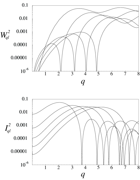
FIG. 1.: Window functions for the scalar (top figure) and tensor (bottom figure) CMB power spectra, for the first few multipoles, $l=2,4,6,8,10$ (from top-left to bottom-right), for $\Omega_{0}=0.4$. Note that the scalar window function $W_{ql}$ goes to $0$ as $q\to 0$, whereas the tensor window function $I_{ql}$ remains finite in this limit. It is for this reason that the shape of the function $f(q)$ is very important for the tensor but not much for the scalar component of temperature anisotropies.

The scalar and tensor components of the temperature power spectrum can be computed as

$$D_{l}^{S}\equiv l(l+1)C_{l}^{S} = l(l+1)\int_{0}^{\infty}dq\,\langle|{\cal R}(q)|^{2}\rangle\,W_{ql}^{2}\,,$$ (31)

$$D_{l}^{T}\equiv l(l+1)C_{l}^{T} = l(l+1)\int_{0}^{\infty}dq\,\langle|h(q)|^{2}\rangle\,I_{ql}^{2}\,,$$ (32)

where $W_{ql}$ and $I_{ql}$ [28] are the corresponding window functions ,

$$W_{ql} = {1\over 5}\Pi_{ql}(\eta_{0})+{6\over 5}\int_{0}^{\eta_{0}}drF^{\prime}(\eta_{0}-r)\Pi_{ql}(r)$$ (33)

$$I_{ql} = \int_{0}^{\eta_{0}}drG^{\prime}_{q}(\eta_{0}-r)G_{rr}^{ql}(r)\,,$$ (34)

which depend on the particular value of $\Omega_{0}$. Here, the function $G_{q}(\eta)$ is given by [18, 28]

$$G_{q}(\eta)=3\frac{\sinh\eta\sin q\eta-2q\cos q\eta(\cosh\eta-1)}{q(1+4q^{2})(\cosh\eta-1)^{2}}\,.$$ (35)

We have plotted these functions in Fig. 1 for a typical value, $\Omega_{0}=0.4$, and the first few multipoles. The scalar window functions $W_{ql}$ grow as a large power of $q$ at the origin, so that the scalar power spectrum is rather insensitive to the ‘hump’ in the function $f(q)$, as mentioned above. On the other hand, the tensor window functions $I_{ql}$ remain finite at $q=0$, and only the linear dependence of $f(q)$ at the origin prevents the existence of the infrared divergence found in [39]. Furthermore, since the functions $I_{ql}^{2}$ are not negligible near the origin, the tensor power spectrum turns out to be very sensitive to the ‘hump’ in the spectral function $f(q)$.

The ratio of tensor to scalar contribution to the temperature power spectrum is a fundamental observable in standard inflation, which depends on the slow-roll parameters (10) and provides a consistency check of the theory [38]. In single-bubble open inflation, such a ratio depends not only on the slow-roll parameters but also on the tunneling parameters (2) and on the value of $\Omega_{0}$, see Ref. [28]:

$$R_{l}={C_{l}^{T}\over C_{l}^{S}}\simeq f_{l}(\Omega_{0},a,b)\,[1-1.3(n_{S}-1)]\,16\,\epsilon\,.$$ (36)

In the ideal case in which the gravitational wave perturbation may be disentangled from the scalar component in future precise observations of the CMB power spectrum [44, 45, 46, 47, 48], it might be possible to test this relation for a given value of $\Omega_{0}$. This would constitute a check on the tunneling parameters $a$ and $b$. Such prospects are, however, very bleak from measurements of the temperature power spectrum alone, with the next generation of satellites, see e.g. [49, 45]. One can at most expect, from the absence of a significant gravitational-wave contribution to the CMB, to impose constraints on the parameters of the model. However, taking into account also the polarization power spectrum, together with the temperature data, one expects to do much better in the case of flat models, see Refs. [50, 47]. Hopefully similar conclusions can be reached in the context of open models, and CMB observations may be able to check the generalized consistency relation (36) with some accuracy.

B Supercurvature anisotropies

FIG. 2.: CMB power spectrum $l(l+1)\,C_{l}/A^{2}$, normalized to the corresponding amplitude, for the supercurvature and bubble-wall fluctuations, as a function of $\Omega_{0}$, for the first few multipoles $l=2,3,...6$ Note the dip in the supercurvature power spectrum at different values of $\Omega_{0}$ for different multipoles, due to accidental cancellations.

The supercurvature and bubble-wall modes also contribute to the temperature power spectrum. The supercurvature mode’s contribution to the CMB anisotropies can be written as

$$D_{l}^{SC}\equiv l(l+1)C_{l}^{SC}=\pi^{2}A^{2}_{SC}\,l(l+1)\bar{W}_{\Lambda,l}^{2}\,,$$ (37)

with the window function

$$\bar{W}_{\Lambda,l}={1\over 5}\bar{\Pi}_{\Lambda,l}(\eta_{0})+{6\over 5}\int_{0}^{\eta_{0}}drF^{\prime}(\eta_{0}-r)\bar{\Pi}_{\Lambda,l}(r)\,,$$ (38)

and the amplitude $A^{2}_{SC}$ is given by eq. (14)

The bubble wall mode’s contribution to the CMB anisotropies can be written as

$$D_{l}^{W}\equiv l(l+1)C_{l}^{W}=4\pi^{2}A^{2}_{W}\,l(l+1)\bar{W}_{2,l}^{2}\,,$$ (39)

where the window function is given by Eq. (38) for $\Lambda=2$, and the amplitude $A^{2}_{W}$ is found in Eq. (16)

Their contribution is plotted in Figs. 2 and 3, normalized to the corresponding amplitude, see Eqs. (14), (16) and (24), as a function of $\Omega_{0}$ for the first few multipoles. Note the dip in the spectrum at certain values of $\Omega_{0}$ due to accidental cancellations [25, 26, 28] between the intrinsic and integrated Sachs-Wolfe effects. This does not affect the bounds, since higher multipoles will fill in those gaps. The relative importance of the different components of the power spectrum is crucial in order to derive bounds on the model parameters. We have plotted in Fig. 4 the quadrupole and tenth multipole of the CMB power spectrum for each mode, normalized to their corresponding amplitudes.

C Classical anisotropies

We will concentrate here on the anisotropies associated with quasiopenness, the classical temperature anisotropies. In that case, Eq. (25) can be written as

$${\delta T\over T}(\theta) = {1\over 5}A_{C}\ln f(\eta_{0},\theta)$$ (40)

$$+ {6\over 5}\int_{0}^{\eta_{0}}dr\,F^{\prime}(\eta_{0}-r)\,A_{C}\ln f(r,\theta)\,.$$ (41)

FIG. 3.: CMB power spectrum $l(l+1)\,C_{l}^{C}$, normalized to the corresponding amplitude $A_{C}^{2}$, for the semi-classical fluctuations, as a function of $\Omega_{0}$, for the first few multipoles $l=2,3,...7$, and as a function of multipole number $l$, for $\Omega_{0}=0.3-0.9$. Note the dip in the semi-classical power spectrum at different values of $\Omega_{0}$ for different multipoles, due to accidental cancellations.

Expanding in spherical harmonics (28), we can write $a_{lm}$ as (29). In our case, since the temperature anisotropy (40) only depends on $\theta$, we find

$$a_{lm} = \left[{2l+1\over 4\pi}\right]^{1/2}\!2\pi\!\int\!d\theta\,\sin\theta\,P_{l}(\cos\theta)\,{\delta T\over T}(\theta)\ \delta_{m0}$$ (42)

$$\equiv a_{l0}\,\delta_{m0}\,.$$ (43)

It implies that the coefficients $C_{l}$ satisfy, in this case,

$$(2l+1)C_{l}^{C}=\sum_{m=-l}^{l}\langle|a_{lm}|^{2}\rangle=\langle|a_{l0}|^{2}\rangle\,.$$ (44)

Therefore, we find that the power spectrum associated with the classical anisotropies (23) can be computed as

$$D_{l}^{C} \equiv l(l+1)C_{l}^{C}=\pi\,A_{C}^{2}\,l(l+1)W_{l}^{2}\,,$$ (45)

$$W_{l} \equiv \int_{0}^{\pi}d\theta\,\sin\theta\,P_{l}(\cos\theta)\Big{[}{1\over 5}\ln f(\eta_{0},\theta)$$ (46)

$$+ {6\over 5}\int_{0}^{\eta_{0}}dr\,F^{\prime}(\eta_{0}-r)\ln f(r,\theta)\Big{]}\,.$$ (47)

We have plotted this expression in Fig. 3, as a function of multipole number $l$, for various values of $\Omega_{0}$; and as a function of $\Omega_{0}$, for the first few multipoles. As can be appreciated from the figure, the window functions for the semiclassical mode for a given $l$ are proportional to the corresponding ones for the supercurvature modes. This was expected since, as mentioned in Section IV and in Appendix B, the quasiopen island can be thought of as a superposition of supercurvature modes.

D Bounds from CMB anisotropies

From the 4-year Cosmic Background Explorer (COBE) maps [30], the overall amplitude and tilt of the CMB temperature power spectrum at small multipole number have been determined with some accuracy for $\Omega_{0}\simeq 1$ [51]

$$\left[{l(l+1)C_{l}\over 2\pi}\right]^{1/2}\! = (1.03\pm 0.07)\times 10^{-5}\,,$$ (48)

$$n = 1.02\pm 0.24\,.$$ (49)

For an open Universe, Bunn and White gave a compact expression [52]

$$A_{S} = 4.9\times 10^{-5}\,{\Omega_{0}\over g(\Omega_{0})}\,\Omega_{0}^{-0.35-0.19\ln\Omega_{0}-0.17(n_{S}-1)}$$ (51)

$$\times\exp[-(n_{S}-1)-0.14(n_{S}-1)^{2}]\,,$$

where $g(\Omega)/\Omega=5/2(1+\Omega/2+\Omega^{4/7})^{-1}$ is a fitting function to the suppression in the growth of scalar perturbations in an open universe relative to the critical density universe [53], and it was assumed that only the scalar component contributed significantly to the CMB anisotropies. Under this assumption, one can deduce the following constraints, for a scale invariant spectrum, see Refs. [28, 21],

$${H_{T}\over\sqrt{\epsilon}M_{\rm Pl}} = \sqrt{\pi}A_{S}\approx 9\times 10^{-5}\,,$$ (52)

$${H_{F}\over H_{T}} < \sqrt{\frac{D_{l}^{S}/A_{S}^{2}}{2D_{l}^{SC}/A_{SC}^{2}}}\approx 3\,,$$ (53)

$${\epsilon\over z} < \frac{D_{l}^{S}/A_{S}^{2}}{D_{l}^{W}/A_{W}^{2}}\approx 0.6\,,$$ (54)

$$A_{C} < \sqrt{\frac{D_{l}^{S}/A_{S}^{2}}{D_{l}^{C}/A_{C}^{2}}}\,A_{S}{}\approx 3\times 10^{-4}\,,$$ (55)

where the approximations are valid through the range $0.4\lesssim\Omega_{0}\lesssim 0.9$, for the quadrupole, see Fig. 5. The third expression accounts for both the tensor and the bubble-wall constraints, since the bubble-wall fluctuation is actually part of the tensor spectrum [19] and gives the largest contribution at low multipoles. The constraints coming from higher multipoles are significantly weaker, see Fig. 4. One could argue that the quadrupole is going to be hidden in the cosmic variance [48] and thus only the constraints at higher multipoles, say $l>2$, should be imposed. However, polarization power spectra may one day be used to get around cosmic variance [54] and we may be able to extract information about the scalar and tensor components at low multipoles. We will therefore take the conservative attitude that consistent models of open inflation should satisfy the bounds coming from the first few multipoles, as long as they do not exceed the associated cosmic variance.

FIG. 4.: Quadrupole (top figure) and tenth multipole (bottom figure) of the CMB power spectra, normalized to the corresponding amplitude, $l(l+1)\,C_{l}/A^{2}$, for the tensor, scalar, supercurvature, bubble-wall and semi-classical primordial spectra. We are assuming here the minimal contribution from tensors ($a=0,b=1$).

The bounds (52)-(55) are $\Omega_{0}$-dependent. For values of $(1-\Omega_{0})\ll 1$ analytic expressions for the temperature anisotropy can be found as a power series in $(1-\Omega_{0})$. In the limit $\Omega_{0}\to 1$, the scalar and the tensor contribution remain finite, whereas the supercurvature and the semiclassical anisotropies vanish, as can be seen from Fig. 4. Due to this fact, in the limit $\Omega_{0}\to 1$, the bounds (53)-(55) disappear and put no constraint on the parameters of the models. The scalar contribution in this limit is found to be given by[28]

$$C_{l}^{S}={2\pi A^{2}_{S}\over 25}{\Gamma(3/2)\Gamma((3-n_{S})/2)\Gamma(l+(n_{S}-1)/2)\over\Gamma(2-n_{S}/2)\Gamma(l+2-(n_{S}-1)/2)}\,.$$ (56)

Hereafter we will restrict ourselves to the scale invariant case, $n_{S}=1$. Then equation (56) reduces to the well known result $D_{l}^{S}=2\pi A_{S}^{2}/25$. In the limit $\Omega_{0}\to 1$, the tensor contribution can be expressed as [40]

$$D_{l}^{T}={\pi A_{T}^{2}\over 36}\Big{(}1+{48\pi^{2}\over 385}\Big{)}\,B_{l}\,,$$ (57)

where $B_{l}=(1.1184,0.8789,\dots)$, for $l=2,3,\dots$, which approaches $B_{l}=1$ for large multipoles ($l\sim 10$) and then decays to zero after $l\sim 50$.

For the supercurvature and semiclassical temperature anisotropies, expanding $\bar{\Pi}_{ql}(\eta_{0})$ and $f(\eta_{0},\theta)$ in powers of $\eta_{0}\approx 2(1-\Omega_{0})^{1/2}$, it is easily seen that the contribution to the corresponding window functions of the Integrated Sachs-Wolfe effect is suppressed by an extra power of $(1-\Omega_{0})$ with respect to the intrinsic Sachs-Wolfe contribution. Taking this into account, the leading contribution to the temperature anisotropy is given by the following expressions:

$$D^{SC}_{l} = \frac{\pi^{2}A_{SC}^{2}}{100}\frac{\Gamma(l+2)^{2}}{\Gamma(l+3/2)^{2}}(1-\Omega_{0})^{l}\,,$$ (58)

$$D^{W}_{l} = \frac{\pi^{2}A_{W}^{2}}{25}\frac{\Gamma(l+2)\Gamma(l+3)}{(l-1)\Gamma(l+3/2)^{2}}(1-\Omega_{0})^{l}\,,$$ (59)

$$D^{C}_{l} = \frac{\pi^{2}A_{C}^{2}}{25}\frac{\Gamma(l+2)\Gamma(l+1)}{l\,\Gamma(l+3/2)^{2}}(1-\Omega_{0})^{l}\,.$$ (60)

Better approximations can be found by just including more terms in the expansions of $\bar{\Pi}_{ql}(\eta_{0})$ and $f(\eta_{0},\theta)$, but this will suffice for our purposes.

Then, for values of $(1-\Omega_{0})\ll 1$, the bounds read

$${H_{F}\over H_{T}} \lesssim {0.625\over(1-\Omega_{0})}$$ (61)

$${\epsilon\over z} \lesssim \ {0.044\over(1-\Omega_{0})^{2}}$$ (62)

$$A_{C} \lesssim {5.3\times 10^{-5}\over(1-\Omega_{0})}\,.$$ (63)

The error commited using this approximation is around $5\%$ for the supercurvature and semiclassical bounds for values of $\Omega_{0}\approx 0.8$, and less than $10\%$ for the bubble wall bound and values of $\Omega_{0}\approx 0.9$.

VI Model building

In this section we will review the different single-bubble open inflation models present in the literature, and use the CMB observations to rule out some of them and severely constrain others. We will see that open inflation models could be as predictive as ordinary inflation, in the sense that they also can be ruled out if they are in conflict with observations.

A single-field models

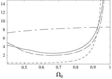
FIG. 5.: This figure shows the bounds (52)–(55) as a function of $\Omega_{0}$. The dotted-dashed line corresponds to the actual constraint on the scalar component, $(H_{T}/\sqrt{\epsilon}M_{\rm Pl})\times 10^{5}$ for a scale invariant scalar spectrum. The rest are upper bounds, on $H_{F}/H_{T}$ (solid line), on $A_{C}\times 10^{4}$ (dashed line), and on $\epsilon/z$ (dotted line). As can be seen, for $\Omega_{0}\simeq 1$, the upper bounds are not very restrictive.

As mentioned in Section 2, single-field models of open inflation [8] require some fine-tuning in order to have a large mass for successful tunneling and a small mass for slow-roll inside the bubble [9]. Even if such a model can be constructed from particle physics, it still needs to satisfy the constraints coming from observations of the CMB anisotropies. In the thin wall regime, these models lack both supercurvature modes  [12] and semi-classical anisotropies, by construction. However, in some cases, they produce too large tensor anisotropies at low multipoles [28], where they are dominated by the bubble-wall fluctuations.

Let us analyse a typical example, which is a variant of the new inflation type [8]. The potential is a quartic double well, to which a double barrier has been added near the origin. Tunneling occurs from a symmetric phase at $\sigma=0$ to a value $\sigma_{b}$ from which the field slowly rolls down the potential towards the symmetry breaking phase at $\sigma=v\sim M_{\rm GUT}\sim 10^{15}$ GeV. The fact that we have a finite number of e-folds, $N_{e}=60$, requires $\sigma_{b}\sim v\,\exp(-\alpha N_{e})\ll v$, where $\alpha\simeq m_{T}^{2}/3H_{T}^{2}$. The rate of expansion in the true vacuum is of the order of that in the false vacuum, $H_{T}\simeq(8\pi V(0)/3M_{\rm Pl}^{2})^{1/2}\sim 3\times 10^{-6}M_{\rm Pl}$, which implies $\epsilon\sim 10^{-3}$, for agreement with CMB anisotropies. Choosing a typical mass in the false vacuum to be $M\sim M_{\rm GUT}$, we find

$$b_{\rm single}\simeq\Big{(}{\sigma_{b}\over M_{\rm Pl}}\Big{)}^{2}{M\over H_{T}}\sim 5\times 10^{-9}\,,$$ (64)

which gives $z\sim 2b\sim 10^{-8}$, an extremely small number that makes it impossible to satisfy the bubble-wall constraint, $\epsilon<z$, see Eq. (54). In other words, the simplest single-field models of open inflation [8] are not only fine-tuned but actually produce too large gravitational-wave anisotropies in the CMB on large scales to be consistent with observations. The reason for that is that in a new inflation type potential, slow roll has to begin very close to $\sigma=0$ in order to have sufficient inflation. However, this does not leave much room for a sufficiently thick barrier.

Linde has recently proposed a new single-field open inflation model [55] in which the two different mass scales needed for tunneling and for slow-roll can coexist. This is basically a quadratic potential, where a barrier is appended at $\phi\sim 3M_{\rm Pl}$. Although the model is somewhat ad hoc from the point of view of particle physics, there is in principle the possibility of making the barrier sufficiently thick, so that the bubble wall fluctuations will not be important. This model has specific signatures of its own [55, 56].

B Coupled and uncoupled two-field models

In this section we shall consider a class of two-field models [9] with a potential of the form

$$V(\sigma,\phi)=V_{0}(\sigma)+{1\over 2}m^{2}\phi^{2}+{1\over 2}g^{2}\sigma^{2}\phi^{2}.$$ (65)

Here $V_{0}$ is a non-degenerate double well potential, with a false vacuum at $\sigma=0$ and a true vacuum at $\sigma=v$. When $\sigma$ is in the false vacuum, $V_{0}$ dominates the energy density and we have an initial de Sitter phase with expansion rate given by $H_{F}^{2}\approx 8\pi V_{0}(0)/3M_{\rm Pl}^{2}$. Once a bubble of true vacuum $\sigma=v$ forms, the energy density of the slow-roll field $\phi$ may drive a second period of inflation. However, as pointed out in Ref. [9], the simplest two-field model of open inflation, given by (65) with $g=0$ and $m\neq 0$, i.e the uncoupled two-field model, is actually a quasi-open one; this is so because equal-time hypersurfaces, defined by the $\sigma$ field after nucleation, are not synchronized with equal-density hypersurfaces, determined by the slow-roll of the $\phi$ field during inflation inside the bubble. In order to suppress this effect it was argued [9] that a large rate of expansion in the false vacuum with respect to the true vacuum, $H_{F}\gg H_{T}$, could prevent the $\phi$ field from rolling outside the bubble and distorting the equal-density hypersurfaces inside it. However, this would induce [27] a large supercurvature mode anisotropy in the CMB, which would be incompatible with observations. A careful analysis [20, 21] shows that indeed the effect is important at low multipoles. In this model, $m_{F}=m_{T}=m$, the supercurvature eigenvalue $\gamma=2m_{F}^{2}/3H_{F}^{2}$, and in order to satisfy (55) it requires

$${H_{F}\over H_{T}}>\Big{(}{D_{l}^{C}/A_{C}^{2}\over D_{l}^{S}/A_{S}^{2}}\Big{)}^{1/4}{1\over\sqrt{A_{S}}}\approx 60\,,$$ (66)

which is incompatible with the supercurvature constraint

$${H_{F}\over H_{T}}<\Big{(}{D_{l}^{S}/A_{S}^{2}\over D_{l}^{SC}/A_{SC}^{2}}\Big{)}^{1/2}{1\over\sqrt{2}}\approx 3\,.$$ (67)

On the other hand, for values of $\Omega_{0}\gtrsim 0.9$, combining the bounds (61) and (63) we find that

$$137\,(1-\Omega_{0})^{1/2}\lesssim\frac{H_{F}}{H_{T}}\lesssim 0.6\,(1-\Omega_{0})^{-1},$$ (68)

which cannot be satisfied unless $\Omega_{0}\gtrsim 0.97$, see Fig. 6. Therefore, this model seems to be ruled out for $\Omega_{0}\lesssim 0.97$.

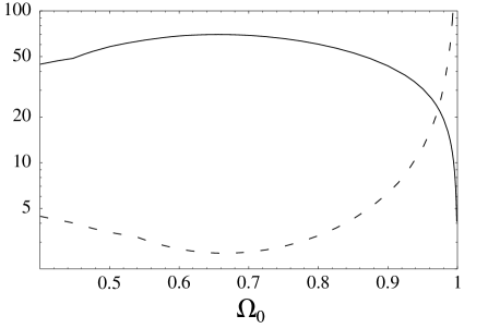
FIG. 6.: Constraints on $H_{F}/H_{T}$ due to supercurvature and semiclassical fluctuations in the uncoupled open inflation model. The region above the dashed line (due to supercurvature fluctuations) and below the solid line (due to semiclassical fluctuations) is excluded by observations. The region allowed by observations (the small corner to the right of the picture) leaves only values of $\Omega_{0}$ that are very close to 1.

In order to construct a truly open model, Linde and Mezhlumian suggested taking $m=0$ and $g\neq 0$, i.e. the coupled two-field model [9]. In this way, the mass of the slow-roll field vanishes in the false vacuum, and it would appear that the problem of classical evolution outside the bubble is circumvented. However, as we showed in Ref. [21], this is not exactly so, and actually the whole class of models (65) leads to quasi-open Universes, which are constrained by CMB observations. Let us work out those constraints in detail here. We will assume a tunneling potential like [9]

$$V_{0}(\sigma)=V_{0}+{1\over 2}M^{2}\sigma^{2}-\alpha M\sigma^{3}+{1\over 4}\lambda\sigma^{4}\,.$$ (69)

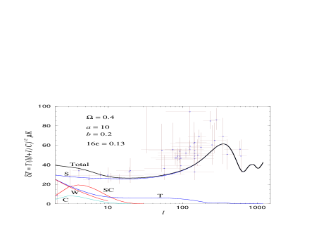
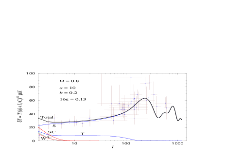
FIG. 7.: The complete angular power spectrum of temperature anisotropies for the coupled two-field model with $\Omega_{0}=0.4$ (higher plot) and $\Omega_{0}=0.8$ (lower plot), for $(a=10,b=0.2)$. We have chosen as cosmological parameters $h=0.70,\ \Omega_{B}=0.05,\ \Omega_{\Lambda}=0,\ N_{\nu}=3.04$. We show the individual contributions from the scalar (S), tensor (T), supercurvature (SC), semi-classical (C) and bubble-wall (W) modes. Note that the bubble-wall mode is responsible for the large growth of the tensor contribution at low multipoles. Only the scalar modes remain beyond about $l=50$, where they grow towards the first acoustic peak. For comparison, we have superimposed the available CMB anisotropy data, as compiled by Tegmark [58]

For simplicity we will take $\alpha=\sqrt{\lambda}$. Then the field can tunnel for $\phi<\phi_{c}=M/g$, when the minimum of the potential at $\sigma\neq 0$ is deeper than the minimum at $\sigma=0$. The constant $V_{0}\simeq 2.77M^{4}/\lambda$ has been added to ensure that the absolute minimum, at $\phi=0$ and $\sigma_{0}\simeq 1.3\,\sigma_{c}$, has vanishing cosmological constant. Here $\sigma_{c}$ is the minimum for $\phi=\phi_{c}$. After tunneling, the field $\phi$ moves along an effective potential $V(\phi)=m_{T}^{2}\phi^{2}/2$, where the effective mass varies only slightly from tunneling to the end of inflation, $m_{T}\simeq 1.3\,g\sigma_{c}$. This potential drives a period of chaotic inflation with slow-roll parameters $\epsilon=\eta=1/2N_{e}\simeq 1/120$. Substituting into (52) we find $H_{T}=6.3\,m_{T}\simeq 8\times 10^{-6}M_{\rm Pl}$, and therefore $g\sigma_{c}=10^{-6}M_{\rm Pl}$. The rate of expansion in the false vacuum is determined from $H_{F}^{2}/H_{T}^{2}=1+4ab$, where $b=(4\pi\sqrt{2}/3\lambda)M^{3}/H_{T}M_{\rm Pl}^{2}$, which gives

$$M={(1+4ab)^{1/2}\over 4b}\,H_{F}\geq\sqrt{2}H_{F}\,,$$ (70)

the last condition arising from preventing the formation of the bubble through the Hawking–Moss instanton, see Ref. [9]. Furthermore, taking $m_{F}=0$ in the equation (24) for the eigenvalue $\gamma$ gives

$$A_{C}={3\over 16}{H_{F}^{2}\over H_{T}^{2}}(R_{0}H_{T})^{4}={3(1+4ab)\over 16[1+(a+b)^{2}]^{2}}<3\times 10^{-4}\,.$$ (71)

From the supercurvature mode condition (53), $(1+4ab)^{1/2}<3$, together with (70) we find the constraint $b<1/2$. From Eq. (71), we realize that having nearly degenerate vacua, $a\ll 1$, is not compatible with observations. Satisfying (71) would require $b\ll 1$ and $a\gg 1$. However, for these values of the parameters we expect large tensor contributions, see Refs. [28, 57] (unless of course $\Omega_{0}$ is sufficiently close to one.) So there should be a compromise between the different mode contributions.

We have shown in Fig. 7 the complete temperature power spectrum for a coupled two-field model having $a=10$ and $b=0.2$, for $\Omega_{0}=0.4$ and $\Omega_{0}=0.8$, which are consistent with observations. It has contributions from all the modes: scalar, tensor, supercurvature, semi-classical and bubble-wall. Note, however, that the bubble-wall mode is in fact included in the sharp growth of the tensor contribution at small multipole number, as emphasized in Ref. [19] and shown explicitly in Fig. 7, and should not be counted twice. Although it is in principle possible to construct a model consistent with observations, the parameters of such a model are not very natural. In order to suppress the associated semi-classical anisotropy we had to choose special values of the parameters. As can be seen from Fig. 7, there still exists a range of parameters for which all contributions to the CMB anisotropies are compatible with present observations. However, future observations by MAP and Planck surveyor will help constrain or even rule out such models.

C Supernatural open inflation

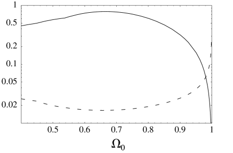
FIG. 8.: Constraints on $R_{0}H_{T}$ due to supercurvature and semiclassical fluctuations in the supernatural open inflation model. The region below the solid line (due to supercurvature fluctuations) and above the dashed line (due to semiclassical fluctuations) is excluded by observations. The region allowed by observations (the small corner to the right of the picture) leaves only values of $\Omega_{0}$ that are very close to 1.

This model consists of a complex scalar field with a slightly tilted Mexican hat potential, where the radial component of the field does the tunneling and the pseudo-Goldstone mode does the slow-roll. This model was called “supernatural” inflation in Ref. [9], because the hierarchy between tunneling and slow-roll mass scales is protected by an approximate global $U(1)$ symmetry. Expanding the field in the form $\Phi=(\sigma/\sqrt{2})\exp(i\phi/v)$, where $v$ is the expectation value of $\sigma$ in the broken phase, we consider a potential of the form $V=V_{0}(\sigma)+V_{1}(\sigma,\phi)$, where $V_{0}$ is $U(1)$-invariant and $V_{1}$ is a small perturbation that breaks this invariance. It is assumed that $V$ has a local minimum at $\Phi=0$, which makes the symmetric phase metastable. We shall consider a tilt in the potential of the form $V_{1}=\Lambda^{4}(\sigma)G(\phi)$, where $\Lambda$ is a slowly varying function of $\sigma$ that vanishes at $\sigma=0$. For definiteness we can take $G=(1-\cos\phi/v)$. The idea is that $\sigma$ tunnels from the symmetric phase $\sigma=0$ to the broken phase $\sigma_{0}=v$, landing at a certain value of $\phi$ away from the minimum of the tilted bottom. Once in the broken phase, the potential $V_{1}$ cannot be neglected, and the field $\phi$ slowly rolls down to its minimum, driving a second period of inflation inside the bubble. Depending on the value of $\phi$ on which we end after tunneling, the number of $e$-foldings of inflation will be different.

As in the two field model, the soft mode which corresponds to a change in the value of $\phi$ after tunneling manifests itself as a supercurvature mode which leads to quasiopen inflating islands. For the generic potential

$$V_{1}(\phi)=\Lambda^{4}\Big{(}1-\cos{\phi\over v}\Big{)}\,,$$ (72)

we find the slow-roll parameters

$$\epsilon = {1\over 2\kappa^{2}v^{2}}\cot^{2}{\phi\over 2v}\ll 1\,,$$ (73)

$$\eta = \epsilon-{1\over 2\kappa^{2}v^{2}}\,.$$ (74)

From the constraint on the spectral tilt, $n_{S}-1=-4\epsilon-1/\kappa^{2}v^{2}>-0.2$, we find that, necessarily, $\kappa^{2}v^{2}>5$, which means that the vev of $\sigma$ is $v\simeq M_{\rm Pl}$. We are again in a situation similar to the single-field models, where we need some extreme fine-tuning to prevent the Hawking–Moss instanton from forming the bubble, see Ref. [9]. Indeed, for a generic tunneling potential like (69) we have $V_{0}\simeq M^{2}\sigma_{0}^{2}/2$ and thus $H_{F}\simeq 2M\,\sigma_{0}/M_{\rm Pl}\geq M$. Under this condition the tunneling does not occur along the Coleman–DeLuccia instanton, which is necessary for the formation of an open Universe inside the bubble. The only way to prevent this is by artificially bending the potential so that it has a large mass at the false vacuum. In Ref. [9] a way was proposed to lower the minimum at the center of the Mexican hat, using radiative corrections from a coupling of the $U(1)$ field $\Phi$ to another scalar $\chi$. For certain values of the coupling constant, $g^{4}=32\pi\lambda$, it is possible to make the two minima, at $\sigma=0$ and $\sigma_{0}$, exactly degenerate. The tunneling potential is then

$$V_{0}(\sigma)={\lambda\over 2}(\sigma_{0}^{2}-\sigma^{2})\sigma^{2}+\lambda\sigma^{4}\,\ln{\sigma\over\sigma_{0}}\,,$$ (75)

where $\sigma_{0}=M/\sqrt{\lambda}\simeq M_{\rm Pl}$. The associated tunneling parameters become $a=0$ and $b=(\sigma_{0}/M_{\rm Pl})^{2}M/H_{T}\simeq M/H_{T}$, which can be large. As emphasized in Ref. [21], there is a supercurvature mode in this model, associated with the massless Goldstone mode, which induces both supercurvature and semi-classical perturbations. Because of the different normalization of the supercurvature mode in supernatural inflation, $H_{F}\to 2R_{0}^{-1}$, the supercurvature constraint (53) should read, in this case:

$$R_{0}H_{T}>2\sqrt{2}\,\Big{(}{D_{l}^{SC}/A_{SC}^{2}\over D_{l}^{S}/A_{S}^{2}}\Big{)}^{1/2}\approx 0.7\,,$$ (76)

which is not trivially satisfied, even for degenerate minima. On the other hand, the eigenvalue $\gamma=R_{0}^{2}m_{T}^{2}/2$ for the Goldstone mode [21] induces a large semi-classical perturbation (55) unless

$$R_{0}H_{T}<\sqrt{4A_{S}\over 3}\,\Big{(}{D_{l}^{S}/A_{S}^{2}\over D_{l}^{C}/A_{C}^{2}}\Big{)}^{1/4}\approx 0.02\,.$$ (77)

It is clear that these two constraints cannot be accommodated simultaneously. For values of $\Omega_{0}>0.9$, the bounds give

$$3\,(1-\Omega_{0})\lesssim R_{0}H_{T}\lesssim 0.008\,(1-\Omega_{0})^{-1/2},$$ (78)

which cannot be satisfied unless $\Omega_{0}\gtrsim 0.98$, see Fig. 8. Therefore, the model is incompatible with observations for $\Omega_{0}\lesssim 0.98$.

D Induced gravity open inflation

This model was proposed in Ref. [24] as a way of avoiding the problems of classical motion outside the bubble. The inflaton field is trapped in the false vacuum due to its non-minimal coupling to gravity, with coupling $\xi$. When the tunneling occurs it is left free to slide down its symmetry breaking potential $V(\varphi)=\lambda(\varphi^{2}-\nu^{2})^{2}/8$. The expectation value of the inflaton at the global minimum gives the Planck mass today: $M_{\rm Pl}^{2}=8\pi\xi\nu^{2}$. The model is parametrized by $\alpha=8U_{F}/\lambda\nu^{4}$, which determines the value of the stable fixed point in the false vacuum, $\varphi_{\rm st}^{2}=\nu^{2}(1+\alpha)$, as well as the difference in the rates of expansion in the false and true vacua, $H_{F}^{2}=H_{T}^{2}\,(1+\alpha)/\alpha$, and the slow-roll parameters, $\epsilon=8\xi/(1+6\xi)\alpha^{2}$, $\eta=8\xi\,(1-\alpha)/(1+6\xi)\alpha^{2}$, see Ref. [25].

We will assume, for the $\sigma$ field, a tunneling potential of the type

$$U(\sigma)={1\over 4}\lambda^{\prime}\sigma^{2}(\sigma-\sigma_{0})^{2}+\mu U_{0}\Big{[}1-\Big{(}{\sigma\over\sigma_{0}}\Big{)}^{4}\Big{]}\,,$$ (79)

where $\sigma_{0}=M\sqrt{2/\lambda^{\prime}}$, $U_{0}=M^{4}/4\lambda^{\prime}$ and $\mu\ll 1$ for the thin-wall approximation to be valid. This potential gives a tunneling parameter $b=(2\pi/3\lambda^{\prime})M^{3}/H_{T}M_{\rm Pl}^{2}$, which determines the relation between the mass of the $\sigma$ field in the false vacuum and the rate of expansion there, $M=H_{F}\,(1+1/\alpha)^{1/2}/\mu b$. Thanks to $\mu\ll 1$, we can have $M\gg H_{F}$ for values of $b\geq 1$, which induces gravitational-wave anisotropies that are well under control.

Furthermore, the induced gravity model seems to be truly open, since the inflaton field $\varphi$ is static in the false vacuum and there is thus no supercurvature mode associated with classical motion outside the bubble, see Ref. [21]. Therefore the constraint (55) does not apply, and there exists for this model a range of parameters for which all contributions to the CMB anisotropies are compatible with observations, see Ref. [28]. However, the instanton may not take you to $\varphi_{\rm st}$ in the true vacuum, but to a different value, closer to the minimum of the potential, $\varphi=v$. In that case, the number of $e$-folds is smaller than expected, and so is the value of $\Omega_{0}$. Such effects should be taken into account for the determination of the model parameters.

E Open hybrid inflation

This model was proposed recently [26], in an attempt to produce a significantly tilted scalar spectrum in the context of open inflation, in order to be in agreement with large scale structure [59]. It is based on the hybrid inflation scenario [60, 61], which has recently received some attention from the point of view of particle physics [62, 63, 64, 65, 66], together with a tunneling field that sets the initial conditions inside the bubble.

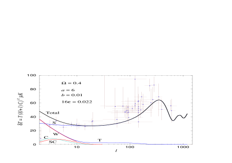
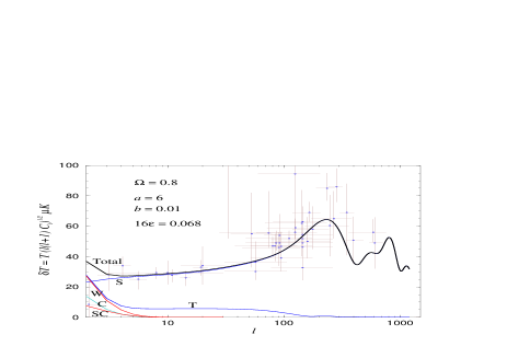
FIG. 9.: The complete angular power spectrum of temperature anisotropies for the open hybrid model with $\Omega_{0}=0.4$ (higher plot) and $\Omega_{0}=0.8$ (lower plot), for $(a=6,b=0.01)$. The cosmological parameters are the same as in Fig. 7. We show the individual contributions from the scalar, tensor, supercurvature, semi-classical and bubble-wall modes. Note that the bubble-wall mode is responsible for the large growth of the tensor contribution at low multipoles. Only the scalar modes remain beyond about $l=50$, where they grow towards the first acoustic peak.

In this model there are three fields: the tunneling field $\sigma$, the inflaton field $\phi$ and the triggering field $\psi$. The tunneling occurs as in the coupled model of Section VI B with potential

$$U(\sigma,\phi)=V_{0}+{\lambda\over 4}\sigma^{2}(\sigma-\sigma_{c})^{2}+{1\over 2}g^{2}(\phi^{2}-\phi_{c}^{2})\sigma^{2}+U_{0}\,,$$ (80)

where $\sigma_{c}=2M/\sqrt{\lambda}$,  $\phi_{c}=M/g$,  $V_{0}\simeq 2.77M^{4}/\lambda$, to ensure that at the global minimum we have vanishing cosmological constant, and $U_{0}$ is the vacuum energy density associated with the triggering field. We satisfy $V_{0}\ll U_{0}$. If the $\sigma$ field tunnels when $\phi=\phi_{T}=3\phi_{c}/4$, then $\Delta U=U_{F}-U_{T}\simeq V_{0}/2\simeq m_{T}^{2}\phi_{c}^{2}/4$. After that, the inflaton field will slow-roll down the effective potential $U=U_{0}+m_{T}^{2}\phi^{2}/2\simeq U_{0}$ driving hybrid inflation, until the coupling to $\psi$ triggers its end. The model is parametrized by $\alpha=m_{T}^{2}/H^{2}_{T}$, see Refs. [26, 28, 57], in terms of which the spectral tilts can be written as $n_{S}-1=2\alpha/3-6\epsilon$ and $n_{T}=-2\epsilon$. At tunneling we can write $V_{0}\simeq m_{T}^{2}\phi_{c}^{2}/2=8m_{T}^{2}\phi_{T}^{2}/9$, so that the slow-roll parameter $\epsilon=(\alpha/3)9V_{0}/16U_{T}=3\alpha ab/2$, where $4ab=\Delta U/U_{T}\simeq V_{0}/2U_{T}$, see (2), and thus

$$n_{S}=1+{2\alpha\over 3}\,\Big{(}1-{27ab\over 2}\Big{)}.$$ (81)

In order for open hybrid models to have a large tilt, we require both a large value of $\alpha$ and a small value of $ab$. As we will show, this will be impossible given the constraints (52–55) from the CMB. For that purpose, we should first compute the tunneling parameters $a=M/2H_{T}$ and $b=(4\pi\sqrt{2}/3\lambda)M^{3}/H_{T}M_{\rm Pl}^{2}\simeq(V_{0}/4U_{T})\,H_{T}/M=2ab\,H_{T}/M$. Since both $H_{T}<M$ and $V_{0}\ll U_{T}$, we expect $a>1$ and $b\ll 1$, which will induce large tensor anisotropies at low multipoles. This is a generic feature of open hybrid models. In order to satisfy the CMB constraints we require

$$H_{F}^{2}/H_{T}^{2} = 1+4ab\lesssim 10\,,$$ (82)

$$\epsilon = {3\alpha ab\over 2}\lesssim{2b\,(0.6)\over[1+(a+b)^{2}]^{1/2}}\,,$$ (83)

$$A_{C} = {3(1+4ab)\over 16[1+(a+b)^{2}]^{2}}\lesssim 3\times 10^{-4}\,,$$ (84)

$$M = {2a\over(1+4ab)^{1/2}}H_{F}>H_{F}\,.$$ (85)

Note that $M_{F}^{2}\approx 2M^{2}>2H_{F}^{2}$. Since $a>1$ requires $b<V_{0}/8U_{T}\ll 1$, we can use the third constraint to get the bound $a>5$, which then imposes (through the second constraint) that $\alpha\lesssim 0.8/a(1+a^{2})^{1/2}\simeq 1/a^{2}<1/30$. This means that the scalar tilt (81) cannot be significantly larger than 1, as was the aim of Ref. [26].

We have plotted in Fig. 9 the complete angular power spectrum of temperature anisotropies for the open hybrid model, in the case $\Omega_{0}=0.4$ and $\Omega_{0}=0.8$, for $(a=6,b=0.01)$. In order to prevent the tensor contribution from exceeding the cosmic variance, we had to reduce the scalar spectral tilt to $n=1.002$, which is essentially scale invariant and may not be sufficient to allow consistency with the large-scale structure [59]. Furthermore, as we decrease in $\Omega_{0}$ it will be necessary for scalar spectra to be closer and closer to scale invariance, in order to reduce the tensor contribution. In any case, there exists for this model a range of parameters for which all contributions to the CMB anisotropies, see e.g. Fig. 9, are compatible with observations, even for low values of $\Omega_{0}$. Of course, as we approach $\Omega_{0}\approx 1$, it is much more likely to accommodate the bounds.

VII Probability distribution for $\Omega_{0}$

As mentioned in Section IV, stronger constraints on two field models arise if we take into account the probability distribution for $\Omega_{0}$, which was considered in Ref. [22]. Inside a given bubble, there will be observers which will measure all possible values of $\Omega_{0}$, and the probability for a given value of $\Omega_{0}$ is taken to be proportional to the number of collapsed objects of galactic size that would form in all regions with that value of $\Omega_{0}$. This probability is the product of three competing factors. One is the “tunneling” factor, which basically corresponds to Eq. (18) and tends to suppress large values of $\phi_{0}$, favouring low values of $\Omega_{0}$. The other is the “anthropic” factor, related to structure formation. The formation of objects of galactic size is suppressed in a low density universe, and so this factor favours large values of $\phi_{0}$. Finally, there is also a volume factor, taking into account that longer inflation leads to more galaxies, although for model parameters where this factor is dominant, the probability distribution is sharply peaked at $\Omega_{0}=1$.

We should emphasize that we are assuming that the slow-roll field outside the bubble does not affect the geometry of de Sitter space. If, for instance, the Universe outside the bubble is in a process of self-reproduction, the probability distribution for $\Omega_{0}$ inside the bubble may be affected. This issue requires further investigation.

With the above assumptions, it was found that, in terms of the variable

$$x\equiv\left({1-\Omega_{0}\over\Omega_{0}}\right),$$

the logarithmic distribution $W=dP/d\ln x$ is peaked at the value

$$x_{\rm peak}\approx\kappa^{-1}\left({3\over 2}\mu-{5\over 4}\right)^{1/2},$$ (86)

where $\kappa\sim 0.1$ is a parameter related to structure formation, and $\mu$ is given by:

$$\mu={\pi^{2}\over 6}R_{0}^{4}V(\phi_{0})\epsilon={1\over 16A_{S}^{2}[1+\Delta^{2}]^{2}}.$$ (87)

Near the peak value, the probability distribution $W$ is Gaussian, with r.m.s. given by

$$\Delta\ln x\sim(6\mu-5)^{-1/2}$$ (88)

These expressions are valid for $\mu\gtrsim 1$. For smaller values, the peak is at $x=0$, meaning that most observers will see a flat universe. On the other hand, the value of $\mu$ should not be too large, say $\mu\lesssim 3$, otherwise, from (86) and (88), we would have $\ln x_{\rm peak}\gtrsim 3$ and $\Delta\ln x\lesssim 0.3$, so the observed value, $x\sim 1$, would be many standard deviations away from the peak value.

Using $A_{S}\approx 5\times 10^{-5}$, and Eqs. (82)–(83), we have $a\approx(4A_{S}\mu^{1/2})^{-1/2},\ b\lesssim 4.5A_{S}^{1/2}\mu^{1/4}$ and

$$\epsilon\lesssim 10^{-3}\mu^{1/2}.$$ (89)

In the coupled model, $\epsilon\sim 10^{-2}$ and this constraint is not satisfied for $\mu\lesssim 3$. One possibility would be to increase the value of the parameter $\mu$, but then a value of $\Omega_{0}\gtrsim 0.1$ would be extremely unlikely. Thus, the coupled model does not seem to accomodate well an intermediate value of the density parameter $0.1\lesssim\Omega_{0}\lesssim 0.7$, and produce at the same time sufficiently small CMB anisotropies. However, we must recall that for values of $\Omega_{0}$ close to 1, the constraints from supercurvature and bubble wall anisotropies are significantly reduced. The constraints (82-83) can then be substituted by (61-62), and (89) is replaced by

$$\epsilon\lesssim 4\times 10^{-6}(1-\Omega_{0})^{-4}\mu^{1/2}.$$

Thus, for $(1-\Omega_{0})\sim 0.1$, the constraints are satisfied even for $\epsilon\sim 10^{-2}$.

For the sake of illustration, let us take $\mu=1$. Then the probability distribution for $\Omega_{0}$ is peaked in the interesting range: all values $0.1\lesssim\Omega_{0}\lesssim 0.9$ fall within one standard deviation or so from the peak value and are not strongly suppressed. This value of $\mu$ can be obtained by taking $a=50$ and, for instance, $b=0.08$. Such values of $a$ and $b$ would lead to unacceptably large supercurvature and wall fluctuation anisotropies if we take, say $\Omega_{0}\lesssim 0.8$. However, for $\Omega_{0}\gtrsim 0.85$ we find that the anisotropies are below the observational bounds (see Fig. 10). Therefore, the coupled model is in good shape if the measured value of $\Omega_{0}$ turns out to be not too far from 1. This is very simple to understand: in that limit, all the effects of the bubble wall are strongly suppressed.

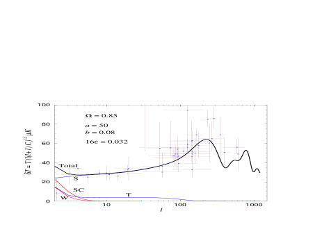
FIG. 10.: The complete angular power spectrum of temperature anisotropies for the coupled model (top panel) and for the open hybrid model (bottom panel) with $\Omega_{0}=0.85$, for $(a=50,b=0.08)$. The cosmological parameters are the same as in Fig. 7.

This should be compared with the situation in Fig. 7. There, the CMB map is acceptable even for $\Omega_{0}=0.4$. However, with $a=10$, we have $\mu\sim 10^{3}$. In this case the peak value is at $\ln x_{\rm peak}\simeq 6$ and the standard deviation is $\Delta\ln x\approx 0.01$. This means that the “measured” value $\Omega_{0}=0.4$ used for that plot is formidably unlikely. For those values of the parameters, most observers within the same bubble would measure much smaller values of the density parameter.

Finally, for the open hybrid model [26], the parameter $\epsilon$ can be made as small as desired, and the condition (89) can be easily satisfied. The reason is that in this model the range of values of the inflaton field are well below Planck scale and the probability distribution (18) easily covers those values within one “standard deviation”.

VIII Conclusions

Single-bubble open inflation is an ingenious way of reconciling an infinite open Universe with the inflationary paradigm. In this scenario, a symmetric bubble nucleates in de Sitter space and its interior undergoes a second stage of slow-roll inflation to almost flatness. At present there is a growing number of experiments studying the CMB temperature anisotropies at fractions of a degree resolution (corresponding to multipole ranges $l=20-500$), and they already put some contraints on the spatial curvature of the universe. However, in the near future, observations of the CMB anisotropies with MAP and Planck will determine whether we live in an open Universe or not with better than 1% accuracy. It is therefore crucial to know whether inflation can be made compatible with such a Universe. Single-bubble open inflation models provide a natural scenario for understanding the large-scale homogeneity and isotropy, but most importantly, they generically predict a nearly scale invariant spectrum of density and gravitational wave perturbations. Future observations of CMB anisotropies and large scale structure power spectra will determine whether these models are still valid descriptions. For that purpose, it is necessary to know the predicted spectrum with great accuracy. In this paper we have explored the CMB anisotropy spectrum for various models of single-bubble open inflation. A host of features at low multipoles due to bubble wall fluctuations, supercurvature modes and quasiopenness place significant constraints on these models.

In particular, we find that the simplest uncoupled two-field model and the “supernatural” model can only accomodate CMB observations provided that $\Omega_{0}\geq 0.98$. Similarly, the simplest single-field models of open inflation, based on a modification of new inflationary potentials with the addition of a barrier near the origin, induce too large tensor anisotropies in the CMB unless the universe is sufficiently flat. Other single field models, where a barrier is suitably appended to a generic slow-roll potential far from the origin may not suffer from this problem [55].

For the coupled two-field model, there is a range of parameters for which all constraints from CMB anisotropies are satisfied even if $\Omega_{0}$ is rather low (say $\Omega_{0}\approx 0.4$). On the other hand, as argued in [22] (see Section VI), stronger constraints arise if we consider the probability distribution for the density parameter for a given set of model parameters, and require that the measured value of $\Omega_{0}$ is not too unlikely in the ensemble of all possible observers inside the bubble. In that case, CMB constraints can still be accomodated provided that $\Omega_{0}\geq 0.85$.

Finally, we have considered the open hybrid model, which was introduced in [26] with the motivation of generating a tilted blue spectrum of density perturbations. In this model, all CMB constraints can be accommodated even for low $\Omega_{0}$. Also, model parameters can be chosen so that typical observers will measure the density parameter in the range $0.1\lesssim\Omega_{0}\lesssim 0.9$. In this sense, the open hybrid model fares better than the coupled two-field model. This is perhaps not too surprising, since this model involves three fields and hence has more free parameters. Even so, it turns out that for the parameter range where the CMB anisotropies are compatible with observations at low multipoles, the tilt of the scalar spectrum is negligible.

In conclusion, we find that existing models of open inflation are strongly constrained by present CMB data. However, there is still for all of them a range of parameters where they would be compatible with observations.

Hawking and Turok [67] have recently proposed that it is possible to create an open universe from nothing in a model without a false vacuum. The instanton describing this process is singular, and therefore its validity has been subject to question [68]. Nevertheless, it has also been pointed out that the quantization of linearized perturbations in the singular background is reasonably well posed [69]. Provided that one can make sense of the instanton by appealing to an underlying theory where the singularity is smoothed out, it seems that the details of that theory need not be known in order to calculate the spectrum of cosmological perturbations. This spectrum can be quite different from that of the one-bubble universe case at large scales (see e.g. [23], where an analytically solvable model was considered), and it deserves further investigation.

A

The open universe scalar harmonics for the subcurvature modes can be written as $Q_{qlm}=\Pi_{ql}(r)\,Y_{lm}(\theta,\phi)$, where [70]

$$\Pi_{ql}(r)=\sqrt{\frac{\Gamma(iq+l+1)\Gamma(-iq+l+1)}{\Gamma(iq)\Gamma(-iq)}}{P_{iq-1/2}^{-l-1/2}(\cosh r)\over\sqrt{\sinh r}}\,.$$ (A1)

Here $Y_{lm}(\theta,\phi)$ are the usual spherical harmonics.

The open universe scalar harmonics for the supercurvature modes ($q^{2}=-\Lambda^{2}$) can be written as ${\cal Y}_{qlm}=\bar{\Pi}_{\Lambda,l}(r)\,Y_{lm}(\theta,\phi)$, where [14]

$$\bar{\Pi}_{\Lambda,l}(r)=\sqrt{{\Gamma(l+1+\Lambda)\Gamma(l+1-\Lambda)\over 2}}{P_{\Lambda-1/2}^{-l-1/2}(\cosh r)\over\sqrt{\sinh r}}\,.$$ (A2)

The various multipoles $l\geq\Lambda$ can be obtained from

$${P_{\Lambda-1/2}^{1/2}(\cosh r)\over\sqrt{\sinh r}} = \sqrt{2\over\pi}\,{\cosh\Lambda r\over\sinh r}\,,$$ (A3)

$${P_{\Lambda-1/2}^{-1/2}(\cosh r)\over\sqrt{\sinh r}} = \sqrt{2\over\pi}\,{\sinh\Lambda r\over\Lambda\sinh r}\,,$$ (A4)

with the recurrence relation

$$(\Lambda^{2}-l^{2})\,P_{\Lambda-1/2}^{-l-1/2}(\cosh r) =$$ (A5)

$$P_{\Lambda-1/2}^{3/2-l}(\cosh r)-(2l-1)\coth r P_{\Lambda-1/2}^{1/2-l}(\cosh r)\,.$$ (A6)

To define the primordial scalar power spectrum we assume that at the end of inflation the scalar metric perturbation takes the form

$${\cal R} \to \sum_{\Lambda}{\cal R}_{\Lambda}{\cal Y}_{\Lambda,lm}$$ (A7)

$$+ \sum_{\pm lm}\int_{0}^{\infty}dq\,{\cal R}_{\pm}(q)Q_{qlm}$$ (A8)

from where the explicit expressions for the amplitudes $A_{S}^{2}$, $A_{SC}^{2}$ and $A_{W}^{2}$ can be read off. The continuum part of the scalar power spectrum is defined as

$$\langle|{\cal R}(q)|^{2}\rangle=\sum_{\pm}|{\cal R}_{\pm}(q)|^{2},$$ (A9)

see [12] for details.

To describe the open universe gravitational waves we use the following notation. The perturbed metric (if we only consider even gravitational perturbations) can be written as

$$ds^{2}=a^{2}(\eta)\left[-d\eta^{2}+(\gamma_{ij}^{(0)}+2h_{ij})dx^{i}dx^{j}\right]\,.$$ (A10)

The perturbation $h_{ij}$ is then expanded as

$$h_{ij}=\sum_{\pm lm}\int_{0}^{\infty}dq\,h_{\pm qlm}(\eta)Q_{ij}^{qlm}(x^{k})\,,$$ (A11)

where the even harmonics $Q_{ij}^{qlm}(x^{k})=G_{ij}^{ql}(r)Y_{lm}(\theta,\phi)$ are transverse and traceless[70, 18, 28], and the radial component is given by

$$G_{rr}^{ql}(r)=\left[\frac{(l-1)l(l+1)(l+2)}{2q^{2}(1+q^{2})}\right]^{1/2}\frac{\Pi_{ql}(r)}{\sinh^{2}r}\,.$$ (A12)

At the end of inflation, the gravitational perturbation takes the form

$$h_{ij}\to\sum_{\pm lm}\int_{0}^{\infty}dq\,h_{\pm}(q)Q_{ij}^{qlm}(x^{k})\,.$$ (A13)

The powers pectrum is then defined as

$$\langle|h(q)|^{2}\rangle=\sum_{\pm}|h_{\pm}(q)|^{2}\,,$$ (A14)

see [18, 19] for details.

B

As mentioned in Section IV, an observer located at a distance $r\gg 1$ from the center of an inflating island would measure an anisotropy due to the gauge invariant perturbation (23). This is caused by a field perturbation $\delta\phi\approx(\gamma/2)\phi_{0}$, where $\phi_{0}$ is the value of the scalar field at the beginning of inflation at the location where the observer lives. We can compare this with the perturbation caused by the $l>0$ supercurvature modes, which is of order $\delta\phi\sim H_{F}/2\pi$. The “semiclassical” anisotropy would only dominate over the usual supercurvature anisotropies when

$$\gamma\phi_{0}\gtrsim H_{F}.$$ (B1)

However, it turns out that such values of $\phi_{0}$ typically occur only near the centers of inflating islands, as the following argument shows [22]. If $\phi_{c}$ is the value at the center, then

$$\phi_{0}\approx\phi_{c}(1-{\gamma\over 6}r^{2}),\quad r\ll 1$$ (B2)

$$\phi_{0}\approx\phi_{c}(1-{\gamma\over 2}r),\quad 1\ll r\ll\gamma^{-1}$$ (B3)

Defining $\Delta\phi=\phi_{c}-\phi_{0}$, the probability for the observer to be at a distance $r$ away from the center can be obtained by expanding the exponent in (18)

$$P(\phi_{0}+\Delta\phi)\propto\exp\Big{[}{-\phi_{0}^{2}\over 2f^{2}}\Big{(}1+2{\Delta\phi\over\phi_{0}}\Big{)}\Big{]}.$$

Hence, the expected $\Delta\phi$ for an observer at $\phi_{0}$ is of order $\Delta\phi\lesssim f^{2}/\phi_{0}$. Using (B3), we see that for values of the field which satisfy (B1), the expected distance to the center of the island is of order

$$r\sim{f^{2}\over\gamma\phi^{2}_{0}}\sim{H_{F}^{2}\over\gamma^{2}\phi^{2}_{0}}\lesssim 1.$$

Therefore, one is led to the conclusion that field values for which the semiclassical anisotropy would be large, satisfying (B1), occur typically near the center of the islands, $r\ll 1$, where the anisotropy is actually not seen!

The same conclusion can be reached from first principles. All the necessary information is contained in the quantum state, a wave functional depending on the amplitudes of the different field multipoles. Expanding the field as $\phi(r,\theta,\varphi)=\sum c_{qlm}Z_{qlm}(x^{i})$, the square of the wave functional will give the probability distribution $P[\phi]=\Pi_{i}P_{i}[c_{i}]$ for the coefficients $c_{i}$, where $i=(q,l,m)$ is a collective index. $P$ factorizes into independent $P_{i}$’s (which are just Gaussian distributions for each $c_{i}$), because we are quantizing linearized perturbations which are decoupled from each other. The quantum state we are using is homogeneous, and we can take any point on the hyperboloid as the origin of coordinates. Let us then take our observer to be at $r=0$, and let us concentrate on the supercurvature sector $q^{2}=-1$. All modes with $l>0$ vanish at the origin. Therefore, the value of the field at $r=0$ only depends on the coefficient $c_{q^{2}=-1,0,0}$ in our universe. The $l=0$ mode is spherically symmetric and hence does not contribute to anisotropies. The anisotropies measured by this observer will only depend on the amplitudes taken by the $c_{i}$ with $l>0$, whose r.m.s. is of order $H_{F}$. From this point of view, it is clear that typical observers will effectively not see the semiclassical anisotropy discussed in Section IV.

However, as discussed above, the “weak” assumption that our value of $\phi_{0}$ is not too special, in the sense that it will occur typically at large distances from the center of the island, implies that $\gamma\phi_{0}\lesssim H_{F}$. In other words, we must impose that the anisotropy induced by the perturbation (23) should always be subdominant with respect to the usual supercurvature anisotropy.

REFERENCES

- [1] See, for instance, S. Perlmutter, 19th Texas Symposium, Paris, December 1998.
- [2] See, for instance, G. Efstathiou, 19th Texas Symposium, Paris, December 1998.
- [3] P.J.E. Peebles, Principles of Physical Cosmology (Princeton University Press, 1993).
- [4] J. Silk and M.S. Turner, Phys. Rev. D 35, 419 (1987); M. S. Turner, ibid. 44, 3737 (1991); A. Kashlinsky, I. Tkachev and J. Frieman, Phys. Rev. Lett. 73, 1582 (1994).
- [5] L.P. Grishchuk and Ya.B. Zel’dovich, Astron. Zh. 55, 209 (1978) [Sov. Astron. 22, 125 (1978)]; J. García-Bellido, A. R. Liddle, D. H. Lyth and D. Wands, Phys. Rev. D 52, 6750 (1995).
- [6] J.R. Gott III, Nature 295, 304 (1982); J.R. Gott III and T.S. Statler, Phys. Lett. 136B, 157 (1984).
- [7] B. Ratra and P.J.E. Peebles, Astrophys.J.432, L5 (1994); Phys. Rev. D 52, 1837 (1995); M. Kamionkowski, B. Ratra, D. Spergel and N. Sugiyama, Astrophys. J. 434, L57 (1994).
- [8] M. Bucher, A.S. Goldhaber and N. Turok, Phys. Rev. D 52, 3314 (1995); K. Yamamoto, M. Sasaki and T. Tanaka, Astrophys. J. 455, 412 (1995).
- [9] A. D. Linde, Phys. Lett. B 351, 99 (1995); A. D. Linde and A. Mezhlumian, Phys. Rev. D 52, 6789 (1995).
- [10] D. H. Lyth and A. Woszczyna, Phys. Rev. D 52, 3338 (1995).
- [11] M. Sasaki, T. Tanaka and K. Yamamoto, Phys. Rev. D 51, 2979 (1995); M. Bucher and N. Turok, Phys. Rev. D 52, 5538 (1995).
- [12] K. Yamamoto, M. Sasaki and T. Tanaka, Phys. Rev. D 54, 5031 (1996).
- [13] T. Hamazaki, M. Sasaki, T. Tanaka and K. Yamamoto, Phys. Rev. D 53, 2045 (1996).
- [14] J. García-Bellido, Phys. Rev. D 54, 2473 (1996).
- [15] J. Garriga, Phys. Rev. D 54, 4764 (1996).
- [16] J. D. Cohn, Phys. Rev. D 54, 7215 (1996).
- [17] J. García-Bellido, A. R. Liddle, D. H. Lyth and D. Wands, Phys. Rev. D 55, 4596 (1997).
- [18] T. Tanaka and M. Sasaki, Prog. Theor. Phys. 97, 243 (1997); M. Bucher and J. D. Cohn, Phys. Rev. D 55, 7461 (1997).
- [19] M. Sasaki, T. Tanaka and Y. Yakushige, Phys. Rev. D 56, 616 (1997); J. Garriga, X. Montes, M. Sasaki and T. Tanaka, Nucl. Phys. B513, 343 (1998).
- [20] J. Garriga and V.F. Mukhanov, Phys. Rev. D 56, 2439 (1997).
- [21] J. García-Bellido, J. Garriga and X. Montes, Phys. Rev. D 57, 4669 (1998).
- [22] J. Garriga, T. Tanaka and A. Vilenkin, astro-ph/9803268 (1998).
- [23] J. Garriga, X. Montes, M. Sasaki, T. Tanaka, astro-ph/9811257 (1998).
- [24] A. Green and A. R. Liddle, Phys. Rev. D 55, 609 (1997).
- [25] J. García-Bellido and A. R. Liddle, Phys. Rev. D 55, 4603 (1997).
- [26] J. García-Bellido and A. Linde, Phys. Lett. B 398, 18 (1997); Phys. Rev. D 55, 7480 (1997).
- [27] M. Sasaki and T. Tanaka, Phys. Rev. D 54, R4705 (1996).
- [28] J. García-Bellido, Phys. Rev. D 56, 3225 (1997).
- [29] S. Coleman and F. De Luccia, Phys. Rev. D 21, 3305 (1980).
- [30] C. L. Bennett et al., Astrophys. J. 464, L1 (1996).
- [31] A. Dekel, astro-ph/9705033 (1997).
- [32] W. Freedman, astro-ph/9706072 (1997).
- [33] C. Lineweaver, D. Barbosa, A. Blanchard and J. Bartlett, Astron. & Astrophys. 322, 365 (1997); Astron. & Astrophys. 329, 799 (1997).
- [34] C. Lineweaver and D. Barbosa, Astrophys. J. 496, 624 (1998).
- [35] S. Parke, Phys. Lett. 121B, 313 (1983).
-
[36]
M. Kamionkowski, D. N. Spergel and N. Sugiyama,
Astrophys. J. 426, L57 (1994);
W. Hu and N. Sugiyama, Phys. Rev. D 51, 2599 (1995). - [37] P. H. Frampton, Y. Jack Ng and R. Rohm, Mod. Phys. Lett. A13 2541 (1998).
- [38] A. R. Liddle and D. H. Lyth, Phys. Rep. 231, 1 (1993).
- [39] B. Allen and R. Caldwell, preprint WISC-MILW-94-TH-21 (unpublished).
- [40] A. A. Starobinsky, Sov. Astron. Lett. 11, 133 (1985) [Pis’ma Astron. Zh. 11, 323 (1985)].
- [41] W. Hu and M. White, Astrophys. J. 486, L1 (1997).
- [42] W. Hu, N. Sugiyama and J. Silk, Nature 386, 37 (1997).
- [43] R. K. Sachs and A. M. Wolfe, Astrophys. J. 147, 73 (1967).
-
[44]
MAP Home Page at
http://map.gsfc.nasa.gov/ (1996). -
[45]
Planck Surveyor Home Page at
http://astro.estec.esa.nl/SA-general/Projects/
Cobras/cobras.html (1996). - [46] G. Jungman, M. Kamionkowski, A. Kosowsky and D. N. Spergel, Phys. Rev. D 54, 1332 (1996).
- [47] M. Zaldarriaga, D. Spergel and U. Seljak, Astrophys. J. 488, 1 (1997).
- [48] J. R. Bond, G. Efstathiou and M. Tegmark, MNRAS 291, L33 (1997).
- [49] L. Knox and M. S. Turner, Phys. Rev. Lett. 73, 3347 (1994).
- [50] U. Seljak and M. Zaldarriaga, Astrophys. J. 469, 437 (1996); D. Spergel and M. Zaldarriaga, Phys. Rev. Lett. 79, 2180 (1997).
- [51] J. R. Bond, in Cosmology and Large Scale Structure, Les Houches Summer School Course LX, ed. R. Schaeffer (Elsevier Science Press, Amsterdam, 1996).
- [52] E. F. Bunn and M. White, Astrophys. J., 480, 6 (1997).
- [53] S. Carroll, W. Press and E. Turner, ARA& A, 30, 499 (1992).
- [54] M. Kamionkowski and A. Loeb, Phys. Rev. D 56, 4511 (1997).
- [55] A.D. Linde gr-qc/9807493 (1998)
- [56] A.D. Linde, M. Sasaki and T. Tanaka, in preparation.
- [57] J. García-Bellido, Single-bubble open inflation: An overview, hep-ph/9803270 (1998).
-
[58]
Max Tegmark web page at
http://www.sns.ias.edu/~max/cmb/experiments.html - [59] M. White and J. Silk, Phys. Rev. Lett. 77, 4704 (1996).
- [60] A.D. Linde, Phys. Lett. B259, 38 (1991); Phys. Rev. D 49, 748 (1994).
- [61] E. Copeland, A. Liddle, D. Lyth, E. Stewart and D. Wands, Phys. Rev. D 49, 6410 (1994).
- [62] L. Randall, M. Soljačić and A. H. Guth, Nucl. Phys. B 472, 377 (1996).
- [63] J. García-Bellido, A. D. Linde and D. Wands, Phys. Rev. D 54, 6040 (1996).
- [64] A.D. Linde and A. Riotto, Phys. Rev. D 56, 1841 (1997).
- [65] C. Panagiotakopoulos, Phys. Rev. D 55, 7335 (1997).
- [66] G. Dvali, G. Lazarides and Q. Shafi, Phys. Lett. B424, 259 (1998).
- [67] S.W. Hawking and N. Turok, Phys. Lett. B425, 25 (1998).
- [68] A. Vilenkin, Phys. Rev. D 57, 7069 (1998); A. Linde, Phys. Rev. D 58, 083514 (1998); W. Unruh, gr-qc/9803050 (1998).
- [69] J. Garriga, hep-th/9803210 (1998).
- [70] E.R. Harrison, Rev. Mod .Phys 39, 862 (1967); L. F. Abbot and R. K. Schaefer, Astrophys. J. 308, 546 (1986)