$\gamma^{*}\gamma^{*}$ total cross-section in the dipole picture of BFKL dynamics

Maarten Boonekamp

Service de Physique des Particules, DAPNIA, CEA-Saclay
91191 Gif sur Yvette Cedex, France

Albert De Roeck

Deutsches Elektronen-Synchrotron, DESY,
Notkestr.85, D-22603 Hamburg, Germany,
and

CERN, CH-1211 Geneve 23, Switzerland

Christophe Royon

Service de Physique des Particules, DAPNIA, CEA-Saclay
91191 Gif sur Yvette Cedex, France

Samuel Wallon

Division de Physique Théorique, Institut de Physique Nucléaire d’Orsay
91406 Orsay, France
and
Laboratoire de Physique Théorique des Particules Elémentaires,
Université P. & M. Curie, 4 Place Jussieu
75252 Paris Cedex 05, France

The total $\gamma^{*}\gamma^{*}$ cross-section is derived in the Leading Order QCD dipole picture of BFKL dynamics, and compared with the one from 2-gluon exchange. The Double Leading Logarithm approximation of the DGLAP cross-section is found to be small in the phase space studied. Cross sections are calculated for realistic data samples at the $e^{+}e^{-}$ collider LEP and a future high energy linear collider. Next to Leading order corrections to the BFKL evolution have been determined phenomenologically, and are found to give very large corrections to the BFKL cross-section, leading to a reduced sensitivity for observing BFKL.

1 Introduction

In this paper we study the possibility to investigate QCD pomeron effects in the high energy limit in virtual photon-photon scattering both at LEP and a future Linear Collider (LC). In the past years, the BFKL pomeron [1] has been studied intensively in the small-$x$ regime at HERA both in the context of proton diffractive and fully inclusive structure functions [2] [3] and of final state particle flow or forward jet production [4]. The coupling to the proton induces a non-perturbative scale in the structure function studies and the studies of final states suffer from non-perturbative hadronisation effects. The use of a purely perturbatively calculable process is much more favourable to establish effects of BFKL dynamics. The cross-section of collisions of two objects with small transverse size is an ideal process where the BFKL approximation is expected to be most reliable. High energy virtual $\gamma^{*}\gamma^{*}$ interactions at $e^{+}e^{-}$ colliders is such a process, and has been proposed in [5, 6, 7] as a laboratory to study BFKL.

In this paper inclusive virtual photon scattering in $e^{+}e^{-}$ collisions at LEP and a future LC is studied. In particular the LC, with an anticipated luminosity three orders of magnitude larger than the one presently at LEP, and its larger centre of mass (CMS) energy of up to 1 TeV, offers an excellent opportunity to test BFKL dynamics.

First we obtain the Leading Order (LO) BFKL cross-section using the QCD dipole picture of BFKL dynamics. The Double Leading Logarithm approximation of the DGLAP cross-section [8] is compared with the BFKL one. The 2-gluon approximation, where only 2 gluons are exchanged in the $\gamma^{*}\gamma^{*}$ interactions will turn out to be the dominant ’background’ in the region of phase space studied in this paper. We will then consider phenomenologically the effects of higher order corrections to the BFKL cross-section, and show that the cross-sections for the 2-gluon and BFKL-NLO evolutions both at the LC and LEP colliders, are different by a factor of two to four.

2 $\gamma^{*}\gamma^{*}$ total cross-section in the dipole picture of BFKL dynamics

2.1 BFKL cross-section

We analyse the $\gamma^{*}\gamma^{*}$ subprocess in the framework of the color dipole model [9, 10, 11, 12].

Figure 1: 2-gluon exchange for the $\gamma^{*}\gamma^{*}$ subprocess in $e^{+}e^{-}\to e^{+}e^{-}+X$ collisions.

As usual, in analogy with Deep Inelastic Scattering (DIS) kinematics, we define the scaling variables which will describe the total cross-section (see Ref. [5], and the scheme in Figure 1 for the definitions of the variables.)

$$y_{1}=\frac{q_{1}k_{2}}{k_{1}k_{2}},\quad y_{2}=\frac{q_{2}k_{1}}{k_{1}k_{2}},$$ (2.1)

and

$$x_{1}=\frac{Q^{2}_{1}}{2q_{1}k_{2}},\quad x_{2}=\frac{Q^{2}_{2}}{2q_{2}k_{1}},$$ (2.2)

the photons having virtualities $Q^{2}_{1}=-q_{1}^{2}$ and $Q^{2}_{2}=-q_{2}^{2}.$ The total energy available in the $s$ channel of the $e^{+}e^{-}$ system is $s=(k_{1}+k_{2})^{2}.$ The energy available for the subprocess $\gamma^{*}\gamma^{*}$ is $\hat{s}=(q_{1}+q_{2})^{2}\simeq sy_{1}y_{2}.$ We consider the domain of large $Q^{2}_{1},\,Q^{2}_{2}$ (in order to be in the perturbative regime) and large $\hat{s}$ with the constraint

$$Q^{2}_{1},\,Q^{2}_{2}\ll\hat{s},$$ (2.3)

in order to exhibit the energy dependence of the BFKL pomeron, which will be described in terms of a dipole cascade. Defining

$$X_{1}=\frac{Q^{2}_{1}}{2q_{1}q_{2}}\simeq\frac{Q^{2}_{1}}{\hat{s}},\quad X_{2}=\frac{Q^{2}_{2}}{2q_{1}q_{2}}\simeq\frac{Q^{2}_{2}}{\hat{s}},$$ (2.4)

the total rapidity of the $\gamma^{*}\gamma^{*}$ subprocess is then given by

$$Y=\ln\frac{1}{\sqrt{X_{1}X_{2}}}\simeq\ln\frac{\hat{s}}{\sqrt{Q^{2}_{1}Q^{2}_{2}}}=\ln\frac{sy_{1}y_{2}}{\sqrt{Q^{2}_{1}Q^{2}_{2}}}.$$ (2.5)

Let us first compute the $\gamma^{*}\gamma^{*}$ total cross-section in the two-gluon exchange approximation. Note that the QED contribution which corresponds to a quark box coupled to four external virtual photons, is sub-leading in the high-energy limit, since $t$-channel exchange of two particles of spin $J$ contributes like $s^{(2J-1)},$ and is thus dominated by gluon contributions.

In the dipole approach, one can view the two virtual photons as two dipoles, which can scatter through the exchange of a pair of soft gluons. This requires the knowledge of the photon wave function. The photon wave function squared $\Phi_{T,L}(\underline{x},z;Q^{2})$ gives the probability distribution of finding a dipole configuration of transverse size $\underline{x},$ $z$ ($(1-z)$) being the light-cone momentum fraction carried by the quark (antiquark). The subscript $T$ ($L$) corresponds to a transversally (longitudinally) polarized photon. Note that we neglect here the effect of quark masses. Heavy quark production will be considered in a future paper.

Explicit expressions for these probability distributions can be found in [13, 12] . We will not use them here.

The cross-section is then obtained by convoluting the two probability distributions with the elementary dipole-dipole cross-section. The latter corresponds to the scattering of two color neutral objects in the eikonal approximation [10, 16]. It reads, if one averages over the angle between the two dipoles ,

$$\bar{\sigma}_{DD}(\underline{x}_{1},\underline{x}_{2})=\alpha_{s}^{2}\int\frac{d^{2}\underline{k}}{(\underline{k}^{2})^{2}}\left(2-e^{\displaystyle i\underline{k}.\underline{x}_{1}}-e^{-\displaystyle i\underline{k}.\underline{x}_{1}}\right)\left(2-e^{\displaystyle i\underline{k}.\underline{x}_{2}}-e^{-\displaystyle i\underline{k}.\underline{x}_{2}}\right)$$ (2.6)

The $\gamma^{*}\gamma^{*}$ cross-section in the two-gluon exchange approximation then reads

$$\sigma_{\gamma^{*}\gamma^{*}}(Q_{1}^{2},Q_{2}^{2};Y)=\int d^{2}\underline{x}_{1}\,dz_{1}\,\int d^{2}\underline{x}_{2}\,dz_{2}\,\Phi(\underline{x}_{1},z_{1};Q_{1}^{2})\,\Phi(\underline{x}_{2},z_{2};Q_{2}^{2})\,\sigma_{DD}(\underline{x}_{1},\underline{x}_{2})\,.$$ (2.7)

Let us consider now the elementary Born cross-section $\hat{\sigma}_{\gamma d}/k^{2}$ of the process

$$d(\mbox{$\underline{x}$})~{}g(k)\rightarrow~{}d(\mbox{$\underline{x}$})$$ (2.8)

for a dipole of transverse size $\underline{x}$ and a soft gluon of virtuality $\underline{k}^{2},$ in light-cone gauge. In the high energy approximation, we only need its expression close to the physical pole $k^{2}=0$. Thus its computation can be performed using the equivalent photon (in this case gluon) approximation of Weizsäcker and Williams [14], setting $k^{2}=0$ in the expression of the classical current of a dipole [2, 15, 16]. This gives, summing over color and polarization of the emitted gluon and averaging over the color of the dipole,

$$\frac{\hat{\sigma}_{gd}}{\mbox{$\underline{k}$}^{2}}=\frac{\alpha_{s}N_{c}}{\pi}\left(2-e^{\displaystyle i\mbox{$\underline{k}$}.\mbox{$\underline{x}$}}-e^{\displaystyle-i\mbox{$\underline{k}$}.\mbox{$\underline{x}$}}\right)\frac{1}{\mbox{$\underline{k}$}^{2}}\,.$$ (2.9)

This squared quantity is related to the elementary dipole-dipole cross-section since it can also be computed using the same equivalent gluon technique.

Indeed, the elementary dipole-dipole cross-section $\bar{\sigma}_{DD}$ reads

$$\bar{\sigma}_{DD}(\underline{x}_{1},\underline{x}_{2})=\frac{(2\pi)^{2}}{4N_{c}^{2}}\int d^{2}\underline{k}\frac{\hat{\sigma}_{gd}}{\mbox{$\underline{k}$}^{2}}\,\frac{\hat{\sigma}_{gd}}{\mbox{$\underline{k}$}^{2}}\,,$$ (2.10)

the factor $\frac{(2\pi)^{2}}{4N_{c}^{2}}$ arising from the normalisation of the $\underline{k}$ integration and from the definition of $\frac{\hat{\sigma}_{gd}}{\mbox{$\underline{k}$}^{2}}$ as an averaged color quantity.

Thus, the $\gamma^{*}\gamma^{*}$ total cross-section in the two-gluon exchange approximation now reads

$$\sigma_{\gamma^{*}\gamma^{*}}(Q_{1}^{2},Q_{2}^{2};Y)=\left(\frac{\pi}{N_{c}^{2}}\right)^{2}\int d^{2}\underline{x}_{1}\,dz_{1}\,\int d^{2}\underline{x}_{2}\,dz_{2}\,\Phi(\underline{x}_{1},z_{1};Q_{1}^{2})\,\Phi(\underline{x}_{2},z_{2};Q_{2}^{2})\,\int d^{2}\underline{k}\frac{\hat{\sigma}_{gd}}{\mbox{$\underline{k}$}^{2}}\,\frac{\hat{\sigma}_{gd}}{\mbox{$\underline{k}$}^{2}}\,.$$ (2.11)

This will give us later the hint to exhibit the relation with the calculation based on Feynman diagrams technique.

Following [17], we define the Mellin-transform of the photon wave function as

$$\tilde{\Phi}(\gamma)=\int\frac{d^{2}\underline{x}}{2\pi}dz\,\Phi_{T,L}(\underline{x},z)(\underline{x}^{2}Q^{2})^{1-\gamma}\,,$$ (2.12)

or equivalently

$$\int dz\,\Phi(\underline{x},z)=\int\frac{d\gamma}{2i\pi}\frac{2}{\underline{x}^{2}}\tilde{\Phi}(\gamma)\,(\underline{x}^{2}Q^{2})^{-1+\gamma}\,.$$ (2.13)

Eq. (2.11) then reads

$$\sigma_{\gamma^{*}\gamma^{*}}(Q_{1}^{2},Q_{2}^{2};Y) = \left(\frac{\pi}{N_{c}^{2}}\right)^{2}\int d^{2}\underline{x}_{1}\,dz_{1}\,\int d^{2}\underline{x}_{2}\,dz_{2}\,\Phi(\underline{x}_{1},z_{1};Q_{1}^{2})\,\Phi(\underline{x}_{2},z_{2};Q_{2}^{2})\,\int d^{2}\underline{k}\frac{\hat{\sigma}_{gd}}{\mbox{$\underline{k}$}^{2}}\,\frac{\hat{\sigma}_{gd}}{\mbox{$\underline{k}$}^{2}}$$ (2.14)

$$= \left(\frac{\pi}{N_{c}^{2}}\right)^{2}\int d^{2}\underline{x}_{1}\,\int d^{2}\underline{x}_{2}\int\frac{d\gamma_{1}}{2i\pi}\int\frac{d\gamma_{2}}{2i\pi}\frac{2}{\underline{x}_{1}^{2}}\tilde{\Phi}(\gamma_{1})\frac{2}{\underline{x}_{2}^{2}}\tilde{\Phi}(\gamma_{2})$$

$$\times\int d^{2}\underline{k}\frac{\hat{\sigma}_{gd}}{\mbox{$\underline{k}$}^{2}}\,(\underline{x}_{1}^{2}Q_{1}^{2})^{-1+\gamma_{1}}(x_{2}^{2}Q_{2}^{2})^{-1+\gamma_{2}}\frac{\hat{\sigma}_{gd}}{\mbox{$\underline{k}$}^{2}}$$

From Eq. (2.9) we have

$$\frac{\pi}{N_{c}}\int\frac{d^{2}\underline{x}}{\underline{x}^{2}}\hat{\sigma}_{gd}=\alpha_{s}\int\frac{d^{2}\underline{x}}{\underline{x}^{2}}\left(2-e^{\displaystyle i\mbox{$\underline{k}$}.\mbox{$\underline{x}$}}-e^{\displaystyle-i\mbox{$\underline{k}$}.\mbox{$\underline{x}$}}\right)=4\pi\alpha_{s}\int\frac{dx}{x}(1-J_{0}(kx))\,.$$ (2.15)

The Mellin transform of this quantity then reads

$$\frac{\pi}{N_{c}}\int\frac{d^{2}\underline{x}}{\underline{x}^{2}}\hat{\sigma}_{gd}(x^{2}Q^{2})^{-1+\gamma}=4\pi\alpha_{s}v(1-\gamma)\left(\frac{k^{2}}{Q^{2}}\right)^{1-\gamma}$$ (2.16)

where (see Ref. [2, 15, 16])

$$v(\gamma)=\frac{2^{-2\gamma-1}}{\gamma}\frac{\Gamma(1-\gamma)}{\Gamma(1+\gamma)}\,.$$ (2.17)

Thus, the $\gamma^{*}\gamma^{*}$ total cross-section now reads

$$\sigma_{\gamma^{*}\gamma^{*}}(Q_{1}^{2},Q_{2}^{2};Y) = 4\int\frac{d\gamma_{1}}{2i\pi}\int\frac{d\gamma_{2}}{2i\pi}\int\frac{d^{2}\underline{k}}{\underline{k}^{4}}4\pi\alpha_{s}v(1-\gamma_{1})4\pi\alpha_{s}v(1-\gamma_{2})\left(\frac{k^{2}}{Q_{1}^{2}}\right)^{1-\gamma_{1}}\left(\frac{k^{2}}{Q_{2}^{2}}\right)^{1-\gamma_{2}}$$ (2.18)

$$\times\,\tilde{\Phi}(\gamma_{1})\tilde{\Phi}(\gamma_{2})=4\pi\int\frac{d\gamma}{2i\pi}4\pi\alpha_{s}\tilde{\Phi}(\gamma)\,v(1-\gamma)4\pi\alpha_{s}\tilde{\Phi}(1-\gamma)\,v(\gamma)\left(\frac{Q_{1}^{2}}{Q_{2}^{2}}\right)^{\gamma}\frac{1}{Q_{1}^{2}}$$

where in the last step the integration with respect to $\underline{k}$ has been performed, leading to $1-\gamma_{2}=\gamma_{1}.$

Let us compare this calculation, based on the dipole approach (light-cone quantization), with the calculation based on Feynman diagram calculation (covariant quantization). In the second approach one has to convolute the two off-shell Born cross-sections $\hat{\sigma}_{\gamma g}/Q_{1}^{2}$ and $\hat{\sigma}_{\gamma g}/Q_{2}^{2}$ of the processes $\gamma(q_{1})~{}g(k)\rightarrow q~{}\bar{q}$ and $\gamma(q_{2})~{}g(k)\rightarrow q~{}\bar{q}.$ Here the gluon is off-shell, quasi transverse, with a virtuality $k^{2}\,\simeq\mbox{$\underline{k}$}^{2}$. The $\gamma^{*}\gamma^{*}$ total cross-section in the two-gluon exchange approximation then reads in this scheme

$$Q_{1}^{2}Q_{2}^{2}\sigma_{\gamma^{*}\gamma^{*}}(Q_{1}^{2},Q_{2}^{2};Y) = \frac{2}{\pi^{4}}\int d^{2}\underline{k}_{1}\int d^{2}\underline{k}_{2}\int^{1}_{0}\frac{dz_{1}}{z_{1}}\int^{1}_{0}\frac{dz_{2}}{z_{2}}\hat{\sigma}_{\gamma g}\left(\frac{X_{1}}{z_{1}},\frac{\underline{k}_{1}^{2}}{Q_{1}^{2}}\right)\,$$ (2.19)

$$\hat{\sigma}_{\gamma g}\left(\frac{-X_{2}}{z_{2}},\frac{\underline{k}_{2}^{2}}{Q_{2}^{2}}\right)\,\delta^{2}(\underline{k}_{1}-\underline{k}_{2})\,,$$

where $z_{1}$ and $z_{2}$ are the light-cone momentum fractions of the exchanged gluon respectively measured with respect to $q_{2}^{-}$ and $q_{1}^{+}$ (compare with DIS where $x_{Bj}$ is the light-cone fraction with respect to the proton momentum). In the light-cone frame, we get

$$q_{1}^{\mu}=(\stackrel{{\scriptstyle+}}{{q_{1}^{+}}},\stackrel{{\scriptstyle-}}{{-\frac{Q_{1}^{2}}{2q_{1}^{+}}}},\stackrel{{\scriptstyle\bot}}{{0}})\,q_{2}^{\mu}=(\stackrel{{\scriptstyle+}}{{-\frac{Q_{2}^{2}}{2q_{2}^{+}}}},\stackrel{{\scriptstyle-}}{{q_{2}^{-}}},\stackrel{{\scriptstyle\bot}}{{0}})$$ (2.20)

with $q_{1}^{+}\gg q_{1}^{-}$ and $q_{2}^{-}\gg q_{2}^{+}.$ This $k_{T}$ factorization [18, 19, 20], allowed by the high energy regime $Y\gg 1$ of the process, relies once more on the equivalent gluon approximation, which allowed us to compute the scattering in the dipole approach. Let us now define the double Mellin transformation in both longitudinal and transverse spaces, in order to deconvolute the integrations in Eq. (2.19). We set

$$\hat{\sigma}_{\omega}\left(\frac{k^{2}}{Q^{2}}\right)=\int^{1}_{0}dx\,x^{\omega}\hat{\sigma}\left(x,\frac{\underline{k}^{2}}{Q^{2}}\right)\,,$$ (2.21)

or equivalently

$$\hat{\sigma}\left(x,\frac{\underline{k}^{2}}{Q^{2}}\right)=\int\frac{d\omega}{2i\pi}\,x^{-\omega-1}\hat{\sigma}_{\omega}\left(\frac{k^{2}}{Q^{2}}\right)\,$$ (2.22)

for the longitudinal momenta, and

$$4\pi^{2}\alpha_{e.m}\,(\sum_{f}e_{f}^{2})\,h_{\omega}(\gamma)=\gamma\int^{\infty}_{0}\frac{d\mbox{$\underline{k}$}^{2}}{\mbox{$\underline{k}$}^{2}}\left(\frac{\mbox{$\underline{k}$}^{2}}{Q^{2}}\right)^{\gamma}\hat{\sigma}_{\omega}\left(\frac{\mbox{$\underline{k}$}^{2}}{Q^{2}}\right)$$ (2.23)

or equivalently

$$\hat{\sigma}_{\omega}\left(\frac{l^{2}}{Q^{2}}\right)=4\pi^{2}\alpha_{e.m}\,(\sum_{f}e_{f}^{2})\int\frac{d\gamma}{2i\pi}\left(\frac{l^{2}}{Q^{2}}\right)^{-\gamma}\frac{1}{\gamma}h_{\omega}(\gamma)\,,$$ (2.24)

for the transverse degrees of freedom. The index $f$ runs over the light quark flavors, $u,d,s$. The flavor $c$ will be considered in an incoming paper. Thus, we take $\sum_{f}e_{f}^{2}=2/3$ for the numerical studies in this paper. Eq. (2.19) now reads

$$Q_{1}^{2}Q_{2}^{2}\sigma_{\gamma^{*}\gamma^{*}}(Q_{1}^{2},Q_{2}^{2};Y) = \frac{2}{\pi^{4}}\int d^{2}\underline{k}_{1}\int d^{2}\underline{k}_{2}\,(4\pi^{2}\alpha_{e.m}\,\sum_{f}e_{f}^{2})^{2}\int\frac{d\gamma_{1}}{2i\pi}\left(\frac{\underline{k}_{1}^{2}}{Q_{1}^{2}}\right)^{-\gamma_{1}}\frac{h_{0}(\gamma_{1})}{\gamma_{1}}$$ (2.25)

$$\int\frac{d\gamma_{2}}{2i\pi}\left(\frac{\underline{k}_{2}^{2}}{Q_{2}^{2}}\right)^{-\gamma_{2}}\frac{h_{0}(\gamma_{2})}{\gamma_{2}}\,\delta^{2}(\underline{k}_{1}-\underline{k}_{2})$$

$$= \frac{2\pi}{\pi^{4}}\,(4\pi^{2}\alpha_{e.m}\,\sum_{f}e_{f}^{2})^{2}Q_{2}^{2}\int\frac{d\gamma}{2i\pi}\frac{h_{0}(\gamma)}{\gamma}\,\frac{h_{0}(1-\gamma)}{1-\gamma}\left(\frac{Q_{1}^{2}}{Q_{2}^{2}}\right)^{\gamma}\,.$$

$h_{T,L}\equiv h_{(\omega=0)T,L}$ were computed in Ref. [18] and are given by

$$\left(\begin{array}[]{c}h_{T}\\ h_{L}\end{array}\right)=\frac{\alpha_{s}}{3\pi\gamma}\frac{(\Gamma(1-\gamma)\Gamma(1+\gamma))^{3}}{\Gamma(2-2\gamma)\Gamma(2+2\gamma)}\frac{1}{1-\frac{2}{3}\gamma}\left(\begin{array}[]{c}(1+\gamma)(1-\frac{\gamma}{2})\\ \gamma(1-\gamma)\end{array}\right).$$ (2.26)

Now one can check that both formalisms give the same result: in Ref. [17] it was checked that

$$4\pi\alpha_{s}\,\tilde{\Phi}(\gamma)v(1-\gamma)=2\sqrt{2}\alpha_{e.m}\frac{h(\gamma)}{\gamma}\sum_{f}e_{f}^{2}\,,$$ (2.27)

taking into account the difference of normalisation (see the footnotes at the beginning of this part). This is exactly what we need, since Eqs. (2.18) and (2.25) are identical when taking into account Eq. (2.27). The result (2.27) only means that extracting a soft gluon from the virtual photon can be equivalently computed by convoluting the distribution of dipoles in the photon with the elementary gluon dipole cross-section or by calculating the Feynman diagram describing the off-shell $\gamma(q_{1})~{}g(k)\rightarrow q~{}\bar{q}$ born cross-section.

Let us now consider the computation of the $\gamma^{*}\gamma^{*}$ total cross-section when resumming the $(\alpha_{s}\log s)^{n>0}$ contributions. In the dipole approach these terms appear when the relative rapidity of the two photons is large enough so that both photons can be considered to be made of dipoles. At leading order, in the center of mass frame, the two excited dipoles extracted from the two photons scatter through the exchange of a pair of soft gluons. But due to the frame invariance of the process, which is closely related to the conformal invariance of the dipole cascade [16], the process can also be viewed differently. Consider the frame where the right moving photon 1 has almost all the available rapidity while the left-moving photon has only enough rapidity to make it move relativistically (but not enough to add gluons to its wavefunction) [21, 22, 16]. In this frame, the photon 2, which makes the original dipole 2, scatters an excited dipole extracted from the fast right moving photon 1. Following Ref. [9, 10], we define $n(\underline{x},\underline{x}^{\prime},\tilde{Y})$ such that

$$N(\underline{x}^{\prime},Y)=\int d^{2}\underline{x}\int^{1}_{0}dz_{1}\,\Phi(\underline{x},z_{1})\,n(\underline{x},\underline{x}^{\prime},\tilde{Y})$$ (2.28)

is the density of dipoles of transverse size $\underline{x}^{\prime}$, where the momentum fraction of the softest of the two gluons (or quark or antiquark) which compose the dipole is larger or equal to $e^{-Y}.$ $\tilde{Y}$ is the relative rapidity with respect to the heavy quark given by $\tilde{Y}=Y+\ln z_{1}.$ The leading order $\gamma^{*}\gamma^{*}$ total cross-section then reads

$$\sigma_{\gamma^{*}\gamma^{*}}(Q_{1}^{2},Q_{2}^{2};Y)=\int d^{2}\underline{x}_{1}\,dz_{1}\,\int d^{2}\underline{x}_{2}\,dz_{2}\,\Phi(\underline{x}_{1},z_{1};Q_{1}^{2})\,\Phi(\underline{x}_{2},z_{2};Q_{2}^{2})\,$$ (2.29)

$$n(\underline{x}_{1},\underline{x}^{\prime}_{1},\tilde{Y}_{1})\,n(\underline{x}_{2},\underline{x}^{\prime}_{2},\tilde{Y}_{2})\sigma_{DD}(\underline{x}_{1},\underline{x}_{2})\,,$$

where $\sigma_{DD}(\underline{x}_{1},\underline{x}_{2})$ is the unaveraged (with respect to orientation) elementary dipole-dipole cross-section (see Eq. (A.33) of Ref. [16]), which has a non trivial angular dependence to be taken into account if one is interested in azimutal distributions.

The rapidities $\tilde{Y}_{1}$ and $\tilde{Y}_{2}$ are such that $\tilde{Y}=\tilde{Y}_{1}+\tilde{Y}_{2}.$ In order to get the expression for $n(\underline{x},\underline{x}^{\prime},\tilde{Y})$, one relies on the global conformal invariance of the dipole emission kernel, related to the absence of scale. This distribution can be expanded on the basis of conformaly invariant three points holomorphic and antiholomorphic correlation functions [23, 24]. Introducing complex coordinates in the two-dimensional transverse space

$$\underline{\rho}=(\rho_{x},\rho_{y})$$ (2.30)

$$\rho=\rho_{x}+i\rho_{y}\mbox{ and }\rho^{*}=\rho_{x}-i\rho_{y},$$ (2.31)

the complete set of eigenfunctions $E^{n,\nu}$ of the dipole emission kernel is

$$E^{n,\nu}(\underline{\rho}_{10},\underline{\rho}_{20})=(-1)^{n}\left(\frac{\rho_{12}}{\rho_{10}\rho_{20}}\right)^{h}\left(\frac{\rho^{*}_{12}}{\rho^{*}_{10}\rho^{*}_{20}}\right)^{\bar{h}},$$ (2.32)

with the conformal weights

$$h = \frac{1-n}{2}+i\nu$$

$$\bar{h} = \frac{1+n}{2}+i\nu\,,$$ (2.33)

where $n$ is integer and $\nu$ real. This set constitutes a unitary irreducible representation of SL(2,C) [25].

The Mellin transform of $n(\underline{x},\underline{x}^{\prime},\tilde{Y})$ with respect to $\tilde{Y}$ is defined by

$$n(\underline{x},\underline{x}^{\prime},\tilde{Y})=\int\frac{d\omega}{2i\pi}e^{\omega\tilde{Y}}n_{\omega}(\underline{x},\underline{x}^{\prime}).$$ (2.34)

In this double Mellin space (one for longitudinal degrees of freedom, one for transverse), the dipole distribution is diagonal. One gets (see Eq. (2.65) in Ref.[16])

$$n(\underline{x},\underline{x}^{\prime},\tilde{Y})=\sum_{n=-\infty}^{+\infty}\int^{+\infty}_{-\infty}\frac{d\nu}{2\pi}\frac{|x|}{|x^{\prime}|}\left(\frac{x^{*}x^{\prime}}{x{x^{\prime}}^{*}}\right)^{n/2}\left|\frac{x^{\prime}}{x}\right|^{-2i\nu}\exp\left(\frac{2\alpha N_{c}}{\pi}\chi(n,\nu)\tilde{Y}\right)\,,$$ (2.35)

where

$$\chi(n,\nu)=\psi(1)-\mbox{$\frac{1}{2}$}\psi\left(\frac{|n|+1}{2}+i\nu\right)-\mbox{$\frac{1}{2}$}\psi\left(\frac{|n|+1}{2}-i\nu\right)=\psi(1)-{\rm Re}\,\psi\left(\frac{|n|+1}{2}+i\nu\right).$$ (2.36)

The $\gamma^{*}\gamma^{*}$ total cross-section then reads

$$\sigma_{\gamma^{*}\gamma^{*}}(Q_{1}^{2},Q_{2}^{2};Y) = \int d^{2}\underline{x}_{1}\,dz_{1}\,\int d^{2}\underline{x}_{2}\,dz_{2}\,\Phi(\underline{x}_{1},z_{1};Q_{1}^{2})\,\Phi(\underline{x}_{2},z_{2};Q_{2}^{2})\,$$ (2.37)

$$\times\,\frac{\pi\,\alpha_{s}^{2}}{2}\,\sum_{n=-\infty}^{+\infty}\int_{-\infty}^{+\infty}\frac{d\nu}{2\pi}\frac{1+(-1)^{n}}{\left(\nu^{2}+\left(\frac{n-1}{2}\right)^{2}\right)\left(\nu^{2}+\left(\frac{n+1}{2}\right)^{2}\right)}\left(\frac{x_{1}^{*}x_{2}}{x_{1}{x_{2}}^{*}}\right)^{n/2}|x_{1}|^{1+2i\nu}\,|x_{2}|^{1-2i\nu}\,.$$

The elementary dipole-dipole cross section $\sigma_{DD}$ can be expressed as (see [16])

$$\sigma_{DD}(x_{1},x_{2})=4\alpha_{s}^{2}\frac{|x_{1}||x_{2}|}{16}\sum_{n=-\infty}^{+\infty}\int_{-\infty}^{+\infty}d\nu\,\frac{1+(-1)^{n}}{\left(\nu^{2}+\left(\frac{n-1}{2}\right)^{2}\right)\left(\nu^{2}+\left(\frac{n+1}{2}\right)^{2}\right)}\left(\frac{x_{1}x_{2}^{*}}{x_{1}^{*}x_{2}}\right)^{n/2}\left|\frac{x_{1}}{x_{2}}\right|^{-2i\nu}.$$ (2.38)

Defining

$$n(\underline{x}_{1},\underline{x}_{2})=\sum_{n=-\infty}^{+\infty}\int_{-\infty}^{+\infty}\frac{d\nu}{2\pi}\,n_{\{n,\nu\}}(\underline{x}_{1},\underline{x}_{2})\,\exp\left(\frac{2\alpha_{s}N_{c}}{\pi}\chi(n,\nu)\tilde{Y}\right),$$ (2.39)

and

$$\sigma_{DD}(\underline{x}_{1},\underline{x}_{2})=\sum_{n=-\infty}^{+\infty}\int_{-\infty}^{+\infty}\frac{d\nu}{2\pi}\,\sigma_{DD\{n,\nu\}}(\underline{x}_{1},\underline{x}_{2})\,$$ (2.40)

the equation (2.37) can be written as

$$\sigma_{\gamma^{*}\gamma^{*}}(Q_{1}^{2},Q_{2}^{2};Y)$$

$$=\int\!d^{2}\underline{x}_{1}\,dz_{1}\int\!d^{2}\underline{x}_{2}\,dz_{2}\,\Phi(\underline{x}_{1},z_{1};Q_{1}^{2})\,\Phi(\underline{x}_{2},z_{2};Q_{2}^{2})\,\sum_{n=-\infty}^{+\infty}\int_{-\infty}^{+\infty}\frac{d\nu}{2\pi}\sigma_{DD\{n,\nu\}}(\underline{x}_{1},\underline{x}_{2})\,n_{\{n,\nu\}}(\underline{x}_{1},\underline{x}_{1})$$

$$=\int\!d^{2}\underline{x}_{1}\,dz_{1}\int\!d^{2}\underline{x}_{2}\,dz_{2}\,\Phi(\underline{x}_{1},z_{1};Q_{1}^{2})\,\Phi(\underline{x}_{2},z_{2};Q_{2}^{2})\,\sum_{n=-\infty}^{+\infty}\int_{-\infty}^{+\infty}\frac{d\nu}{2\pi}\sigma_{DD\{n,\nu\}}(\underline{x}_{1},\underline{x}_{2})$$

$$\times\,\exp\left(\frac{2\alpha_{s}N_{c}}{\pi}\chi(n,\nu)\tilde{Y}\right)\!.$$ (2.41)

In the case where angular-averaged cross-section are considered, one can make $n=0$ in the previous expression. Setting $\gamma=\frac{1}{2}+i\nu$ in order to write down expressions in term of the anomalous dimension, one gets for the averaged elementary cross-section

$$\bar{\sigma}_{DD}(\underline{x}_{1},\underline{x}_{2})=\int^{+\infty}_{-\infty}\frac{d\nu}{2\pi}\sigma_{DD\{0,\nu\}}(\underline{x}_{1},\underline{x}_{2})=\frac{\alpha_{s}^{2}}{2}\int^{\frac{1}{2}+i\infty}_{\frac{1}{2}-i\infty}d\gamma\,(x_{1}^{2})^{\gamma}({x_{2}}^{2})^{1-\gamma}\frac{1}{\gamma^{2}(1-\gamma)^{2}},$$ (2.42)

and thus

$$\sigma_{\gamma^{*}\gamma^{*}}(Q_{1}^{2},Q_{2}^{2};Y)=\int\!d^{2}\underline{x}_{1}\,dz_{1}\int\!d^{2}\underline{x}_{2}\,dz_{2}\,\Phi(\underline{x}_{1},z_{1};Q_{1}^{2})\,\Phi(\underline{x}_{2},z_{2};Q_{2}^{2})\,\frac{d\gamma}{2\pi}(x_{1}^{2})^{\gamma}({x_{2}}^{2})^{1-\gamma}\frac{\pi\alpha_{s}^{2}}{\gamma^{2}(1-\gamma)^{2}}$$

$$\hskip 28.45274pt\times\,\exp\left(\frac{2\alpha_{s}N_{c}}{\pi}\chi(\gamma)\tilde{Y}\right)$$

$$=\int\frac{d\gamma}{2\pi}\tilde{\Phi}(\gamma)\tilde{\Phi}(1-\gamma)\frac{4\pi^{3}\alpha_{s}^{2}}{\gamma^{2}(1-\gamma)^{2}}\frac{1}{Q_{2}^{2}}\left(\frac{Q_{2}^{2}}{Q_{1}^{2}}\right)^{\gamma}\,\exp\left(\frac{2\alpha_{s}N_{c}}{\pi}\chi(\gamma)\tilde{Y}\right)$$ (2.43)

with $\chi(\gamma)=\chi(0,i(\frac{1}{2}-\gamma))$. Using Eqs. (2.27) and (2.17) one immediately obtains

$$Q_{1}^{2}Q_{2}^{2}\sigma_{\gamma^{*}\gamma^{*}}(Q_{1}^{2},Q_{2}^{2};y_{1},y_{2})$$

$$=32\alpha_{e.m}^{2}\pi\,(\sum_{f}e_{f}^{2})^{2}\int\frac{d\gamma}{2i\pi}\,\frac{h_{\omega_{p}}(\gamma)}{\gamma}\,\frac{h_{\omega_{p}}(1-\gamma)}{1-\gamma}Q_{2}^{2}\left(\frac{Q_{1}^{2}}{Q_{2}^{2}}\right)^{\gamma}\exp{\frac{2\alpha_{s}N_{c}}{\pi}\chi(\gamma)Y}.$$

We have made the approximation $Y=\tilde{Y},$ neglecting the rapidity taken by the quarks (see Ref. [26] for an interesting discussion of this effect). Note that the integrand is symetrical with respect to $\gamma\to 1-\gamma.$ Moreover one can easily check that $\frac{h(\gamma)}{\gamma}=\frac{h(1-\gamma)}{1-\gamma}$ for each of the two polarizations.

Defining the flux factors

$$t_{1}=\frac{1+(1-y_{1})^{2}}{2},\quad l_{1}=1-y_{1}$$ (2.45)

$$t_{2}=\frac{1+(1-y_{2})^{2}}{2},\quad l_{2}=1-y_{2}\,,$$ (2.46)

the contribution of this $\gamma^{*}\gamma^{*}$ subprocess to the $e^{+}e^{-}$ total cross-section is

$$d\sigma_{e^{+}e^{-}}(Q_{1}^{2},Q_{2}^{2};y_{1},y_{2})=\left(\frac{\alpha_{e.m}}{\pi}\right)^{2}\,(\sum_{f}e_{f}^{2})^{2}\frac{dQ_{1}^{2}}{Q_{1}^{2}}\frac{dQ_{2}^{2}}{Q_{2}^{2}}\frac{dy_{1}}{y_{1}}\frac{dy_{2}}{y_{2}}\sigma_{\gamma^{*}\gamma^{*}}(Q_{1}^{2},Q_{2}^{2};Y)$$

$$=\frac{4}{9}\frac{32\alpha_{e.m}^{4}}{\pi}\,\frac{dQ_{1}^{2}}{Q_{1}^{2}}\frac{dQ_{2}^{2}}{Q_{2}^{2}}\frac{dy_{1}}{y_{1}}\frac{dy_{2}}{y_{2}}\int\frac{d\gamma}{2i\pi}\left[l_{1}\frac{h_{L}(\gamma)}{\gamma}+t_{1}\frac{h_{T}(\gamma)}{\gamma}\right]$$

$$\times\,\left[l_{2}\frac{h_{L}(1-\gamma)}{1-\gamma}+t_{2}\frac{h_{T}(1-\gamma)}{1-\gamma}\right]\,\frac{1}{Q_{1}^{2}}\,\left(\frac{Q_{1}^{2}}{Q_{2}^{2}}\right)^{\gamma}\exp{\frac{2\alpha_{s}N_{c}}{\pi}\chi(\gamma)Y}\,$$

where $Y$, $y_{1}$, and $y_{2}$ are related by formula 2.5. This result agrees with that of Ref. [5] and [6]. In the kinematical domain where $Q_{1}$ and $Q_{2}$ are of the same order, the $\gamma$ integration can be performed by a saddle point approximation, the saddle being located very close to $1/2$ (on the left if $Q_{1}>Q_{2},$ on the right if $Q_{1}<Q_{2}$). Finally we get

$$d\sigma_{e^{+}e^{-}}(Q_{1}^{2},Q_{2}^{2};y_{1},y_{2})=\frac{4}{9}\left(\frac{\alpha_{e.m}^{2}}{16}\right)^{2}\,\alpha_{s}^{2}\,\pi^{2}\sqrt{\pi}\,\frac{dQ_{1}^{2}}{Q_{1}^{2}}\frac{dQ_{2}^{2}}{Q_{2}^{2}}\frac{dy_{1}}{y_{1}}\frac{dy_{2}}{y_{2}}\frac{1}{Q_{1}\,Q_{2}}\,\frac{e^{\displaystyle\frac{4\alpha_{s}N_{c}}{\pi}Y\ln 2}}{\sqrt{\frac{14\alpha_{s}N_{c}}{\pi}Y\zeta(3)}}\,$$

$$\times\,e^{\displaystyle-\frac{\ln^{2}\frac{Q_{1}^{2}}{Q_{2}^{2}}}{\frac{56\alpha_{s}N_{c}}{\pi}Y\zeta(3)}}\left[2l_{1}+9t_{1}\right]\,\left[2l_{2}+9t_{2}\right]\,,$$ (2.48)

where we have neglected the dependence of $h_{T,L}(\gamma_{s})/\gamma_{s}$ with respect to $Q_{1}/Q_{2},$ setting $\gamma=1/2.$ This formula agrees with the one calculated in [5] and will be used in the following to obtain the BFKL cross-sections after integration over the kinematical variables.

2.2 Double Leading Log and 2-gluon cross-sections

Let us compare this cross-section with the cross-section obtained in the Double Leading Log approximation of the DGLAP cross-section, valid for $Q_{1}/Q_{2}$ far from 1. It corresponds to replacing $\chi(\gamma)$ and $h_{T,L}$ by their dominant singularity at $\gamma=0,$ corresponding to the collinear singularity respectively of the BFKL kernel and of impact factors, the last one reducing then to the usual coefficient functions of the Operator Product Expansion. The dominant singularities of $h_{T,L}$ when $\gamma\to 0$ are given by

$$\left(\begin{array}[]{c}h_{T}\\ h_{L}\end{array}\right)=\frac{\alpha_{s}}{3\pi\gamma}\left(\begin{array}[]{c}1\\ \gamma\end{array}\right).$$ (2.49)

In the double logarithmic approximation, one sums up terms of the type $\sum_{p\geq 0}(\alpha_{s}\,\ln Q_{1}^{2}/Q_{2}^{2}\,Y)^{p},$ neglecting terms with higher powers in $\alpha_{s}$ of the type $\sum_{p\geq n\geq 0}\alpha_{s}^{p}\,\ln^{(p-1)}Q_{1}^{2}/Q_{2}^{2}\,Y^{n}$ which would correspond to Next to Leading Order in $Q^{2}.$ Thus, we only keep here the contribution corresponding to the exchange of two transversally polarized photons, since the longitudinal contribution (as well as the constant term in the expansion of $h_{T}$ (see Eq. (2.58)) is less singular in $\gamma$ space, which leads to a decrease of the power in $\ln Q_{1}^{2}/Q_{2}^{2}$ (by 1 for one longitudinal photon, by 2 for two longitudinal photons). Taking into account these terms could be done consistently when including $NLQ^{2}$ (if one includes one longitudinal photon) and $NNLQ^{2}$ (if one includes two longitudinal photons). This will be discussed in an incoming paper.

Thus, this yields

$$d\sigma^{DGLAP-DLL}_{e^{+}e^{-}}(Q_{1}^{2},Q_{2}^{2};y_{1},y_{2})=\frac{4}{9}\left(\frac{\alpha_{e.m}}{\pi}\right)^{2}\frac{dQ_{1}^{2}}{Q_{1}^{2}}\frac{dQ_{2}^{2}}{Q_{2}^{2}}\frac{dy_{1}}{y_{1}}\frac{dy_{2}}{y_{2}}\sigma_{\gamma^{*}\gamma^{*}}(Q_{1}^{2},Q_{2}^{2};Y)$$

$$=\frac{128\alpha_{e.m}^{4}}{9\pi}\,\frac{dQ_{1}^{2}}{Q_{1}^{2}}\frac{dQ_{2}^{2}}{Q_{2}^{2}}\frac{dy_{1}}{y_{1}}\frac{dy_{2}}{y_{2}}\int\frac{d\gamma}{2i\pi}t_{1}t_{2}\frac{\alpha_{s}^{2}}{9\pi^{2}\gamma^{4}}\frac{1}{Q_{1}^{2}}\,\left(\frac{Q_{1}^{2}}{Q_{2}^{2}}\right)^{\gamma}\exp{\frac{\alpha_{s}N_{c}}{\pi\gamma}Y},$$

A saddle point approximation gives for the $\gamma$ integration

$$d\sigma^{DGLAP-DLL\,asymp}_{e^{+}e^{-}}(Q_{1}^{2},Q_{2}^{2};y_{1},y_{2})=\left(\frac{8\,\alpha_{e.m}^{2}\alpha_{s}}{9\pi^{2}}\right)^{2}\,\sqrt{\pi}\,\frac{dQ_{1}^{2}}{Q_{1}^{2}}\frac{dQ_{2}^{2}}{Q_{2}^{2}}\frac{dy_{1}}{y_{1}}\frac{dy_{2}}{y_{2}}\frac{1}{Q_{1}^{2}}\,\,$$

$$e^{2\sqrt{\frac{\alpha_{s}N_{c}}{\pi}Y\ln\frac{Q_{1}^{2}}{Q_{2}^{2}}}}\,\frac{\left(\ln\frac{Q_{1}^{2}}{Q_{2}^{2}}\right)^{5/4}}{\left(\frac{\alpha_{s}N_{c}}{\pi}Y\right)^{7/4}}\times t_{1}t_{2}\,,$$ (2.51)

the saddle-point being located at $\gamma_{s}=\sqrt{\frac{\alpha_{s}N_{c}}{\pi Y\ln\frac{Q_{1}^{2}}{Q_{2}^{2}}}}.$ This asymptotic formula requires $\gamma_{s}$ to be very small. In fact this region is far from being reached experimentally, and one faces the same problem as in DIS (see Ref. [15, 27] for discussion of the DIS case). In the experimental regime which can be reached by LEP and LC, the correct way is to write down an expansion of the exponential part of formula (2.2) in terms of Bessel function.

$$\exp\left[\gamma\ln\left(\frac{Q_{1}^{2}}{Q_{2}^{2}}\right)+\frac{\alpha_{S}N_{C}}{\pi\gamma}Y\right]=J_{0}(z)+\sum_{k=1}^{\infty}\left[\left(\frac{c}{\gamma}\right)^{k}+\left(\frac{-c}{\gamma}\right)^{-k}\right]J_{k}(z)$$ (2.52)

where

$$c=i\sqrt{\frac{\alpha_{S}N_{c}Y}{\pi\ln(Q_{1}^{2}/Q_{2}^{2})}}$$ (2.53)

$$z=-2i\sqrt{\frac{\alpha_{S}N_{C}}{\pi}Y\ln(Q_{1}^{2}/Q_{2}^{2})}\,.$$ (2.54)

This allows to separate the integral in $\gamma$ from the integrals over the kinematical variables. Formula (2.2) then reads

$$d\sigma_{e^{+}e^{-}}(Q_{1}^{2},Q_{2}^{2};y_{1},y_{2})=\frac{128\alpha_{e.m}^{4}\alpha_{s}^{2}}{81\pi^{3}}\,\frac{dQ_{1}^{2}}{Q_{1}^{2}}\frac{dQ_{2}^{2}}{Q_{2}^{2}}\frac{dy_{1}}{y_{1}}\frac{dy_{2}}{y_{2}}\int\frac{d\gamma}{2i\pi}t_{1}t_{2}\frac{1}{\gamma^{4}}\frac{1}{Q_{1}^{2}}$$

$$\times\left[J_{0}(z)+\Sigma_{k=1}^{\infty}\left(\left(\frac{c}{\gamma}\right)^{k}+\left(\frac{-c}{\gamma}\right)^{-k}\right)J_{k}(z)\right].$$

Closing the contour of the $\gamma$ integration to the left and neglecting higher twist contribution arising from the remaining integration from $\gamma_{0}-i\infty$ to $\gamma_{0}+i\infty$ (with $\gamma_{0}<0$), and using the Cauchy theorem, one gets

$$d\sigma_{e^{+}e^{-}}(Q_{1}^{2},Q_{2}^{2};y_{1},y_{2})=\frac{128\alpha_{e.m}^{4}\alpha_{s}^{2}}{81\pi^{3}}\,\frac{dQ_{1}^{2}}{Q_{1}^{2}}\frac{dQ_{2}^{2}}{Q_{2}^{2}}\frac{dy_{1}}{y_{1}}\frac{dy_{2}}{y_{2}}t_{1}t_{2}\frac{1}{Q_{1}^{2}}\,J_{3}(z)(-c)^{-3}$$

$$=(\frac{16\alpha_{e.m}^{2}\alpha_{s}}{9\pi})^{2}\frac{1}{\pi Q_{1}^{2}}\,\frac{dQ_{1}^{2}}{Q_{1}^{2}}\frac{dQ_{2}^{2}}{Q_{2}^{2}}\frac{dy_{1}}{y_{1}}\frac{dy_{2}}{y_{2}}\,t_{1}t_{2}~{}I_{3}\left(2\sqrt{\frac{\alpha_{s}N_{c}}{\pi}Y\ln\frac{Q_{1}^{2}}{Q_{2}^{2}}}\right)\left(\frac{\ln\frac{Q_{1}^{2}}{Q_{2}^{2}}}{\frac{\alpha_{s}N_{c}}{\pi}Y}\right)^{3/2}$$

We will use this expression in the following to evaluate the DGLAP Double Leading Log cross-section.

It is also useful to compare these results with the cross-section corresponding to the exchange of one pair of gluons (see equation 2.25)

$$d\sigma_{e^{+}e^{-}}(Q_{1}^{2},Q_{2}^{2};y_{1},y_{2})=\left(\frac{\alpha_{e.m}}{\pi}\right)^{2}\frac{dQ_{1}^{2}}{Q_{1}^{2}}\frac{dQ_{2}^{2}}{Q_{2}^{2}}\frac{dy_{1}}{y_{1}}\frac{dy_{2}}{y_{2}}\sigma_{\gamma^{*}\gamma^{*}}(Q_{1}^{2},Q_{2}^{2};Y)$$

$$=\frac{128\alpha_{e.m}^{4}}{9\pi}\,\frac{dQ_{1}^{2}}{Q_{1}^{2}}\frac{dQ_{2}^{2}}{Q_{2}^{2}}\frac{dy_{1}}{y_{1}}\frac{dy_{2}}{y_{2}}\int\frac{d\gamma}{2i\pi}\left[(1-y_{1})\frac{h_{L}(\gamma)}{\gamma}+\frac{1+(1-y_{1})^{2}}{2}\frac{h_{T}(\gamma)}{\gamma}\right]$$

$$\times\,\left[(1-y_{2})\frac{h_{L}(1-\gamma)}{1-\gamma}+\frac{1+(1-y_{2})^{2}}{2}\frac{h_{T}(1-\gamma)}{1-\gamma}\right]\,\frac{1}{Q_{1}^{2}}\,\left(\frac{Q_{1}^{2}}{Q_{2}^{2}}\right)^{\gamma}\,.$$

Using the expansion of $h_{T}$ and $h_{L}$ around $\gamma=0$,

$$\frac{h_{T}(\gamma)}{\gamma}=\frac{\alpha_{s}}{3\pi}\left[\frac{1}{\gamma^{2}}+\frac{7}{6\gamma}+\left(\frac{77}{18}-\frac{\pi^{2}}{6}\right)+\left(\frac{131}{27}-\frac{7\pi^{2}}{36}\right)\gamma+O(\gamma^{2})\right]$$ (2.58)

$$\frac{h_{L}(\gamma)}{\gamma}=\frac{\alpha_{s}}{3\pi}\left[\frac{1}{\gamma}-\frac{1}{3}+\left(\frac{34}{9}-\frac{\pi^{2}}{6}\right)\gamma+O(\gamma^{2})\right]$$ (2.59)

and the crossing symmetry

$$\frac{h_{T,L}(1-\gamma)}{1-\gamma}=\frac{h_{T,L}(\gamma)}{\gamma}$$ (2.60)

together with the Cauchy theorem, one gets

$$d\sigma_{e^{+}e^{-}}(Q_{1}^{2},Q_{2}^{2};y_{1},y_{2})=\frac{dQ_{1}^{2}}{Q_{1}^{2}}\frac{dQ_{2}^{2}}{Q_{2}^{2}}\frac{dy_{1}}{y_{1}}\frac{dy_{2}}{y_{2}}\,\frac{64(\alpha_{e.m}^{2}\alpha_{s})^{2}}{243\pi^{3}}\frac{1}{Q_{1}^{2}}$$ (2.61)

$$\left[t_{1}t_{2}\ln^{3}\frac{Q_{1}^{2}}{Q_{2}^{2}}+\left(7t_{1}t_{2}+3t_{1}l_{2}+3t_{2}l_{1}\right)\ln^{2}\frac{Q_{1}^{2}}{Q_{2}^{2}}\right.$$

$$\left.+\left((\frac{119}{2}-2\pi^{2})t_{1}t_{2}+5(t_{1}l_{2}+t_{2}l_{1})+6l_{1}l_{2}\right)\ln\frac{Q_{1}^{2}}{Q_{2}^{2}}\right.$$

$$\left.+\left(\frac{1063}{9}-\frac{14}{3}\pi^{2}\right)t_{1}t_{2}+(46-2\pi^{2})(t_{1}l_{2}+t_{2}l_{1})-4l_{1}l_{2}\right]\,.$$

Note that the previous formula was already obtained in reference [6] in the transverse case. The 2-gluon cross-section is an exact calculation in the high energy approximation and contains terms up to the NNNLO. The Leading Order part of the 2-gluon cross-section consists in taking only the $\ln^{3}Q_{1}^{2}/Q_{2}^{2}$ term into account.

3 Numerical Results in the Leading Log Approximation

In this section, results based on the calculations developed above will be given for LEP ($190\mbox{$\,{\mathrm{GeV}}\,$}$ centre-of-mass energy) and a future Linear Collider ($500-1000\mbox{$\,{\mathrm{GeV}}\,$}$ centre-of-mass energy). $\gamma^{*}\gamma^{*}$interactions are selected at $e^{+}e^{-}$ colliders by detecting the scattered electrons, which leave the beampipe, in forward calorimeters. Presently at LEP these detectors can measure electrons with an angle $\theta_{tag}$ down to approximately 30 mrad. For the LC it has been argued [5] that angles as low as 20 mrad should be reached. Presently [29] angles down to 40 mrad are foreseen to be instrumented for a generic detector at the LC.

Apart from the angle the minimum energy $E_{tag}$ for a detectable (tagged) electron is important, which is generally dictated by the background conditions at the experiment. Pair production background at the LC will make it difficult to measure single electrons with an energy below 50 GeV. At LEP electrons down to about half of the beam energy can be measured. The energy of the photons $E_{\gamma}$ determine the hadronic energy of the collision $W_{\gamma\gamma}^{2}=4E_{\gamma 1}E_{\gamma 2}$, which should be as large as possible for the test of BFKL dynamics. In particular the energy dependence of the cross-section is of interest. The virtuality $Q_{i}^{2}$ of the photon is related to the energy and angle of the scattered electron as $Q^{2}=4E_{b}E_{tag}\sin^{2}(\theta_{tag}/2)$, with $E_{b}$ the beam energy.

After having specified a region of validity for our calculations, we will give the accessible integrated cross-section as a function of the detector acceptance, in terms of the energy and angular range of the tagged leptons. As a starting point we will assume detection down to $30\mbox{$\,{\mathrm{GeV}}\,$}$ and $33\mbox{$\,{\mathrm{mrad}}\,$}$ at LEP, and $50\mbox{$\,{\mathrm{GeV}}\,$}$ and $40\mbox{$\,{\mathrm{mrad}}\,$}$ at the LC.

3.1 Kinematical constraints

Let us first specify the region of validity for the parameters controlling the basic assumptions made in the previous chapter. The main constraints are required by the validity of the perturbative calculations. The “perturbative” constraints are imposed by considering only photon virtualities $Q^{2}_{1}$, $Q^{2}_{2}$ high enough so that the scale $\mu^{2}$ in $\alpha_{S}$ is greater than 3 $\mbox{$\,{\mathrm{GeV}}\,$}^{2}$. $\mu^{2}$ is defined using the Brodsky Lepage Mackenzie (BLM) scheme [28], $\mu^{2}=\exp(-\frac{5}{3}\sqrt{Q_{1}^{2}Q_{2}^{2}})$ [6]. In this case $\alpha_{S}$ remains always small enough such that the perturbative calculation is valid. In order that gluon contributions dominates the QED one, $Y$ (see equation (2.5)) is required to stay larger than $\ln(\kappa)$ with $\kappa=100.$ (see Ref. [6] for discussion). Furthermore, in order to suppress DGLAP evolution, while maintaining BFKL evolution will constrain $0.5<Q_{1}^{2}/Q_{2}^{2}<2$ for all nominal calculations.

3.2 BFKL and DGLAP differential cross-sections

In this chapter, we will consider the DGLAP and BFKL differential cross-sections in $y_{1}$, $y_{2}$, $Q_{1}^{2}$, and $Q_{2}^{2}$. It is often assumed [5] that the Born cross-section (the exchange of one pair of gluons) is comparable in magnitude to the DGLAP prediction, since we generally select regions where $Q^{2}_{1}/Q^{2}_{2}={\cal{O}}(1)$ in order to observe a large BFKL over DGLAP cross-section ratio. In this domain the DGLAP prediction is expected to be low, as the $k_{T}$ ordering required by the DGLAP evolution equation will force the DGLAP cross-section to vanish if $Q_{1}\sim Q_{2}$.

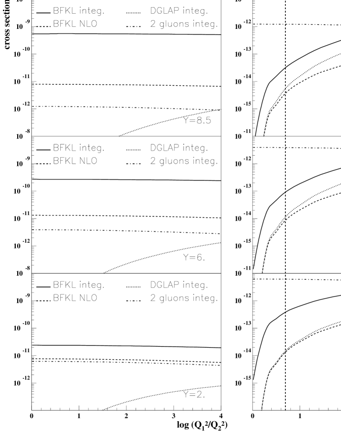
Figure 2: Differential cross-sections vs. $\ln Q^{2}_{1}/Q^{2}_{2}$, for different values of $Y$. Exact values are shown as well as saddle-point approximations. The dashed vertical line on the left hand side is the value $Q^{2}_{1}/Q^{2}_{2}=2$.

Figure 2 shows the differential cross-sections in the BFKL, DGLAP Double Leading Logarithm (DLL) and 2-gluon approximation, as a function of $\ln Q^{2}_{1}/Q^{2}_{2}$ and for three values of $Y$. The cross-sections on the left hand side are calculated using the unintegrated exact formulae 2.1, 2.2, and 2.61 for respectively the BFKL, DGLAP (in the double Leading Log approximation) and 2-gluon exchange cross-sections. Also the phenomenological NLO BFKL cross-sections, as detailed in section 4, are given.

We note that the 2-gluon cross-section is almost always dominating the DGLAP one in the Double Leading Log approximation. The saddle point approximation turns out to be a very good approximation for the BFKL cross-section and is not displayed in the figure (saddle-point results are close to the exact calculation up to $5\%$ in the high $Y$ region, and up to 10% at lower $Y$. A similar conclusion was reached in [5]). We note that the difference between the BFKL and 2-gluon cross-sections increase with $Y$.

On the right side of Figure 2, curves for the exact LO and saddle-point (eq. 2.2) DGLAP calculations are shown, as well as the full NNNLO (eq. 2.61) result and the LO (eq. 2.61, $\ln^{3}Q^{2}_{1}/Q^{2}_{2}$ term only) result for the 2-gluon cross-section. Unlike for the BFKL calculation, for the DGLAP case the saddle-point approximation appears to be in worse agreement with the exact calculation, and overestimates the cross-section by one order of magnitude, which is due to the fact that we are far away from the asymptotic regime. The comparison between the DGLAP-DLL and the 2-gluon cross-section in the LO approximation shows that both cross-sections are similar when $Q_{1}$ and $Q_{2}$ are not too different (the dashed line describes the value $Q_{1}^{2}/Q_{2}^{2}=2$), so precisely in the kinematical domain where the BFKL cross-section is expected to dominate. However, when $Q_{1}^{2}/Q_{2}^{2}$ is further away from one, the LO 2-gluon cross-section is lower than the DGLAP one, especially at large $Y$. This suggests that the 2-gluon cross-section could be a good approximation of the DGLAP one if both are calculated at NNNLO and restricted to the region where $Q_{1}^{2}/Q_{2}^{2}$ is close to one. In this paper we will use the exact NNNLO 2-gluon cross-section in the following to evaluate the effect of the non-BFKL background, since the 2-gluon term appears to constitute the dominant part of the DGLAP cross-section in the region $0.5<Q_{1}^{2}/Q_{2}^{2}<2$.

3.3 Integrated cross-sections

In this chapter, we will study the integrated cross-section over the four kinematical variables $y_{1}$, $y_{2}$, $Q_{1}^{2}$, and $Q_{2}^{2}$, for the exact 2-gluon calculation and the saddle point approximation for the BFKL one.

First we study the effect of the choice of parameters to define the perturbative region for our calculations: Table 1 shows the effect of varying the cut on $\mu^{2}$. At the LC, no effect is seen: scattering the incoming leptons above 40 $\,{\mathrm{mrad}}\,$requires high photon virtualities so that the selected region is always in the perturbative domain. Table 2 contains the BFKL and 2-gluon cross-sections for different values of $\kappa$. The BFKL to 2-gluon ratio is enhanced at high $\kappa$. Table 3 contains the BFKL and 2-gluon cross-sections for different values of the range in ratio $Q_{1}^{2}/Q_{2}^{2}$. The BFKL to 2-gluon ratio is rather insensitive to this restriction. The cut on $1/2\leq Q_{1}^{2}/Q_{2}^{2}\leq 2$ also guarantees that the DGLAP contribution can be well approximated by the two gluon contribution.

We note that for the parameter choice in this paper the maximum ratio between the 2-gluon and BFKL cross-sections is about 20 for the nominal energy and angle cuts at the LC and 40 at LEP.

Next we study the effect of the tagged electron energy and angle. Figure 3 shows the importance of tagging electrons down to low energies (see also Table 4). Reaching $10\%$ of the beam energy or less allows to enhance the counting rates significantly; the difference between the BFKL and 2-gluon predictions also increases, improving the detectability of BFKL dynamics. The effect of increasing the LC detector acceptance for electrons scattered under small angles is illustrated in Figure 4 and in Table 5. The plateau seen at low angles results from the kinematical constraints (see paragraph 3.1).

$\mu^{2}$	$\sigma_{BFKL}^{LEP}$	$\sigma_{2g}^{LEP}$	Ratio	$\sigma_{BFKL}^{LC}$	$\sigma_{2g}^{LC}$	Ratio
2	2.89	3.78E-2	76.5	6.2E-2	2.64E-3	23.5
3	0.57	1.35E-2	42.2	6.2E-2	2.64E-3	23.5
4	0.18	6.14E-3	29.3	6.2E-2	2.64E-3	23.5

Table 1: variation of the cut on $\mu^{2}(\mbox{$\,{\mathrm{GeV}}\,$}^{2})$, for LEP and the LC. The detector acceptance is taken into account.

$\kappa$	$\sigma_{BFKL}^{LEP}$	$\sigma_{2g}^{LEP}$	Ratio	$\sigma_{BFKL}^{LC}$	$\sigma_{2g}^{LC}$	Ratio
10	1.23	9.02E-2	13.6	8.8E-2	9.63E-3	9.1
50	0.81	2.81E-2	28.8	7.2E-2	4.17E-3	17.3
100	0.57	1.35E-2	42.2	6.2E-2	2.64E-3	23.5

Table 2: variation of the cut on $\kappa$, for LEP and the LC. The detector acceptance is taken into account.

$Q^{2}_{1}/Q^{2}_{2}$	$\sigma_{BFKL}^{LEP}$	$\sigma_{2g}^{LEP}$	ratio	$\sigma_{BFKL}^{LC}$	$\sigma_{2g}^{LC}$	ratio
0.5-2	0.57	1.35E-2	42.2	6.2E-2	2.64E-3	23.5
0.1-10	1.71	3.94E-2	43.4	0.123	5.65E-3	21.8
0.01-100	2.00	4.59E-2	43.6	0.128	6.03E-3	21.2

Table 3: Integrated cross-sections (pb) for different ranges of $Q^{2}_{1}/Q^{2}_{2}$, at LEP and LC energies. Electrons are detected between 30 and 95 $\,{\mathrm{GeV}}\,$, down to 33 mrad at LEP, and between 50 and 250 GeV, down to 40 mrad at the LC.

Figure 3: Integrated BFKL and 2-gluon cross-sections, at LEP and the LC. Leptons are tagged from $E_{tag}$ up to the beam energy. We take $\theta_{tag}>33\mbox{$\,{\mathrm{mrad}}\,$}$ at LEP, $\theta_{tag}>40\mbox{$\,{\mathrm{mrad}}\,$}$ at the LC.

Figure 4: Integrated BFKL and 2-gluon cross-sections at the LC, for various acceptances. Leptons are tagged between 50 and 250 GeV.

$\theta$	BFKL	2-gluon	ratio
10	6.7	8.1E-2	82.7
15	6.6	7.9E-2	83.5
20	3.3	4.0E-2	82.5
25	1.1	1.7E-2	64.7
30	0.37	8.4E-3	44.0
35	0.14	4.5E-3	31.1
40	6.18E-2	2.6E-3	23.8

Table 4: Integrated BFKL and 2-gluon cross-sections at the LC for different lower cuts on $\theta_{tag}$, for the kinematic range defined in the text

$E$	BFKL	2-gluon	ratio
60-250	5.1E-2	2.4E-3	21.2
50-250	6.2E-2	2.6E-3	23.8
45-250	6.9E-2	2.7E-3	25.6
40-250	7.7E-2	2.8E-3	27.5
35-250	8.8E-2	2.9E-3	30.3
30-250	0.10	3.1E-3	32.3
25-250	0.12	3.2E-3	37.5
20-250	0.14	3.3E-3	42.4

Table 5: Integrated BFKL and 2-gluon cross-sections at the LC for different lower cuts on $E_{tag}$ for the kinematic range defined in the text

Finally, in Table 6 we give the measurable cross-sections for different values of the beam energy. Although the total cross-sections increase with $E_{beam}$, the opposite is observed after taking into account the detector acceptance and the fact that at constant photon virtuality, the scattered electron aligns more and more with the beam direction when $E_{beam}$ increases.

$E_{beam}$	$\sigma_{BFKL}$	$\sigma_{2-gluon}$	ratio
250	6.18E-2	2.64E-3	23.4
500	7.00E-3	5.21E-4	13.4
1000	8.77E-4	9.92E-5	8.8

Table 6: Integrated cross-sections (pb) for different values of $E_{beam}$ (GeV), after imposing $\theta_{tag}>40\mbox{$\,{\mathrm{mrad}}\,$}$ and $E_{tag}>50\mbox{$\,{\mathrm{GeV}}\,$}$.

Assuming an integrated luminosity of $200\mbox{$\,{\mathrm{pb}}\,$}^{-1}$ per experiment at LEP with center-of-mass energies around $190\mbox{$\,{\mathrm{GeV}}\,$}$, BFKL predicts roughly 200 events provided forward leptons are tagged down to $10\mbox{$\,{\mathrm{GeV}}\,$}$, the 2-gluon prediction being 42 times lower. At the LC, with $50\mbox{$\,{\mathrm{fb}}\,$}^{-1}$ at $\sqrt{s}=500\mbox{$\,{\mathrm{GeV}}\,$}$, $E_{tag}>20\mbox{$\,{\mathrm{GeV}}\,$}$ and $\theta_{tag}>40\mbox{$\,{\mathrm{mrad}}\,$}$, we can expect 7500 BFKL events, compared to 24 times less for the 2-gluon contribution. The final results for the cross-sections are also given in Table 9.

4 Phenomenological approach of NLO effects in BFKL equation

In this section we adopt a phenomenological approach to estimate the effects of higher orders. We will generically label these has “NLO-BFKL” calculations.

4.1 Variation of the scale for rapidity

At Leading Order, the rapidity $Y$ is not uniquely defined. In the formula (2.5), it is possible to add a multiplicative constant $\xi$ in front of $\hat{s}$. Only a NLO calculation can fix this constant. Taking the following definition of the rapidity:

$$Y=\ln\frac{\xi\hat{s}}{\sqrt{Q^{2}_{1}Q^{2}_{2}}}$$ (4.62)

we can study the variation of the BFKL and DGLAP cross-sections for different values of $\xi$. The parameter $\xi$ [26] sets the time scale for the formation of the interacting dipoles. It defines the effective total rapidity interval which is $\ln\frac{1}{\sqrt{X_{1}X_{2}}}+\ln\xi$, $\xi$ being not predictable (but of order one) at the Leading Log approximation. The results are given in Table 7. We note a large dependence of the cross-sections on this parameter, and also of the ratio between the BFKL and 2-gluon predictions which vary between 24 and 2.3!

A phenomenological way to determine this factor $\xi$ has been performed in Reference [3], where a four parameter fit of the proton $F_{2}$ structure function measured by the H1 collaboration [31] has been performed using the QCD dipole picture of BFKL dynamics. The parameter $\xi$ has been found to be 1/3. For this particular value, we note that the BFKL to 2-gluon ratio prediction is reduced to a value of 12.

4.2 Effective value for $\alpha_{S}$

It has recently been demonstrated that the NLO corrections to the BFKL equation are large [32]. The main effect is a reduced value of the so called Lipatov exponent in formula 2.1 [30]. A phenomenological way to approach this is to introduce an effective value of the coupling constant which allows to reduce the value of the Lipatov exponent.

In the same 4-parameter fit described above, used to fit inclusive and diffractive data at HERA, as described in [3, 2], the value of the Lipatov exponent $\alpha_{P}$:

$$\alpha_{P}=4\ln 2\frac{\alpha_{S}N_{C}}{\pi}$$ (4.63)

was fitted and found to be 0.282. In this fit, $\alpha_{S}$ was kept constant. This low value of $\alpha_{P}$ leads to a low value of $\alpha_{S}$ close to 0.11. This low value can be explained phenomenologically by the decrease of the Lipatov exponent due to large NLO corrections.

The same idea can be applied phenomenologically for the $\gamma^{*}\gamma^{*}$ cross-section. We first studied the variation of the BFKL cross-section by setting the scale $\mu^{2}$ in $\alpha_{S}$ in the exponential of formula 2.1 to a number and consequently taking $\alpha_{S}$ fixed. The values of $\alpha_{S}$ and of the BFKL cross-sections are given in Table 8. The cross-section is calculated for $\mu^{2}$=10, 100, 1000, and 10000 GeV² (note that for this study the term $\sqrt{Q_{1}^{2}Q_{2}^{2}}$ is suppressed in the expression of $\mu^{2}$). The decrease of the BFKL cross-section is quite significant.

The last effect studied was to use a varying $\alpha_{S}$, and at the same time taking into account the NLO effects described above. For this purpose, we modify the scale in $\alpha_{S}$ so that the effective value of $\alpha_{S}$ for $Q_{1}^{2}=Q_{2}^{2}=25$ GeV² is about $\alpha_{S}(M_{Z})$. The scale $\mu^{2}$ for $\alpha_{S}$ in the exponential is then expressed as follows:

$$\mu^{2}=\zeta\sqrt{Q_{1}^{2}Q_{2}^{2}}.$$ (4.64)

The variation of the BFKL cross-section as a function of $\zeta$ are given in Table 8 for the LC.

Finally, the results of the BFKL and 2-gluon cross-sections are given in Table 7 if we assume both $\zeta$=1000, and $\xi$=1/3 (see paragraph 4.1). The $\zeta$ value corresponds to a value of $\alpha_{S}=0.11$ for $\mu^{2}=10$ GeV². The ratio BFKL to 2-gluon cross-sections is reduced to 2.3 if both effects are taken into account together.

In Table 9, we also give these effects for LEP with the nominal selection and at the LC with a detector with increased angular acceptance. The ratio given is the comparison of the NLO-BFKL and 2-gluon cross-section. In both cases the sensitivity to BFKL effects is increased. The effect on the cross-section from the angular cut for the LC is shown in Figure 4. The column labelled ’LEP*’ gives the results for the kinematic cuts used by the L3-collaboration who have recently presented preliminary results[33]. The cuts are $E_{tag}$ = 30 GeV and $\theta_{tag}>30\mbox{$\,{\mathrm{mrad}}\,$}$ and $\mu^{2}>2$ GeV². For this selected region the difference between NLO-BFKL and 2-gluon cross-section is only a factor of 2.4. A cut on $Q^{2}_{1}/Q^{2}_{2}$, as done for the other calculations in this paper, would help to allow a more precise determination of the 2-gluon ’background’.

In Figure 2 the differential cross-section calculated with the BFKL-NLO parameters $\zeta$=10000, and $\xi$=1/3 is shown. In Figure 4, the result of the NLO calculation as a function of $\theta_{tag}$ is also displayed for the same values of $\zeta$ and $\xi$. An important observation is that the difference between the NLO calculation and the LO BFKL calculation in Figure 2 increases significantly with increasing $Y$. Hence to establish the BFKL effects in data, a study of the energy or $Y$, rather than the comparison with total cross-sections itself, will be crucial. Note that an additional uncertainty in the cross-section calculations is the number of active flavours considered. For this paper 3 quark flavours were considered both for BFKL and 2-gluon calculations. Including charm only as an additional flavour, without taking into account any mass effect, would increase both cross-sections by a factor 2.56. Including charm can be justified for the LC, but some more sophisticated approach could be necessary for LEP energies.

$\xi$	BFKL	2-gluon	ratio
1	6.2E-2	2.64E-3	23.5
0.1	1.6E-2	2.64E-3	6.1
0.01	6.2E-3	2.64E-3	2.3
1/3	3.1E-2	2.64E-3	11.7
1/3*	6.2E-3	2.64E-3	2.3

Table 7: Variation of the scale for rapidity (see text). The last number (referred by 1/3*) takes also NLO effects on $\alpha_{S}$ in the BFKL equation.

Table 8: Variation of the scale for $\alpha_{S}$ (the change is made in the exponential only). In the left table are given the results for a fixed $\alpha_{S}$ (the scale $\mu^{2}$ is given) and in the second table, $\alpha_{S}$ is running with different values of the parameter $\xi$ (see text). For comparison, the 2-gluon cross-section is 2.64 10^-3 pb.

	BFKLLO	BFKLNLO	2-gluon	ratio
LEP	0.57	3.1E-2	1.35E-2	2.3
LEP*	3.9	0.18	6.8E-2	2.6
LC 40 mrad	6.2E-2	6.2E-3	2.64E-3	2.3
LC 20 mrad	3.3	0.11	3.97E-2	2.8

Table 9: Final cross-sections (pb), for selections described in the text.

5 Conclusion

In this paper, we have studied the differences between the 2-gluon and BFKL and DGLAP $\gamma^{*}\gamma^{*}$ cross-sections both at LEP and LC. It turns out that the double leading logarithmic approximation of the DGLAP cross-section is much lower than the 2-gluon one, calculated to NNNLO. The LO BFKL cross-section is much larger than the 2-gluon cross-section. Unfortunately, the higher order corrections of the BFKL equation (which we estimated phenomenologically) are large, and the 2-gluon and BFKL-NLO cross-sections are reduced to a factor two to four. In particular the $Y$ dependence of the cross-section should remain sensitive to BFKL effects, even in the presence of large higher order corrections.

6 Acknowledgements

We like to thank R. Peschanski and J. Bartels and C. Ewerz for many useful discussions. S.W. thanks the Alexander von Humboldt Foundation and the II. Institut für Theoretische Physik, where the first stage of this work has been done, for support.

7 References

References

• [1] V.S. Fadin, E.A. Kuraev and L.N. Lipatov, Phys. Lett. B60 (1975) 50 ;
I.I. Balitsky and L.N. Lipatov, Sov. J. Nucl. Phys. 28 (1978) 822.
• [2] H. Navelet, R. Peschanski, C. Royon, S. Wallon, Phys. Lett. B385 (1996) 357, H. Navelet, R. Peschanski, C. Royon, Phys. Lett. B366 (1996) 329.
• [3] A. Bialas, R. Peschanski, C. Royon, Phys. Rev. D57 (1998) 6899, S. Munier, R. Peschanski, C. Royon, Nucl. Phys. B534 (1998) 297.
• [4] J. Bartels, A. de Roeck, M. Loewe, Z. Phys. C54 (1991) 635.
• [5] J. Bartels, A. De Roeck and H. Lotter, Phys. Lett. B389 (1996) 742-748.
• [6] S.J. Brodsky, F. Hautmann and D.E. Soper, Phys. Rev. Lett. 78 (1997) 803-806.
• [7] A. Bialas, W. Czyz, W. Florkowski, Eur. Phys. J. C2 (1998) 683.
• [8] G. Altarelli and G. Parisi, Nucl. Phys. B126 (1977) 298; V.N. Gribov and L.N. Lipatov, Sov. Journ. Nucl. Phys. 15 (1972) 438 and 675.
• [9] A.H. Mueller, Nucl. Phys. B415 (1994) 373-385.
• [10] A.H. Mueller and B. Patel, Nucl. Phys. B425 (1994) 471-488.
• [11] A.H. Mueller, Nucl. Phys. B437 (1995) 107-126.
• [12] N.N. Nikolaev and B.G. Zakharov, Zeit. für. Phys. C49 (1991) 607-618; Zeit. für Phys. C53 (1992) 331-346; N.N. Nikolaev, B.G. Zakharov and V.R. Zoller, Phys. Lett. B328 (1994) 486-494.
• [13] J. D. Bjorken, J. B. Kogut, D. E. Soper, Phys. Rev. D3 (1971) 1382.
• [14] L. Landau and E.M. Lifshitz, Relativistic Quantum Theory, Pergamon Press (1971) 351.
• [15] S. Wallon, Thèse de Doctorat, Orsay, 1996.
• [16] H. Navelet and S. Wallon, Nucl. Phys. B522 (1998) 237.
• [17] S. Munier and R. Peschanski, Nucl. Phys. B524 (1998) 377.
• [18] S. Catani, M. Ciafaloni and F. Hautmann, Phys. Lett. B242 (1990) 97; S. Catani, M. Ciafaloni and F. Hautmann, Nucl. Phys. B366 (1991) 135-188; S. Catani and F. Hautmann, Phys. Lett. B315 (1993) 157-163; Nucl. Phys. B427 (1994) 475-524; M. Ciafaloni, Phys. Lett. B356 (1995) 74-78.
• [19] J.C. Collins and R.K. Ellis, Nucl. Phys. B360 (1991) 3-30;
• [20] E.M. Levin, M.G. Ryskin. Yu.M. Shabelskii and A.G. Shuvaev, Sov. J. Nucl. Phys 53 (1995) 657-667.
• [21] A.H. Mueller and G.P. Salam, Nucl. Phys B475 (1996) 293-320.
• [22] Y. Kovchegov, A.H. Mueller and S. Wallon, Nucl. Phys. B507 (1997) 367-378.
• [23] L.N. Lipatov, Sov. Phys. JETP 63 (5) (1986) 904-912.
• [24] A.M. Polyakov, JETP Let. 12 (1970) 381-383.
• [25] I.M. Gel’fand, M.I. Graev, N.Ya. Vilenkin, Generalized Functions (vol 5) Integral Geometry and Representation Theory, Academic Press, New York (1966); C. Itzykson, Quelques aspects de la théorie des groupes, Lectures notes for the Mathematical Physics School of Toulouse University (1974) (in french).
• [26] A. Bialas, Acta Phys. Pol. B28 (1997) 1239.
• [27] H. Navelet, R. Peschanski, C. Royon, L. Schoeffel and S. Wallon, Mod. Phys. Lett. A12 (1997) 887-897.
• [28] G.P. Lepage, P.B. Mackenzie, Phys. Rev. D48 (1993) 2250, S.J. Brodsky, G.P. Lepage, P.B. Mackenzie, Phys. Rev. D28 (1983) 228.
• [29] Conceptual Design of a 500 GeV $e^{+}e^{-}$ Linear Collider with Integrated X-ray Facility, DESY 97-048, ECFA 97-182
• [30] G.P. Salam, J. High Energy Phys. 9807 (1998) 19.
• [31] H1 Coll., Nucl. Phys. B470 (1996) 3.
• [32] V.S. Fadin, L.N. Lipatov, Phys. Lett. B429 (1998) 127.
• [33] Chu Lin, contributed talk at HADRON98, Stara Lesna, September 1998;
M. Kienzle, contributed talk at the 2-photon workshop, Lund, September 1998.