Susy Virtual effects at LEP2 Boundary
Abstract
We examine the possibility that SUSY particles are light, i.e. have a mass just beyond the final kinematical reach of LEP2. In this case, even if light particles are not directly detected, their virtual effects are enhanced by a “close to threshold” resonance in the s-channel. We find that this resonant effect is absent in the case of light sfermions, while it is enhanced in the case of light gauginos, since neutralinos and charginos add coherently in some regions of the allowed parameter space. We discuss this “virtual-alliance” in detail and try to examine the possibilities of its experimental verification.
One of the most interesting sectors of the experimental program at LEP2 [1] is the search for supersymmetric particles. In the specific case of the lightest Higgs boson, these efforts are particularly supported by the existence, within a large class of supersymmetric models [2], of an upper bound of approximately 130-150 GeV that is not much beyond the final kinematical reach ( 100-110 GeV) of the accelerator. This has motivated the rigorous and detailed study of the production mechanism and of its visible manifestations that has been fully illustrated in several dedicated references [3]. Since the nature of the light Higgs couplings with the SM gauge bosons and light fermions makes the detection of virtual effects at one loop rather remote, not much effort has been concentrated on this alternative possibility.
For what concerns the remaining supersymmetric particles, the situation appers to us slightly different. In fact, no definite rigorous upper bound exists on their masses; one can only expect from reasonable arguments based on “naturalness” requests [4] that a limit of a few hundred GeV should not be violated. On the other hand, the possibility of small but visible virtual effects is not, a priori, unconceivable. In particular, the existence of SUSY particles with a mass just beyond the LEP2 reach could be observed as a consequence of a resonant enhancement of self-energies, vertices or boxes due to the production threshold of couples of these particles in the -channel. Note that this remark is far from being obvious because, in principle, the separate enhancements coming from the different diagrams could well interfere destructively and lead to an unobservable effect.
The aim of this paper is precisely that of showing that a specially favourable situation is provided by the hypothetical existence of a light chargino with a mass “close” to 100 GeV (in our analysis we shall assume that the kinematical reach of LEP2 is 200 GeV; this assumption can be easily modified if this turned out to be a pessimistic -or optimistic- input). In such a case, the overall virtual contributions of self-energies, vertices and box origin from chargino pairs to several observables will not be negligible. On top of this, for a large sector of the parameter space of the considered model, an important extra help will come from the simultaneous resonance of virtual neutralinos, whose effect will add coherently with that of the charginos. This kind of “virtual alliance” would lead to small, but observable effects, that we shall discuss here in some detail. As we shall show in the second part of the paper, the effects would be completetly different in the case of virtual contributions due to light sfermions since, owing to the zero spin of the involved particles, the resonant mechanism is practically absent. Therefore, the light chargino-neutralino contribution appears to be a reasonably well identifiable one, in this special and favorable case. We shall devote the first part of this short paper to a detailed numerical analysis of this effect.
To begin our investigation, we shall choose the relevant observables that might be used as indicators of (small) virtual SUSY effects. By definition, these observables must be those that will be measured at LEP2 with the best experimental accuracy, and for which an extremely accurate theoretical prediction within the SM is obviously available. In practice, these requests select three optimal candidates i.e. the muon production cross section , the related forward backward asymmetry and the cross section for hadronic (u, d, s, c, b) production . For these quantities we shall assume the expected experimental precision quoted in the recent dedicated Workshop [1], which amounts roughly to less than a relative one percent, keeping in mind that this value might be (hopefully) improved.
To proceed in a rigorous and self-contained way, we have decided to evaluate both the SM prediction and the SUSY virtual effect using the same computational program. With this purpose, we have first carried on the SM analysis using the semianalytic program PALM, that was illustrated in a previous paper to which we defer for all the technical details [5]. In a second step, we have added to the theoretical PALM SM prediction, computed at the one loop level, the extra virtual SUSY effects. This has been done in a consistent way by adding to the special, gauge invariant combinations of self-energies, vertices and boxes that were grouped in the SM calculation the corresponding SUSY contributions. Technically speaking, this corresponds to adding systematically finite SUSY quantities since all contributions in our approach are subtracted at the peak, . We do not insist here on these details since they can be already found in Ref. [5] for what concerns the SM calculation; the discussion of the SUSY virtual effects at one loop, at general values (here we only consider the LEP2 boundary situation, GeV ) will be given in a more exhaustive forthcoming paper [6].
The theoretical model that we have considered is the MSSM [7], whose detailed discussion we omit. Our starting assumption has been the existence of a light chargino with a mass “just” beyond the LEP2 reach. Obviously, this input can (and will) be easily modified but we shall use it in a first qualitative investigation. We have assumed the GUT relation between the SU(2) U(1) gauginos soft mass parameters to be satisfied [7]. In our simplified approach we neglect left-right mixing in the sfermion mass matrices and we take all physical slepton masses to be degenerate at a common value and all squarks masses degenerate at , and we shall return on this point in the final comments. We also take initial and final state fermions to be massless; this is justified at the c.m. energies that we consider since we cannot have the top as final state. Fixing the mass of the lightest chargino, varies accordingly as a function of the supersymmetric Higgs mass parameter . Gluinos are assumed to be so heavy that they are decoupled. This is justified by recent bounds from hadronic colliders [8]; moreover we are interested here in new physics coming from the weak SU(2) sector of MSSM. Contributions coming from gluinos will be considered in a subsequent paper [6].
Our approach is based on a theoretical description of the invariant scattering amplitude at one loop of the process that uses, as experimental input parameters, quantities that are measured (apart from the electric charge ) on top of the resonance, as discussed in previous papers [9]. In terms of the differential cross section for the corresponding process, this leads to the following expression:
| (1) |
with
| (5) | |||||
| (9) | |||||
where is the conventional color factor which contains standard QCD corrections at variable , and where the theoretical input in Eqs. (5-9) contains the partial leptonic and (light) hadronic widths , and the related weak effective angles , () measured on top of the resonance [9]. The functions that appear in the brackets are defined as follows:
| (11) |
| (12) |
| (13) |
| (14) |
where
| (15) |
| (16) |
| (17) |
| (18) |
| (20) | |||||
| (22) | |||||
The quantities () are the conventional transverse self-energies. are the projections on the photon and Lorentz structures of the box contributions to the scattering amplitude and the various brackets () are the projections of the vertices on the different Lorentz structures to which , , , belong. In our notations is the component of the scattering amplitude at one loop that appears in the form where is what we call the photon Lorentz structure and analogous definitions are obtained for , , with the Lorentz structure defined as .
More details can be found e.g. in [5]. Here we only stress the fact that all the previous quantities , , , are separately gauge-invariant and therefore their evaluation in the SM can be performed without intrinsic ambiguities, leading to the numerical results fully discussed in [5].
To compute the SUSY effect on the three chosen observables, we have calculated the quantities , , , . These are finite contributions that are generated by Feynman diagrams of self energy, vertex and box type. In Figs. (1,2,3) we represent diagrammatically some of the relevant graphs, omitting for simplicity other ones e.g. external self-energy insertions. As a technical comment, we would like to note that one could expect various Lorentz-invariant Dirac structures to contribute to the amplitudes under consideration, especially in the case of SUSY boxes that have a non conventional structure with respect to the SM ones. However, due to a “generalized Fierz identity” that will be discussed in detail elsewhere [6], it is possible to demonstrate that only four independent Dirac structures (i.e., where are the chiral projectors) contribute in the massless external fermions case that we consider here.
Inserting the expressions of the SUSY contribution to Eqs. (11-14) into the general equations (1)-(9) and performing the angular integration by means of the PALM program we have computed the overall (SM) and (SM+MSSM) values. Although the program is able to estimate ISR (Initial State Radiation) effects [5], we have not inserted for our present investigation at GeV the discussion of this kind of effects; we believe that for the purposes of this preliminary investigation this attitude can be safely tolerated.
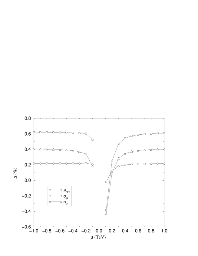
We have first considered a case in which the light chargino mass is fixed at 105 GeV, the sleptons physical masses are equal to 120 GeV and the squarks physical ones are assumed to be 200 GeV. We set , and verified that varying it from 1.6 to 40 does not produce any appreciable change. With this choice, we computed the relative SUSY shifts on the three chosen observables , ().
Fig. (4) shows the variations of the relative effects on the observables when GeV and varies in its allowed range. One sees that the size of the SUSY contribution to the muon asymmetry remains systematically negligible, well below the six-seven permille limit that represents an optimistic experimental reach in this case [1]. The weakness of this effect is due to two facts, the dominance of the photon contribution in and of the photon- interference in , and a subsequent accidental cancellation between and in the resulting + contribution to . On the contrary, in the case of the muon and hadronic cross sections, the size of the effect approaches, for large values, a limit of six permille in and four permille in that represent a conceivable experimental reach, at the end of the overall LEP2 running period.
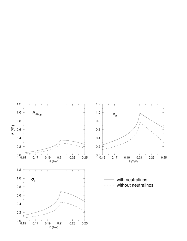
This explains in fact our choice of the value GeV with LEP2 limit at 200 GeV; other couples of the light chargino mass and of the LEP2 limit separated by a larger gap would produce a smaller effect, i.e. an unobservable one. On the other hand, smaller gaps (e.g. a lighter but still unproduced chargino or a larger LEP2 limit) would increase the effect, as one see in Fig. (5), towards the one percent values that appear to be experimentally realistic.
Let us now discuss the qualitative features of the results that we obtain. As one sees from Fig. (6), the one loop SUSY effects have different signatures. Those of “oblique” (universal) type, corresponding to self-energies, have a negative effect on all three observables; those of non-universal type (vertices and boxes) lead to a positive one in all the three cases. Now, when we have a light “gaugino like” chargino of a (fixed) mass 105 GeV , and a heavy “higgsino like” chargino of a mass of the order of itself. At the same time, in the neutralino sector the situation is very similar, with two heavy “higgsino like” neutralinos, and two light “gaugino like” neutralinos of masses and . Then, 1 chargino + 1 neutralino are “gaugino like” and have roughly the same mass of order GeV “resonating” coherently in the vertex, box and self-energies contributions. This situation, which we call of “virtual alliance”, is made evident in Fig. (7) where neutralinos are seen to contribute for about 25 % ot the total signal. Note that an important contribution to the overall effect in the chosen configuration is that coming from the SUSY boxes[10].
The opposite happens when . In this situation we have light “higgsino type” charginos and neutralinos, with masses of the order 105 GeV, and heavy “gaugino type” charginos and neutralinos. Since higgsinos are decoupled from massless fermions, their contribution to boxes and vertices disappear and the overall signal is consequently weakened (see Fig.(5)).
Let us now consider a different situation, where the lightest chargino is “heavy” and decoupled, setting its mass equal to 300 GeV, and assuming that all sleptons are now “light” (i.e. 105 GeV). The analogue of Fig. (6) is then represented in Fig. (8). As one sees from the figure, the signal has now almost completely disappeared. This fact can be qualitatively interpreted as a disappearance of the “quasi resonance” chargino-neutralino contributions, not compensated by analogous sleptons terms. The reason is the fact that spinless particles, differently from spin 1/2 particles, have to be produced because of angular momentum conservation, in a l=1 angular momentum state. This causes a relative “threshold” p-wave depression factor in the spinless case, which washes out the threshold enhancement. Note also that, since we are not considering final electron-positron states, we don’t have any box contributions with sfermions pairs in the s-channel (see Fig. (1)).
Another important comment is related to our choice of using a “Z-peak subtracted” representation. This has the consequence that all the energy independent new physics contributions that can be reabsorbed in the Z-peak input quantities () do not affect our final result. Such is the case for all those values of sfermions splittings and/or mixings that contribute to the parameter . These contributions are automatically reabsorbed when we replace by as theoretical input. They are, though, taken into account by the experimental error on our theoretical input, in this case . As exhaustively discussed in [5] this would generate a strip of theoretical error in our prediction of the one permille size well below the considered LEP2 experimental accuracy.
Note that, as a consequence of this “LEP1 based” approach, all our residual subtracted theoretical one-loop combinations of self energies, vertices and boxes are finite and thus separately computable. In a forthcoming paper [6] we shall discuss in more detail a dedicated numerical code (SPALM), that is already available upon request.
We should mention at this point that in a recent paper [11] a calculation of virtual SUSY effect has been performed, that covers an energy range from to the range. The approach followed by the authors of Ref.[11] is different from ours, particularly since the theoretical input parameters are different and do not contain our LEP1 input. This makes a detailed comparison more subtle, in particular for what concerns ”relative” shifts when the input parameters are different. Since the ”virtual alliance” case that we considered here has not been treated in Ref.[11], we postpone a complete and clean comparison of the two approaches to the forthcoming paper [6].
In conclusion, we have seen that in the large configuration, a delicate interplay exists between virtual SUSY contributions from self-energies, vertices and boxes that might lead, for a conveniently light chargino, to a small but visible effect. Our prediction is that the signature of the effect is a positive shift of the muonic and hadronic cross sections. Given the relative smallness of the signal, an important help comes from the light neutralino, in particular from its box contribution that adds coherently to that of the chargino, giving a 25 % enhancement of the signal. This can be interpreted as a kind of “virtual alliance”, as we anticipated in the abstract. The observation of the predicted simultaneous small excess in the two cross sections, typically at the 1 % level at most, could well be within the reach of a series of dedicated LEP2 experiments.
REFERENCES
- [1] Physics at LEP2, Proceedings of the Workshop-Geneva, Switzerland (1996), CERN 96-01, G. Altarelli, T. Sjostrand and F. Zwirner eds.
- [2] M. Quiros, J. R. Espinosa (CERN). CERN-TH-98-292, 1998, Presented at 6th International Symposium on Particles, Strings and Cosmology (PASCOS 98), Boston, MA, 22-27 Mar 1998; e-Print Archive: hep-ph/9809269 and references therein.
- [3] Physics at LEP2, Search for New Physics, Proceedings of the Workshop-Geneva, Switzerland (1996), CERN 96-01, p.46, G. Altarelli, T. Sjostrand and F. Zwirner eds.
- [4] R. Barbieri, G.F. Giudice, Nucl.Phys.B306,63(1988); G.W. Anderson, D.J. Castano, Phys.Lett.B347,300(1995); P. Ciafaloni and A. Strumia, Nucl. Phys. B494,41(1997); L. Giusti, A. Romanino, A. Strumia, IFUP-TH-49-98, Nov 1998; e-Print Archive: hep-ph/9811386.
- [5] M. Beccaria, G. Montagna, F. Piccinini, F.M. Renard, C. Verzegnassi, Phys.Rev. D58,093014(1998).
- [6] M. Beccaria, P. Ciafaloni, D. Comelli, F. Renard, C. Verzegnassi, “A Z-peak subtracted analysis of virtual SUSY effects at future colliders”, in preparation.
- [7] H.P. Nilles, Phys.Rep. 110,1(1984); H.E. Haber and G.L. Kane, Phys. Rep. 117,75(1985); R. Barbieri, Riv.Nuov.Cim. 11,1(1988); R. Arnowitt, A, Chamseddine and P. Nath, ”Applied N=1 Supergravity (World Scientific, 1984); for a recent review see e.g. S.P. Martin, hep-ph/9709356.
- [8] Particle data group 1998, European Physical Journal C3 (1998) 1.
- [9] F.M. Renard, C. Verzegnassi, Phys. Rev. D52, 1369 (1995); Phys. Rev. D53,1290(1996).
- [10] J. Layssac, F.M. Renard and C. Verzegnassi, Phys. Lett.B418,134(1998).
- [11] W. Hollik, C. Schappacher, hep-ph/9807427.