Abstract

We present detailed results of a diagrammatic calculation of the leading two-loop QCD corrections to the masses of the neutral ${\cal CP}$-even Higgs bosons in the Minimal Supersymmetric Standard Model (MSSM). The two-loop corrections are incorporated into the full diagrammatic one-loop result and supplemented with refinement terms that take into account leading electroweak two-loop and higher-order QCD contributions. The dependence of the results for the Higgs-boson masses on the various MSSM parameters is analyzed in detail, with a particular focus on the part of the parameter space accessible at LEP2 and the upgraded Tevatron. For the mass of the lightest Higgs boson, $m_{h}$, a parameter scan has been performed, yielding an upper limit on $m_{h}$ which depends only on $\tan\beta\hskip 2.84526pt$. The results for the Higgs-boson masses are compared with results obtained by renormalization group methods. Good agreement is found in the case of vanishing mixing in the scalar quark sector, while sizable deviations occur if squark mixing is taken into account.

1 Introduction

The search for the lightest Higgs boson is a crucial test of Supersymmetry (SUSY) which can be performed with the present and the next generation of accelerators. The prediction of a relatively light Higgs boson is common to all supersymmetric models whose couplings remain in the perturbative regime up to a very high energy scale [1]. A precise prediction for the mass of the lightest Higgs boson in terms of the relevant SUSY parameters is necessary in order to determine the discovery and exclusion potential of LEP2 and the upgraded Tevatron, and for physics at the LHC and future linear colliders, where eventually a high-precision measurement of the mass of this particle might be possible. A precise knowledge of the mass of the heavier ${\cal CP}$-even Higgs boson, $m_{H}$, is important for resolving the mass splitting between the ${\cal CP}$-even and -odd Higgs-boson masses.

In the Minimal Supersymmetric Standard Model (MSSM) [2] at the tree level the mass $m_{h}$ of the lightest Higgs boson is restricted to be smaller than the $Z$-boson mass. However, this bound is strongly affected by the inclusion of radiative corrections: the dominant one-loop corrections arise from the top and scalar-top loops which yield terms of the form $G_{F}m_{t}^{4}\ln(m_{\tilde{t}_{1}}m_{\tilde{t}_{2}}/m_{t}^{2})$ [3]. These results have been improved by performing a complete one-loop calculation in the on-shell scheme, which takes into account the contributions of all sectors of the MSSM [4, 5, 6]. Beyond one-loop order, renormalization group (RG) methods have been applied in order to include leading logarithmic higher-order contributions [7, 8, 9, 10]. In the effective potential approach diagrammatic results for the dominant two-loop contributions have been obtained in the limiting case of vanishing $\tilde{t}$-mixing and infinitely large $M_{A}$ and $\tan\beta\hskip 2.84526pt$ [11]. The calculation of the leading QCD corrections in this approach has recently been generalized to the case of arbitrary $\tan\beta\hskip 2.84526pt$ and non-vanishing $\tilde{t}$-mixing [12].

Up to now phenomenological analyses have been based either on the RG results [7, 8, 9, 10], or on the complete one-loop on-shell results [4, 5, 6]. These results differ by large leading logarithmic higher-order contributions, which are not included in the one-loop on-shell results, but also by non-leading one-loop contributions, which are neglected in the RG approach. The numerical difference in the Higgs-mass predictions between the two approaches reaches up to 20 GeV.

Recently a Feynman-diagrammatic calculation of the leading two-loop corrections of ${\cal O}(\alpha\alpha_{s})$ to the masses of the neutral ${\cal CP}$-even Higgs bosons has been performed [13, 14]. Compared to the leading one-loop result the two-loop contribution was found to give rise to a considerable reduction of the $m_{h}$ value. The leading two-loop corrections have been combined with the full diagrammatic one-loop on-shell result [5] and further refinements have been included concerning the leading two-loop Yukawa corrections of ${\cal O}(G_{F}^{2}m_{t}^{6})$ [8, 15] and leading QCD corrections beyond two-loop order.

In this paper we present in detail the steps of this calculation. The results for the masses of the neutral ${\cal CP}$-even Higgs bosons are analyzed in terms of the relevant parameters of the MSSM. A parameter scan for the lightest Higgs-boson mass is performed yielding an upper bound for $m_{h}$ within the MSSM (apart from certain threshold regions which correspond to very specific configurations of the MSSM parameters) given exclusively in terms of $\tan\beta\hskip 2.84526pt$. This upper bound is discussed in view of the discovery potential of LEP2 and the upgraded Tevatron. The results for $m_{h}$ are compared with the corresponding results obtained by RG methods. The comparison is performed both in terms of the (unobservable) parameters of the scalar top mass matrix and in terms of the physical stop masses and the stop mixing angle.

The paper is organized as follows: Section 2 contains our notations and a description fo the renormalization procedure as required for the corrections in the MSSM Higgs sector in ${\cal O}(\alpha\alpha_{s})$. The main features of the calculation are discussed in section 3. In section 4 we present a detailed numerical analysis of the results for the neutral ${\cal CP}$-even Higgs-boson masses as functions of the different SUSY parameters. We perform a scan for $m_{h}$ over the parameters $m_{\tilde{g}},M_{A},M,\mu$ and the $\tilde{t}$-mixing parameter and determine the maximal possible values of $m_{h}$ as a function of $\tan\beta\hskip 2.84526pt$. Finally numerical comparisons are shown with results obtained by renormalization group (RG) methods. In section 5 we give our conclusions.

2 Renormalization

2.1 The Higgs sector of the MSSM

The Higgs sector of the MSSM consists of two Higgs doublets $H_{1}$, $H_{2}$ with opposite hypercharges $Y_{1}=-1$ and $Y_{2}=+1$ and non-vanishing vacuum expectation values $v_{1}$ and $v_{2}$. The Higgs doublets can be decomposed according to

$$H_{1} = \left(\begin{array}[]{c}H_{1}^{0}\\[2.15277pt] H_{1}^{-}\end{array}\right)\;=\;\left(\begin{array}[]{c}v_{1}+\frac{1}{\sqrt{2}}(\phi_{1}^{0}+i\chi_{1}^{0})\\[2.15277pt] -\phi_{1}^{-}\end{array}\right)$$ (5)

$$H_{2} = \left(\begin{array}[]{c}H_{2}^{+}\\[2.15277pt] H_{2}^{0}\end{array}\right)\;=\;\left(\begin{array}[]{c}\phi_{2}^{+}\\[2.15277pt] v_{2}+\frac{1}{\sqrt{2}}(\phi_{2}^{0}+i\chi_{2}^{0})\end{array}\right)~{}.$$ (10)

The vacuum expectation values define the angle $\beta$ via

$$\tan\beta\hskip 2.84526pt\equiv\frac{v_{2}}{v_{1}};\qquad 0<\beta<\pi/2~{}.$$ (11)

The Higgs potential, including all soft SUSY breaking terms reads [16] ($\epsilon_{12}=-1$):

$$V = m_{1}^{2}|H_{1}|^{2}+m_{2}^{2}|H_{2}|^{2}-m_{12}^{2}(\epsilon_{ab}H_{1}^{a}H_{2}^{b}+\mbox{h.c.})$$ (12)

$$+\frac{1}{8}({g_{1}}^{2}+{g_{2}}^{2})\left[|H_{1}|^{2}-|H_{2}|^{2}\right]^{2}+\frac{1}{2}{g_{2}}^{2}|H_{1}^{{\dagger}}H_{2}|^{2}~{},$$

where $m_{i}^{2}\equiv|\mu|^{2}+\tilde{m}_{i}^{2}\;(i=1,2)$; $\tilde{m}_{1}$, $\tilde{m}_{2}$, $m_{12}$ are the soft SUSY breaking terms, and $\mu$ denotes the mixing between $H_{1}$ and $H_{2}$. The coupling constants of the Higgs self-interaction are, contrary to the SM, determined through the gauge coupling constants $g_{1}$ and $g_{2}$. Besides $g_{1}$, $g_{2}$ two independent parameters are required to fix the potential (12) at the tree level. Conventionally they are chosen as $\tan\beta\hskip 2.84526pt$ and $M_{A}^{2}=-m_{12}^{2}(\tan\beta\hskip 2.84526pt+\cot\beta\hskip 2.84526pt)$, where $M_{A}$ is the mass of the ${\cal CP}$-odd $A$ boson.

The diagonalization of the bilinear part of the Higgs potential, i.e. the Higgs mass matrices, is performed via the orthogonal transformations

$$\left(\begin{array}[]{c}H^{0}\\[2.15277pt] h^{0}\end{array}\right) = \left(\begin{array}[]{cc}\cos\alpha&\sin\alpha\\[2.15277pt] -\sin\alpha&\cos\alpha\end{array}\right)\left(\begin{array}[]{c}\phi_{1}^{0}\\[2.15277pt] \phi_{2}^{0}\end{array}\right)$$ (19)

$$\left(\begin{array}[]{c}G^{0}\\[2.15277pt] A^{0}\end{array}\right) = \left(\begin{array}[]{cc}\cos\beta&\sin\beta\\[2.15277pt] -\sin\beta&\cos\beta\end{array}\right)\left(\begin{array}[]{c}\chi_{1}^{0}\\[2.15277pt] \chi_{2}^{0}\end{array}\right)$$ (26)

$$\left(\begin{array}[]{c}G^{\pm}\\[2.15277pt] H^{\pm}\end{array}\right) = \left(\begin{array}[]{cc}\cos\beta&\sin\beta\\[2.15277pt] -\sin\beta&\cos\beta\end{array}\right)\left(\begin{array}[]{c}\phi_{1}^{\pm}\\[2.15277pt] \phi_{2}^{\pm}\end{array}\right)~{},$$ (33)

with $\beta$ from eq. (11). The mixing angle $\alpha$ is determined through

$$\tan 2\alpha=\tan 2\beta\;\frac{M_{A}^{2}+M_{Z}^{2}}{M_{A}^{2}-M_{Z}^{2}};\qquad-\frac{\pi}{2}<\alpha<0~{}.$$ (34)

One gets the following Higgs spectrum:

$$\mbox{2 neutral bosons},\,{\cal CP}=+1 : h^{0},H^{0}$$

$$\mbox{1 neutral boson},\,{\cal CP}=-1 : A^{0}$$

2 charged bosons $$: H^{+},H^{-}$$

3 unphysical Goldstone bosons $$: G^{0},G^{+},G^{-}.$$ (35)

The masses of the gauge bosons are given in analogy to the SM:

$$M_{W}^{2}=\frac{1}{2}g_{2}^{2}(v_{1}^{2}+v_{2}^{2});\qquad M_{Z}^{2}=\frac{1}{2}(g_{1}^{2}+g_{2}^{2})(v_{1}^{2}+v_{2}^{2});\qquad M_{\gamma}=0.$$ (36)

At tree level the mass matrix of the neutral ${\cal CP}$-even Higgs bosons is given in the $\phi_{1}$-$\phi_{2}$-basis in terms of $M_{Z}$, $M_{A}$, and $\tan\beta\hskip 2.84526pt$ by

$$M_{\rm Higgs}^{2,{\rm tree}} = \left(\begin{array}[]{cc}m_{\phi_{1}}^{2}&m_{\phi_{1}\phi_{2}}^{2}\\ m_{\phi_{1}\phi_{2}}^{2}&m_{\phi_{2}}^{2}\end{array}\right)$$ (39)

$$= \left(\begin{array}[]{cc}M_{A}^{2}\sin^{2}\beta\hskip 2.84526pt+M_{Z}^{2}\cos^{2}\beta&-(M_{A}^{2}+M_{Z}^{2})\sin\beta\hskip 2.84526pt\cos\beta\\ -(M_{A}^{2}+M_{Z}^{2})\sin\beta\hskip 2.84526pt\cos\beta&M_{A}^{2}\cos^{2}\beta\hskip 2.84526pt+M_{Z}^{2}\sin^{2}\beta\end{array}\right),$$ (42)

which by diagonalization according to eq. (19) yields the tree-level Higgs-boson masses

$$M_{\rm Higgs}^{2,{\rm tree}}\stackrel{{\scriptstyle\alpha}}{{\longrightarrow}}\left(\begin{array}[]{cc}m_{H,{\rm tree}}^{2}&0\\ 0&m_{h,{\rm tree}}^{2}\end{array}\right)~{}.$$ (43)

In order to slightly simplify the two-loop calculation, we have chosen to perform it in the $\phi_{1}$-$\phi_{2}$-basis. In this way the angle $\alpha$ does not appear in the calculation of the two-loop self-energies, but enters at the end when the rotation into the physical basis is performed.

In order to deal with the arising divergencies and to establish the meaning of the physical parameters beyond the tree level, one has to renormalize the Higgs and the scalar top sector of the MSSM. For the corrections of ${\cal O}(\alpha\alpha_{s})$ to the Higgs-boson masses, in the focus of this discussion here, renormalization up to the two-loop level is needed. In the following we specify the renormalization for the relevant quantities in this calculation (explicitly listed are only those terms that actually contribute at ${\cal O}(\alpha\alpha_{s})$). The renormalization of the complete one-loop contributions to the neutral ${\cal CP}$-even Higgs-boson masses has been performed according to Ref. [5].

We use the following notation: $\Sigma^{(1)}$ and $\Sigma^{(2)}$ denote the one- and two-loop part of an unrenormalized self-energy, $\hat{\Sigma}^{(1)}$ and $\hat{\Sigma}^{(2)}$ denote the one- and two-loop part of a renormalized self-energy, and $\Sigma^{\prime}(k^{2})=\frac{\partial}{\partial k^{2}}\Sigma(k^{2})$. $t_{1}$ and $t_{2}$ denote the unrenormalized tadpoles; $t^{(1)}$ and $t^{(2)}$ represent the one- and two-loop part of an unrenormalized tadpole, and $\hat{t}_{1},\hat{t}_{2}$ denote the renormalized tadpoles.

The renormalization of the masses and fields is performed as follows:

$$M_{Z}^{2} \to M_{Z}^{2}+\delta M_{Z}^{2\,(1)}+\delta M_{Z}^{2\,(2)},$$ (44)

$$M_{A}^{2} \to M_{A}^{2}+\delta M_{A}^{2\,(1)}+\delta M_{A}^{2\,(2)},$$ (45)

$$\varphi_{1} \to \varphi_{1}Z_{H_{1}}^{1/2},\quad\varphi_{1}=\phi_{1}^{0},\chi_{1}^{0},\phi_{1}^{-},$$ (46)

$$\varphi_{2} \to \varphi_{2}Z_{H_{2}}^{1/2},\quad\varphi_{2}=\phi_{2}^{0},\chi_{2}^{0},\phi_{2}^{+},$$ (48)

$$Z_{H_{i}}=1+\delta Z_{H_{i}}^{(1)}+\delta Z_{H_{i}}^{(2)}$$

$$\tan\beta\hskip 2.84526pt \to \tan\beta\hskip 2.84526pt(1+\delta\tan\beta\hskip 2.84526pt^{(1)}+\delta\tan\beta\hskip 2.84526pt^{(2)}),$$ (49)

$$t_{i} \to t_{i}+\delta t_{i}^{(1)}+\delta t_{i}^{(2)}~{}~{}(i=1,2)~{}.$$ (50)

This yields for the renormalized two-loop self-energies of $\phi_{1}$ and $\phi_{2}$:

$$\hat{\Sigma}^{(2)}_{\phi_{1}}(k^{2}) = \Sigma^{(2)}_{\phi_{1}}(k^{2})+k^{2}\delta Z_{H_{1}}^{(2)}-\delta V_{\phi_{1}}^{(2)},$$ (51)

$$\hat{\Sigma}^{(2)}_{\phi_{2}}(k^{2}) = \Sigma^{(2)}_{\phi_{2}}(k^{2})+k^{2}\delta Z_{H_{2}}^{(2)}-\delta V_{\phi_{2}}^{(2)},$$ (52)

$$\hat{\Sigma}^{(2)}_{\phi_{1}\phi_{2}}(k^{2}) = \Sigma^{(2)}_{\phi_{1}\phi_{2}}(k^{2})-\delta V_{\phi_{1}\phi_{2}}^{(2)},$$ (53)

where it is understood that the unrenormalized self-energies at two-loop order also contain the contributions arising from the subloop renormalization. The expressions $\delta V_{\phi_{1}}^{(2)},\delta V_{\phi_{2}}^{(2)}$ and $\delta V_{\phi_{1}\phi_{2}}^{(2)}$ are the two-loop counterterm contributions from the Higgs potential:

$$\delta V_{\phi_{1}}^{(2)} = \delta M_{Z}^{2\,(2)}\cos^{2}\beta\hskip 2.84526pt+\delta M_{A}^{2\,(2)}\sin^{2}\beta\hskip 2.84526pt-\delta t_{1}^{(2)}\frac{e}{2M_{W}s_{W}}\cos\beta\hskip 2.84526pt(1+\sin^{2}\beta\hskip 2.84526pt)$$ (54)

$$+\delta t_{2}^{(2)}\frac{e}{2M_{W}s_{W}}\cos^{2}\beta\hskip 2.84526pt\sin\beta\hskip 2.84526pt+\delta Z_{H_{1}}^{(2)}\left(M_{Z}^{2}\cos^{2}\beta\hskip 2.84526pt+M_{A}^{2}\sin^{2}\beta\hskip 2.84526pt\right)$$

$$+\delta\tan\beta\hskip 2.84526pt^{(2)}\cos^{2}\beta\hskip 2.84526pt\sin^{2}\beta\hskip 2.84526pt(M_{A}^{2}-M_{Z}^{2}),$$

$$\delta V_{\phi_{2}}^{(2)} = \delta M_{Z}^{2\,(2)}\sin^{2}\beta\hskip 2.84526pt+\delta M_{A}^{2\,(2)}\cos^{2}\beta\hskip 2.84526pt-\delta t_{2}^{(2)}\frac{e}{2M_{W}s_{W}}\sin\beta\hskip 2.84526pt(1+\cos^{2}\beta\hskip 2.84526pt)$$ (55)

$$+\delta t_{1}^{(2)}\frac{e}{2M_{W}s_{W}}\sin^{2}\beta\hskip 2.84526pt\cos\beta\hskip 2.84526pt+\delta Z_{H_{2}}^{(2)}\left(M_{Z}^{2}\sin^{2}\beta\hskip 2.84526pt+M_{A}^{2}\cos^{2}\beta\hskip 2.84526pt\right)$$

$$-\delta\tan\beta\hskip 2.84526pt^{(2)}\cos^{2}\beta\hskip 2.84526pt\sin^{2}\beta\hskip 2.84526pt(M_{A}^{2}-M_{Z}^{2}),$$

$$\delta V_{\phi_{1}\phi_{2}}^{(2)} = -\delta M_{Z}^{2\,(2)}\sin\beta\hskip 2.84526pt\cos\beta\hskip 2.84526pt-\delta M_{A}^{2\,(2)}\sin\beta\hskip 2.84526pt\cos\beta\hskip 2.84526pt-\delta t_{1}^{(2)}\frac{e}{2M_{W}s_{W}}\sin^{3}\beta\hskip 2.84526pt$$ (56)

$$-\delta t_{2}^{(2)}\frac{e}{2M_{W}s_{W}}\cos^{3}\beta\hskip 2.84526pt-\delta Z_{H_{1}}^{(2)}\frac{\sin\beta\hskip 2.84526pt\cos\beta\hskip 2.84526pt}{2}\left(M_{A}^{2}-M_{Z}^{2}\right)$$

$$-\delta Z_{H_{2}}^{(2)}\frac{\sin\beta\hskip 2.84526pt\cos\beta\hskip 2.84526pt}{2}\left(M_{A}^{2}-M_{Z}^{2}\right)$$

$$-\delta\tan\beta\hskip 2.84526pt^{(2)}\frac{1}{2}\sin 2\beta\hskip 2.84526pt\cos 2\beta\hskip 2.84526pt(M_{A}^{2}+M_{Z}^{2}),$$

with the electroweak mixing angle $s_{W}^{2}=1-c_{W}^{2}$, $c_{W}^{2}=M_{W}^{2}/M_{Z}^{2}$.

The counterterms are fixed by imposing on-shell renormalization conditions for the renormalized self-energies. For the $A$ boson this reads:

$$\mbox{Re}\,\hat{\Sigma}_{A}(M_{A}^{2})=0~{}.$$ (57)

The tadpole conditions are:

$$\hat{t}_{1}=0,\quad\hat{t}_{2}=0~{}.$$ (58)

The conditions for the tadpoles have the consequence that the $v_{i}$ remain the minima of the Higgs potential also at the two-loop level.

The resulting expressions for the renormalization constants contributing to the leading two-loop corrections to the neutral ${\cal CP}$-even Higgs-boson masses, expressed in terms of unrenormalized self-energies and tadpoles, are given in Sec. 3.1.

2.2 The scalar quark sector of the MSSM

Renormalization in the squark sector is needed in the present calculation at the one-loop level, i.e. at ${\cal O}(\alpha_{s})$. As above, we work in the on-shell scheme. In the following the formulas are written for one flavor.

The squark mass term of the MSSM Lagrangian is given by

$${\cal L}_{m_{\tilde{f}}}=-\frac{1}{2}\Big{(}\tilde{f}_{L}^{{\dagger}},\tilde{f}_{R}^{{\dagger}}\Big{)}\;{\bf Z}\;\left(\begin{array}[]{c}\tilde{f}_{L}\\[2.15277pt] \tilde{f}_{R}\end{array}\right)~{},$$ (59)

where

$${\bf Z}=\left(\begin{array}[]{cc}M_{\tilde{Q}}^{2}+M_{Z}^{2}\cos 2\beta\hskip 2.84526pt(I_{3}^{f}-Q_{f}s_{W}^{2})+m_{f}^{2}&m_{f}(A_{f}-\mu\{\cot\beta\hskip 2.84526pt;\tan\beta\hskip 2.84526pt\})\\ m_{f}(A_{f}-\mu\{\cot\beta;\tan\beta\})&M_{\tilde{Q}^{\prime}}^{2}+M_{Z}^{2}\cos 2\beta\hskip 2.84526ptQ_{f}s_{W}^{2}+m_{f}^{2}\end{array}\right),$$ (60)

and $\{\cot\beta\hskip 2.84526pt;\tan\beta\hskip 2.84526pt\}$ corresponds to $\{u;d\}$-type squarks. The soft SUSY breaking term $M_{\tilde{Q}^{\prime}}$ is given by:

$$M_{\tilde{Q}^{\prime}} = \left\{\begin{array}[]{cl}M_{\tilde{U}}&\quad\mbox{for right handed $u$-type squarks}\\ M_{\tilde{D}}&\quad\mbox{for right handed $d$-type squarks}\end{array}\right..$$ (63)

In order to diagonalize the mass matrix and to determine the physical mass eigenstates the following rotation has to be performed:

$$\left(\begin{array}[]{c}\tilde{f}_{1}\\ \tilde{f}_{2}\end{array}\right)=\left(\begin{array}[]{cc}\cos\theta\kern-1.99997pt_{\tilde{f}}&\sin\theta\kern-1.99997pt_{\tilde{f}}\\ -\sin\theta\kern-1.99997pt_{\tilde{f}}&\cos\theta\kern-1.99997pt_{\tilde{f}}\end{array}\right)\left(\begin{array}[]{c}\tilde{f}_{L}\\ \tilde{f}_{R}\end{array}\right).$$ (64)

The mixing angle $\theta\kern-1.99997pt_{\tilde{f}}$ is given for $\tan\beta\hskip 2.84526pt>1$ by:

$$\cos\theta\kern-1.99997pt_{\tilde{f}} = \sqrt{\frac{(m_{\tilde{f}_{R}}^{2}-m_{\tilde{f}_{1}}^{2})^{2}}{m_{f}^{2}\,(A_{f}-\mu\{\cot\beta\hskip 2.84526pt;\tan\beta\hskip 2.84526pt\})^{2}+(m_{\tilde{f}_{R}}^{2}-m_{\tilde{f}_{1}}^{2})^{2}}}$$ (65)

$$\sin\theta\kern-1.99997pt_{\tilde{f}} = \mp\;sgn\Big{[}A_{f}-\mu\{\cot\beta\hskip 2.84526pt;\tan\beta\hskip 2.84526pt\}\Big{]}$$ (66)

$$\times\;\sqrt{\frac{m_{f}^{2}\,(A_{f}-\mu\{\cot\beta\hskip 2.84526pt;\tan\beta\hskip 2.84526pt\})^{2}}{m_{f}^{2}\,(A_{f}-\mu\{\cot\beta\hskip 2.84526pt;\tan\beta\hskip 2.84526pt\})^{2}+(m_{\tilde{f}_{R}}^{2}-m_{\tilde{f}_{1}}^{2})^{2}}}~{}.$$

The negative sign in (66) corresponds to $u$-type squarks, the positive sign to $d$-type ones. $m_{\tilde{f}_{R}}^{2}=M_{\tilde{Q}^{\prime}}^{2}+M_{Z}^{2}\cos 2\beta\hskip 2.84526ptQ_{f}s_{W}^{2}+m_{f}^{2}$ denotes the lower right entry in the squark mass matrix (60). The masses are given by the eigenvalues of the mass matrix:

$$m_{\tilde{f}_{1,2}}^{2} = \frac{1}{2}\left[M_{\tilde{Q}}^{2}+M_{\tilde{Q}^{\prime}}^{2}\right]+\frac{1}{2}M_{Z}^{2}\cos 2\beta\hskip 2.84526ptI^{f}_{3}+m_{f}^{2}$$ (69)

$$\left\{\begin{array}[]{l}\displaystyle\pm\;\frac{c_{f}}{2}\,\sqrt{\Big{[}M_{\tilde{Q}}^{2}-M_{\tilde{Q}^{\prime}}^{2}+M_{Z}^{2}\cos 2\beta\hskip 2.84526pt(I^{f}_{3}-2Q_{f}s_{W}^{2})\Big{]}^{2}+4m_{f}^{2}\Big{(}A_{u}-\mu\cot\beta\hskip 2.84526pt\Big{)}^{2}}\\[8.61108pt] \displaystyle\pm\;\frac{c_{f}}{2}\,\sqrt{\Big{[}M_{\tilde{Q}}^{2}-M_{\tilde{Q}^{\prime}}^{2}+M_{Z}^{2}\cos 2\beta\hskip 2.84526pt(I^{f}_{3}-2Q_{f}s_{W}^{2})\Big{]}^{2}+4m_{f}^{2}\Big{(}A_{d}-\mu\tan\beta\hskip 2.84526pt\Big{)}^{2}}\end{array}\right.$$

$$c_{f} = sgn\left[M_{\tilde{Q}}^{2}-M_{\tilde{Q}^{\prime}}^{2}+M_{Z}^{2}\cos 2\beta\hskip 2.84526pt(I^{f}_{3}-2Q_{f}s_{W}^{2})\right]$$ (70)

for $u$-type and $d$-type squarks, respectively. For most of our discussions (see Sec. 4) we make the choice

$$M_{\tilde{Q}}=M_{\tilde{Q}^{\prime}}=:m_{\tilde{q}}~{}.$$ (71)

Since the non-diagonal entry of the mass matrix eq. (60) is proportional to the fermion mass, mixing becomes particularly important for $\tilde{f}=\tilde{t}$, in the case of $\tan\beta\hskip 2.84526pt\gg 1$ also for $\tilde{f}=\tilde{b}$.

For an on-shell renormalization it is convenient to express the squark mass matrix in terms of the physical masses $m_{\tilde{f}_{1}},m_{\tilde{f}_{2}}$ and the mixing angle $\theta\kern-1.99997pt_{\tilde{f}}$:

$${\bf Z}=\left(\begin{array}[]{cc}\cos^{2}\theta\kern-1.99997pt_{\tilde{f}}m_{\tilde{f}_{1}}^{2}+\sin^{2}\theta\kern-1.99997pt_{\tilde{f}}m_{\tilde{f}_{2}}^{2}&\sin\theta\kern-1.99997pt_{\tilde{f}}\cos\theta\kern-1.99997pt_{\tilde{f}}(m_{\tilde{f}_{1}}^{2}-m_{\tilde{f}_{2}}^{2})\\ \sin\theta\kern-1.99997pt_{\tilde{f}}\cos\theta\kern-1.99997pt_{\tilde{f}}(m_{\tilde{f}_{1}}^{2}-m_{\tilde{f}_{2}}^{2})&\sin^{2}\theta\kern-1.99997pt_{\tilde{f}}m_{\tilde{f}_{1}}^{2}+\cos^{2}\theta\kern-1.99997pt_{\tilde{f}}m_{\tilde{f}_{2}}^{2}\end{array}\right)~{}.$$ (72)

$A_{f}$ can be written as follows:

$$A_{f}=\frac{\sin\theta\kern-1.99997pt_{\tilde{f}}\cos\theta\kern-1.99997pt_{\tilde{f}}(m_{\tilde{f}_{1}}^{2}-m_{\tilde{f}_{2}}^{2})}{m_{f}}+\mu\{\cot\beta\hskip 2.84526pt;\tan\beta\hskip 2.84526pt\}.$$ (73)

The renormalization of the fields, the masses, and the mixing angle is then performed via

$$\tilde{f}_{L} \to \tilde{f}_{L}(1+\frac{1}{2}\delta Z_{\tilde{f}_{L}})$$ (74)

$$\tilde{f}_{R} \to \tilde{f}_{R}(1+\frac{1}{2}\delta Z_{\tilde{f}_{R}})$$ (75)

$$m_{\tilde{f}_{i}}^{2} \to m_{\tilde{f}_{i}}^{2}+\delta m_{\tilde{f}_{i}}^{2}$$ (76)

$$\theta\kern-1.99997pt_{\tilde{f}} \to \theta\kern-1.99997pt_{\tilde{f}}+\delta\theta\kern-1.99997pt_{\tilde{f}}.$$ (77)

In the mass eigenstate basis, the field renormalization reads:

$$\left(\begin{array}[]{c}\tilde{f}_{1}\\ \tilde{f}_{2}\end{array}\right)\to\left(\begin{array}[]{cc}1+\frac{1}{2}\delta Z_{\tilde{f}_{1}}&\frac{1}{2}\delta Z_{\tilde{f}_{12}}\\ \frac{1}{2}\delta Z_{\tilde{f}_{21}}&1+\frac{1}{2}\delta Z_{\tilde{f}_{2}}\end{array}\right)\left(\begin{array}[]{c}\tilde{f}_{1}\\ \tilde{f}_{2}\end{array}\right),$$ (78)

with

$$\left(\begin{array}[]{c}\delta Z_{\tilde{f}_{1}}\\ \delta Z_{\tilde{f}_{2}}\end{array}\right) = \left(\begin{array}[]{cc}\cos^{2}\theta\kern-1.99997pt_{\tilde{f}}&\sin^{2}\theta\kern-1.99997pt_{\tilde{f}}\\ \sin^{2}\theta\kern-1.99997pt_{\tilde{f}}&\cos^{2}\theta\kern-1.99997pt_{\tilde{f}}\end{array}\right)\left(\begin{array}[]{c}\delta Z_{\tilde{f}_{L}}\\ \delta Z_{\tilde{f}_{R}}\end{array}\right)$$ (85)

$$\delta Z_{\tilde{f}_{12}} = \sin\theta\kern-1.99997pt_{\tilde{f}}\cos\theta\kern-1.99997pt_{\tilde{f}}(\delta Z_{\tilde{f}_{R}}-\delta Z_{\tilde{f}_{L}})=\delta Z_{\tilde{f}_{21}}$$

$$= \frac{\sin\theta\kern-1.99997pt_{\tilde{f}}\cos\theta\kern-1.99997pt_{\tilde{f}}}{\cos^{2}\theta\kern-1.99997pt_{\tilde{f}}-\sin^{2}\theta\kern-1.99997pt_{\tilde{f}}}(\delta Z_{\tilde{f}_{2}}-\delta Z_{\tilde{f}_{1}}).$$

The renormalized diagonal and non-diagonal self-energies in this basis have the following structure:

$$\hat{\Sigma}_{\tilde{f}_{1}}(k^{2}) = \Sigma_{\tilde{f}_{1}}(k^{2})-\delta m_{\tilde{f}_{1}}^{2}+(k^{2}-m_{\tilde{f}_{1}}^{2})\delta Z_{\tilde{f}_{1}}$$ (87)

$$\hat{\Sigma}_{\tilde{f}_{2}}(k^{2}) = \Sigma_{\tilde{f}_{2}}(k^{2})-\delta m_{\tilde{f}_{2}}^{2}+(k^{2}-m_{\tilde{f}_{2}}^{2})\delta Z_{\tilde{f}_{2}}$$ (88)

$$\hat{\Sigma}_{\tilde{f}_{1}\tilde{f}_{2}}(k^{2}) = \Sigma_{\tilde{f}_{1}\tilde{f}_{2}}(k^{2})-(m_{\tilde{f}_{1}}^{2}-m_{\tilde{f}_{2}}^{2})\delta\theta\kern-1.99997pt_{\tilde{f}}+(k^{2}-\frac{1}{2}(m_{\tilde{f}_{1}}^{2}+m_{\tilde{f}_{2}}^{2}))\delta Z_{\tilde{f}_{12}}.$$ (89)

We impose the following on-shell renormalization conditions:

$$\mbox{Re}\,\hat{\Sigma}_{\tilde{f}_{1}}(m_{\tilde{f}_{1}}^{2}) = 0$$ (90)

$$\mbox{Re}\,\hat{\Sigma}^{\prime}_{\tilde{f}_{1}}(m_{\tilde{f}_{1}}^{2}) = 0$$ (91)

$$\mbox{Re}\,\hat{\Sigma}_{\tilde{f}_{2}}(m_{\tilde{f}_{2}}^{2}) = 0$$ (92)

$$\mbox{Re}\,\hat{\Sigma}^{\prime}_{\tilde{f}_{2}}(m_{\tilde{f}_{1}}^{2}) = -\mbox{Re}\,\Sigma^{\prime}_{\tilde{f}_{1}}(m_{\tilde{f}_{1}}^{2})+\mbox{Re}\,\Sigma^{\prime}_{\tilde{f}_{2}}(m_{\tilde{f}_{2}}^{2})$$ (93)

$$\mbox{Re}\,\hat{\Sigma}_{\tilde{f}_{1}\tilde{f}_{2}}(m_{\tilde{f}_{1}}^{2}) = 0,$$ (94)

which determines the renormalization constants to be

$$\delta m_{\tilde{f}_{1}}^{2} = \mbox{Re}\,\Sigma_{\tilde{f}_{1}}(m_{\tilde{f}_{1}}^{2})$$ (95)

$$\delta m_{\tilde{f}_{2}}^{2} = \mbox{Re}\,\Sigma_{\tilde{f}_{1}}(m_{\tilde{f}_{2}}^{2})$$ (96)

$$\delta Z_{\tilde{f}_{1}} = -\Sigma^{\prime}_{\tilde{f}_{1}}(m_{\tilde{f}_{1}}^{2})$$ (97)

$$\delta Z_{\tilde{f}_{2}} = \delta Z_{\tilde{f}_{1}}\quad\Rightarrow\quad\delta Z_{\tilde{f}_{12}}=0$$ (98)

$$\delta\theta\kern-1.99997pt_{\tilde{f}} = \frac{1}{m_{\tilde{f}_{1}}^{2}-m_{\tilde{f}_{2}}^{2}}\Sigma_{\tilde{f}_{1}\tilde{f}_{2}}(m_{\tilde{f}_{1}}^{2}).$$ (99)

The unsymmetric renormalization condition (93) is chosen for convenience since it leads to $\delta Z_{\tilde{f}_{2}}=\delta Z_{\tilde{f}_{1}}$ and accordingly to $\delta Z_{\tilde{f}_{12}}=0$, which simplifies the expression for the counterterm of the mixing angle. In eq. (94) we have imposed the condition that the non-diagonal self-energy vanishes at $q^{2}=m_{\tilde{f}_{1}}^{2}$. Alternatively one could choose $q^{2}=m_{\tilde{f}_{2}}^{2}$, instead; the numerical difference arising from these different choices is irrelevant for the results of the Higgs-boson masses, as we have checked explicitly.

Taking into account that neither $\delta\mu$ nor $\delta\tan\beta\hskip 2.84526pt$ are of ${\cal O}(\alpha_{s})$, one obtains from eq. (73):

$$\delta A_{f}=\frac{\sin\theta\kern-1.99997pt_{\tilde{f}}\cos\theta\kern-1.99997pt_{\tilde{f}}(m_{\tilde{f}_{1}}^{2}-m_{\tilde{f}_{2}}^{2})}{m_{f}}\left[\frac{1-2\sin^{2}\theta\kern-1.99997pt_{\tilde{f}}}{\sin\theta\kern-1.99997pt_{\tilde{f}}\cos\theta\kern-1.99997pt_{\tilde{f}}}\delta\theta\kern-1.99997pt_{\tilde{f}}+\frac{\delta m_{\tilde{f}_{1}}^{2}-\delta m_{\tilde{f}_{2}}^{2}}{m_{\tilde{f}_{1}}^{2}-m_{\tilde{f}_{2}}^{2}}-\frac{\delta m_{f}}{m_{f}}\right].$$ (100)

For completeness we also list the expression for the quark mass counterterm in the on-shell scheme,

$$\delta m_{f}=m_{f}\left(\Sigma_{f}^{V}(m_{f}^{2})+\Sigma_{f}^{S}(m_{f}^{2})\right),$$ (101)

where the scalar functions in the decomposition of the fermion self-energy $\Sigma_{f}(p)$ are defined according to

$$\Sigma_{f}(p)=\makebox[0.86108pt][l]{$p$}/\Sigma_{f}^{V}(p^{2})+\makebox[0.86108pt][l]{$p$}/\gamma_{5}\Sigma_{f}^{A}(p^{2})+m_{f}\Sigma_{f}^{S}(p^{2}).$$ (102)

3 Calculation of the neutral ${\cal CP}$-even Higgs-boson
masses

3.1 Leading two-loop contributions to the Higgs-boson
self-energies

The dominant one-loop contributions to the Higgs-boson mass matrix in eq. (42) are given by terms of the form $G_{F}m_{t}^{4}\ln(m_{\tilde{t}_{1}}m_{\tilde{t}_{2}}/m_{t}^{2})$, which arise from $t$- and $\tilde{t}$-loops. They can be obtained by evaluating the contribution of the $t$–$\tilde{t}$-sector to the $\phi_{1,2}$ self-energies at zero external momentum from the Yukawa part of the theory (neglecting the gauge couplings). Accordingly, the leading contributions to the one-loop corrected Higgs-boson masses are derived by diagonalizing the matrix

$$M^{2,\rm{1-loop}}_{\rm Higgs}=\left(\begin{array}[]{c}m_{\phi_{1}}^{2}-\hat{\Sigma}^{(1)}_{\phi_{1}}(0)\;\;\;\;\;\;m_{\phi_{1}\phi_{2}}^{2}-\hat{\Sigma}^{(1)}_{\phi_{1}\phi_{2}}(0)\\ m_{\phi_{1}\phi_{2}}^{2}-\hat{\Sigma}^{(1)}_{\phi_{1}\phi_{2}}(0)\;\;\;\;\;\;m_{\phi_{2}}^{2}-\hat{\Sigma}^{(1)}_{\phi_{2}}(0)\end{array}\right),$$ (103)

where the $\hat{\Sigma}^{(1)}$ denote the one-loop Yukawa contributions of the $t$–$\tilde{t}$-sector to the renormalized one-loop $\phi_{1,2}$ self-energies. For completeness, we list here the explicit form of these dominant one-loop corrections (in the numerical results given in Sec. 4 we use the complete one-loop on-shell result as given in Ref. [5]):

$$\hat{\Sigma}^{(1)}_{\phi_{1}}(0) = \frac{3G_{F}m_{t}^{4}}{\sqrt{2}\pi^{2}\sin^{2}\beta\hskip 2.84526pt}\frac{\mu^{2}(A_{t}-\mu\cot\beta\hskip 2.84526pt)^{2}}{(m_{\tilde{t}_{1}}^{2}-m_{\tilde{t}_{2}}^{2})^{2}}\left(1-\frac{m_{\tilde{t}_{1}}^{2}+m_{\tilde{t}_{2}}^{2}}{m_{\tilde{t}_{1}}^{2}-m_{\tilde{t}_{2}}^{2}}\ln\frac{m_{\tilde{t}_{1}}}{m_{\tilde{t}_{2}}}\right),$$

$$\hat{\Sigma}^{(1)}_{\phi_{1}\phi_{2}}(0) = \frac{3G_{F}m_{t}^{4}}{2\sqrt{2}\pi^{2}\sin^{2}\beta\hskip 2.84526pt}\left[-\frac{\mu(A_{t}-\mu\cot\beta\hskip 2.84526pt)}{m_{\tilde{t}_{1}}^{2}-m_{\tilde{t}_{2}}^{2}}\ln\frac{m_{\tilde{t}_{1}}^{2}}{m_{\tilde{t}_{2}}^{2}}\right.$$

$$\left.-\frac{2\mu A_{t}(A_{t}-\mu\cot\beta\hskip 2.84526pt)^{2}}{(m_{\tilde{t}_{1}}^{2}-m_{\tilde{t}_{2}}^{2})^{2}}\left(1-\frac{m_{\tilde{t}_{1}}^{2}+m_{\tilde{t}_{2}}^{2}}{m_{\tilde{t}_{1}}^{2}-m_{\tilde{t}_{2}}^{2}}\ln\frac{m_{\tilde{t}_{1}}}{m_{\tilde{t}_{2}}}\right)\right],$$

$$\hat{\Sigma}^{(1)}_{\phi_{2}}(0) = \frac{3G_{F}m_{t}^{4}}{\sqrt{2}\pi^{2}\sin^{2}\beta\hskip 2.84526pt}\left[\ln\left(\frac{m_{\tilde{t}_{1}}m_{\tilde{t}_{2}}}{m_{t}^{2}}\right)+\frac{A_{t}(A_{t}-\mu\cot\beta\hskip 2.84526pt)}{m_{\tilde{t}_{1}}^{2}-m_{\tilde{t}_{2}}^{2}}\ln\frac{m_{\tilde{t}_{1}}^{2}}{m_{\tilde{t}_{2}}^{2}}\right.$$ (104)

$$\left.+\frac{A_{t}^{2}(A_{t}-\mu\cot\beta\hskip 2.84526pt)^{2}}{(m_{\tilde{t}_{1}}^{2}-m_{\tilde{t}_{2}}^{2})^{2}}\left(1-\frac{m_{\tilde{t}_{1}}^{2}+m_{\tilde{t}_{2}}^{2}}{m_{\tilde{t}_{1}}^{2}-m_{\tilde{t}_{2}}^{2}}\ln\frac{m_{\tilde{t}_{1}}}{m_{\tilde{t}_{2}}}\right)\right].$$

By comparison with the full one-loop result [4, 5, 6] it has been shown that these contributions indeed contain the bulk of the one-loop corrections. They typically approximate the full one-loop result within $5\,\,{\mathrm{G}eV}$.

In order to derive the leading two-loop contributions to the masses of the neutral ${\cal CP}$-even Higgs bosons we have evaluated the QCD corrections to eq. (103) [13, 14]. Accordingly, we have calculated the ${\cal O}(\alpha\alpha_{s})$ contribution of the $t$–$\tilde{t}$-sector to the $\phi_{1,2}$ self-energies at zero momentum transfer, neglecting the gauge couplings. Because of the large value of the strong coupling constant these are expected to be the most sizable two-loop corrections (see also Ref. [11]).

The leading two-loop contributions to the $\phi_{1,2}$ self-energies are given, according to
Eqs. (51)-(53), by

$$\hat{\Sigma}^{(2)}_{\phi_{1}}(0) = \Sigma^{(2)}_{\phi_{1}}(0)-\delta V_{\phi_{1}}^{(2)},$$ (105)

$$\hat{\Sigma}^{(2)}_{\phi_{2}}(0) = \Sigma^{(2)}_{\phi_{2}}(0)-\delta V_{\phi_{2}}^{(2)},$$ (106)

$$\hat{\Sigma}^{(2)}_{\phi_{1}\phi_{2}}(0) = \Sigma^{(2)}_{\phi_{1}\phi_{2}}(0)-\delta V_{\phi_{1}\phi_{2}}^{(2)},$$ (107)

and for the leading contributions the potential counterterms eqs. (54)–(56) simplify to

$$\delta V_{\phi_{1}}^{(2)} = +\delta M_{A}^{2\,(2)}\sin^{2}\beta\hskip 2.84526pt-\delta t_{1}^{(2)}\frac{e}{2M_{W}s_{W}}\cos\beta\hskip 2.84526pt(1+\sin^{2}\beta\hskip 2.84526pt)$$

$$+\delta t_{2}^{(2)}\frac{e}{2M_{W}s_{W}}\cos^{2}\beta\hskip 2.84526pt\sin\beta\hskip 2.84526pt,$$

$$\delta V_{\phi_{2}}^{(2)} = +\delta M_{A}^{2\,(2)}\cos^{2}\beta\hskip 2.84526pt-\delta t_{2}^{(2)}\frac{e}{2M_{W}s_{W}}\sin\beta\hskip 2.84526pt(1+\cos^{2}\beta\hskip 2.84526pt)$$

$$+\delta t_{1}^{(2)}\frac{e}{2M_{W}s_{W}}\sin^{2}\beta\hskip 2.84526pt\cos\beta\hskip 2.84526pt,$$

$$\delta V_{\phi_{1}\phi_{2}}^{(2)} = -\delta M_{A}^{2\,(2)}\sin\beta\hskip 2.84526pt\cos\beta\hskip 2.84526pt-\delta t_{1}^{(2)}\frac{e}{2M_{W}s_{W}}\sin^{3}\beta\hskip 2.84526pt$$

$$-\delta t_{2}^{(2)}\frac{e}{2M_{W}s_{W}}\cos^{3}\beta\hskip 2.84526pt.$$

From the on-shell renormalization conditions eqs. (57)–(58) we obtain for the counterterms in eqs. (3.1)–(3.1)

$$\delta M_{A}^{2\,(2)}=\Sigma^{(2)}_{A}(0)$$ (111)

and

$$\delta t_{1}^{(2)}=-t^{(2)}_{1},\quad\delta t_{2}^{(2)}=-t^{(2)}_{2}.$$ (112)

3.2 Evaluation of the relevant Feynman diagrams

The calculations have been performed using Dimensional Reduction (DRED) [17], which is necessary in order to preserve the relevant SUSY relations. Naive application (without an appropriate shift in the couplings) of Dimensional Regularization (DREG) [18], on the other hand, does not lead to a finite result. The same observation has also been made in Ref. [11].

The Feynman diagrams contributing to the $\phi_{1},\phi_{2}$ and $A$ self-energies are depicted in Fig. 1. The Feynman diagrams for the tadpole diagrams are shown in Fig. 2.

There are three classes of diagrams: pure scalar diagrams (Fig. 1a–c, Fig 2a), diagrams with gluon exchange (Fig. 1d–h, Fig 2b–c), and diagrams with gluino exchange (Fig. 1i–l, Fig 2d–e). These diagrams have to be supplemented by the corresponding one-loop diagrams with counterterm insertions, which are depicted in Fig. 3 and in Fig. 4. The counterterm insertions are generated by the renormalization in the top and scalar top sector (see Sect. 2.2). They are calculated from the Feynman diagrams in Fig. 5.

The gluon-exchange contribution of ${\cal O}(\alpha_{s})$ to the quark mass counterterm reads in DRED:

$$\delta^{g}m_{q}=\frac{\alpha_{s}}{\pi}m_{q}\left(-\frac{1}{\delta}+\gamma_{\mathrm{E}}+\ln\left(\frac{m_{q}^{2}}{4\pi\mu^{2}}\right)-\frac{5}{3}\right)+{\cal O}(\delta),$$ (113)

where $2\delta=4-n$ with $n$ the space–time dimension, $\gamma_{\mathrm{E}}$ is Euler’s constant, and $\mu$ is the ’t Hooft scale. The explicit form of the other counterterms of the quark and scalar quark sector can be found in Ref. [19].

Some of the diagrams shown in Figs. 1, 2 vanish when they are combined with the corresponding counterterm contributions of Figs. 3, 4. From the pure scalar diagrams only Fig. 1a yields a non-vanishing contribution. The diagrams Fig. 1b–c are canceled exactly with their corresponding counterterm diagrams. Here the mass renormalization for the diagonal terms (with two identical squarks) and the mixing-angle renormalization for the non-diagonal terms (with two different squarks) are needed. The same applies for the tadpole diagram Fig. 2a together with the counterterm diagram Fig. 4b. The diagrams Fig. 1f are exactly canceled with the corresponding diagram with counterterm insertion Fig. 3b. The same applies for the tadpole diagrams Fig. 2b together with the counterterm diagram Fig. 4b.

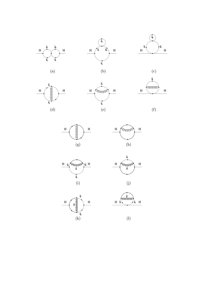
Figure 1: Feynman diagrams for the contribution of squark and quark loops to the Higgs-boson self-energies at the two-loop level ($H=\phi_{1},\phi_{2},A$).

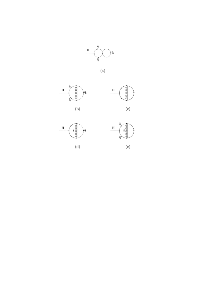
Figure 2: Feynman diagrams for the contributions of squark and quark loops to the Higgs-boson tadpoles at the two-loop level ($H=\phi_{1},\phi_{2}$).

Figure 3: One-loop counterterm contributions to the Higgs boson self-energies at the two-loop level ($H=\phi_{1},\phi_{2},A$).

Figure 4: One-loop counterterm contributions to the Higgs-boson tadpoles at the two-loop level ($H=\phi_{1},\phi_{2}$).

Figure 5: One-loop diagrams for the squark and quark mass counterterms and for the squark mixing-angle counterterm.

We now briefly describe the evaluation of the two-loop diagrams. As explained above, the calculation involves irreducible two-loop diagrams at zero momentum-transfer and counterterm diagrams. In deriving our results we have made strong use of computer algebra tools: the diagrams were generated with the Mathematica package FeynArts [20]. For this purpose we have implemented a model file which contains the relevant part of the MSSM Lagrangian, i.e. all SUSY propagators ($\tilde{t}_{1},\tilde{t}_{2},\tilde{b}_{1},\tilde{b}_{2},\tilde{g}$) needed for the QCD-corrections and the appropriate vertices (Higgs boson-squark vertices, squark-gluon and squark-gluino vertices). The program inserts propagators and vertices into the graphs in all possible ways and creates the amplitudes including all symmetry factors. The evaluation of the two-loop diagrams and counterterms was performed with the Mathematica package TwoCalc [21]. By means of two-loop tensor integral decompositions it reduces the amplitudes to a minimal set of standard scalar integrals, consisting in this case of products of the basic one-loop integrals $A_{0},B_{0}$ [22] (the $B_{0}$ functions originate from the counterterm contributions only) and the two-loop function $T_{134}$, which is the genuine two-loop scalar integral at zero momentum-transfer (vacuum integral). This integral is known for arbitrary internal masses and admits a compact representation for $\delta\to 0$ in terms of logarithms and dilogarithms (see for instance Ref. [23]). It should be noted that from the expansion of the one-loop two-point function $B_{0}$,

$$B_{0}(q^{2},m_{a},m_{b})=\frac{1}{\delta}+B_{0}^{\rm fin}(q^{2},m_{a},m_{b})+\delta\,B_{0}^{\delta}(q^{2},m_{a},m_{b}),$$ (114)

only the term $B_{0}^{\rm fin}$ contributes, while $B_{0}^{\delta}$ drops out in our final result. From the output generated with TwoCalc a FORTRAN code was created which allows a fast calculation for a given set of parameters. This code has been implemented into the FORTRAN program FeynHiggs [24], see below.

Our results for the two-loop $\phi_{1,2}$ self-energies are given in terms of the SUSY parameters $\tan\beta\hskip 2.84526pt$, $M_{A}$, $\mu$, $m_{\tilde{t}_{1}}$, $m_{\tilde{t}_{2}}$, $\theta_{\tilde{t}}$, and $m_{\tilde{g}}$. In the general case the results are by far too lengthy to be given here explicitly. In the special case of vanishing mixing in the $\tilde{t}$-sector, $\mu=0$, and $m_{\tilde{t}_{1}}=m_{\tilde{t}_{2}}=m_{\tilde{t}}$, a relatively compact expression can be derived which is given in Ref. [13]. We have performed an expansion of this result for large values of $m_{\tilde{g}}$. It yields for the leading terms

$$\hat{\Sigma}_{\phi_{2}}^{(2)}=C_{F}\frac{\alpha}{\pi}\frac{\alpha_{s}}{\pi}\frac{3\,m_{t}^{2}}{2\,s_{W}^{2}\sin^{2}\beta\hskip 2.84526pt}\left[-\ln^{2}(m_{\tilde{g}}^{2})+\ln(m_{\tilde{g}}^{2})\right]+{\cal O}(m_{\tilde{g}}^{0}).$$ (115)

This shows that the gluino does not decouple from the two-loop result, contrary to the case of the two-loop QCD contributions to the $\rho$-parameter in the MSSM [19, 25].

In Ref. [11] a result for the limiting case

$$m_{\tilde{t}}=m_{\tilde{t}_{1}}=m_{\tilde{t}_{2}}=m_{\tilde{g}}\gg m_{t},\qquad\tan\beta\hskip 2.84526pt\to\infty$$ (116)

has been given. In this limit we obtain

$$\hat{\Sigma}^{(2)}_{\phi_{1}}(0)=0,\;\;\;\;\hat{\Sigma}^{(2)}_{\phi_{1}\phi_{2}}(0)=0,$$

$$\hat{\Sigma}^{(2)}_{\phi_{2}}(0) = -C_{F}\frac{\alpha}{\pi}\frac{\alpha_{s}}{\pi}\frac{9\,m_{t}^{4}}{4s_{W}^{2}M_{W}^{2}}\ln\left(\frac{m_{\tilde{t}}^{2}}{m_{t}^{2}}\right)\left[\ln\left(\frac{m_{\tilde{t}}^{2}}{m_{t}^{2}}\right)+2\right],$$ (117)

which agrees with the corresponding result given in Ref. [11].

3.3 Determination of the Higgs-boson masses

In the Feynman-diagrammatic approach the Higgs-boson masses are derived beyond tree level by determining the poles of the $h-H$-propagator matrix whose inverse is given by

$$\left(\Delta_{\rm Higgs}\right)^{-1}=-i\left(\begin{array}[]{cc}q^{2}-m_{H,{\rm tree}}^{2}+\hat{\Sigma}_{H}(q^{2})&\hat{\Sigma}_{hH}(q^{2})\\ \hat{\Sigma}_{hH}(q^{2})&q^{2}-m_{h,{\rm tree}}^{2}+\hat{\Sigma}_{h}(q^{2})\end{array}\right),$$ (118)

where again the $\hat{\Sigma}$ denote the renormalized Higgs-boson self-energies, now in the $h-H$-basis.

Determining the poles of the matrix $\Delta_{\rm Higgs}$ in eq. (118) is equivalent to solving the equation

$$\left[q^{2}-m_{h}^{2}+\hat{\Sigma}_{hh}(q^{2})\right]\left[q^{2}-m_{H}^{2}+\hat{\Sigma}_{HH}(q^{2})\right]-\left[\hat{\Sigma}_{hH}(q^{2})\right]^{2}=0.$$ (119)

In our calculation the complete one-loop result for the Higgs-boson self-energies in the on-shell scheme [5] is combined with the leading two-loop contributions, which have been outlined in the previous section. The matrix eq. (118) therefore contains the renormalized Higgs-boson self-energies

$$\hat{\Sigma}_{s}(q^{2})=\hat{\Sigma}^{(1)}_{s}(q^{2})+\hat{\Sigma}^{(2)}_{s}(0),\quad s=h,H,hH,$$ (120)

where the momentum dependence is neglected only in the two-loop contribution.

Since the two-loop contribution has been calculated in the $\phi_{1}$-$\phi_{2}$-basis, a rotation into the $h$-$H$-basis, according to eq. (19), has to be performed:

$$\hat{\Sigma}^{(2)}_{H} = \cos^{2}\alpha\hskip 2.84526pt\hat{\Sigma}^{(2)}_{\phi_{1}}+\sin^{2}\alpha\hskip 2.84526pt\hat{\Sigma}^{(2)}_{\phi_{2}}+2\sin\alpha\hskip 2.84526pt\cos\alpha\hskip 2.84526pt\hat{\Sigma}^{(2)}_{\phi_{1}\phi_{2}}$$

$$\hat{\Sigma}^{(2)}_{h} = \sin^{2}\alpha\hskip 2.84526pt\hat{\Sigma}^{(2)}_{\phi_{1}}+\cos^{2}\alpha\hskip 2.84526pt\hat{\Sigma}^{(2)}_{\phi_{2}}-2\sin\alpha\hskip 2.84526pt\cos\alpha\hskip 2.84526pt\hat{\Sigma}^{(2)}_{\phi_{1}\phi_{2}}$$

$$\hat{\Sigma}^{(2)}_{hH} = -\sin\alpha\hskip 2.84526pt\cos\alpha\hskip 2.84526pt\left(\hat{\Sigma}^{(2)}_{\phi_{1}}-\hat{\Sigma}^{(2)}_{\phi_{2}}\right)+(\cos^{2}\alpha\hskip 2.84526pt-\sin^{2}\alpha\hskip 2.84526pt)\hat{\Sigma}^{(2)}_{\phi_{1}\phi_{2}}.$$ (121)

We have implemented two further corrections beyond ${\cal O}(\alpha\alpha_{s})$ into the prediction for $m_{h}$, which are illustrated in Figs. 6, 7, 9 and 10. The leading two-loop Yukawa correction of ${\cal O}(G_{F}^{2}m_{t}^{6})$ is taken over from the result obtained by renormalization group methods. It reads [8, 15]

$$\Delta m_{h}^{2} = \frac{9}{16\pi^{4}}G_{F}^{2}m_{t}^{6}\left[\tilde{X}t+t^{2}\right]$$ (122)

with $$\tilde{X}=\Bigg{[}\left(\frac{m_{\tilde{t}_{2}}^{2}-m_{\tilde{t}_{1}}^{2}}{4m_{t}^{2}}\sin^{2}2\theta_{\tilde{t}}\right)^{2}\left(2-\frac{m_{\tilde{t}_{2}}^{2}+m_{\tilde{t}_{1}}^{2}}{m_{\tilde{t}_{2}}^{2}-m_{\tilde{t}_{1}}^{2}}\log\left(\frac{m_{\tilde{t}_{2}}^{2}}{m_{\tilde{t}_{1}}^{2}}\right)\right)$$ (124)

$$\mbox{}\hskip 28.45274pt+\frac{m_{\tilde{t}_{2}}^{2}-m_{\tilde{t}_{1}}^{2}}{2m_{t}^{2}}\sin^{2}2\theta_{\tilde{t}}\log\left(\frac{m_{\tilde{t}_{2}}^{2}}{m_{\tilde{t}_{1}}^{2}}\right)\Bigg{]},$$

$$t=\frac{1}{2}\log\left(\frac{m_{\tilde{t}_{1}}^{2}m_{\tilde{t}_{2}}^{2}}{m_{t}^{4}}\right).$$

The second higher-order contribution which has been implemented concerns leading QCD corrections beyond two-loop order, taken into account by using the $\overline{\rm{MS}}$ top mass

$$\overline{m}_{t}=\overline{m}_{t}(m_{t})\approx\frac{m_{t}}{1+\frac{4}{3\,\pi}\alpha_{s}(m_{t})}$$ (125)

for the two-loop contributions instead of the pole mass, $m_{t}=175\,\,{\mathrm{G}eV}$. In the $\tilde{t}$ mass matrix, however, we continue to use the pole mass as an input parameter. Only when performing the comparison with the RG results we use $\overline{m}_{t}$ in the $\tilde{t}$ mass matrix for the two-loop result, since in the RG results the running masses appear everywhere. This three-loop effect gives rise to a shift up to $1.5\,\,{\mathrm{G}eV}$ in the prediction for $m_{h}$.

The complete one-loop calculation together with the leading two-loop corrections and the other corrections beyond ${\cal O}(\alpha\alpha_{s})$ have been implemented into the FORTRAN code FeynHiggs [24]. This code can be linked to existing programs as a subroutine, thus providing an accurate calculation of $m_{h}$ and $m_{H}$ which can be used for further phenomenological analyses. FeynHiggs is available via its WWW page
http://www-itp.physik.uni-karlsruhe.de/feynhiggs.

4 Numerical results for $m_{h}$ and $m_{H}$

4.1 Dependence of the results on the MSSM parameters

In this subsection we give a detailed discussion of the dependence of $m_{h}$ on the parameters of the MSSM. For $\tan\beta\hskip 2.84526pt$ we restrict ourselves to two typical values which are favored by SUSY-GUT scenarios [27]: $\tan\beta\hskip 2.84526pt=1.6$ for the $SU(5)$ scenario and $\tan\beta\hskip 2.84526pt=40$ for the $SO(10)$ scenario. Other parameters are $M_{Z}=91.187\,\,{\mathrm{G}eV},M_{W}=80.375\,\,{\mathrm{G}eV},G_{F}=1.16639\,10^{-5}\,\,{\mathrm{G}eV}^{-2},\alpha_{s}(m_{t})=0.1095$, $m_{t}=175\,\,{\mathrm{G}eV}$, and $m_{b}=4.5\,\,{\mathrm{G}eV}$ (if not indicated differently). The parameter $M$ appearing in the plots is the $SU(2)$ gaugino mass parameter. The other gaugino mass parameter, $M_{1}$, is fixed via the GUT relation

$$M_{1}=\frac{5}{3}\frac{s_{W}^{2}}{c_{W}^{2}}M~{}.$$ (126)

The scalar top masses and the mixing angle are related to the parameters $M_{{\tilde{t}}_{L}}$, $M_{{\tilde{t}}_{R}}$ and $M_{t}^{LR}$ of the $\tilde{t}$ mass matrix, which reads

$${\cal M}^{2}_{\tilde{t}}=\left(\begin{array}[]{cc}M_{\tilde{t}_{L}}^{2}+m_{t}^{2}+\cos 2\beta\hskip 2.84526pt(\frac{1}{2}-\frac{2}{3}s_{W}^{2})M_{Z}^{2}&m_{t}M_{t}^{LR}\\ m_{t}M_{t}^{LR}&M_{\tilde{t}_{R}}^{2}+m_{t}^{2}+\frac{2}{3}\cos 2\beta\hskip 2.84526pts_{W}^{2}M_{Z}^{2}\end{array}\right)~{},$$ (127)

with

$$M_{t}^{LR}=A_{t}-\mu\cot\beta\hskip 2.84526pt~{}.$$ (128)

In the figures below we have chosen $m_{\tilde{q}}\equiv M_{\tilde{t}_{L}}=M_{\tilde{t}_{R}}$ (if not indicated differently).

Fig. 6 shows the result for $m_{h}$ obtained from the diagrammatic calculation of the full one-loop and leading two-loop contributions. The two contributions beyond ${\cal O}(\alpha\alpha_{s})$ discussed above are shown in separate curves. For comparison the pure one-loop result is also given. The results are plotted as a function of $M_{t}^{LR}/m_{\tilde{q}}$, where $m_{\tilde{q}}$ is fixed to $500\,\,{\mathrm{G}eV}$. The two-loop contributions give rise to a large reduction of the one-loop result of 10–20 GeV. The two corrections beyond ${\cal O}(\alpha\alpha_{s})$ both increase $m_{h}$ by up to $2\,\,{\mathrm{G}eV}$. A minimum occurs around $M_{t}^{LR}=0\,\,{\mathrm{G}eV}$ which we refer to as ‘no mixing’. A maximum in the two-loop result for $m_{h}$ is reached for about $M_{t}^{LR}/m_{\tilde{q}}\approx\pm 2$ in the $\tan\beta\hskip 2.84526pt=1.6$ scenario as well as in the $\tan\beta\hskip 2.84526pt=40$ scenario. This case we refer to as ‘maximal mixing’. The position of the maximum is shifted compared to its one-loop value of about $M_{t}^{LR}/m_{\tilde{q}}\approx\pm 2.4$. The Yukawa correction and the insertion of the running top mass have only a negligible effect on the location of the maximum.

Figure 6: One- and two-loop results for $m_{h}$ as a function of $M_{t}^{LR}/m_{\tilde{q}}$ for two values of $\tan\beta\hskip 2.84526pt$. The corrections beyond ${\cal O}(\alpha\alpha_{s})$ discussed in the text are shown separately.

Figure 7: One- and two-loop results for $m_{H}$ as a function of $M_{t}^{LR}/m_{\tilde{q}}$ for two values of $\tan\beta\hskip 2.84526pt$. The running top mass correction discussed in the text is shown separately.

Fig. 7 depicts the result for the heavy Higgs-boson mass, $m_{H}$, obtained in the same way as $m_{h}$ above. The only difference is that no Yukawa term has been included. In the plot we have chosen the small value $M_{A}=75\,\,{\mathrm{G}eV}$, close to the lower experimental bound, since only for a light $A$ boson the higher-order corrections give a sizable contribution (see also Fig. 8). Here the values for $m_{H}$ obtained for small $\tan\beta\hskip 2.84526pt$ are larger than for $\tan\beta\hskip 2.84526pt=40$. The values of $M_{t}^{LR}/m_{\tilde{q}}$ for which $m_{H}$ is maximal depend in this case on $\tan\beta\hskip 2.84526pt$ and the sign of $M_{t}^{LR}$.

                       

Figure 8: $m_{h}$ and $m_{H}$ are shown as a function of $M_{A}$ for $\tan\beta\hskip 2.84526pt=1.6$ and $\tan\beta\hskip 2.84526pt=40$. The two-loop value for $m_{h}$ contains both corrections beyond ${\cal O}(\alpha\alpha_{s})$, whereas for $m_{H}$ only the running top mass effect is included. The maximal-mixing scenario corresponds to the definition according to the discussion of Fig. 6.

Both Higgs-boson masses are shown in Fig. 8 for low and high $\tan\beta\hskip 2.84526pt$ and the no-mixing and the maximal-mixing case, where the latter case corresponds to the definition according to Fig. 6 for the light Higgs boson. For $m_{H}$ sizable corrections at the one- and two-loop level are obtained only for $M_{A}\;\raisebox{-3.00003pt}{$\stackrel{{\scriptstyle\displaystyle<}}{{\sim}}$}\;200\,\,{\mathrm{G}eV}$ for $\tan\beta\hskip 2.84526pt=1.6$ and for $M_{A}\;\raisebox{-3.00003pt}{$\stackrel{{\scriptstyle\displaystyle<}}{{\sim}}$}\;120\,\,{\mathrm{G}eV}$ for $\tan\beta\hskip 2.84526pt=40$.

More relevant for todays’ colliders is the mass of the lighter Higgs boson, $m_{h}$, on which we will focus in the following discussion. In Fig. 9 $m_{h}$ is shown in the two scenarios with $\tan\beta\hskip 2.84526pt=1.6$ and $\tan\beta\hskip 2.84526pt=40$ as a function of $m_{\tilde{q}}$ for no mixing and maximal mixing and for $M_{A}=200,1000\,\,{\mathrm{G}eV}$. The tree-level, the one-loop and the two-loop results with the two corrections beyond ${\cal O}(\alpha\alpha_{s})$ are shown (the values of $m_{\tilde{q}}$ are such that the corresponding $\tilde{t}$-masses lie within the experimentally allowed region). In all scenarios of Fig. 9 the two-loop corrections give rise to a large reduction of the one-loop value of $m_{h}$. The effect is generally larger in the $\tan\beta\hskip 2.84526pt=1.6$ scenario, and for maximal mixing and large $M_{A}$. The inclusion of the Yukawa correction and the running top mass leads to a slight shift in $m_{h}$ towards higher values. This effect amounts up to $20\%$ of the two-loop correction. In the $\tan\beta\hskip 2.84526pt=1.6$ scenario with $m_{\tilde{q}}=1\,\,{\mathrm{T}eV}$, $m_{h}$ reaches about $75~{}(81)\,\,{\mathrm{G}eV}$ for $M_{A}=200~{}(1000)\,\,{\mathrm{G}eV}$ in the no-mixing case, and $94~{}(101)\,\,{\mathrm{G}eV}$ in the maximal-mixing case. For $\tan\beta\hskip 2.84526pt=40$ the respective values of $m_{h}$ are $112\,\,{\mathrm{G}eV}$ in the no-mixing case, and $126\,\,{\mathrm{G}eV}$ in the maximal-mixing case for both values of $M_{A}$. The peaks in the plots for $M_{A}=1\,\,{\mathrm{T}eV}$ are due to the threshold $M_{A}=m_{\tilde{b}_{1}}+m_{\tilde{b}_{2}}$ in the one-loop contribution, originating from the sbottom-loop diagram in the $A$ self-energy.

                       

                       

Figure 9: The mass of the lightest Higgs boson for $\tan\beta\hskip 2.84526pt=1.6$ and $\tan\beta\hskip 2.84526pt=40$. The tree-level, the one-loop and the two-loop results for $m_{h}$ are shown as a function of $m_{\tilde{q}}$ for the no-mixing and the maximal-mixing case, and for $M_{A}=200,1000\,\,{\mathrm{G}eV}$.

The dependence of $m_{h}$ on $M_{A}$ is depicted in Fig. 10 in the two scenarios with $\tan\beta\hskip 2.84526pt=1.6$ and $\tan\beta\hskip 2.84526pt=40$ for no mixing and maximal mixing for $m_{\tilde{q}}=500,1000\,\,{\mathrm{G}eV}$. In all scenarios of Fig. 10 the two-loop corrections give rise to a large reduction of the one-loop value of $m_{h}$. A saturation effect can be observed for $M_{A}\;\raisebox{-3.00003pt}{$\stackrel{{\scriptstyle\displaystyle>}}{{\sim}}$}\;300~{}(150)\,\,{\mathrm{G}eV}$ in the $\tan\beta\hskip 2.84526pt=1.6~{}(40)$ scenario. The peaks in the plots for $M_{A}=350\,\,{\mathrm{G}eV}$ are due to the threshold $M_{A}=2\,m_{t}$ in the one-loop contribution, originating from the top-loop diagram in the $A$ self-energy.

                       

                       

Figure 10: The mass of the lightest Higgs boson as a function of $M_{A}$ for $\tan\beta\hskip 2.84526pt=1.6$ and $\tan\beta\hskip 2.84526pt=40$. The tree-level, the one-loop and the two-loop results for $m_{h}$ are shown in the no-mixing and the maximal-mixing case, and for $m_{\tilde{q}}=500,1000\,\,{\mathrm{G}eV}$.

Allowing for a splitting between the parameters $M_{\tilde{t}_{L}}$, $M_{\tilde{t}_{R}}$ in the $\tilde{t}$ mass matrix yields maximal values of $m_{h}$ which are approximately the same as for the case $m_{\tilde{q}}=M_{\tilde{t}_{L}}=M_{\tilde{t}_{R}}$, provided that one sets

$$m_{\tilde{q}_{\bigr{|}M_{\tilde{t}_{L}}=M_{\tilde{t}_{R}}}}={\rm max}\{M_{\tilde{t}_{L}},M_{\tilde{t}_{R}}\}_{\Bigr{|}M_{\tilde{t}_{L}}\neq M_{\tilde{t}_{R}}}~{},$$ (129)

see Fig. 11. However, the location of the maximal Higgs-boson mass, depending on $M_{t}^{LR}$, is shifted towards smaller values, typically by about 40%. The numerical difference in $m_{h}$ in the two splitting scenarios $M_{\tilde{t}_{L}}/M_{\tilde{t}_{R}}=300/1000$ and $M_{\tilde{t}_{L}}/M_{\tilde{t}_{R}}=1000/300$ is small. They differ by up to $2\,\,{\mathrm{G}eV}$ only in the large $\tan\beta\hskip 2.84526pt$ scenario when $M_{t}^{LR}>1000\,\,{\mathrm{G}eV}$.

                       

                       

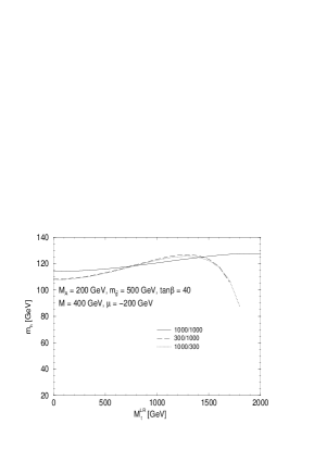
Figure 11: The mass of the lightest Higgs boson as a function of $M_{t}^{LR}$ for differently split values of the soft SUSY breaking terms. The curves in the plots correspond to the values $M_{\tilde{t}_{L}}/M_{\tilde{t}_{R}}=1000/1000,~{}300/1000$ and $1000/300$.

The variation of $m_{h}$ with $m_{t}$ is rather strong. The scenarios for no mixing and maximal mixing and for $\tan\beta\hskip 2.84526pt=1.6$ and $\tan\beta\hskip 2.84526pt=40$ are shown in Fig. 12, where $m_{t}$ is varied around the central value of $m_{t}=175\,\,{\mathrm{G}eV}$ by $\pm 10\,\,{\mathrm{G}eV}$. The variation of $m_{h}$ is stronger for low $\tan\beta\hskip 2.84526pt$ and larger $m_{\tilde{q}}$: in the $\tan\beta\hskip 2.84526pt=1.6$ scenario $m_{h}$ varies by more than $10\,\,{\mathrm{G}eV}$ and about $20\,\,{\mathrm{G}eV}$ for no-mixing and maximal-mixing, respectively. In the $\tan\beta\hskip 2.84526pt=40$ scenario the respective values are less than $10\,\,{\mathrm{G}eV}$ and about $15\,\,{\mathrm{G}eV}$.

                       

                       

Figure 12: The mass of the lightest Higgs boson is shown as a function of $m_{t}$: the scenarios of no mixing and maximal mixing are depicted for low and high $\tan\beta\hskip 2.84526pt$, and $\mu=-200\,\,{\mathrm{G}eV},M=400\,\,{\mathrm{G}eV}$.

Varying $\tan\beta\hskip 2.84526pt$ around the value $\tan\beta\hskip 2.84526pt=1.6$ has a relatively large impact on $m_{h}$ (higher values for $m_{h}$ are obtained for larger $\tan\beta\hskip 2.84526pt$), while the effect of varying $\tan\beta\hskip 2.84526pt$ around $\tan\beta\hskip 2.84526pt=40$ is marginal. This is shown in Fig. 13 for $M_{A}=200,1000\,\,{\mathrm{G}eV}$, $m_{\tilde{q}}=200,1000\,\,{\mathrm{G}eV}$ for the no-mixing and the maximal-mixing scenario. For $\tan\beta\hskip 2.84526pt>15$ the variation is less than $1\,\,{\mathrm{G}eV}$.

                       

                       

Figure 13: The mass of the lightest Higgs boson is shown as a function of $\tan\beta\hskip 2.84526pt$. $m_{h}$ is plotted for the scenarios with $M_{A}=200,500\,\,{\mathrm{G}eV}$ and $m_{\tilde{q}}=500,1000\,\,{\mathrm{G}eV}$ in the no-mixing and the maximal-mixing case.

In Fig. 14 $m_{h}$ is shown as a function of $M$, the soft SUSY breaking parameter in the chargino and neutralino sector (see Sec. 126). In our calculation $M$ enters only in the one-loop self-energies. The variation is less than $4\,\,{\mathrm{G}eV}$ for the whole $M$ parameter space. For increasing $M$ the result for $m_{h}$ decreases in general.

The dependence of $m_{h}$ on $\mu$, the Higgs mixing parameter, is depicted in Fig. 15. The parameter $\mu$ enters via the non-diagonal Higgs-squark coupling at one- and two-loop order and via the chargino and neutralino sector in the one-loop self-energies. It should be noted that for the plots in Fig. 15 we have set $m_{b}=0\,\,{\mathrm{G}eV}$, thus suppressing the contribution of the $b-\tilde{b}$-sector. The reason is that for large $\mu$ and for large $\tan\beta\hskip 2.84526pt$ some Higgs-sbottom couplings can become rather large, which makes the perturbative calculation questionable in this case. The variation of $m_{h}$ with $\mu$ in Fig. 15 is relatively weak, not exceeding $3\,\,{\mathrm{G}eV}$. A maximum (for the choice $M=400\,\,{\mathrm{G}eV}$) for $m_{h}$ lies between $\mu=-200\,\,{\mathrm{G}eV}$ and $\mu=-100\,\,{\mathrm{G}eV}$. For decreasing $M$ the maximum is reached for slightly smaller values of $\mu$, see also Sec. 4.2.

                       

Figure 14: The mass of the lightest Higgs boson is shown as a function of $M$, the soft SUSY breaking parameter of the chargino and neutralino sector.

                       

Figure 15: The mass of the lightest Higgs boson is shown as a function of $\mu$, the Higgs mixing parameter. The mass of the bottom quark, $m_{b}$, is set to zero in order to avoid unnaturally large one-loop effects.

Finally we show the dependence on the gluino mass, $m_{\tilde{g}}$, which enters only at the two-loop level. Fig. 16 depicts $m_{h}$ as a function of $m_{\tilde{g}}$ in the scenarios with $m_{\tilde{q}}=500,1000\,\,{\mathrm{G}eV}$ for $\tan\beta\hskip 2.84526pt=1.6$ and $\tan\beta\hskip 2.84526pt=40$ in the no-mixing and the maximal-mixing case. Small variations below $1\,\,{\mathrm{G}eV}$ occur in the no-mixing scenario, while change in $m_{h}$ up to $4\,\,{\mathrm{G}eV}$ arises in the maximal-mixing scenario. $m_{h}$ reaches a maximum at about $m_{\tilde{g}}\approx 0.8\,m_{\tilde{q}}$. Since the parameter $m_{\tilde{g}}$ is absent in the RG approach, a variation of $m_{h}$ with $m_{\tilde{g}}$ can directly be seen as a deviation of the diagrammatic result from the RG result, see Sec. 4.3.

                       

                       

Figure 16: The mass of the lightest Higgs boson as a function of $m_{\tilde{g}}$ for a common value of $M_{A}=500\,\,{\mathrm{G}eV},m_{\tilde{q}}=500,1000\,\,{\mathrm{G}eV}$ for the no-mixing and the maximal-mixing case and for low and high $\tan\beta\hskip 2.84526pt$.

As pointed out in Ref. [14] it is desirable to express the predictions for the observable $m_{h}$ in terms of other physical observables. This provides the possibility to directly compare results obtained by different approaches making use of different renormalization schemes. Therefore we show in Fig. 17 the dependence of $m_{h}$ on the parameters $m_{\tilde{t}_{1}},m_{\tilde{t}_{2}}$ and $\theta_{\tilde{t}}$, which, since we are working in the on-shell scheme, directly correspond to the physical ones. We show $m_{h}$ as a function of $m_{\tilde{t}_{2}}$ for $\Delta m_{\tilde{t}}=0\,\,{\mathrm{G}eV}$ and $\theta_{\tilde{t}}=0$ (no mixing) and for $\Delta m_{\tilde{t}}=340\,\,{\mathrm{G}eV}$ and $\theta_{\tilde{t}}=-\pi/4$ (maximal mixing), where $\Delta m_{\tilde{t}}\equiv m_{\tilde{t}_{2}}-m_{\tilde{t}_{1}}$. The choice of $\Delta m_{\tilde{t}}\approx 340\,\,{\mathrm{G}eV}$ corresponds to $M_{t}^{LR}/m_{\tilde{q}}\approx 2$ in terms of the soft SUSY breaking parameters. The two-loop results shown here contain also the corrections beyond ${\cal O}(\alpha\alpha_{s})$. In these plots we have furthermore imposed the $\rho\,$-parameter constraint: We have required that the contribution of the third generation of scalar quarks to the $\rho$-parameter [19, 25] does not exceed the value of $1.3\cdot 10^{-3}$, which corresponds approximately to the resolution of $\Delta\rho$ when it is determined from experimental data [28]. For $\tan\beta\hskip 2.84526pt=1.6$ $m_{h}$ reaches about $76~{}(82)\,\,{\mathrm{G}eV}$ for $M_{A}=200~{}(1000)\,\,{\mathrm{G}eV},m_{\tilde{t}_{2}}=1\,\,{\mathrm{T}eV}$ and no mixing in the $\tilde{t}$-sector. In the maximal-mixing case the reached values of $m_{h}$ are $94~{}(101)\,\,{\mathrm{G}eV}$. In the $\tan\beta\hskip 2.84526pt=40$ scenario, $m_{h}$ reaches $114~{}(127)\,\,{\mathrm{G}eV}$ in the no-mixing (maximal-mixing) case for both values of $M_{A}$. The peaks in the plots for $M_{A}=1\,\,{\mathrm{T}eV}$ and maximal mixing in the $\tilde{t}$-sector around $m_{\tilde{t}_{2}}=660\,\,{\mathrm{G}eV}$ are due to the threshold $M_{A}=m_{\tilde{t}_{1}}+m_{\tilde{t}_{2}}$ in the one-loop contribution, originating from the stop-loop diagram in the $A$ self-energy.

                       

                       

Figure 17: The mass of the lightest Higgs boson in terms of the physical parameters $m_{\tilde{t}_{1}},m_{\tilde{t}_{2}}$ and $\theta_{\tilde{t}}$, where $\Delta m_{\tilde{t}}\equiv m_{\tilde{t}_{2}}-m_{\tilde{t}_{1}}$. The scenarios $\Delta m_{\tilde{t}}=0\,\,{\mathrm{G}eV},\theta_{\tilde{t}}=0$ (no mixing) and $\Delta m_{\tilde{t}}=340\,\,{\mathrm{G}eV},\theta_{\tilde{t}}=-\pi/4$ (maximal mixing) are shown.

4.2 Upper bound for $m_{h}$ as a function of $\tan\beta\hskip 2.84526pt$

Since, as shown in Fig. 13, smaller values for $m_{h}$ are obtained for small $\tan\beta\hskip 2.84526pt$, this part of the parameter space can to a large extend be covered at todays’ colliders. The discovery limit for $m_{h}$ at LEP2 is expected to be slightly above $100\,\,{\mathrm{G}eV}$ [29]. In this context it is of special interest to know the maximally possible value for $m_{h}$ as a function of $\tan\beta\hskip 2.84526pt$ in the MSSM. To this end we have performed a parameter scan, varying $m_{\tilde{g}},M,\mu,M_{A}$ and $M_{t}^{LR}$ for three values of $m_{t}$ and fixed values of $m_{\tilde{q}}$ and $\tan\beta\hskip 2.84526pt$. The maximal values for $m_{h}$, including also the Yukawa correction and the contribution from the running top mass, were reached (in the case $m_{t}=175\,\,{\mathrm{G}eV}$) for

$$m_{\tilde{g}} \approx 0.8\,m_{\tilde{q}}$$

$$M \approx 0\,\,{\mathrm{G}eV}$$

$$\mu \approx 0\,\,{\mathrm{G}eV}$$

$$M_{A} \approx \left\{\begin{array}[]{l}800\,\,{\mathrm{G}eV}\;\mbox{for small}\tan\beta\\ 360\,\,{\mathrm{G}eV}\;\mbox{for large}\tan\beta\end{array}\right.$$ (131)

$$M_{t}^{LR} \approx 2\,m_{\tilde{q}}$$ (132)

in all scenarios.

The value for $M_{A}$ in (132) needs some further explanation: as one can see in Fig. 10, due to a one-loop threshold effect the value of $m_{h}$ can become very large for $M_{A}=2\,m_{t}$. For large $\tan\beta\hskip 2.84526pt$ this threshold effect results in a bigger $m_{h}$ value for $M_{A}$ in the region around $2\,m_{t}$ than for larger values of $M_{A}$ (with $M_{A}<1500\,\,{\mathrm{G}eV}$, where we stopped our scan.) Of course the exact value $M_{A}=2\,m_{t}=2\cdot 175\,\,{\mathrm{G}eV}=350\,\,{\mathrm{G}eV}$ would be a very specific choice, giving a wrong impression of the possible size of $m_{h}$. (Exactly at the threshold also finite width effects for the $A$ boson would have to be taken into account.) Therefore we have chosen the value $M_{A}=360\,\,{\mathrm{G}eV}$ which is not directly at the threshold, thus giving a more realistic impression about the maximally possible values for $m_{h}$. The choice $M=\mu=0\,\,{\mathrm{G}eV}$ is experimentally excluded. We nevertheless use these values since the difference in $m_{h}$ to the case with experimentally not excluded $M$ and $\mu$ is very small, typically below $0.5\,\,{\mathrm{G}eV}$.

In Fig. 18 we show the maximal Higgs-boson mass value, including also the corrections beyond ${\cal O}(\alpha\alpha_{s})$, as a function of $\tan\beta\hskip 2.84526pt$; the other parameters are chosen according to eqs. (132). For the top-quark mass the most recent experimental value $m_{t}=173.8\,\,{\mathrm{G}eV}$ [30] is chosen and, since $m_{h}$ grows with increasing $m_{t}$, the experimental value plus one and plus two standard deviations ($m_{t}=178.8,183.8\,\,{\mathrm{G}eV}$). The common squark mass parameter is chosen to be $m_{\tilde{q}}=1000\,\,{\mathrm{G}eV}$ as a high, and $m_{\tilde{q}}=2000\,\,{\mathrm{G}eV}$ as a very high value. On the left side of Fig. 18 we show the full $\tan\beta\hskip 2.84526pt$ range ($\tan\beta\hskip 2.84526pt\leq 50$), whereas on the right side we focus on the range especially interesting for LEP2 and the upgraded Tevatron ($\tan\beta\hskip 2.84526pt\leq 5$).

In the $\tan\beta\hskip 2.84526pt\leq 5$ plot we have chosen $M_{A}=800\,\,{\mathrm{G}eV}$. In the $\tan\beta\hskip 2.84526pt\leq 50$ plot, however, we have chosen $M_{A}=800\,\,{\mathrm{G}eV}$ only for $\tan\beta\hskip 2.84526pt\leq 4$; for larger values we have switched to $M_{A}=360\,\,{\mathrm{G}eV}$. For the value $\tan\beta\hskip 2.84526pt=4$ one gets about the same maximal value for $m_{h}$ for both choices of $M_{A}$.

	$\tan\beta\hskip 2.84526pt=1.6$		$\tan\beta\hskip 2.84526pt=1.7$		$\tan\beta\hskip 2.84526pt=1.8$		$\tan\beta\hskip 2.84526pt=1.9$		$\tan\beta\hskip 2.84526pt=2.0$
	$m_{\tilde{q}}$ =		$m_{\tilde{q}}$ =		$m_{\tilde{q}}$ =		$m_{\tilde{q}}$ =		$m_{\tilde{q}}$ =
$m_{t}$	1000	2000	1000	2000	1000	2000	1000	2000	1000	2000
173.8	103.0	106.1	104.4	107.4	105.8	108.8	107.2	110.1	108.5	111.3
178.8	108.1	111.6	109.4	112.9	110.8	114.2	112.1	115.4	113.3	116.6
183.8	113.4	117.4	114.7	118.6	116.0	119.8	117.2	120.9	118.4	122.0

Table 1: Maximal values for $m_{h}$ for different choices of $m_{t},m_{\tilde{q}}$ and $\tan\beta\hskip 2.84526pt$. All other parameters have been chosen according to eqs. (132). (All masses are in GeV.)

In the interesting region around $\tan\beta\hskip 2.84526pt=1.6$ the covered region of the $\tan\beta\hskip 2.84526pt$-parameter space depends strongly on the maximally accessible energy of todays’ colliders, see Tab. 1. For an exclusion limit of $m_{h}>107\,\,{\mathrm{G}eV}$, for instance, LEP2 covers $\tan\beta\hskip 2.84526pt<1.6$ completely only if $m_{t}$ is constrained to its present $1\,\sigma$ limit. On the other hand, taking a very conservative point of view and choosing $m_{t}$ at the $2\,\sigma$ bound, no limit on $\tan\beta\hskip 2.84526pt$ can be set, even for $m_{\tilde{q}}=1000\,\,{\mathrm{G}eV}$.

One should keep in mind, however, that the Higgs-boson masses depicted in Fig. 18 are the maximally possible upper values, i.e. for smaller mixing in the $\tilde{t}$-sector the region $\tan\beta\hskip 2.84526pt<1.6$ can be covered by LEP2 for all other sets of parameters. One can also see that a precise measurement of $m_{t}$ is decisive in order to set stringent bounds on $\tan\beta\hskip 2.84526pt$ in the MSSM.

In conclusion, our results confirm that for the scenario with $\tan\beta\hskip 2.84526pt=1.6$ the parameter space of the MSSM can be covered to a very large extent. Only for maximal mixing, very large soft SUSY breaking parameters in the $\tilde{t}$-sector and $m_{t}$ at its upper $(1-2)\sigma$ limit the light Higgs boson can escape the detection at LEP2. For increasing $\tan\beta\hskip 2.84526pt$, however, the parameter space in which the Higgs boson is not accessible at LEP2 increases rapidly.

Concerning the large $\tan\beta\hskip 2.84526pt$ region, LEP2 and the upgraded Tevatron can probe only the region of no mixing in the $\tilde{t}$-sector. The LHC and a future linear $e^{+}e^{-}$-collider are needed in order to test the parameter space with large $\tilde{t}$-mixing.

                       

                       

Figure 18: The maximally possible value for $m_{h}$, including all refinement terms, as a function of $\tan\beta\hskip 2.84526pt$, depending on the unphysical parameters $m_{\tilde{q}}$ and $M_{t}^{LR}$. The other MSSM parameters have been chosen according to eqs. (132).

In an analogous way we have also analyzed the maximal value for $m_{h}$ as a function of the physical parameters, see Fig. 19 and Tab. 2. We have chosen $m_{\tilde{t}_{2}}=1000,2000\,\,{\mathrm{G}eV}$, $\Delta m_{\tilde{t}}=340\,\,{\mathrm{G}eV}$ and $\theta_{\tilde{t}}=-\pi/4$. The other MSSM parameters are chosen according to eqs. (132). Fig. 19 shows the result for the maximal range of $\tan\beta\hskip 2.84526pt$ and for the interesting range for LEP2, $\tan\beta\hskip 2.84526pt\leq 5$. The results in Fig. 19 and Tab. 2 are slightly lower than the values obtained with the unphysical input parameters. This is due to the fact that the values obtained for the squark masses in the first scenario (for all other parameters chosen to be equal) are always larger than for the latter case with physical input parameters. The analysis of the upper bound of $m_{h}$, however, can be taken over directly from the case with unphysical input parameters.

	$\tan\beta\hskip 2.84526pt=1.6$		$\tan\beta\hskip 2.84526pt=1.7$		$\tan\beta\hskip 2.84526pt=1.8$		$\tan\beta\hskip 2.84526pt=1.9$		$\tan\beta\hskip 2.84526pt=2.0$
	$m_{\tilde{t}_{2}}$ =		$m_{\tilde{t}_{2}}$ =		$m_{\tilde{t}_{2}}$ =		$m_{\tilde{t}_{2}}$ =		$m_{\tilde{t}_{2}}$ =
$m_{t}$	1000	2000	1000	2000	1000	2000	1000	2000	1000	2000
173.8	101.8	105.9	103.3	107.2	104.7	108.6	106.1	109.9	107.5	111.2
178.8	106.6	111.3	108.0	112.6	109.4	113.9	110.8	115.2	112.1	116.4
183.8	111.5	116.9	112.9	118.1	114.2	119.4	115.5	120.6	116.7	121.7

Table 2: Maximal values for $m_{h}$ for different choices of $m_{t},m_{\tilde{t}_{2}}$ and $\tan\beta\hskip 2.84526pt$. All other parameters have been chosen according to eqs. (132). (All masses are in GeV.)

                       

                       

Figure 19: The maximally possible value for $m_{h}$, including all refinement terms, as a function of $\tan\beta\hskip 2.84526pt$, depending on the physical parameters $m_{\tilde{t}_{2}},\Delta m_{\tilde{t}}$ and $\theta_{\tilde{t}}$. The other MSSM parameters have been chosen according to eqs. (132).

4.3 Numerical comparison with the RG approach

We now turn to the comparison of our diagrammatic results with the predictions obtained via RG methods. For this comparison we made use of the FORTRAN code corresponding to Ref. [9], except for the one-loop results in Figs. 20 and 21, where we used the code described in Ref. [10].

We begin with the case of large values of $M_{A}$, for which the RG approach is most easily applicable and is expected to work most accurately. In order to study different contributions separately, we have first compared the diagrammatic one-loop on-shell result [5] with the one-loop leading log result (without renormalization group improvement) given in Ref. [10]. Since the available code uses the running top mass $\overline{m}_{t}=\overline{m}_{t}(m_{t})\approx 167.3\,\,{\mathrm{G}eV}$ we have also used this top mass for the full diagrammatic one-loop calculation. In Fig. 20 the lightest Higgs-boson mass is shown in the no-mixing scenario, i.e. $M_{t}^{LR}=0\,\,{\mathrm{G}eV}$, whereas in Fig. 21 $m_{h}$ is shown for increasing mixing in the $\tilde{t}$-sector. We found very good agreement, typically within $1\,\,{\mathrm{G}eV}$ for both mixing cases and low and high $\tan\beta\hskip 2.84526pt$. Only for very small values of $m_{\tilde{q}}$ a deviation up to $2\,\,{\mathrm{G}eV}$ arises. For values of $M_{A}$ below $100\,\,{\mathrm{G}eV}$ (which are not shown here) and large mixing in the $\tilde{t}$-sector deviations of about $5\,\,{\mathrm{G}eV}$ occur.

                       

Figure 20: Comparison between the one-loop Feynman-diagrammatic calculations and the results obtained by renormalization group methods [10]. The mass of the lightest Higgs boson is shown for the two scenarios with $\tan\beta\hskip 2.84526pt=1.6$ and $\tan\beta\hskip 2.84526pt=40$ as a function of $M_{t}^{LR}/m_{\tilde{q}}$ for $M_{A}=200,1000\,\,{\mathrm{G}eV}$.

Figure 21: Comparison between the one-loop Feynman-diagrammatic calculations and the results obtained by renormalization group methods [10]. The mass of the lightest Higgs boson is shown for the two scenarios with $\tan\beta\hskip 2.84526pt=1.6$ and $\tan\beta\hskip 2.84526pt=40$ as a function of $M_{t}^{LR}/m_{\tilde{q}}$ for $M_{A}=200,1000\,\,{\mathrm{G}eV}$.

In the next step of comparison we analyzed the no-mixing case at the two-loop level: we have compared our diagrammatic result for the no-mixing case, including the Yukawa correction and the running top mass effect, with the RG results obtained in Ref. [9]. We have adopted the scale $M$ (the $SU(2)$ gaugino mass parameter) as $M=m_{\tilde{q}}$, in order to treat it in the same way as it has been done in the RG approach. As can be seen in Fig. 22, after the inclusion of the corrections beyond ${\cal O}(\alpha\alpha_{s})$ the diagrammatic result for the no-mixing case agrees very well with the RG result. For the scenario with $M_{A}=1000\,\,{\mathrm{G}eV}$ the deviation between the results exceeds $2\,\,{\mathrm{G}eV}$ only for $\tan\beta\hskip 2.84526pt=1.6$ and $m_{\tilde{q}}<150\,\,{\mathrm{G}eV}$. For $M_{A}=200\,\,{\mathrm{G}eV}$ the deviation is in general slightly larger than for $M_{A}=1000\,\,{\mathrm{G}eV}$, but does not exceed $2\,\,{\mathrm{G}eV}$.

                       

                       

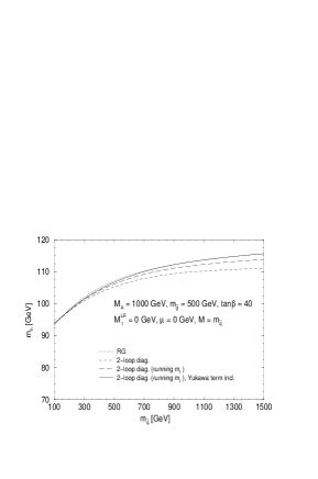
Figure 22: Comparison between the Feynman-diagrammatic calculations and the results obtained by renormalization group methods [9]. The mass of the lightest Higgs boson is shown for the scenarios with $\tan\beta\hskip 2.84526pt=1.6$ and $\tan\beta\hskip 2.84526pt=40$, $M_{A}=200,1000\,\,{\mathrm{G}eV}$ for the case of vanishing mixing in the $\tilde{t}$-sector.

The RG results do not contain the gluino mass as a parameter. Hence, varying $m_{\tilde{g}}$, which has been discussed in Sec. 4.1, gives rise to an extra deviation. In the no-mixing case this extra deviation does not exceed $1\,\,{\mathrm{G}eV}$. Varying the other parameters $\mu$ and $M$ in general does not lead to a sizable effect in the comparison with the corresponding RG results (as long as $M_{t}^{LR}$ is taken as input and a variation of $\mu$ does not affect the $\tilde{t}$-mixing.)

Finally we consider the situation where mixing in the $\tilde{t}$ sector is taken into account. In Fig. 23 our diagrammatic result, including the Yukawa correction and the running top mass effect, is compared with the RG results [9] as a function of $M_{t}^{LR}/m_{\tilde{q}}$ for the cases $\tan\beta\hskip 2.84526pt=1.6$ and $\tan\beta\hskip 2.84526pt=40$, and for $m_{\tilde{q}}=500,1000\,\,{\mathrm{G}eV}$ and $M_{A}=200\,\,{\mathrm{G}eV}$. The $M_{A}=1000\,\,{\mathrm{G}eV}$ scenario is depicted in Fig. 24 for the same set of parameters. The point $M_{t}^{LR}/m_{\tilde{q}}=0$ corresponds to the plots shown in Fig. 22, except that the parameter $\mu$ is set to $\mu=-m_{\tilde{q}}$ here. For larger $\tilde{t}$-mixing, sizable deviations between the diagrammatic and the RG results occur. They can reach $5\,\,{\mathrm{G}eV}$ for moderate mixing and become very large for $|M_{t}^{LR}/m_{\tilde{q}}|\;\raisebox{-3.00003pt}{$\stackrel{{\scriptstyle\displaystyle>}}{{\sim}}$}\;2.5$. As already mentioned above, the maximal value for $m_{h}$ in the diagrammatic approach is reached for $M_{t}^{LR}/m_{\tilde{q}}\approx\pm 2$, whereas the RG results have a maximum at $M_{t}^{LR}/m_{\tilde{q}}\approx\pm 2.4$, i.e. at the one-loop value. This holds for all combinations of $\tan\beta\hskip 2.84526pt,m_{\tilde{q}}$ and $M_{A}$. In the case of positive $M_{t}^{LR}$, the maximal values for $m_{h}$ reached in the diagrammatic calculation are up to $5~{}(3)\,\,{\mathrm{G}eV}$ larger than the ones of the RG method for $\tan\beta\hskip 2.84526pt=1.6~{}(40)$. The dependence on $M_{t}^{LR}$ is asymmetric; for negative $M_{t}^{LR}$ about the same maximal values are reached in the two approaches.

The diagrammatic result varies with $m_{\tilde{g}}$ as shown in Fig. 16. In the case of mixing in the $\tilde{t}$-sector this leads in general to a larger effect than in the no-mixing case and shifts the diagrammatic result relative to the RG result within $\pm 2\,\,{\mathrm{G}eV}$.

Figure 23: Comparison between the Feynman-diagrammatic calculations and the results obtained by renormalization group methods [9]. The mass of the lightest Higgs boson is shown for the two scenarios with $\tan\beta\hskip 2.84526pt=1.6$ and $\tan\beta\hskip 2.84526pt=40$ as a function of $M_{t}^{LR}/m_{\tilde{q}}$ for $m_{\tilde{q}}=200,1000\,\,{\mathrm{G}eV}$ and $M_{A}=200\,\,{\mathrm{G}eV}$.

Figure 24: Comparison between the Feynman-diagrammatic calculations and the results obtained by renormalization group methods [9]. The mass of the lightest Higgs boson is shown for the two scenarios with $\tan\beta\hskip 2.84526pt=1.6$ and $\tan\beta\hskip 2.84526pt=40$ as a function of $M_{t}^{LR}/m_{\tilde{q}}$ for $m_{\tilde{q}}=200,1000\,\,{\mathrm{G}eV}$ and $M_{A}=1000\,\,{\mathrm{G}eV}$.

Up to now we have compared the results of our diagrammatic on-shell calculation and the RG methods in terms of the (unphysical) soft SUSY breaking parameters of the $\tilde{t}$ mass matrix $M_{\tilde{t}_{L}}$, $M_{\tilde{t}_{R}}$ and $M_{t}^{LR}$, since the available numerical codes for the RG results [9, 10] are given in terms of these parameters. However, since the two approaches rely on different renormalization schemes, the meaning of these non-observable parameters is not precisely the same in the two approaches starting from two-loop order. Indeed we have checked that assuming fixed values for the physical parameters $m_{\tilde{t}_{1}}$, $m_{\tilde{t}_{2}}$, and $\theta_{\tilde{t}}$ and deriving the corresponding values of the parameters $M_{\tilde{t}_{L}}$, $M_{\tilde{t}_{R}}$ and $M_{t}^{LR}$ in the on-shell scheme as well as in the $\overline{{\rm MS}}$ scheme, sizable differences occur between the values of the mixing parameter $M_{t}^{LR}$ in the two schemes. On the other hand the parameters $M_{\tilde{t}_{L}}$, $M_{\tilde{t}_{R}}$ are approximately equal in both schemes. Thus, part of the different shape of the curves in Fig. 23 and Fig. 24 may be attributed to a different meaning of the parameter $M_{t}^{LR}$ in the on-shell scheme and in the RG calculation.

In order to avoid this problem in comparing results obtained by different approaches making use of different renormalization schemes, we find it preferable to compare predictions for physical observables in terms of other observables (instead of unphysical parameters). Therefore we switch from the set of unphysical parameters to a set of physical parameters:

$$M_{\tilde{t}_{L}},M_{\tilde{t}_{R}},M_{t}^{LR}~{}~{}\to~{}~{}m_{\tilde{t}_{2}},\Delta m_{\tilde{t}}(\equiv m_{\tilde{t}_{2}}-m_{\tilde{t}_{1}}),\theta_{\tilde{t}}~{}.$$ (133)

In Fig. 25 we compare the results for the lightest Higgs-boson mass, obtained by the Feynman-diagrammatic method and by the RG method, in terms of this new set of parameters: $m_{h}$ is shown as a function of $m_{\tilde{t}_{2}}$ with the mass difference $\Delta m_{\tilde{t}}\equiv m_{\tilde{t}_{2}}-m_{\tilde{t}_{1}}$ and the mixing angle $\theta_{\tilde{t}}$ as further input parameters. In the context of the RG approach the running $\tilde{t}$-masses, derived from the $\tilde{t}$ mass matrix, are considered as an approximation for the physical masses. In our approach, on the other hand, since we are working in the on-shell scheme, the $\tilde{t}$-masses and the mixing angle directly correspond to physical parameters. In Fig. 25 we have furthermore implemented the same $\Delta\rho$ constraints on the range of the third generation scalar quark masses as in Fig. 17.

Similarly to the comparison shown in Fig. 23 and 24, very good agreement is found in Fig. 25 between the results of the two approaches in the case of vanishing $\tilde{t}$-mixing. The deviation is typically less than $1\,\,{\mathrm{G}eV}$ and never exceeds $2\,\,{\mathrm{G}eV}$. Using the physical parameters as input, the maximal-mixing scenario is realized by setting $\theta_{\tilde{t}}=-\pi/4$ and $\Delta m_{\tilde{t}}\approx 340\,\,{\mathrm{G}eV}$ (i.e. the $\tilde{t}$-masses obtained for $M_{t}^{LR}/m_{\tilde{q}}\approx 2$ have a mass difference of about $340\,\,{\mathrm{G}eV}$.) In this scenario again (as in Figs. 23 and 24) the diagrammatic result yields values for $m_{h}$ which are higher by about $5\,\,{\mathrm{G}eV}$. The peaks in the plots for $M_{A}=1\,\,{\mathrm{T}eV}$ and maximal mixing in the $\tilde{t}$-sector around $m_{\tilde{t}_{2}}=660\,\,{\mathrm{G}eV}$ are again due to the threshold $M_{A}=m_{\tilde{t}_{1}}+m_{\tilde{t}_{2}}$ in the one-loop contribution, originating from the stop-loop diagram in the $A$ self-energy.

                       

                       

Figure 25: Comparison between the Feynman-diagrammatic calculations and the results obtained by renormalization group methods [9] in terms of physical parameters. The mass of the lightest Higgs boson is shown for the two scenarios with $\tan\beta\hskip 2.84526pt=1.6$ and $\tan\beta\hskip 2.84526pt=40$ and for $M_{A}=200,1000\,\,{\mathrm{G}eV}$ as a function of the heavier physical $\tilde{t}$ mass $m_{\tilde{t}_{2}}$. For the curves with $\theta_{\tilde{t}}=0$ a mass difference $\Delta m_{\tilde{t}}=0\,\,{\mathrm{G}eV}$ is taken, whereas for $\theta_{\tilde{t}}=-\pi/4$ we choose $\Delta m_{\tilde{t}}=340\,\,{\mathrm{G}eV}$, for which the maximal Higgs-boson masses are achieved.

5 Conclusions

Using the Feynman diagrammatic method we have calculated the leading ${\cal O}(\alpha\alpha_{s})$ corrections to the masses of the neutral ${\cal CP}$-even Higgs bosons in the MSSM. The two-loop result has been implemented into the prediction based on the complete diagrammatic one-loop on-shell result. Two further corrections beyond ${\cal O}(\alpha\alpha_{s})$ have been added in order to incorporate leading electroweak two-loop and higher-order QCD contributions. The results have been obtained using the on-shell scheme, which means a renormalization of all sectors of the MSSM at one-loop order and of the Higgs-boson sector at two-loop order. In our two-loop calculation we have imposed no restrictions on the parameters of the Higgs and scalar top sector of the model. Thus the results are valid for arbitrary values of the relevant MSSM parameters. The complete result has been implemented into the FORTRAN program FeynHiggs [24] which is available via its WWW page
http://www-itp.physik.uni-karlsruhe.de/feynhiggs .
In this way we provide the at present most precise prediction for $m_{h}$ and $m_{H}$ based on Feynman-diagrammatic calculations.

The two-loop corrections lead to a large reduction of the one-loop on-shell result. We have performed a detailed analysis of the dependence of $m_{h}$ on the various MSSM parameters. Concerning the scalar top sector the analysis has been carried out in terms of the (unphysical) soft SUSY breaking parameters $M_{\tilde{t}_{L}}$, $M_{\tilde{t}_{R}}$ and $M_{t}^{LR}$ as well as in terms of the physical parameters $m_{\tilde{t}_{2}}$, $\Delta m_{\tilde{t}}\equiv m_{\tilde{t}_{2}}-m_{\tilde{t}_{1}}$ and $\theta_{\tilde{t}}$.

A scan over the parameters $\mu,M,m_{\tilde{g}},M_{A}$ and $M_{t}^{LR}$ has been performed in order to determine the maximally possible value for $m_{h}$ as a function of $\tan\beta\hskip 2.84526pt$. Our results show that for the scenario with $\tan\beta\hskip 2.84526pt=1.6$ the parameter space of the MSSM can be covered almost completely. Only for maximal mixing, very large soft SUSY breaking parameters in the $\tilde{t}$-sector and $m_{t}$ at its upper experimental limit the light Higgs boson can escape the detection at LEP2 in this scenario. Concerning the large $\tan\beta\hskip 2.84526pt$ region, LEP2 and the upgraded Tevatron can probe only the region of no mixing in the $\tilde{t}$-sector.

We have compared our results, obtained by a Feynman diagrammatic calculation (where also the corrections beyond ${\cal O}(\alpha\alpha_{s})$ have been included), with the results obtained via RG methods. Concerning the one-loop contributions we find very good agreement between these two approaches. The same is valid for the two-loop corrections in the case of vanishing mixing in the $\tilde{t}$-sector. On the other hand, in the case of non-vanishing mixing sizable deviations between the two approaches occur. For moderate mixing they reach up to $5\,\,{\mathrm{G}eV}$, for $|M_{t}^{LR}/m_{\tilde{q}}|\;\raisebox{-3.00003pt}{$\stackrel{{\scriptstyle\displaystyle>}}{{\sim}}$}\;2.5$ they can be very large. In the diagrammatic approach the maximal value for $m_{h}$ is reached for $M_{t}^{LR}/m_{\tilde{q}}\approx\pm 2$, whereas the RG results have a maximum at $M_{t}^{LR}/m_{\tilde{q}}\approx\pm 2.4$, i.e. at the one-loop value. This holds for all combinations of $\tan\beta\hskip 2.84526pt,m_{\tilde{q}}$ and $M_{A}$. The fact that the parameter $m_{\tilde{g}}$ is absent in the RG results can give rise to an additional deviation between the two approaches of about $\pm 2\,\,{\mathrm{G}eV}$.

We have furthermore discussed the issue of how results obtained via different approaches using different renormalization schemes can be readily compared to each other also when corrections beyond one-loop order are incorporated. For this purpose it is adequate to express the prediction for the Higgs-boson masses in terms of other physical observables, i.e. the physical masses and mixing angles of the model.

Accordingly, we have compared the results obtained by our diagrammatic two-loop calculation with those obtained by RG methods in terms of the physical observables $m_{\tilde{t}_{2}}$, $\Delta m_{\tilde{t}}\equiv m_{\tilde{t}_{2}}-m_{\tilde{t}_{1}}$ and $\theta_{\tilde{t}}$. As for the comparison in terms of the unphysical parameters, we have found good agreement for the case of vanishing mixing in the $\tilde{t}$-sector. For large splitting between the $\tilde{t}$-masses, however, the Higgs-boson masses obtained by the Feynman diagrammatic calculation are about $5\,\,{\mathrm{G}eV}$ larger than the ones calculated in the RG approach.

Acknowledgements

W.H. gratefully acknowledges support by the Volkswagenstiftung.

References

• [1] G. Kane, C. Kolda and J. Wells, Phys. Rev. Lett. 70 (1993) 2686, hep-ph/9210242;
J. Espinosa and M. Quirós, Phys. Lett. B 302 (1993) 51, hep-ph/9212305; Phys. Rev. Lett. 81 (1998) 516, hep-ph/9804235.
• [2] H. Haber and G. Kane, Phys. Rep. 117 (1985) 75.
H.P. Nilles, Phys. Rep. 110 (1984) 1.
• [3] H. Haber and R. Hempfling, Phys. Rev. Lett. 66 (1991) 1815;
Y. Okada, M. Yamaguchi and T. Yanagida, Prog. Theor. Phys. 85 (1991) 1;
J. Ellis, G. Ridolfi and F. Zwirner, Phys. Lett. B 257 (1991) 83; Phys. Lett. B 262 (1991) 477;
R. Barbieri and M. Frigeni, Phys. Lett. B 258 (1991) 395.
• [4] P. Chankowski, S. Pokorski and J. Rosiek, Nucl. Phys. B 423 (1994) 437.
• [5] A. Dabelstein, Nucl. Phys. B 456 (1995) 25, hep-ph/9503443; Z. Phys. C 67 (1995) 495, hep-ph/9409375.
• [6] J. Bagger, K. Matchev, D. Pierce and R. Zhang, Nucl. Phys. B 491 (1997) 3, hep-ph/9606211.
• [7] J. Casas, J. Espinosa, M. Quirós and A. Riotto, Nucl. Phys. B 436 (1995) 3, E: ibid. B 439 (1995) 466, hep-ph/9407389.
• [8] M. Carena, J. Espinosa, M. Quirós and C. Wagner, Phys. Lett. B 355 (1995) 209, hep-ph/9504316.
• [9] M. Carena, M. Quirós and C. Wagner, Nucl. Phys. B 461 (1996) 407, hep-ph/9508343.
• [10] H. Haber, R. Hempfling and A. Hoang, Z. Phys. C 75 (1997) 539, hep-ph/9609331.
• [11] R. Hempfling and A. Hoang, Phys. Lett. B 331 (1994) 99, hep-ph/9401219.
• [12] R.-J. Zhang, MADPH-98-1072, hep-ph/9808299.
• [13] S. Heinemeyer, W. Hollik and G. Weiglein, Phys. Rev. D 58 (1998) 091701, hep-ph/9803277.
• [14] S. Heinemeyer, W. Hollik and G. Weiglein, Phys. Lett. B 440 (1998) 296, hep-ph/9807423.
• [15] M. Carena, P. Chankowski, S. Pokorski and C. Wagner, FERMILAB-PUB-98/146-T, hep-ph/9805349.
• [16] J. Gunion, H. Haber, G. Kane and S. Dawson, The Higgs Hunter’s Guide, Addison-Wesley, 1990.
• [17] W. Siegel, Phys. Lett. B 84 (1979) 193;
D. Capper, D. Jones, P. van Nieuwenhuizen, Nucl. Phys. B 167 (1980) 479.
• [18] C. Bollini, J. Giambiagi, Nuovo Cim. B 12 (1972) 20;
J. Ashmore, Nuovo Cim. Lett. 4 (1972) 289;
G. ’t Hooft, M. Veltman, Nucl. Phys. B 44 (1972) 189.
• [19] A. Djouadi, P. Gambino, S. Heinemeyer, W. Hollik, C. Jünger and G. Weiglein, Phys. Rev. D 57 (1998) 4179, hep-ph/9710438.
• [20] J. Küblbeck, M. Böhm and A. Denner, Comput. Phys. Commun 60, 165 (1990);
H. Eck and J. Küblbeck, Guide to FeynArts 1.0 (Univ. of Würzburg, 1992);
H. Eck, Guide to FeynArts 2.0 (Univ. of Würzburg, 1995).
• [21] G. Weiglein, R. Scharf and M. Böhm, Nucl. Phys. B 416 (1994) 606, hep-ph/9310358;
G. Weiglein, R. Mertig, R. Scharf and M. Böhm, in New Computing Techniques in Physics Research 2, ed. D. Perret-Gallix (World Scientific, Singapore, 1992), p. 617.
• [22] G. ’t Hooft, M. Veltman, Nucl. Phys. B 153 (1979) 365.
• [23] A. Davydychev and J.B. Tausk, Nucl. Phys. B 397 (1993) 123;
F. Berends and J.B. Tausk, Nucl. Phys. B 421 (1994) 456.
• [24] S. Heinemeyer, W. Hollik and G. Weiglein, KA-TP-16-1998, hep-ph/9812320.
• [25] A. Djouadi, P. Gambino, S. Heinemeyer, W. Hollik, C. Jünger and G. Weiglein, Phys. Rev. Lett. 78 (1997) 3626, hep-ph/9612363.
• [26] N. Gray, D.J. Broadhurst, W. Grafe and K. Schilcher, Z. Phys. C 48 (1990) 673.
• [27] M. Carena, S. Pokorski and C. Wagner, Nucl. Phys. B406 (1993) 59, hep-ph/9303202;
W. de Boer et al., Z. Phys. C 71 (1996) 415, hep-ph/9603350.
• [28] G. Altarelli, hep-ph/9811456.
• [29] M. Carena and P. Zerwas, in Physics at LEP2, CERN 96-01, eds. G. Altarelli, T. Sjöstrand and F. Zwirner, hep-ph/9602250.
• [30] F. Abe et al., CDF Collaboration, hep-ex/9810029;
B. Abbott et al., D0 Collaboration, hep-ex/9808029.
• [31] M. Grünewald and D. Karlen, talks at International Conference on High-Energy Physics, Vancouver, 1998; http://www.cern.ch/LEPEWWG/misc .