Submitted to Physical Review D.

Abstract

The description of the dynamics at high density parton regime is one of the main open questions of the strong interactions theory. In this paper we address the shadowing corrections (SC) in the scaling violations of the $F_{2}$ structure function using the eikonal approach. We propose a procedure to estimate the distinct contributions to the SC for $F_{2}$ and its slope and show that the recent ZEUS data can be described if the SC in the quark and gluon sectors are considered. The radius dependence of the SC is estimated. Moreover, we calculate the superior limit above which the unitarity corrections cannot be disregarded at low $Q^{2}$ and show that the recent HERA data overcomes this bound.

PACS: 12.38.Aw; 12.38.Bx; 13.90.+i

1 Introduction

The description of the dynamics at high density parton regime is one of the main open questions of the strong interactions theory. While in the region of moderate Bjorken $x$ ($x\geq 10^{-2}$) the well-established methods of operator product expansion and renormalization group equations have been applied successfully, the small $x$ region still lacks a consistent theoretical framework (For a review see [1]). Basically, its is questionable the use of the DGLAP equations [2], which reflects the dynamics at moderate $x$, in the region of small values of $x$. The traditional procedure of using the DGLAP equations to calculate the gluon distribution at small $x$ and large momentum transfer $Q^{2}$ is by summing the leading powers of $\alpha_{s}\,ln\,Q^{2}\,ln(\frac{1}{x})$, where $\alpha_{s}$ is the strong coupling constant, known as the double-leading-logarithm approximation (DLLA). In axial gauges, these leading double logarithms are generated by ladder diagrams in which the emitted gluons have strongly ordered transverse momenta, as well as strongly ordered longitudinal momenta. Therefore the DGLAP must breakdown at small values of $x$, firstly because this framework does not account for the contributions to the cross section which are leading in $\alpha_{s}\,ln(\frac{1}{x})$ [3]. Secondly, because the parton densities become large and there is need to develop a high density formulation of QCD [4].

There has been intense debate on to which extent non-conventional QCD evolution is required by the deep inelastic $ep$ HERA data [1, 5]. Good fits to the $F_{2}$ data for $Q^{2}\geq 1\,GeV^{2}$ can be obtained from distinct approaches, which consider DGLAP and/or BFKL evolution equations [6, 7]. In particular, the conventional perturbative QCD approach is very successful in describing the main features of HERA data and, hence, the signal of non-conventional QCD dynamics is hidden or mimicked by a strong background of conventional QCD evolution. Our goal in this paper is the role of the shadowing corrections (SC) in $F_{2}$ and its slope. In the last twenty years, several authors (see [8] for some phenomenological analysis) have performed a detailed study of the shadowing effect although without a strong experimental evidence of this effect in the data, mainly since the main observable, the $F_{2}$ structure function, is inclusive to the effects in the gluon distribution. Recently we have estimated the shadowing corrections to the $F_{2}^{c}$ and $F_{L}$ at HERA kinematic region using the eikonal approach [9]. These observables are directly dependent on the behavior of the gluon distribution. We have shown that the shadowing corrections to these observables are important, however the experimental errors in these observables are still large to allow a discrimination between our predictions and the DGLAP predictions. Here we estimate the shadowing corrections to the scaling violations of the proton structure function. Basically, there are two possibilities to estimate the SC using the eikonal approach. We can calculate damping factors, which represent the ratio between the observable with and without shadowing, and subsequently apply these factors in the conventional DGLAP predictions. This procedure was used in refs. [10, 11], also considering a two radius model for the nucleon. In this paper we propose a second procedure to estimate the SC in DIS, where the observables are directly calculated in the eikonal approach and the distinct contributions to the SC are analysed in the same approach, reducing the number of free parameters. A larger discussion about the distinct procedures is made in section II.

The recent HERA data on the slope of the $F_{2}$ structure function [12] present at small values of $x$ and $Q^{2}$ a different behavior than predicted by the standard DGLAP framework. Basically, the HERA data present a ‘turn over’ of the slope around $x\approx 10^{-4}$, which cannot be described using the GRV94 parametrization [13] and the DGLAP evolution equations. We show that this behavior is predicted by the eikonal approach considering the shadowing corrections for the gluon and quark sectors.

The value of the shadowing corrections depends crucially on the size of the target $R$. The value of the effective radius $R$ depends on how the gluon ladders couple to the proton; i.e., on how the gluons are distributed within the proton [14]. In this paper we estimate the $R$ dependence of the SC. We show that the HERA data on the $F_{2}$ and its slope can be described consistently using $R^{2}=5\,GeV^{-2}$. This value agrees with the HERA results on the diffractive $J/\Psi$ photoproduction [15, 16].

The steep increase of the gluon distribution predicted by DGLAP and BFKL equations at high energies would eventually violate the Froissart bound [17], which restricts the rate of growth of the total cross section to $ln^{2}(\frac{1}{x})$. This bound may not be applicable in the case of particles off-mass shell [18], but in this paper we present an approach for this problem. Basically, we estimate a limit below which the unitarity corrections may be disregarded and show that the recent HERA data surpass this boundary, as predicted in [19], at small values of $x$ and $Q^{2}$.

This paper is organized as follows. In section II, the eikonal approach and the shadowing corrections for $F_{2}$ and its slope are considered. We estimate the distinct contributions for the SC and demonstrate that the $\frac{dF_{2}(x,Q^{2})}{dlogQ^{2}}$ data may be described considering the shadowing in the gluon and quark sectors. In section III, we estimate the $R$ dependence of the shadowing corrections. In section IV, we present a boundary related to unitarity for $F_{2}$ and $\frac{dF_{2}(x,Q^{2})}{dlogQ^{2}}$ and show that the actual HERA data for small $x$ and $Q^{2}$ overcomes this boundary. Therefore, the shadowing corrections should be considered in the calculation of the observables in this kinematic region. Finally, in section V, we present a summary of our results.

2 The Shadowing Corrections in pQCD

The deep inelastic scattering (DIS) is usually described in a frame where the proton is going very fast. In this case the shadowing effect is a result of an overlap of the parton clouds in the longitudinal direction. Other interpretation of DIS is the intuitive view proposed by V. N. Gribov many years ago for the DIS on nuclear targets [20]. Gribov’s assumption is that at small values of $x$ the virtual photon fluctuates into a $q\overline{q}$ pair well before the interaction with the target, and this system interacts with the target. This formalism has been established as an useful tool for calculating deep inelastic and related diffractive cross section for $\gamma^{*}\,p$ scattering in the last years [21, 22]. The Gribov factorization follows from the fact that the lifetime of the $q\overline{q}$ fluctuation is much larger than the time of the interactions with partons. According to the uncertainty principle, the fluctuation time is $\approx\frac{1}{m\,x}$, where $m$ denotes the target mass.

The space-time picture of the DIS in the target rest frame can be viewed as the decay of the virtual photon at high energy (small $x$) into a quark-antiquark pair long before the interaction with the target. The $q\overline{q}$ pair subsequently interacts with the target. In the small $x$ region, where $x\ll\frac{1}{2mR}$ ($R$ is the size of the target), the $q\overline{q}$ pair crosses the target with fixed transverse distance $r_{t}$ between the quarks. It allows to factorize the total cross section between the wave function of the photon and the interaction cross section of the quark-antiquark pair with the target. The photon wave function is calculable and the interaction cross section is modeled. Therefore we have that the proton structure function is given by [21]

$$F_{2}(x,Q^{2})=\frac{Q^{2}}{4\pi\alpha_{em}}\int dz\int d^{2}r_{t}|\Psi(z,r_{t})|^{2}\,\sigma^{q\overline{q}}(z,r_{t})\,\,,$$ (1)

where

$$|\Psi(z,r_{t})|^{2}=\frac{6\alpha_{em}}{(2\pi)^{2}}\sum^{n_{f}}_{i}e_{f}^{2}\{[z^{2}+(1-z)^{2}]\epsilon^{2}\,K_{1}(\epsilon r_{t})^{2}+m_{f}^{2}\,K_{0}^{2}(\epsilon r_{t})^{2}\}\,\,,$$ (2)

$\alpha_{em}$ is the electromagnetic coupling constant, $\epsilon=z(1-z)Q^{2}+m_{f}^{2}$, $m_{f}$ is the quark mass, $n_{f}$ is the number of active flavors, $e_{f}^{2}$ is the square of the parton charge (in units of $e$), $K_{0,1}$ are the modified Bessel functions and $z$ is the fraction of the photon’s light-cone momentum carried by one of the quarks of the pair. In the leading log$(1/x)$ approximation we can neglect the change of $z$ during the interaction and describe the cross section $\sigma^{q\overline{q}}(z,r_{t}^{2})$ as a function of the variable $x$. Considering only light quarks ($i=u,\,d,\,s$) $F_{2}$ can be expressed by [19]

$$F_{2}(x,Q^{2})=\frac{1}{4\pi^{3}}\sum_{u,d,s}e_{f}^{2}\int_{\frac{1}{Q^{2}}}^{\frac{1}{Q_{0}^{2}}}\frac{d^{2}r_{t}}{r_{t}^{4}}\,\sigma^{q\overline{q}}(x,r_{t})\,\,.$$ (3)

We have introduced a cutoff in the superior limit of the integration in order to eliminate the long distance (non-perturbative) contribution in our calculations. In this paper we assume $Q_{0}^{2}=0.4\,GeV^{2}$ as in our previous works in this subject.

We estimated the shadowing corrections considering the eikonal approach [23], which is formulated in the impact parameter space. Here we review the main assumptions of the eikonal approach. In the impact parameter representation, the scattering amplitude $A(s,t)$, where $t=-q_{t}^{2}$ is the momentum transfer squared, is given by

$$a(s,b_{t})=\frac{1}{2\pi}\int d^{2}q_{t}\,e^{-i\vec{q_{t}}.\vec{b_{t}}}A(s,t)\,\,.$$ (4)

The total cross section is written as

$$\sigma_{tot}(s)=2\int d^{2}b_{t}\,Im\,a(s,b_{t})\,\,,$$ (5)

and the unitarity constraint stands as

$$2\,Im\,a(s,b_{t})=|a(s,b_{t})|^{2}+G_{in}(s,b_{t})$$ (6)

at fixed $b_{t}$, where $G_{in}$ is the sum of all inelastic channels. For high energies the general solution of Eq. (6) is:

$$a(s,b_{t})=i\left[1-e^{-\frac{\Omega(s,b_{t})}{2}}\right]\,\,,$$ (7)

where the opacity $\Omega(s,b_{t})$ is a real arbitrary function, which is modeled in the eikonal approach.

Using the $s$-channel unitarity constraint (7) in the expression (3), the $F_{2}$ structure function can be written in the eikonal approach as [24]

$$F_{2}(x,Q^{2})=\frac{1}{2\pi^{3}}\sum_{u,d,s}e_{f}^{2}\int_{\frac{1}{Q^{2}}}^{\frac{1}{Q_{0}^{2}}}\frac{d^{2}r_{t}}{r_{t}^{4}}\int d^{2}b_{t}\{1-e^{-\frac{1}{2}\Omega_{q\overline{q}}(x,r_{t},b_{t})}\}\,\,,$$ (8)

where the opacity $\Omega_{q\overline{q}}(x,r_{t},b_{t})$ describes the interaction of the $q\overline{q}$ pair with the target.

In the region where $\Omega_{q\overline{q}}$ is small $(\Omega_{q\overline{q}}\ll 1)$ the $b_{t}$ dependence can be factorized as $\Omega_{q\overline{q}}=\overline{\Omega_{q\overline{q}}}S(b_{t})$ [4], with the normalization $\int d^{2}b_{t}\,S(b_{t})=1$. The eikonal approach assumes that the factorization of the $b_{t}$ dependence $\Omega_{q\overline{q}}=\overline{\Omega_{q\overline{q}}}S(b_{t})$, which is valid in the region where $\Omega_{q\overline{q}}$ is small, occurs in the whole kinematical region. The main assumption of the eikonal approach in pQCD is the identification of opacity $\overline{\Omega_{q\overline{q}}}$ with the gluon distribution. In [19] the opacity is given by

$$\overline{\Omega_{q\overline{q}}}=\frac{\alpha_{s}}{3}\,\pi^{2}\,r_{t}^{2}\,xG(x,Q^{2})\,\,,$$ (9)

where $xG(x,Q^{2})$ is the gluon distribution. Therefore the behavior of the $F_{2}$ structure function (8) in the small-$x$ region is mainly determined by the behavior of the gluon distribution in this region.

The use of the Gaussian parametrization for the nucleon profile function $S(b_{t})=\frac{1}{\pi R^{2}}e^{-\frac{b^{2}}{R^{2}}}$, where $R$ is a free parameter, simplifies the calculations. In general this parameter is identified with the proton radius. However, $R$ is associated with the spatial gluon distribution within the proton, which may be smaller than the proton radius (see discussion in the next section).

Using the expression (9) in (8) and doing the integral over $b_{t}$, the master equation for $F_{2}$ is obtained [24]

$$F_{2}(x,Q^{2})=\frac{2R^{2}}{3\pi^{2}}\sum_{u,d,s}e_{f}^{2}\int_{\frac{1}{Q^{2}}}^{\frac{1}{Q_{0}^{2}}}\frac{d^{2}r_{t}}{\pi r_{t}^{4}}\{C+ln(\kappa_{q}(x,r_{t}^{2}))+E_{1}(\kappa_{q}(x,r_{t}^{2}))\}\,\,,$$ (10)

where $C$ is the Euler constant, $E_{1}$ is the exponential function, and the function $\kappa_{q}(x,r_{t}^{2})=\frac{\alpha_{s}}{3R^{2}}\,\pi\,r_{t}^{2}\,xG(x,\frac{1}{r_{t}^{2}})$. Expanding the equation (10) for small $\kappa_{q}$, the first term (Born term) will correspond to the usual DGLAP equation in the small $x$ region, while the other terms will take into account the shadowing corrections.

The slope of $F_{2}$ structure function in the eikonal approach is straightforward from the expression (10). We obtain that

$$\frac{dF_{2}(x,Q^{2})}{dlogQ^{2}}=\frac{2R^{2}Q^{2}}{3\pi^{2}}\sum_{u,d,s}e_{f}^{2}\{C+ln(\kappa_{q}(x,r_{t}^{2}))+E_{1}(\kappa_{q}(x,r_{t}^{2}))\}\,\,.$$ (11)

The expressions (10) and (11) predict the behavior of the shadowing corrections to $F_{2}$ and its slope considering the eikonal approach for the interaction of the $q\overline{q}$ with the target. In this case we are calculating the SC associated with the passage of the $q\overline{q}$ pair through the target. Following [11] we will denote this contribution as the quark sector contribution to the SC.

The behavior of $F_{2}$ and its slope are associated with the behavior of the gluon distribution used as input in (10) and (11). In general, it is assumed that the gluon distribution is described by a parametrization of the parton distributions (for example: GRV, MRS, CTEQ) [13, 25, 26]. In this case the shadowing in the gluon distribution is not included explicitly. In a general case we must also estimate the shadowing corrections for the gluon distribution, i.e. in the quark and the gluon sectors. In this case we must estimate the SC for the gluon distribution using the eikonal approach, similarly to the $F_{2}$ case. This was made in [27] and here we only present the main steps of the approach.

The gluon distribution can be obtained in the target rest frame considering the decay of a virtual gluon at high energy (small $x$) into a gluon-gluon pair long before the interaction with the target. The $gg$ pair subsequently interacts with the target, with the transverse distance $r_{t}$ between the gluons assumed fixed. In this case the cross section of the absorption of a gluon $g^{*}$ with virtuality $Q^{2}$ can be written as

$$\sigma^{g^{*}+\rm nucleon}(x,Q^{2})=\int_{0}^{1}dz\int\frac{d^{2}r_{t}}{\pi}|\Psi_{t}^{g^{*}}(Q^{2},r_{t},x,z)|^{2}\sigma^{gg+\rm nucleon}(z,r_{t}^{2})\,\,,$$ (12)

where $z$ is the fraction of energy carried by the gluon and $\Psi_{t}^{g^{*}}$ is the wave function of the transverse polarized gluon in the virtual probe. Furthermore, $\sigma^{gg+\rm nucleon}(z,r_{t}^{2})$ is the cross section of the interaction of the $gg$ pair with the nucleon. Considering the $s$-channel unitarity and the eikonal model, equation (12) can be written as

$$\sigma^{g^{*}+\rm nucleon}(x,Q^{2})=\int_{0}^{1}dz\int\frac{d^{2}r_{t}}{\pi}\int\frac{d^{2}b_{t}}{\pi}|\Psi_{t}^{g^{*}}(Q^{2},r_{t},x,z)|^{2}\,\left(1-e^{-\frac{1}{2}\overline{\Omega_{gg}}S(b_{t})}\right)\,\,,$$

where the factorization of the $b_{t}$ dependence in the opacity $\Omega_{gg}(x,r_{t},b_{t})$ was assumed. Using the relation $\sigma^{g^{*}+\rm nucleon}(x,Q^{2})=\frac{4\pi^{2}\alpha_{s}}{Q^{2}}xG(x,Q^{2})$ and the expression of the wave $\Psi^{g^{*}}$ calculated in [28, 27], the Glauber-Mueller formula for the gluon distribution is obtained as

$$xG(x,Q^{2})=\frac{4}{\pi^{2}}\int_{x}^{1}\frac{dx^{\prime}}{x^{\prime}}\int_{\frac{4}{Q^{2}}}^{\infty}\frac{d^{2}r_{t}}{\pi r_{t}^{4}}\int_{0}^{\infty}\frac{d^{2}b_{t}}{\pi}\,2\,\left[1-e^{-\frac{1}{2}\sigma_{N}^{gg}(x^{\prime},\frac{r_{t}^{2}}{4})S(b_{t})}\right]\,\,,$$ (13)

where $\overline{\Omega_{gg}}=\sigma_{N}^{gg}$ describes the interaction of the $gg$ pair with the target. Using the Gaussian parametrization for the nucleon profile function, doing the integral over $b_{t}$, the master equation for the gluon distribution is obtained as

$$xG(x,Q^{2})=\frac{2R^{2}}{\pi^{2}}\int_{x}^{1}\frac{dx^{\prime}}{x^{\prime}}\int_{\frac{1}{Q^{2}}}^{\frac{1}{Q_{0}^{2}}}\frac{d^{2}r_{t}}{\pi r_{t}^{4}}\{C+ln(\kappa_{G}(x^{\prime},r_{t}^{2}))+E_{1}(\kappa_{G}(x^{\prime},r_{t}^{2}))\}\,\,,$$ (14)

where the function $\kappa_{G}(x,r_{t}^{2})=\frac{3\alpha_{s}}{2R^{2}}\,\pi\,r_{t}^{2}\,xG(x,\frac{1}{r_{t}^{2}})$. Again, if equation (14) is expanded for small $\kappa_{G}$, the first term (Born term) will correspond to the usual DGLAP equation in the small $x$ region, while the other terms will take into account the shadowing corrections. The expressions (10), (11) and (14) are correct in the double leading logarithmic approximation (DLLA). As shown in [24] the DLLA does not work quite well in the accessible kinematic region ($Q^{2}>0.4\,GeV^{2}$ and $x>10^{-6}$). Consequently, a more realistic approach must be considered to calculate the observables. In [24] the subtraction of the Born term and the addition of the GRV parametrization were proposed to the $F_{2}$ and $xG$ cases. In these cases we have

$$F_{2}(x,Q^{2})=F_{2}(x,Q^{2})\mbox{[Eq. (\ref{diseik2})]}-F_{2}(x,Q^{2})\mbox{[Born]}+F_{2}(x,Q^{2})\mbox{[GRV]}\,\,\,,$$ (15)

and

$$xG(x,Q^{2})=xG(x,Q^{2})\mbox{[Eq. (\ref{masterg})]}-xG(x,Q^{2})\mbox{[Born]}+xG(x,Q^{2})\mbox{[GRV]}\,\,\,,$$ (16)

where the Born term is the first term in the expansion in $\kappa_{q}$ and $\kappa_{g}$ of the equations (10) and (14), respectively (see [9] for more details). Here we present this procedure for the $F_{2}$ slope. In this case

$$\frac{dF_{2}(x,Q^{2})}{dlogQ^{2}}=\frac{dF_{2}(x,Q^{2})}{dlogQ^{2}}\mbox{[Eq. (\ref{df2eik})]}-\frac{dF_{2}(x,Q^{2})}{dlogQ^{2}}\mbox{[Born]}+\frac{dF_{2}(x,Q^{2})}{dlogQ^{2}}\mbox{[GRV]}\,\,\,,$$ (17)

where the Born term is the first term in the expansion in $\kappa_{q}$ of the equation (11). The last term is associated with the traditional DGLAP framework, which at small values of $x$ predicts

$$\frac{dF_{2}(x,Q^{2})}{dlogQ^{2}}=\frac{10\alpha_{s}(Q^{2})}{9\pi}\int_{0}^{1-x}dz\,P_{qg}(z)\,\frac{x}{1-z}g\left(\frac{x}{1-z},Q^{2}\right)\,\,,$$ (18)

where $\alpha_{s}(Q^{2})$ is the running coupling constant and the splitting function $P_{qg}(x)$ gives the probability to find a quark with momentum fraction $x$ inside a gluon. This equation describes the scaling violations of the proton structure function in terms of the gluon distribution. We use the GRV parametrization as input in the expression (18).  In the general approach proposed in this paper we will use the solution of the equation (16) as input in the first terms of (15) and (17). As the expression (16) estimates the gluon shadowing, the use of this distribution in the expressions (15) and (17), which consider the contribution to SC associated with the passage of $q\overline{q}$ pair through the target, allows to estimate the SC to both sectors (quark + gluon) of the observables. Our goal is the discrimination of the distinct contributions to the SC in $F_{2}$ and $\frac{dF_{2}(x,Q^{2})}{dlogQ^{2}}$.

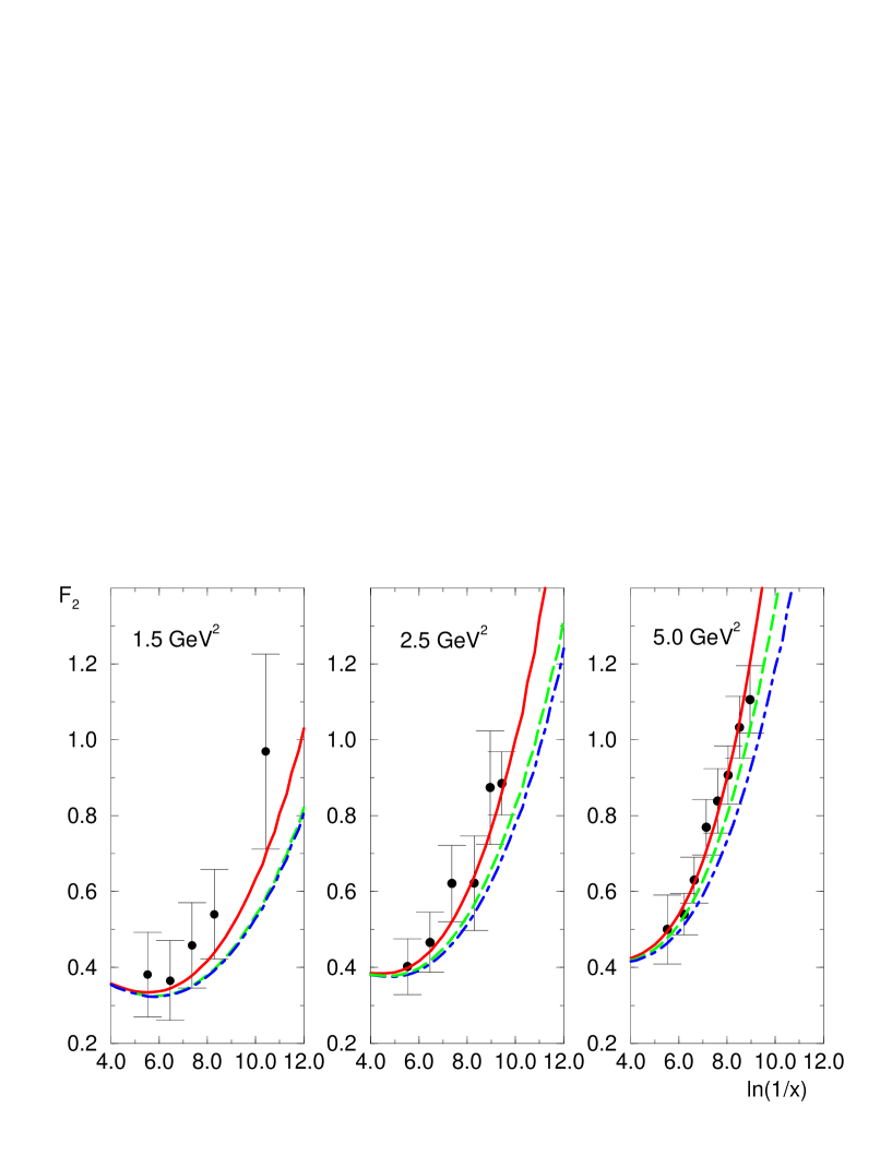
Figure 1: The $F_{2}$ structure function as a function of the variable $ln(\frac{1}{x})$ for different virtualities. Data from H1 [30]. The solid curve corresponds to GRV, the dashed curve to SC in the quark sector, the long-short dashed curve to SC in both quark and gluon sectors.

In Fig. 1 we present our results for the $F_{2}$ structure function as a function of the variable $ln\,(\frac{1}{x})$ for different virtualities. We have used $R^{2}=5\,GeV^{-2}$ in these calculations. In the next section the $R$ dependence of our results is analysed. We present our results using the expression (15) (quark sector) and using the solution of the equation (16) as input in the first term of (15) (quark + gluon sector). The predictions of the GRV parametrization are also shown. We consider the HERA data at low $Q^{2}$ since for $Q^{2}>6\,GeV^{2}$ the SC start to fall down (For a discussion of the SC to $F_{2}$ considering the quark sector see [24, 29]). We can see that at small values of $Q^{2}$ the predictions for $F_{2}$ considering the quark and the quark-gluon sector are approximately identical. However, for larger values of $Q^{2}$ the predictions of the quark-gluon sector disagree with the H1 data [30]. Therefore, the contribution of the gluon shadowing to $F_{2}$ in an eikonal approach superestimates the shadowing corrections at large $Q^{2}$ values.

In Fig. 2 we present our results for the SC in the $\frac{dF_{2}(x,Q^{2})}{dlogQ^{2}}$ as a function of $x$. The ZEUS data points [12] correspond to different $x$ and $Q^{2}$ value. The $(x,Q^{2})$ points are averaged values obtained from each of the experimental data distribution bins. Only the data points with $<Q^{2}>\,\geq 0.52\,GeV^{2}$ and $x<10^{-1}$ were used here.

The SC are estimated considering the expression (17) (quark sector) and using the solution of the equation (16) as input in the first term of (17) (quark + gluon sector). Moreover, the predictions of the traditional DGLAP framework, which at small values of $x$ is given by the expression (18) are also presented. We can see that the DGLAP predictions fail to describe the ZEUS data at small values of $x$ and $Q^{2}$. However we see that in the traditional framework (DGLAP + GRV94) a ’turn over’ is also present at small values of $x$ and $Q^{2}$. Basically, this occurs since the smaller $Q^{2}$ value used ($<Q^{2}>=0.52\,GeV^{2}$) is very near the initial virtuality of the GRV parametrization, where the gluon distribution is ’valence like’. Therefore the gluon distribution and the $F_{2}$ slope are approximately flat in this region. For the second smaller value of $Q^{2}$ used ($<Q^{2}>=1.1\,GeV^{2}$) the evolution length is larger, which implies that the gluon distribution (and the $F_{2}$ slope) already presents a steep behavior. The link between these points implies the ’turn over’ presented in Fig. 2. The main problem is that this ’turn over’ is higher than observed in the ZEUS data. This implies that $xG(x,Q^{2})$ differs from the previous standard expectations in the limit of small $x$ and $Q^{2}$. This effect is not observed in the $F_{2}$ structure function since it is inclusive to the behavior of the gluon distribution, which can be verified analysing the predictions of the distinct parametrizations. The gluon distribution predicted by these parametrizations differs in approximately 50 $\%$.

The prediction of the gluon sector, which is obtained using the solution of the expression (16) as input in (18) is also presented. We can see that at larger values of $Q^{2}$ and $x$ all predictions are approximately identical. However, at small values of $x$ and $Q^{2}$, the ZEUS data is not well described considering only the quark or the gluon sector to the SC. The contribution of the gluon shadowing is essential in the region of small values of $x$ and $Q^{2}$, i.e. a shadowed gluon distribution should be used as input in the eikonalized expression (17) in this kinematic region.

Our conclusion is that at small values of $x$ and $Q^{2}$ it should be considered the contribution of the gluon shadowing to estimate the SC to $F_{2}$ and its slope in the eikonal approach. While for $F_{2}$ the contribution of the gluon shadowing may be disregarded, it is essential for the $F_{2}$ slope. The $\frac{dF_{2}(x,Q^{2})}{dlogQ^{2}}$ data show that a consistent approach should consider both contributions at small $x$ and $Q^{2}$.

Before we conclude this section some comments are in order. We show that the $\frac{dF_{2}(x,Q^{2})}{dlogQ^{2}}$ data can be successfully described considering the shadowing corrections in the quark and gluon sectors. A similar conclusion was obtained in [10, 11], where the eikonal approach was also used to estimate the SC in the quark and gluon sectors, but a distinct procedure was used to estimate the SC for the $F_{2}$ slope. In [11] damping factors are calculated separately for both sectors and applied to the standard DGLAP predictions. The behavior of the gluon distribution at small values of $Q^{2}$ was modeled separately, since the gluon distribution (14) vanish for $Q^{2}=Q_{0}^{2}$. This procedure introduces a free parameter $\mu^{2}$, beyond the usual ones used in the eikonal approach ($Q_{0}^{2},\,R^{2}$). The distinct procedure proposed here estimates the observables directly within the eikonal approach and the shadowing corrections in the different sectors are calculated within the same approach. In our calculations there are only two free parameters: (i) the cutoff ($Q_{0}^{2}=0.4\,GeV^{2}$) in order to eliminate the long distance contribution, and (ii) the radius $R$ ($R^{2}=5\,GeV^{-2}$). The choice of these parameters is associated with the initial virtuality of the GRV parametrization used in our calculations, and the estimates obtained using the HERA data on diffractive photoproduction of $J/\Psi$ vector meson (see discussion in the next section) respectively [15, 16]. In our procedure the region of small values of $Q^{2}\approx Q_{0}^{2}$ is determined by the behavior of the GRV parameterization in this region, since we are using the eq. (16) to calculate the gluon distribution. For $Q^{2}=Q_{0}^{2}$ the two first terms of (16) vanish and the gluon distribution is described by the GRV parameterization, i.e. $xG(x,Q_{0}^{2})=xG(x,Q_{0}^{2})\mbox{[GRV]}$.

The eikonal approach describes the ZEUS data, as well as the DGLAP evolution equations using modified parton distributions. Recently, the MRST group [31] has proposed a different set of parton parametrizations which consider a initial ’valence-like’ gluon distribution. This parametrization allows to describe the $F_{2}$ slope data without an unconventional effect. This occurs because there is a large freedom in the initial parton distributions and the initial virtuality used in these parametrizations. We believe that only a comprehensive analysis of distinct observables ($F_{L},\,F_{2}^{c},\,\frac{dF_{2}(x,Q^{2})}{dlogQ^{2}}$) will allow a more careful evaluation of the shadowing corrections at small $x$ [9, 29].

3 The radius dependence of the shadowing corrections

The value of SC crucially depends on the size of the target [14]. In pQCD the value of $R$ is associated with the coupling of the gluon ladders with the proton, or to put it in another way, on how the gluons are distributed within the proton. $R$ may be of the order of the proton radius if the gluons are distributed uniformly in the whole proton disc or much smaller if the gluons are concentrated, i.e. if the gluons in the proton are confined in a disc with smaller radius than the size of the proton.

Considering the expression (8), assuming $\Omega_{q\overline{q}}<1$ and expanding the expression to ${\cal{O}}(\Omega^{2})$ we obtain

$$F_{2}(x,Q^{2})=\frac{1}{2\pi^{3}}\sum_{u,d,s}e_{f}^{2}\int_{\frac{1}{Q^{2}}}^{\frac{1}{Q_{0}^{2}}}\frac{d^{2}r_{t}}{r_{t}^{4}}\int d^{2}b_{t}\left\{\frac{1}{2}\Omega_{q\overline{q}}-\frac{1}{8}\Omega^{2}_{q\overline{q}}\right\}\,\,.$$ (19)

Using the factorization of the opacity and the normalization of the profile function we can write $F_{2}$ as

$$F_{2}(x,Q^{2})=\frac{1}{2\pi^{3}}\sum_{u,d,s}e_{f}^{2}\int_{\frac{1}{Q^{2}}}^{\frac{1}{Q_{0}^{2}}}\frac{d^{2}r_{t}}{r_{t}^{4}}\left\{\frac{1}{2}\overline{\Omega_{q\overline{q}}}-\frac{1}{8}\overline{\Omega_{q\overline{q}}}^{2}\int d^{2}b_{t}S^{2}(b_{t})\right\}\,\,.$$ (20)

The second term of the above equation represents the first shadowing corrections for the $F_{2}$ structure function. Assuming a Gaussian parametrization for the profile function we obtain that the screening is inversely proportional to the radius. Therefore the shadowing corrections are strongly associated with the distributions of the gluons within the proton. In this section we estimate the radius dependence of the shadowing corrections, considering the $F_{2}$ and $\frac{dF_{2}(x,Q^{2})}{dlogQ^{2}}$ data. First we explain why the radius is expected to be smaller than the proton radius.

Consider the first order contribution to the shadowing corrections, where two ladders couple to the proton. The ladders may be attached to different constituents of the proton or to the same constituent. In the first case the shadowing corrections are controlled by the proton radius, while in the second case these corrections are controlled by the constituent radius, which is smaller than the proton radius. Therefore, on the average, we expect that the radius will be smaller than the proton radius. Theoretically, $R^{2}$ reflects the integration over $b_{t}$ in the first diagrams for the SC.

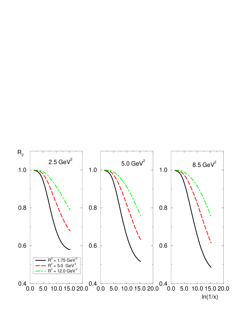
Figure 3: The ratio $R_{2}=\frac{F_{2}(x,Q^{2})\mbox{[Eq. (\ref{diseik2})]}}{F_{2}(x,Q^{2})\mbox{[GRV]}}$ as a function of the variable $ln(\frac{1}{x})$ for different virtualities and radii.

In Fig. 3 we present the ratio

$$R_{2}=\frac{F_{2}(x,Q^{2})\mbox{[Eq. (\ref{f2})]}}{F_{2}(x,Q^{2})\mbox{[GRV]}}\,\,,$$ (21)

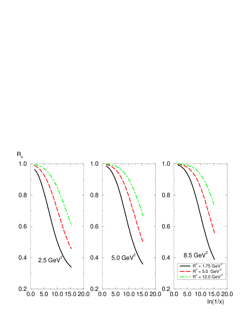
Figure 4: The ratio $R_{s}=\frac{\frac{dF_{2}(x,Q^{2})}{dlogQ^{2}}\mbox{[Eq. (\ref{df2eik})]}}{\frac{dF_{2}(x,Q^{2})}{dlogQ^{2}}\mbox{[GRV]}}$ as a function of the variable $ln(\frac{1}{x})$ for different virtualities and radii.

where $F_{2}(x,Q^{2})[\mbox{GRV}]=\sum_{u,d,s}e_{f}^{2}\,[xq(x,Q^{2})+x\overline{q}(x,Q^{2})]+F_{2}^{c}(x,Q^{2})$ is calculated using the GRV parametrization. For the treatment of the charm component of the structure function we consider the charm production via boson-gluon fusion [13]. In this paper we assume $m_{c}=1.5\,GeV$. In Fig. 4 we present the ratio

$$R_{s}=\frac{\frac{dF_{2}(x,Q^{2})}{dlogQ^{2}}\mbox{[Eq. (\ref{df2})]}}{\frac{dF_{2}(x,Q^{2})}{dlogQ^{2}}\mbox{[GRV]}}\,\,.$$ (22)

The function $\frac{dF_{2}(x,Q^{2})}{dlogQ^{2}}\mbox{[GRV]}$ was calculated using the expression (18) and the GRV parametrization. Our results are presented as a function of $ln(\frac{1}{x})$ at different virtualities. We can see that the SC are larger in the ratio $R_{s}$ and that our predictions of SC are strongly dependent of the radius $R$. Moreover, we see clearly the SC behavior inversely proportional with the radius.

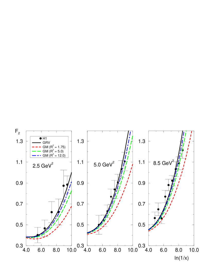
Figure 5: The $F_{2}$ structure function as a function of the variable $ln(\frac{1}{x})$ for different virtualities and radii. Only the shadowing corrections in the quark sector are considered. Data from H1 [30].

In Fig. 5 we compare our predictions for the SC in the $F_{2}$ structure function and the H1 data [30] as a function of $ln(\frac{1}{x})$ at different virtualities and some values of the radius. Our goal is not a best fit of the radius, but eliminate some values of radius comparing the predictions of the eikonal approach and HERA data. We consider only the quark sector in the calculation of SC, which is a good approximation in this observable, as shown in the previous section. The choice $R^{2}=1.5\,GeV^{2}$ does not describe the data, i.e. the data discard the possibility of very large SC in the HERA kinematic region. However, there are still two possibilities for the radius which reasonably describe the $F_{2}$ data. To discriminate between these possibilities we must consider the behavior of the $F_{2}$ slope.

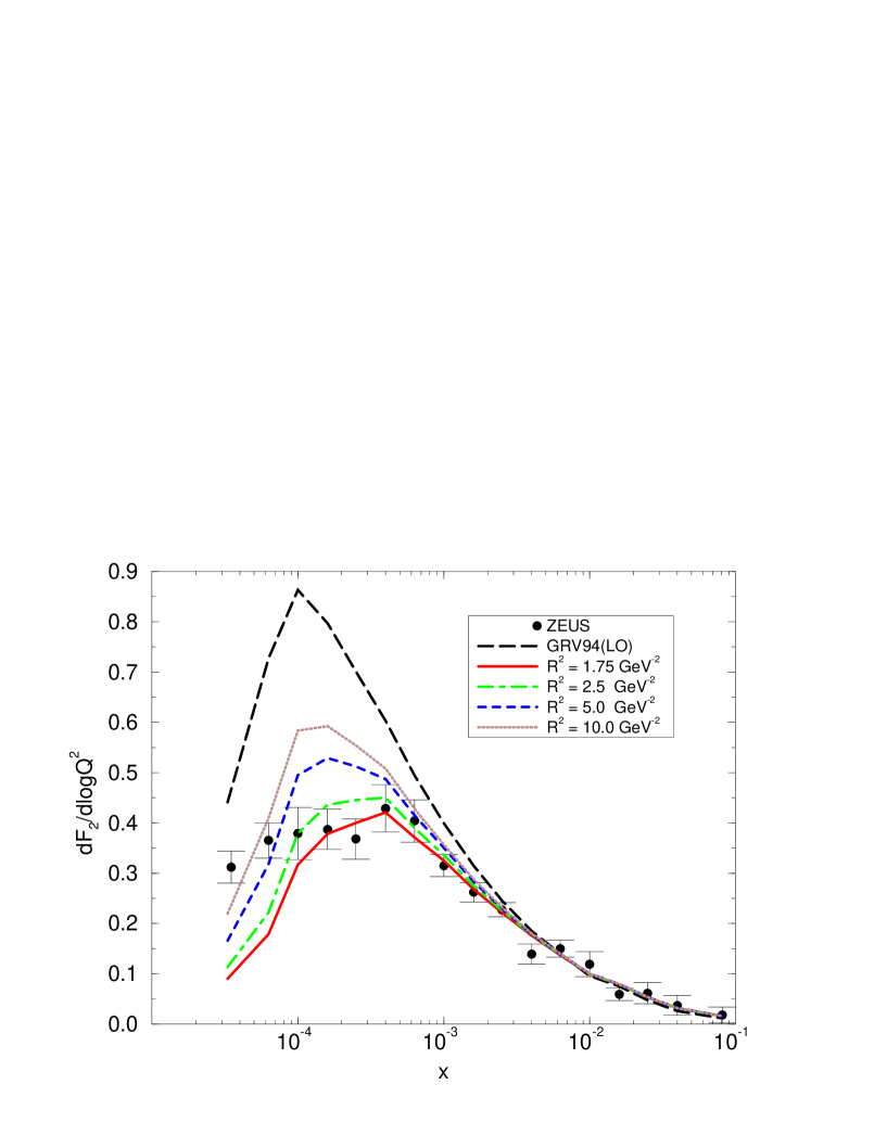
Figure 6: The $F_{2}$ slope as a function of the variable $x$ for different radii. Only the shadowing corrections in the quark sector are considered. Data from ZEUS [12]. The data points correspond to a different $x$ and $Q^{2}$ value.

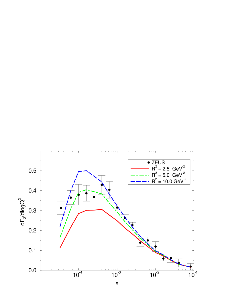
Figure 7: The $F_{2}$ slope as a function of the variable $x$ for different radii. The shadowing corrections in the gluon-quark sector are considered. Data from ZEUS [12]. The data points correspond to a different $x$ and $Q^{2}$ value.

In Fig. 6 we present our results for $\frac{dF_{2}(x,Q^{2})}{dlogQ^{2}}$ considering the SC only in the quark sector. Although in the previous section we have demonstrate that the contributions of the quark and gluon sectors should be considered, here we will test other possibilities to describe the data: the dependence on the radius $R$. Our results show that the best fit of the data occurs at small values of $R^{2}$, which are discarded by the $F_{2}$ data. Therefore, in agreement with our previous conclusions, we must consider a general approach to describe consistently the $F_{2}$ and $\frac{dF_{2}(x,Q^{2})}{dlogQ^{2}}$ data. In Fig. 7 we present our results for $\frac{dF_{2}(x,Q^{2})}{dlogQ^{2}}$ considering the SC in the gluon and quark sector for different values of $R^{2}$, calculated using the general approach proposed in the previous section. The best result occurs for $R^{2}=5\,GeV^{-2}$, which also describes the $F_{2}$ data.

The value for the squared radius $R^{2}=5\,GeV^{-2}$ obtained in our analysis agrees with the estimates obtained using the HERA data on diffractive photoproduction of $J/\Psi$ meson [15, 16]. Indeed, the experimental values for the slope are $B_{el}=4\,GeV^{-2}$ and $B_{in}=1.66\,GeV^{-2}$ and the cross section for $J/\Psi$ diffractive production with and without photon dissociation are equal. Neglecting the $t$ dependence of the pomeron-vector meson coupling the value of $R^{2}$ can be estimated [19]. It turns out that $R^{2}\approx 5\,GeV^{-2}$, i.e., approximately 2 times smaller than the radius of the proton.

As an additional comment let us say that the SC to $F_{2}$ and its slope may also be analysed using a two radii model for the proton [10]. This analysis is motivated by the large difference between the measured slopes in elastic and inelastic diffractive leptoproduction of vector mesons in DIS. An analysis using the two radii model for the proton is not a goal of this paper, since a definite conclusion on the correct model is still under debate.

The summary of this point is that the analysis of the $F_{2}$ and $\frac{dF_{2}(x,Q^{2})}{dlogQ^{2}}$ data using the eikonal model implies that the gluons are not distributed uniformly in the whole proton disc, but behave as concentrated in smaller regions. This conclusion motivates an analysis of the jet production, which probes smaller regions within the proton, using an approach which considers the shadowing corrections.

4 A screnning boundary

The common feature of the BFKL and DGLAP equations is the steep increase of the cross sections as $x$ decreases. This steep increase cannot persist down to arbitrary low values of $x$ since it violates a fundamental principle of quantum theory, i.e. the unitarity. In the context of relativistic quantum field theory of the strong interactions, unitarity implies the cross section of a hadronic scattering reaction cannot increase with increasing energy $s$ above $log^{2}\,s$: the Froissart’s theorem [17]. The Froissart bound cannot be proven for off-mass-shell amplitudes [18], which is the case for deep inelastic scattering [32]. Our goal in this section is by using the $s$-channel unitarity (6) and the eikonal approach to estimate a superior limit from which the shadowing corrections cannot be disregarded in $F_{2}$ and its slope.

Considering the expression (8) for the $F_{2}$ structure function, we can write a $b_{t}$ dependent structure function given by

$$F_{2}(x,Q^{2},b_{t})=\frac{1}{2\pi^{3}}\sum_{u,d,s}e_{f}^{2}\int_{\frac{1}{Q^{2}}}^{\frac{1}{Q_{0}^{2}}}\frac{dr^{2}_{t}}{r_{t}^{4}}\left\{1-e^{-\frac{1}{2}\Omega_{q\overline{q}}(x,r_{t},b_{t})}\right\}\,\,.$$ (23)

The relation between the opacity and the gluon distribution (9) obtained in [19], is valid in the kinematical region where $\Omega\ll 1$. In the eikonal approach for pQCD we make the assumption that the relation (9) is valid in all kinematic region. To obtain an estimate of the region where the SC are important we consider a superior limit for the expression (23), which occurs for $\Omega\gg 1$. In this limit the second term in the above equation can be disregarded. As the shadowing terms are negative and reduce the growth of the $F_{2}$ structure function, disregarding the shadowing terms we are estimating a superior limit for the region where these terms are not important, i.e. a screnning boundary which establishes the region where the shadowing corrections are required to calculate the observables.

The $b_{t}$ dependent structure function in the limit $\Omega\gg 1$ is such that

$$F_{2}(x,Q^{2},b_{t})<\frac{1}{2\pi^{3}}\sum_{u,d,s}e_{f}^{2}\int_{\frac{1}{Q^{2}}}^{\frac{1}{Q_{0}^{2}}}\frac{dr^{2}_{t}}{r_{t}^{4}}\,\,.$$ (24)

Making the assumption that the $b_{t}$ dependence of the structure function is factorized [19]:

$$F_{2}(x,Q^{2},b_{t})=F_{2}(x,Q^{2})\,S(b_{t})\,\,,$$

and considering a Gaussian parametrization for the profile function and its value for $b_{t}=0$ we get ($n_{f}=3$)

$$F_{2}(x,Q^{2})<\frac{R^{2}}{3\pi^{2}}\int_{\frac{1}{Q^{2}}}^{\frac{1}{Q_{0}^{2}}}\frac{dr^{2}_{t}}{r_{t}^{4}}\,\,.$$ (25)

As a result

$$F_{2}(x,Q^{2}) < \frac{R^{2}}{3\pi^{2}}(Q^{2}-Q_{0}^{2})$$ (26)

$$< \frac{R^{2}Q^{2}}{3\pi^{2}}\,\,.$$

The above limit is our estimate for the screnning boundary for the $F_{2}$ structure function.

The screnning boundary for the $F_{2}$ slope is straightforward from the expression (24). We get

$$\frac{dF_{2}(x,Q^{2})}{dlogQ^{2}}<\frac{R^{2}Q^{2}}{3\pi^{2}}\,\,.$$ (27)

This expression agrees with the expression obtained in [19].

Clearly expressions (26) and (27) serve only as a rough prescription for estimating the region where the corrections required by unitarity cannot be disregarded. A more rigorous treatment would be desirable, but remains to be developed.

Using the above expressions we can make an analysis of HERA data. We use $R^{2}=5\,GeV^{-2}$ in the calculations. In Fig. 8 we compare our predictions with the $F_{2}$ data from the H1 collaboration. We can see that data at larger values of $Q^{2}$ ($Q^{2}\geq 8.5\,GeV^{2}$) do not violate the limit (26). However, the data at smaller values of $Q^{2}$ and $x$ violate this limit. This indicates that we should consider the SC for this kinematical region. In Fig. 9 we present our results for the $F_{2}$ slope. We see that the data for small $Q^{2}$ and $x$ ($Q^{2}\leq 2.5\,GeV^{2}$, $x\leq 10^{-4}$) violate the limit (27), stressing the need of the shadowing corrections. Therefore for small values of $x$ and $Q^{2}$ the observables must be calculated using an approach which takes them into account.

5 Summary

In this paper we have presented our analysis of the shadowing corrections in the scaling violations using the eikonal approach. We shown that the $\frac{dF_{2}(x,Q^{2})}{dlogQ^{2}}$ data can be described successfully considering the shadowing corrections in the quark and gluon sectors. Furthermore, we have considered the radius dependence of these corrections and an unitarity boundary. From the analysis of the $R$ dependence of the SC in the eikonal approach we have shown that the value $R^{2}=5\,GeV^{-2}$ allows to describe the HERA data. This value agrees with the estimate obtained independently in the diffractive $J/\Psi$ photoproduction. Using the eikonal approach and the assumption of $b_{t}$ factorization of the $F_{2}$ structure function a screnning boundary is analysed. This boundary constrains the region where the corrections required by unitarity may be disregarded; or in other words, a limit for applicablity of standard perturbative QCD framework. We have shown that the HERA data at small $x$ and $Q^{2}$ violate this limit, which implies that the shadowing corrections are important in the HERA kinematic region.

Our conclusion is that the shadowing effect is important already at HERA kinematic region. We believe that the analysis of distinct observables ($F_{L},\,F_{2}^{c},\,\frac{dF_{2}(x,Q^{2})}{dlogQ^{2}}$) at small values of $x$ and $Q^{2}$ will allow to evidentiate the shadowing corrections.

Figure 2: The $F_{2}$ slope as a function of the variable $x$. Data from ZEUS [12]. The data points correspond to a different $x$ and $Q^{2}$ value. The solid curve corresponds to SC in both quark and gluon sectors.

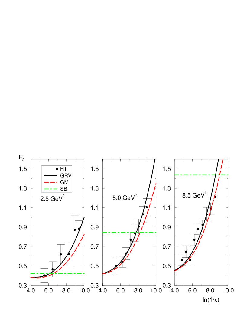
Figure 8: Screnning boundary to the $F_{2}$ structure function. For points above the boundary the corrections cannot be disregarded. Data from H1 [30].

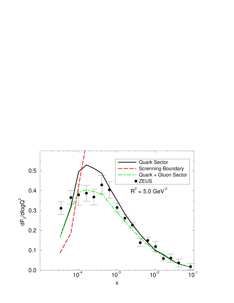
Figure 9: Screnning boundary to the $F_{2}$ slope. For points above the boundary the corrections cannot be disregarded. Data from ZEUS [12].

References

- [1] A. M. Cooper-Sarkar, R.C.E. Devenish and A. De Roeck, Int. J. Mod. Phys A13, 3385 (1998).
- [2] Yu. L. Dokshitzer, Sov. Phys. JETP 46, 641 (1977); G. Altarelli and G. Parisi, Nucl. Phys. B126, 298 (1977); V. N. Gribov and L. N. Lipatov, Sov. J. Nucl. Phys 28, 822 (1978).
- [3] E. A. Kuraev, L. N. Lipatov and V.S. Fadin, Phys. Lett B60, 50 (1975); Sov. Phys. JETP 44, 443 (1976); Sov. Phys. JETP 45, 199 (1977); Ya. Balitsky and L. N. Lipatov, Sov. J. Nucl. Phys. 28, 822 (1978).
- [4] L. V. Gribov, E. M. Levin and M. G. Ryskin, Phys. Rep. 100, 1 (1983).
- [5] Future Physics at HERA. Proceedings of the Workshop 1995/1996, Hamburg, Germany, 1996, edited by G. Ingelman et al. (DESY, Hamburg, 1996).
- [6] R. Ball and S. Forte, Phys. Lett. B335, 77 (1994).
- [7] J. Kwiecinski, A. D. Martin and A. M. Stasto, Phys. Rev. D56, 3991 (1997).
- [8] J. Bartels, J. Blümlein and G. A. Schuler, Z. Phys. C50, 91 (1991); A. Askew et al., Phys. Rev. D47, 3775 (1993); W. Zhu et al., Nucl. Phys., 183 B449 (1995).
- [9] A. L. Ayala, M. B. Gay Ducati and V. P. Gonçalves, Phys. Rev. D (in press), hep-ph/9807263.
- [10] E. Gotsman, E. Levin and U. Maor. Phys. Lett B425, 369 (1998).
- [11] E. Gotsman et al., hep-ph/9808257.
- [12] M. Derrick et al. (ZEUS COLLABORATION), hep-ph/9809005.
- [13] M. Gluck, E. Reya and A. Vogt, Z. Phys. C67, 433 (1995).
- [14] A. H. Mueller, Nucl. Phys. B (Proc. Suppl.) 18C, 125 (1990); J. Bartels, A. De Roeck and M. Loewe, Z. Phys. C54, 635 (1992).
- [15] M. Derrick et al. (ZEUS COLLABORATION), Phys. Lett B350, 120 (1995).
- [16] S. Aid et al. (H1 COLLABORATION), Nucl. Phys. B472, 3 (1996).
- [17] M. Froissart, Phys. Rev.123, 1053 (1961).
- [18] C. Lopez and F. J. Yndurain, Phys. Rev. Lett. 44, 1118 (1980).
- [19] A. L. Ayala, M. B. Gay Ducati and E. M. Levin, Phys. Lett. B388, 188 (1996).
- [20] V. N. Gribov, Sov. Phys. JETP 30, 709 (1970).
- [21] N. Nikolaev and B. G. Zakharov, Z. Phys. C49, 607 (1990); S. J. Brodsky, A. Hebecker and E. Quack, Phys. Rev. D55, 2584 (1997).
- [22] W. Buchmuller, A. Hebecker and M. F. McDermott, Nucl. Phys. B487, 283 (1997).
- [23] R. J. Glauber, Phys. Rev. 100, 242 (1955); R. C. Arnold, Phys. Rev. 153, 1523 (1967); T. T. Chou and C. N. Yang, Phys. Rev. 170, 1591 (1968).
- [24] A. L. Ayala, M. B. Gay Ducati and E. M. Levin, Nucl. Phys. B511, 355 (1998).
- [25] A. D. Martin, R. G. Roberts and W. J. Stirling, Phys. Lett. B387, 419 (1996).
- [26] H. L. Lai et al., Phys. Rev. D55, 1280 (1997).
- [27] A. L. Ayala, M. B. Gay Ducati and E. M. Levin, Nucl. Phys. B493, 305 (1997).
- [28] A. H. Mueller, Nucl. Phys. B335, 115 (1990).
- [29] A. L. Ayala, M. B. Gay Ducati and E. M. Levin, Eur. Phys. J. C (in press), hep-ph/9710539.
- [30] S. Aid et al. (H1 COLLABORATION), Nucl. Phys. B470, 3 (1996).
- [31] A. D. Martin et al., Eur. Phys. J. C4, 463 (1998).
- [32] E. Gotsman, E. Levin and U. Maor, Eur. Phys. J. C5, 303 (1998).