CLNS98/1598
Sixth-Order Vacuum-Polarization Contribution
to the Lamb Shift of the Muonic Hydrogen

Abstract

The sixth-order electron-loop vacuum-polarization contribution to the $2P_{1/2}-2S_{1/2}$ Lamb shift of the muonic hydrogen ($\mu^{-}p^{+}$ bound state) is evaluated numerically. Our result is 0.007608 (1) meV. This eliminates the largest theoretical uncertainty. Combined with the proposed precision measurement of the Lamb shift it will lead to a precise determination of the proton charge radius.

The muonic hydrogen, the $\mu^{-}p^{+}$ bound state, differs from the ordinary hydrogen atom in two important respects. One is that the vacuum-polarization effect is much more important than other radiative corrections. The other is that it is more sensitive to the hadronic structure of the proton. Thus it provides a means of testing aspects of QED significantly different from those of the hydrogen atom.

The muonic hydrogen has a long-lived $2S$ meta-stable state. This makes it possible to measure the $2P_{1/2}-2S_{1/2}$ Lamb shift to about 10 ppm level using the phase-space compressed muon beam technique [1]. At present, however, theoretical precision is limited to about 50 ppm. This uncertainty comes mainly from the unknown contribution $\Delta E^{(6)}$ of the sixth-order electron vacuum-polarization effect [2].

In this paper we report the result of our evaluation of $\Delta E^{(6)}$. Our result is

$$\Delta E^{(6)} = 0.120~{}045~{}(12)~{}m_{r}(Z\alpha)^{2}\left({\alpha\over\pi}\right)^{3}$$ (1)

$$= 0.007~{}608~{}(1)~{}~{}\mbox{meV},$$ (2)

where $Z=1$ for the proton and $m_{r}$ is the reduced mass of the $\mu^{-}p^{+}$ system:[3]

$$m_{r} = {m_{\mu}m_{p}\over m_{\mu}+m_{p}}=94.964~{}485~{}(28)~{}\mbox{MeV},$$ (3)

$$m_{\mu} = 105.658~{}389(34)~{}~{}\mbox{MeV},$$ (4)

$$m_{p} = 938.272~{}31(28)~{}~{}\mbox{MeV}~{}~{}.$$ (5)

We have also evaluated the main part of $\Delta E^{(6)}$ using the Padé approximation of vacuum-polarization function [4]. The result (36) is in good agreement with the direct calculation (34).

The contribution to the $2P_{1/2}-2S_{1/2}$ Lamb Shift of the muonic hydrogen due to the effect of the electron-loop vacuum-polarization on a single Coulomb photon can be expressed as an integral over the vacuum-polarization function $\Pi(q^{2})$. Here $q$ may be either space-like or time-like. The first choice ($q^{2}<0$) leads to the integral

$$\Delta^{(I)}E=\int{d^{3}q\over(2\pi)^{3}}\tilde{\rho}(a^{2}){-4\pi Z\alpha\over\vec{q}^{2}}\left[-\Pi(-\vec{q}^{2})\right]~{}.$$ (6)

Here $\tilde{\rho}$ is equal to $\tilde{\rho}_{2P}-\tilde{\rho}_{2S}$, $\tilde{\rho}_{2P}$ and $\tilde{\rho}_{2S}$ being Fourier transforms of squares of non-relativistic Coulomb wave functions for the $2P$ and $2S$ states:

$$\tilde{\rho}_{2P(2S)}=\int d^{3}r|\phi_{2P(2S)}(\vec{r})|^{2}e^{-i\vec{q}\cdot\vec{r}}.$$ (7)

Carrying out the integration we obtain

$$\tilde{\rho}_{2P}={1-a^{2}\over(1+a^{2})^{4}}~{},~{}~{}~{}~{}\tilde{\rho}_{2S}={1-3a^{2}+2a^{4}\over(1+a^{2})^{4}}~{},$$ (8)

where $a=|\vec{q}|/(Z\alpha m_{r})$ and $\tilde{\rho}_{2P}$ is averaged over three degenerate states.

The second choice ($q^{2}>0$) gives rise to the integral [2]

$$\Delta^{(II)}E=m_{r}(Z\alpha)^{2}\int_{4}^{\infty}dtu(t){\beta^{2}\over 2(1+\beta\sqrt{t})^{4}}~{},$$ (9)

where

$$\beta={m_{e}\over m_{r}\alpha}=0.737~{}383~{}76~{}(30)$$ (10)

and

$$u(t)={1\over\pi}Im\Pi(q^{2}=tm_{e}^{2})~{}~{}.$$ (11)

Although Eqs. (6) and (9) are analytically equivalent, they are totally different from the viewpoint of numerical integration. Thus they provide a useful check whenever both real and imaginary parts of $\Pi$ are available. For diagrams containing several vacuum-polarization loops in one Coulomb photon line, Eqs. (6) and (9) must be modified accordingly. Insertion of vacuum polarization loops in several Coulomb photon lines can be handled by the non-relativistic bound-state perturbation theory.

FIG. 1.: Three second-order vacuum-polarization diagrams inserted in the Coulomb photon line exchanged by the muon and the proton.

Let us first consider insertion of three second-order vacuum-polarizations in a Coulomb photon (see Fig.1). The contribution $\Pi^{(p2:3)}(q^{2})$ of this improper diagram can be expressed in terms of the second-order vacuum-polarization function $\Pi^{(2)}(q^{2})$ as

$$\Pi^{(p2:3)}(q^{2})=(\Pi^{(2)}(q^{2}))^{3}~{},$$ (12)

where $\Pi^{(2)}$ is known analytically and has the spectral function

$$u^{(2)}(t)={1\over 3}{\alpha\over\pi}\sqrt{1-{4m_{e}^{2}\over q^{2}}}\left(1+{2m_{e}^{2}\over q^{2}}\right),~{}~{}~{}q^{2}\geq 4m_{e}^{2}.$$ (13)

Substituting $\Pi^{(p2:3)}$ in Eq. (6) and evaluating the integral numerically, we find

$$\Delta^{(I)}E^{(p2:3)}=0.006~{}253~{}4~{}(6)~{}m_{r}(Z\alpha)^{2}\left({\alpha\over\pi}\right)^{3}~{}.$$ (14)

The result of the second method (9) agrees with (14):

$$\Delta^{(II)}E^{(p2:3)}=0.006~{}253~{}9~{}(10)~{}m_{r}(Z\alpha)^{2}\left({\alpha\over\pi}\right)^{3}~{}.$$ (15)

Another evaluation of $\Delta^{(I)}E^{(p2:3)}$ using the parametric-integral form of $\Pi^{(2)}$ given in Ref. [6] leads to

$$\Delta^{(I)}E^{(p2:3)}=0.006~{}253~{}8~{}(8)~{}m_{r}(Z\alpha)^{2}\left({\alpha\over\pi}\right)^{3}~{}.$$ (16)

FIG. 2.: Insertion of one second- and one fourth-order vacuum-polarization diagrams in the Coulomb photon line exchanged by the muon and the proton.

The next contribution comes from diagrams involving one second-order and one fourth-order vacuum-polarization insertions (see Fig. 2). This contribution is given in terms of

$$\Pi^{(p4p2)}(q^{2})=-2\Pi^{(2)}(q^{2})\Pi^{(4)}(q^{2})~{},$$ (17)

where $\Pi^{(4)}$ is the fourth-order vacuum-polarization function [7]. Substituting $\Pi^{(4)}$ into Eqs. (6) and (9) we obtain

$$\Delta^{(I)}E^{(p4p2)}=0.046~{}248~{}(5)~{}m_{r}(Z\alpha)^{2}\left({\alpha\over\pi}\right)^{3}~{},$$ (18)

and

$$\Delta^{(II)}E^{(p4p2)}=0.046~{}243~{}(16)~{}m_{r}(Z\alpha)^{2}\left({\alpha\over\pi}\right)^{3}~{}.$$ (19)

We also evaluated $\Delta^{(I)}E^{(p4p2)}$ using the parametric-integral form of $\Pi^{(4)}$ [6]:

$$\Delta^{(I)}E^{(p4p2)}=0.046~{}250~{}(2)~{}m_{r}(Z\alpha)^{2}\left({\alpha\over\pi}\right)^{3}~{}.$$ (20)

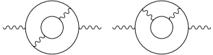
FIG. 3.: Sixth-order vacuum-polarization diagrams with a second-order vacuum-polarization inserted in the fourth-order vacuum-polarization diagrams.

The third contribution comes from the sixth-order vacuum-polarization term $\Pi^{(p4(p2))}$ obtained by inserting a second-order vacuum-polarization loop in the fourth-order vacuum-polarization diagram (see Fig.3). The form of $\Pi^{(p4(p2))}$ convenient for numerical integration is as integral over Feynman parameters [6]. This can be done easily by adapting to the Lamb shift the program written previously for the electron $g-2$ [8]. This leads to

$$\Delta^{(I)}E^{(p4(p2))}=0.013~{}628~{}(6)~{}m_{r}(Z\alpha)^{2}\left({\alpha\over\pi}\right)^{3}~{}.$$ (21)

The $\overline{\rm MS}$ renormalized imaginary part of $\Pi^{(p4(p2))}$ is known in a two dimensional integral form [9]. Converting it to the on-shell renormalized one and using Eq. (9), we obtained

$$\Delta^{(II)}E^{(p4(p2))}=0.013~{}626~{}(1)~{}m_{r}(Z\alpha)^{2}\left({\alpha\over\pi}\right)^{3}~{}.$$ (22)

FIG. 4.: Sixth-order vacuum-polarization diagrams with a single electron loop.

The fourth contribution comes from the sixth-order vacuum-polarization diagrams with a single electron loop. The exact form of this contribution is known only in a parametric-integral form [6]. Its imaginary part is not available in a form convenient for numerical work. We have therefore evaluated it using Eq. (6) only. There are eight topologically distinct diagrams (see Fig.4). Each diagram can be written as a sum of various divergent terms and a finite part $\Delta\Pi^{(6i)}$, where $i=a,b,...,h$. After renormalization the sum of these diagrams is free from any divergence and can be written as [6]

$$\Pi^{(p6)} = 2(\Delta\Pi^{(6a)}+\Delta\Pi^{(6c)}+\Delta\Pi^{(6d)}+\Delta\Pi^{(6f)})$$ (23)

$$+ \Delta\Pi^{(6b)}+4\Delta\Pi^{(6e)}+\Delta\Pi^{(6g)}+\Delta\Pi^{(6h)}$$ (24)

$$- 4\Delta B_{2}\Pi^{(4)}-2[\Delta B_{4a}+\Delta L_{4x}+2\Delta L_{4c}$$ (25)

$$+ \Delta B_{4b}+\Delta L_{4l}+2\Delta L_{4s}+{3\over 2}(\Delta B_{2})^{2}]\Pi^{(2)}$$ (26)

$$- 2(\Delta\delta m_{4a}+\Delta\delta m_{4b})\Pi^{(2\ast)}~{},$$ (27)

where $\Delta B_{2},~{}\cdots$, are finite parts of renormalization constants and $\Pi^{(2)}$ and $\Pi^{(4)}$ are renormalized vacuum-polarization functions of second- and fourth-order, respectively. $\Pi^{(2\ast)}$ is the second-order vacuum-polarization function with a mass insertion vertex. Precise definitions of these functions are given in Ref. [10]. The numerical values of the coefficients of $\Pi^{(4)}$, $\Pi^{(2)}$ and $\Pi^{(2\ast)}$ are

$$\Delta B_{2} = {3\over 4}~{}{\alpha\over\pi}~{},$$ (28)

$$\Delta B_{4a}+~{}\cdots~{}+{3\over 2}(\Delta B_{2})^{2} = 0.871~{}680~{}(27)\biggl{(}{\alpha\over\pi}\biggr{)}^{2},$$ (29)

$$\Delta\delta m_{4a}+\Delta\delta m_{4b} = 1.906~{}340~{}(21)\biggl{(}{\alpha\over\pi}\biggr{)}^{2}~{},$$ (30)

where the last two are new evaluations. The Lamb Shift contributions from $\Pi^{(4)}$, $\Pi^{(2)}$, and $\Pi^{(2\ast)}$ can be easily obtained by numerical integration:

$$\Delta E^{(p4)} = 0.045~{}922~{}7~{}(4)~{}m_{r}(Z\alpha)^{2}\biggl{(}{\alpha\over\pi}\biggr{)}^{2}~{},$$ (31)

$$\Delta E^{(p2)} = 0.017~{}452~{}8~{}(3)~{}m_{r}(Z\alpha)^{2}{\alpha\over\pi}~{},$$ (32)

$$\Delta E^{(p2\ast)} = -0.009~{}001~{}8~{}(2)~{}m_{r}(Z\alpha)^{2}{\alpha\over\pi}.$$ (33)

The Lamb Shift contributions $\Delta E^{(p6a)},\cdots$, coming from the ultraviolet- and infrared-finite parts of diagrams $\Delta\Pi^{(6a)},\cdots$, are numerically evaluated. The results are summarized in Table I. The second and third columns list the results of integration carried out in double precision and quadruple precision, respectively. The purpose of the latter calculation is to see whether the former indicates sign of losing significant digits due to rounding-off, which we call $digit$-$deficiency$ problem and is the major source of uncertainty of on-the-computer renormalization [11]. The excellent agreement between two calculations shows that the estimated error of the former is not significantly affected by the $digit$-$deficiency$ problem and can be safely assumed to be mostly statistical. We therefore choose the double precision value, which has higher statistics, as our best estimate:

$$\Delta^{(I)}E^{(p6)}=0.017~{}410~{}(9)~{}m_{r}(Z\alpha)^{2}\left({\alpha\over\pi}\right)^{3}~{}.$$ (34)

As a cross-check, we also evaluated $\Delta E^{(p6)}$ using the Padé-approximation of the vacuum-polarization function from Ref. [4]. We did this using both methods I and II. The [2/3] and [3/2] Padé approximations give nearly identical results. Taking their average we obtain

$$\Delta^{(I)}E_{Pad\acute{e}}^{(p6)} = 0.017~{}414~{}9~{}(25)~{}m_{r}(Z\alpha)^{2}\left({\alpha\over\pi}\right)^{3},$$ (35)

$$\Delta^{(II)}E_{Pad\acute{e}}^{(p6)} = 0.017~{}414~{}9~{}(26)~{}m_{r}(Z\alpha)^{2}\left({\alpha\over\pi}\right)^{3}.$$ (36)

These results are consistent with each other and agree with (34) to three significant digits, or within one standard deviation of (34). Obviously either (34) or (36) has sufficient precision as far as comparison with experiment is concerned. Note, however, that the uncertainties given in (36) are those resulting from numerical treatment of the Padé approximation and do not include those caused by the Padé method itself. It is argued in a separate paper [11] that the uncertainty of the Padé model itself is about 0.001 percent and hence the true value will be found well within the uncertainties given in (36).

FIG. 5.: Representative sixth-order diagrams in which vacuum-polarization insertion occurs in two and three Coulomb photon lines. Vertical lines represent the muon moving in the Coulomb potential generated by the proton, which is indicated by a $``\times$”.

Thus far we considered only diagrams in which one Coulomb photon line is modified by the electron-loop vacuum polarization. Additional contributions of order $\alpha^{3}$ arise from the diagrams of Fig. 5 in which two and three Coulomb photons are modified by vacuum polarization. Their contributions to the Lamb shift can be found by the bound-state perturbation theory:

$$\Delta E({\rm Fig.5a}) = 0.009~{}166~{}(2)~{}m_{r}(Z\alpha)^{2}\left({\alpha\over\pi}\right)^{3},$$ (37)

$$\Delta E({\rm Fig.5b}) = 0.024~{}805~{}(3)~{}m_{r}(Z\alpha)^{2}\left({\alpha\over\pi}\right)^{3},$$ (38)

$$\Delta E({\rm Fig.5c}) = 0.002~{}535~{}(1)~{}m_{r}(Z\alpha)^{2}\left({\alpha\over\pi}\right)^{3}.$$ (39)

In this calculation we used the reduced non-relativistic Coulomb Green function for $2S$ and $2P$ states given by Eqs. (23) and (24) of Ref. [2].

Collecting (14), (18), (21), (34), and (39), we obtain the total contribution to the Lamb shift (2) due to the sixth-order vacuum-polarization effect.

Evaluation of various lower-order contributions to the $2P_{1/2}-2S_{1/2}$ Lamb shift ${\cal L}$ of the muonic hydrogen are summarized in Ref. [2]. In addition we have obtained the hadronic vacuum-polarization correction of 0.0113(3) meV following Ref. [12]. These results and our result (2) lead to the most precise theoretical prediction

$${\cal L}=(206.068~{}(2)-5.197~{}5~{}r_{p}^{2})~{}{\rm meV},$$ (40)

where $r_{p}$ is the proton charge radius in units of fm. The uncertainty in the first term of (40) is our estimate of theoretical error.

To improve the theoretical prediction further, it is necessary to have better estimate of the effect to the Lamb shift and hyperfine structure of the muonic hydrogen due to the proton’s internal structure beyond elastic form factors. Recently the proton polarizability correction to the hyperfine structure of the hydrogen and muonic hydrogen was obtained [13]. There are also references for ordinary hydrogen and deuterium [14, 15]. Unfortunately they are not directly applicable to the muonic hydrogen because of very different energy scale.

Measurement of ${\cal L}$ to 10 ppm, or 0.002 meV, will lead to improvement in the value of $r_{p}^{2}$ by an order of magnitude over those determined from the elastic scattering form factor measurements, making it possible to resolve the long-standing discrepancy between [16] and [17]. The new value of $r_{p}^{2}$ will also play an important role in testing the validity of QED in terms of high precision measurements of the hydrogen atom [18]. Another impact of accurate determination of $r_{p}^{2}$ will be to stimulate evaluation of $r_{p}^{2}$ from the lattice QCD more precise and reliable than those available at present [19].

We thank D. Taqqu for communicating about the proposed measurement of the Lamb shift of the muonic hydrogen. We thank K. Pachucki for pointing out the need to include the contribution of Fig. 5, for bringing our attention to Ref. [12]. We also thank K. Chetrykin, J. H. Kühn, R. Harlander, and M. Steinhauser for informing us of Ref. [9]. The work of T. K. is supported in part by the U. S. National Science Foundation. The work of M. N. is supported in part by the Grant-in-Aid (No. 10740123) of the Ministry of Education, Science, and Culture, Japan.

TABLE I.: Contributions to the $2P_{1/2}-2S_{1/2}$ muonic hydrogen Lamb shift from the sixth-order vacuum polarization diagrams with a single electron loop. The overall factor $m_{r}(Z\alpha)^{2}(\alpha/\pi)^{3}$ is omitted. The second and third columns give results of integration in double precision and quadruple precision, respectively. Their difference is listed in column 4.

Term	Doub. precis.	Quad. precis.	Difference
$\Delta E^{(6a)}$	0.044 769 (4)	0.044 739 (51)	0.000 030 (52)
$\Delta E^{(6b)}$	0.028 654 (4)	0.028 640 (35)	0.000 014 (36)
$\Delta E^{(6c)}$	-0.025 393 (3)	-0.025 368 (23)	- 0.000 025 (24)
$\Delta E^{(6d)}$	-0.026 376 (2)	-0.026 371 (21)	- 0.000 005 (22)
$\Delta E^{(6e)}$	0.151 356 (4)	0.151 334 (46)	0.000 022 (47)
$\Delta E^{(6f)}$	-0.067 139 (3)	-0.067 144 (30)	0.000 005 (31)
$\Delta E^{(6g)}$	0.019 536 (3)	0.019 540 (23)	- 0.000 004 (24)
$\Delta E^{(6h)}$	0.025 877 (2)	0.025 858 (22)	0.000 019 (23)

REFERENCES

- [1] D. Taqqu et al., Hyp. Int. 101/102, 599 (1996).
- [2] K. Pachucki, Phys. Rev. A 53, 2092 (1996).
- [3] C. Caso et al., Euro. Phys. J. C3, 1 (1998).
- [4] P. A. Baikov and D. J. Broadhurst, in New Computing Techniques in Physics Research IV, eds. B. Denby and D. Perret-Gallix (World Scientific, Singapore, 1995), pp. 167 -172.
- [5] G. P. Lepage, J. Comput. Phys. 27, 192 (1978).
- [6] T. Kinoshita and W. B. Lindquist, Phys. Rev. D 27, 853 (1983).
- [7] G. Källén and A. Sabry, K. Dan. Vidensk. Selsk. Mat.-Fys. Medd. 29, No. 17 (1955).
- [8] T. Kinoshita and W. B. Lindquist, Phys. Rev. D 27, 867 (1983).
- [9] K. G. Chetyrkin, A. H. Hoang, J. H. Kühn, M. Steinhauser and T. Teubner, Euro. Phys. J. C2, 137 (1998).
- [10] P. Cvitanović and T. Kinoshita, Phys. Rev. D 10, 4007 (1974).
- [11] T. Kinoshita and M. Nio, CLNS98/1599 and hep-ph/9812443.
- [12] J. L. Friar, J. Martorell, and D. W. L. Sprung, preprint LA-UR-98-5728 and nucl-th/9812053.
- [13] R. N. Faustov, A. P. Martynenko, and V. A. Saleev, preprint hep-ph/9811514.
- [14] K. Pachucki, D. Leibfried, and T. W. Hänsch, Phys. Rev. A 48, R1 (1993); K. Pachucki, M. Weitz, and T. W. Hänsch, Phys. Rev. A 49, 2255 (1994).
- [15] I. B. Khriplovich and R. A. Sen’kov, preprint physics/9809022.
- [16] G. G. Simon, C. Schmidt, F. Borkowski, and V. H. Walther, Nucl. Phys. A 333, 381 (1980).
- [17] L. N. Hand, D. J. Miller, and R. Wilson, Rev. Mod. Phys. 35, 335 (1963).
- [18] Th. Udem et al., Phys. Rev. Lett. 79, 2646 (1997).
- [19] T. Drapers, R. M. Woloshin, and K.-F. Liu, Phys. Lett. B 234, 121 (1990); D. B. Leinweber and T. D. Cohen, Phys. Rev. D 47, 2147 (1993).