Anomalous Gauge Boson Couplings in the $\textstyle\mathrm{e^{+}e^{-}}\rightarrow\mathrm{Z}\mathrm{Z}$ Process

Abstract

We discuss experimental aspects related to the $\mathrm{e^{+}e^{-}}\rightarrow\mathrm{Z}\mathrm{Z}$ process and to the search for anomalous ZZV couplings (V$=\mathrm{Z},\gamma$) at LEP2 and future $\mathrm{e^{+}e^{-}}$ colliders. We present two possible approaches for a realistic study of the reaction and discuss the differences between them. We find that the optimal method to study double Z resonant production and to quantify the presence of anomalous couplings requires the use of a complete four-fermion final-state calculation.

Introduction

Pair production of $\mathrm{Z}$ bosons is one of the new physics processes to be studied at LEP2 and at future high energy $\mathrm{e^{+}e^{-}}$ colliders. Although it is a process with a rather low cross section (below 1 pb) and experimentally difficult to observe (large and almost irreducible backgrounds), LEP2 gives the first opportunity to perform a measurement and to look for deviations from the Standard Model (SM). In addition, a good understanding of the process is necessary, since it is one of the relevant backgrounds in the search for the Higgs particle. At future $\mathrm{e^{+}e^{-}}$ colliders, with luminosities of the order of 100 fb^-1, several thousands of events will provide stringent tests of the SM.

The study of triple-gauge boson couplings is one of the key issues at present and future colliders. Anomalous $\mathrm{Z}\gamma\mathrm{V}$ couplings have been searched for at the Tevatron and at LEP [1]. The first experimental limits on anomalous $\mathrm{Z}\mathrm{Z}\mathrm{Z}$ couplings have been provided by the L3 Collaboration [2].

The report is organized as follows. First, the SM amplitude is presented and the effects of possible anomalous ZZV couplings at LEP2 and at future $\mathrm{e^{+}e^{-}}$ colliders are discussed. Second, we describe two reweighting approaches developed for the search for anomalous couplings at LEP2. These approaches are compared and their differences are pointed out. Finally, the fitting techniques used to quantify the possible presence of anomalous couplings are briefly presented.

Standard Model amplitude for the $\textstyle\mathrm{e^{+}e^{-}}\rightarrow\mathrm{Z}\mathrm{Z}$ process

The diagrams contributing at first order to the $\mathrm{e^{+}e^{-}}\rightarrow\mathrm{Z}\mathrm{Z}$ process in the Standard Model are shown in Figure 2. We will assume a collision in the center-of-mass system with total energy $\sqrt{s}$ and neglect the effect of the electron mass. The following notation is used:

• Electron four-momentum $k$ and helicity $\sigma$:

  • $k=(\frac{\sqrt{s}}{2},\frac{\sqrt{s}}{2}~{}\hat{e}_{z})$

  • $\sigma\in\{-1,1\}$

• Positron four-momentum $\overline{k}$ and helicity $\overline{\sigma}$:

  • $\overline{k}=(\frac{\sqrt{s}}{2},-\frac{\sqrt{s}}{2}~{}\hat{e}_{z})$

  • $\overline{\sigma}\in\{-1,1\}$

• $\mathrm{Z}$ four-momentum $q_{\mathrm{Z_{1}}}$ and polarization $\epsilon_{\mathrm{Z_{1}}}$:

  • $q_{\mathrm{Z_{1}}}=(E,\sqrt{E^{2}-M_{\mathrm{Z_{1}}}^{2}}~{}\hat{q})$;                   $E=\frac{\sqrt{s}}{2}+\frac{M_{\mathrm{Z_{1}}}^{2}-M_{\mathrm{Z_{2}}}^{2}}{2\sqrt{s}}$

  • $\epsilon_{\mathrm{Z_{1}}}\equiv\epsilon_{\mathrm{Z_{1}}}(\lambda_{\mathrm{Z_{1}}})$;                   $\lambda_{\mathrm{Z_{1}}}\in\{-1,0,1\}$

• $\mathrm{Z}$ four-momentum $q_{\mathrm{Z_{2}}}$ and polarization $\epsilon_{\mathrm{Z_{2}}}$:

  • $q_{\mathrm{Z_{2}}}=(E^{\prime},-\sqrt{E^{\prime~{}2}-M_{\mathrm{Z_{2}}}^{2}}~{}\hat{q})$;                   $E^{\prime}=\frac{\sqrt{s}}{2}+\frac{M_{\mathrm{Z_{2}}}^{2}-M_{\mathrm{Z_{1}}}^{2}}{2\sqrt{s}}$

  • $\epsilon_{\mathrm{Z_{2}}}\equiv\epsilon_{\mathrm{Z_{2}}}(\lambda_{\mathrm{Z_{2}}})$;                   $\lambda_{\mathrm{Z_{2}}}\in\{-1,0,1\}$

where the electron is assumed to collide along the +z axis ($\hat{e}_{z}$), and the $\mathrm{Z}$ -with mass $M_{\mathrm{Z_{1}}}$- goes along the direction given by $\hat{q}=(\sin\theta_{\mathrm{Z}}\cos\phi_{\mathrm{Z}},\sin\theta_{\mathrm{Z}}\sin\phi_{\mathrm{Z}},\cos\theta_{\mathrm{Z}})$. The masses $M_{\mathrm{Z_{1}}}$ and $M_{\mathrm{Z_{2}}}$ are not assumed to be equal to the on-shell mass $m_{\mathrm{Z}}$ because in the following they will be consider as virtual particles decaying into fermions.

The matrix element for the $\mathrm{e^{+}e^{-}}\rightarrow\mathrm{Z}\mathrm{Z}$ reaction is determined by the same method followed in [3]. It reads:

$$M_{\mathrm{Z}\mathrm{Z}}(\sigma,\overline{\sigma},\lambda_{\mathrm{Z_{1}}},\lambda_{\mathrm{Z_{2}}})=-(g_{\sigma}^{\mathrm{Z}\mathrm{e^{+}e^{-}}})^{2}\sqrt{s}~{}\delta_{\sigma,-\overline{\sigma}}~{}\left[\frac{S(\epsilon_{\mathrm{Z_{2}}}^{*},q_{\mathrm{Z_{1}}},\epsilon_{\mathrm{Z_{1}}}^{*},\sigma)}{-2(kq_{\mathrm{Z_{1}}})+M_{\mathrm{Z_{1}}}^{2}}+\frac{S(\epsilon_{\mathrm{Z_{1}}}^{*},q_{\mathrm{Z_{2}}},\epsilon_{\mathrm{Z_{2}}}^{*},\sigma)}{-2(kq_{\mathrm{Z_{2}}})+M_{\mathrm{Z_{2}}}^{2}}\right]$$ (1)

The functions $S(\epsilon_{a},q_{b},\epsilon_{b},\sigma)$ are given by:

$$S(\epsilon_{a},q_{b},\epsilon_{b},+) = \left(\begin{array}[]{lr}\epsilon_{a}^{1}+i\epsilon_{a}^{2},&-\epsilon_{a}^{0}-\epsilon_{a}^{3}\\ \end{array}\right)\left(\begin{array}[]{cc}\sqrt{s}-q_{b}^{0}-q_{b}^{3},&-q_{b}^{1}+iq_{b}^{2}\\ -q_{b}^{1}-iq_{b}^{2},&-q_{b}^{0}+q_{b}^{3}\\ \end{array}\right)\left(\begin{array}[]{c}\epsilon_{b}^{0}-\epsilon_{b}^{3}\\ -\epsilon_{b}^{1}-i\epsilon_{b}^{2}\\ \end{array}\right)$$ (7)

$$S(\epsilon_{a},q_{b},\epsilon_{b},-) = \left(\begin{array}[]{lr}\epsilon_{a}^{0}+\epsilon_{a}^{3},&\epsilon_{a}^{1}-i\epsilon_{a}^{2}\\ \end{array}\right)\left(\begin{array}[]{cc}-q_{b}^{0}+q_{b}^{3},&q_{b}^{1}-iq_{b}^{2}\\ q_{b}^{1}+iq_{b}^{2},&\sqrt{s}-q_{b}^{0}-q_{b}^{3}\\ \end{array}\right)\left(\begin{array}[]{c}\epsilon_{b}^{1}-i\epsilon_{b}^{2}\\ \epsilon_{b}^{0}-\epsilon_{b}^{3}\\ \end{array}\right)$$ (13)

where the components of the four-vectors are denoted by superscripts. The left/right effective couplings of fermions to neutral gauge bosons are given by:

$$g_{+}^{\mathrm{Z}\mathrm{f}\bar{\mathrm{f}}} = -2Q_{\mathrm{f}}\sin^{2}\!\overline{\theta}_{\mathrm{W}}\left(\sqrt{2}G_{\mu}m_{\mathrm{Z}}^{2}\right)^{1/2}$$ (14)

$$g_{-}^{\mathrm{Z}\mathrm{f}\bar{\mathrm{f}}} = g_{+}^{\mathrm{Z}\mathrm{f}\bar{\mathrm{f}}}+2{\rm I}_{3}\left(\sqrt{2}G_{\mu}m_{\mathrm{Z}}^{2}\right)^{1/2}$$ (15)

$$g_{+}^{\gamma\mathrm{f}\bar{\mathrm{f}}} = Q_{\mathrm{f}}\left(4\pi\alpha(M_{\gamma^{*}}^{2})\right)^{1/2}$$ (16)

$$g_{-}^{\gamma\mathrm{f}\bar{\mathrm{f}}} = g_{+}^{\gamma\mathrm{f}\bar{\mathrm{f}}}$$ (17)

where $Q_{\mathrm{f}}$ is the charge of the fermion $\mathrm{f}$ in units of the charge of the positron, and the electromagnetic coupling constant $\alpha(M_{\gamma^{*}}^{2})$ is evaluated at the scale of the virtual photon mass $M_{\gamma^{*}}^{2}$. ${\rm I}_{3}$ is the third component of the weak isospin ($\pm 1/2$), $\sin^{2}\!\overline{\theta}_{\mathrm{W}}$ is the effective value of the square of the sine of the Weinberg angle and $G_{\mu}$ is the value of the Fermi coupling constant. The effective couplings to the Z absorb the relevant electroweak radiative corrections at the scale of the Z [4]. They are obtained by the substitutions:

$$\sin^{2}\!\theta_{\mathrm{W}} \rightarrow \sin^{2}\!\overline{\theta}_{\mathrm{W}}$$ (18)

$$\frac{e^{2}}{4\sin^{2}\!\theta_{\mathrm{W}}\cos^{2}\!\theta_{\mathrm{W}}} \rightarrow \sqrt{2}G_{\mu}m_{\mathrm{Z}}^{2}$$ (19)

The experimental signature of a $\mathrm{e^{+}e^{-}}\rightarrow\mathrm{Z}\mathrm{Z}$ process is a final state with four fermions, due to the unstability of the $\mathrm{Z}$ particle. A distinctive feature is that the invariant masses of the two pairs, $\mathrm{f}\bar{\mathrm{f}}$ and $\mathrm{f^{\prime}}\bar{\mathrm{f^{\prime}}}$, peak at the Z mass $m_{\mathrm{Z}}$. The angular distribution of the decay products keeps information on the average polarization of the $\mathrm{Z}$ boson. In addition, the $\mathrm{Z}$ decay amplitude has to be included for a correct treatment of spin correlations. Assuming that fermion masses are negligible compared with $m_{\mathrm{Z}}$, this amplitude is given in the rest frame of the $\mathrm{Z}$ by:

$$M_{\mathrm{Z}_{i}\mathrm{f}\bar{\mathrm{f}}}(\lambda_{\mathrm{Z}_{i}},\lambda,\overline{\lambda}) = g_{\lambda}^{Zff}~{}M_{\mathrm{Z}_{i}}~{}\delta_{\lambda,-\overline{\lambda}}~{}~{}\left[\epsilon_{\mathrm{Z}_{i}}\left(v_{1}-i\lambda v_{2}\right)\right]$$ (20)

$$v_{1} = \left(0,\cos\theta_{f}\cos\phi_{f},\cos\theta_{f}\sin\phi_{f},-\sin\theta_{f}\right)$$ (22)

$$v_{2} = \left(0,-\sin\phi_{f},\cos\phi_{f},0\right)$$ (23)

where $\hat{p}=(\sin\theta_{f}\cos\phi_{f},\sin\theta_{f}\sin\phi_{f},\cos\theta_{f})$ is the direction of the fermion momentum and $\lambda,\overline{\lambda}$ are the helicities of fermion and antifermion, respectively.

Anomalous couplings in the $\textstyle\mathrm{e^{+}e^{-}}\rightarrow\mathrm{Z}\mathrm{Z}$ process

Anomalous gauge boson couplings lead to interactions of the type shown in Figure 2. The coupling $\mathrm{Z}\mathrm{Z}V$, with $V=\mathrm{Z}$ or $\gamma$, does not exist in the Standard Model at tree level. Only two anomalous couplings are possible if the $\mathrm{Z}$ bosons in the final state are on-shell, due to Bose-Einstein symmetry. In principle, five more couplings should be considered if at least one of the $\mathrm{Z}$ bosons is off-shell. However, as discussed in Appendix A, the new terms must be of higher dimensionality and are suppressed by orders of $m_{\mathrm{Z}}\Gamma_{\mathrm{Z}}/\Lambda^{2}$, where $\Lambda$ denotes a scale related to new physics. We will concentrate on the most general expression of the anomalous vertex function at lowest order [3]:

$$\Gamma^{\alpha\beta\mu}_{\mathrm{Z}\mathrm{Z}V}=\frac{s-m_{V}^{2}}{m_{\mathrm{Z}}^{2}}\left\{\right. if_{4}^{V}~{}[(q_{\mathrm{Z_{1}}}+q_{\mathrm{Z_{2}}})^{\alpha}~{}g^{\mu\beta}+(q_{\mathrm{Z_{1}}}+q_{\mathrm{Z_{2}}})^{\beta}~{}g^{\mu\alpha}]+if_{5}^{V}~{}\epsilon^{\alpha\beta\mu\rho}~{}(q_{\mathrm{Z_{1}}}-q_{\mathrm{Z_{2}}})_{\rho}\left.\right\}$$ (24)

A non-zero value of $f_{4}^{V}$ leads to a C-violating,CP-violating process, while terms associated to $f_{5}^{V}$ are P-violating, CP-conserving. Using again the formalism followed in [3] we obtain the explicit expressions for the anomalous contributions:

$$M_{AC}^{f_{4}^{V}}(\sigma,\overline{\sigma},\lambda_{\mathrm{Z_{1}}},\lambda_{\mathrm{Z_{2}}})= -i~{}ef_{4}^{V}g_{\sigma}^{Vee}~{}\frac{s}{m_{\mathrm{Z}}^{2}}~{}\delta_{\sigma,-\overline{\sigma}}\left[\epsilon_{\mathrm{Z_{1}}}^{0*}(\epsilon_{\mathrm{Z_{2}}}^{1*}+i\sigma\epsilon_{\mathrm{Z_{2}}}^{2*})+\epsilon_{\mathrm{Z_{2}}}^{0*}(\epsilon_{\mathrm{Z_{1}}}^{1*}+i\sigma\epsilon_{\mathrm{Z_{1}}}^{2*})\right]$$ (25)

$$M_{AC}^{f_{5}^{V}}(\sigma,\overline{\sigma},\lambda_{\mathrm{Z_{1}}},\lambda_{\mathrm{Z_{2}}})= -i~{}ef_{5}^{V}g_{\sigma}^{Vee}~{}\frac{\sqrt{s}}{m_{\mathrm{Z}}^{2}}~{}\delta_{\sigma,-\overline{\sigma}}~{}(\epsilon^{1\alpha\beta\rho}+i\sigma\epsilon^{2\alpha\beta\rho})~{}\epsilon_{\mathrm{Z_{1}}\alpha}^{*}~{}\epsilon_{\mathrm{Z_{2}}\beta}^{*}~{}(q_{\mathrm{Z_{1}}\rho}-q_{\mathrm{Z_{2}}\rho})$$ (26)

Note that no $(s-m_{V}^{2})$ factors are present in the final expressions. Compared to the SM amplitude all anomalous contributions increase with the center-of-mass energy of the collision. We want to bring the attention to the fact that these anomalous $\mathrm{Z}\mathrm{Z}\gamma$ couplings are different from those considered in the $\mathrm{e^{+}e^{-}}\rightarrow\mathrm{Z}~{}\gamma$ anomalous process [3]. Therefore, not only the two anomalous $\mathrm{Z}\mathrm{Z}\mathrm{Z}$ couplings, but all four anomalous parameters remain essentially unconstrained at present.

Anomalous $\mathrm{Z}\mathrm{Z}V$ couplings manifest in three ways:

• A change in the observed total cross section $\mathrm{e^{+}e^{-}}\rightarrow\mathrm{Z}\mathrm{Z}$.

• A modification of the angular distribution of the $\mathrm{Z}$.

• A change in the average polarization of the $\mathrm{Z}$ bosons.

The effect of anomalous couplings in the $\mathrm{e^{+}e^{-}}\rightarrow\mathrm{Z}\mathrm{Z}$ process at Born level is illustrated in Figures 3 and 4 for the center-of-mass energies of $\sqrt{s}=190\mathrm{\ Ge\kern-1.00006ptV}$ and $\sqrt{s}=500\mathrm{\ Ge\kern-1.00006ptV}$, respectively. The anomalous distributions are determined for the values $f_{i}^{V}=3;i=4,5;V=\mathrm{Z},\gamma$. Both CP-violating and P-violating couplings are found to produce a global enhancement in the number of events. This increase is very clear at $\sqrt{s}=500\mathrm{\ Ge\kern-1.00006ptV}$. There are moderate changes in the angular shape at $\sqrt{s}=190\mathrm{\ Ge\kern-1.00006ptV}$. At $\sqrt{s}=500\mathrm{\ Ge\kern-1.00006ptV}$ the situation is different. The copious anomalous production at large polar angles starts to compensate the huge peaks of the SM differential cross section at low polar angles. The SM divergent behaviour happens in the limit $m_{\mathrm{Z}}\ll\sqrt{s}$, where the process tends to a t-channel process with production of massless bosons.

Anomalous couplings also modify the average polarizations of the $\mathrm{Z}$ bosons, as shown in Figures 5, 6 and 7. At $\sqrt{s}=190\mathrm{\ Ge\kern-1.00006ptV}$ the observed change depends on the particular size and type of the anomalous coupling under consideration. For CP-violating couplings there is always an increase of the production of bosons with different polarizations (longitudinal versus transverse). At $\sqrt{s}=500\mathrm{\ Ge\kern-1.00006ptV}$ all couplings show a similar behaviour: an enhancement of longitudinal-transverse production and a suppression of transverse-transverse production. This is an interesting feature, since the SM process has the opposite behaviour. The fraction of states in which the two bosons are longitudinally polarized is below $0.5\%$ at these energies, both for SM and for anomalous production. What is physically observable is a modification of the angular distributions in the center-of-mass frame of the $\mathrm{Z}\rightarrow\mathrm{f}\bar{\mathrm{f}}$ decays: in absence of anomalous couplings, both $\mathrm{Z}$ decays will proceed preferentially along the direction of the $\mathrm{Z}$ momenta, whereas one of the decays will preferentially occur at $90^{\circ}$ if the process is highly anomalous.

Summarizing, at energies close to the threshold of $\mathrm{Z}\mathrm{Z}$ production the sensitivity to anomalous couplings is weak. For an integrated luminosity of 200 pb^-1, tens of events are expected to be selected. The main anomalous effect is an increase in the cross section, and one expects small improvements from the variations in the angular distributions. At higher energies, with luminosities of the order of 100 fb^-1, all anomalous effects contribute coherently to enhance the sensitivity: a huge increase in the cross section, especially at large polar angles, and a clear correlation between the angular distributions of the $\mathrm{Z}$ decay products.

Inclusion of anomalous couplings. Reweighting procedure

In order to take into account anomalous effects with sufficient accuracy, the correct matrix element structure has to be implemented. In many cases, and from the practical point of view, the generation of events for different values of anomalous couplings is not convenient. A more attractive method is to set up a procedure to obtain the Monte Carlo anomalous distributions as a function of a single set of generated events. This is the role of reweighting methods.

Let us consider a set of events generated according to the Standard Model differential cross section. New distributions taking into account the anomalous couplings are obtained when every event is reweighted by the factor:

$$W^{\mathrm{Z}\mathrm{Z}}(\sigma,\lambda,\lambda^{\prime};\bar{\Omega}) \equiv \frac{\left|{\displaystyle\sum_{\lambda_{\mathrm{Z_{1}}},\lambda_{\mathrm{Z_{2}}}}(M_{\mathrm{Z}\mathrm{Z}}+M_{AC})~{}M_{\mathrm{Z_{1}}\mathrm{f}\bar{\mathrm{f}}}~{}M_{\mathrm{Z_{2}}\mathrm{f^{\prime}}\bar{\mathrm{f^{\prime}}}}}\right|^{2}}{\left|{\displaystyle\sum_{\lambda_{\mathrm{Z_{1}}},\lambda_{\mathrm{Z_{2}}}}M_{\mathrm{Z}\mathrm{Z}}~{}M_{\mathrm{Z_{1}}\mathrm{f}\bar{\mathrm{f}}}~{}M_{\mathrm{Z_{2}}\mathrm{f^{\prime}}\bar{\mathrm{f^{\prime}}}}}\right|^{2}}$$ (27)

The weight $W^{\mathrm{Z}\mathrm{Z}}(\sigma,\lambda,\lambda^{\prime};\bar{\Omega})$ depends on the helicities of the initial electron ($\sigma$) and of the final fermions ($\lambda$,$\lambda^{\prime}$). It also depends on the kinematic variables defining the phase space ($\bar{\Omega}$). For convenience we choose the following set:

• The invariant masses of the $\mathrm{f}\bar{\mathrm{f}}$ and $\mathrm{f^{\prime}}\bar{\mathrm{f^{\prime}}}$ systems: $M_{\mathrm{Z_{1}}}$, $M_{\mathrm{Z_{2}}}$.

• The polar and azimuthal angles of the $\mathrm{f}\bar{\mathrm{f}}$ system : $\theta_{\mathrm{Z}}$, $\phi_{\mathrm{Z}}$.

• The polar and azimuthal angles of the fermion $\mathrm{f}$ after a Lorentz boost to the rest frame of the $\mathrm{f}\bar{\mathrm{f}}$ system: $\theta_{f}$, $\phi_{f}$.

• The polar and azimuthal angles of the fermion $\mathrm{f}^{\prime}$ after a Lorentz boost to the rest frame of the $\mathrm{f^{\prime}}\bar{\mathrm{f^{\prime}}}$ system: $\theta_{f^{\prime}}$, $\phi_{f^{\prime}}$.

The previous result can be extended to take into account other non-resonant diagrams like $\mathrm{e^{+}e^{-}}\rightarrow\mathrm{Z}\gamma^{*}\rightarrow\mathrm{f}\bar{\mathrm{f}}\mathrm{f^{\prime}}\bar{\mathrm{f^{\prime}}}$ and $\mathrm{e^{+}e^{-}}\rightarrow\gamma^{*}\gamma^{*}\rightarrow\mathrm{f}\bar{\mathrm{f}}\mathrm{f^{\prime}}\bar{\mathrm{f^{\prime}}}$. These diagrams can not be neglected for a correct analysis of double Z resonant production [5]. The final weight is:

$$W^{\mathrm{V}\mathrm{V}}(\sigma,\lambda,\lambda^{\prime};\bar{\Omega})\equiv\left|1+\frac{\displaystyle{\cal D}_{\mathrm{Z_{1}}}(M_{\mathrm{Z_{1}}}^{2}){\cal D}_{\mathrm{Z_{2}}}(M_{\mathrm{Z_{2}}}^{2})\sum_{\lambda_{\mathrm{Z_{1}}},\lambda_{\mathrm{Z_{2}}}}M_{AC}~{}M_{\mathrm{Z_{1}}\mathrm{f}\bar{\mathrm{f}}}~{}M_{\mathrm{Z_{2}}\mathrm{f^{\prime}}\bar{\mathrm{f^{\prime}}}}}{\displaystyle\sum_{\mathrm{V_{\circ}},\mathrm{V_{\circ}^{\prime}}}{\cal D}_{\mathrm{V_{\circ}}}(M_{\mathrm{Z_{1}}}^{2}){\cal D}_{\mathrm{V_{\circ}^{\prime}}}(M_{\mathrm{Z_{2}}}^{2})\sum_{\lambda_{\mathrm{V_{\circ}}},i\lambda_{\mathrm{V_{\circ}^{\prime}}}}M_{\mathrm{V_{\circ}}\mathrm{V_{\circ}^{\prime}}}~{}M_{\mathrm{V_{\circ}}\mathrm{f}\bar{\mathrm{f}}}~{}M_{\mathrm{V_{\circ}^{\prime}}\mathrm{f^{\prime}}\bar{\mathrm{f^{\prime}}}}}\right|^{2}$$ (28)

where a sum on all intermediate $\mathrm{V_{\circ}}\in\{\mathrm{Z},\gamma^{*}\}$ is assumed. The propagator factors ${\cal D}_{\mathrm{V_{\circ}}}$ are defined as follows:

$${\cal D}_{\mathrm{Z}}(q^{2}) = \frac{1}{q^{2}-m_{\mathrm{Z}}^{2}+i~{}\Gamma_{\mathrm{Z}}~{}q^{2}/m_{\mathrm{Z}}}$$ (29)

$${\cal D}_{\gamma}(q^{2}) = \frac{1}{q^{2}}$$ (30)

where the imaginary component takes into account the energy dependence of the $\mathrm{Z}$ width around the resonance. The expressions for $M_{\mathrm{Z}\gamma^{*}}$, $M_{\gamma^{*}\gamma^{*}}$, $M_{\gamma^{*}\mathrm{f}\bar{\mathrm{f}}}$ are obtained by the same method used for $M_{\mathrm{Z}\mathrm{Z}}$ and $M_{\mathrm{Z}\mathrm{f}\bar{\mathrm{f}}}$. Explicitly, they can be obtained by substituting $\mathrm{Z}$ by $\gamma^{*}$ where necessary:

$$\epsilon_{\mathrm{Z}}(\lambda_{\mathrm{Z}}) \rightarrow \epsilon_{\gamma^{*}}(\lambda_{\gamma})$$ (31)

$$M_{\mathrm{Z_{1}}} \rightarrow M_{\gamma^{*}}$$ (32)

$$g_{+}^{\mathrm{Z}\mathrm{f}\bar{\mathrm{f}}} \rightarrow g_{+}^{\gamma\mathrm{f}\bar{\mathrm{f}}}$$ (33)

$$g_{-}^{\mathrm{Z}\mathrm{f}\bar{\mathrm{f}}} \rightarrow g_{-}^{\gamma\mathrm{f}\bar{\mathrm{f}}}$$ (34)

Weights according to $W^{\mathrm{V}\mathrm{V}}(\sigma,\lambda,\lambda^{\prime};\bar{\Omega})$ have been implemented in a FORTRAN program. The approach is well suited for events generated with the PYTHIA $\mathrm{e^{+}e^{-}}\rightarrow\mathrm{Z}/\gamma^{*}~{}\mathrm{Z}/\gamma^{*}\rightarrow\mathrm{f}\bar{\mathrm{f}}\mathrm{f^{\prime}}\bar{\mathrm{f^{\prime}}}$ generator [6]. This implementation will be identified as the “NC08 approach”, because all eight neutral conversion diagrams are considered. Several checks have been done in order to make sure that the calculations are correct. There is also agreement with the results obtained in [7] and in [8].

After reweighting, distributions according to given values of the anomalous couplings $f_{4}^{V},f_{5}^{V}$ are obtained. Detector effects are correctly taken into account if events are reweighted at generator level.

Initial state radiation effects

There are several references providing valuable information on the $\mathrm{e^{+}e^{-}}\rightarrow\mathrm{Z}\mathrm{Z}$ process. A specific SM generator for $\mathrm{e^{+}e^{-}}\rightarrow\mathrm{Z}/\gamma^{*}~{}\mathrm{Z}/\gamma^{*}~{}(\gamma)\rightarrow\mathrm{f}\bar{\mathrm{f}}\mathrm{f^{\prime}}\bar{\mathrm{f^{\prime}}}(\gamma)$ without anomalous couplings exists in PYTHIA [6]. The calculation reported in the previous section is well suited for this MC generator, but initial state radiation effects (ISR) need to be taken into account. We assume that the differential cross section can be expressed as follows:

$$\frac{d\sigma(s)}{d({\rm Phase~{}Space})}=\int ds^{\prime}R(s,s^{\prime})~{}\frac{d\sigma(s^{\prime})}{d({\rm Phase~{}Space^{\prime}})}$$ (35)

where $\sigma(s^{\prime})$ is the (undressed) cross section evaluated at a scale $s^{\prime}$, and $\sigma(s)$ is the cross section after inclusion of ISR effects. The radiator factor $R(s,s^{\prime})$ is a “universal” radiator, that is, independent of specific details of the matrix element. With this assumption ISR effects are accounted for by evaluating the matrix element in the center-of-mass system of the four fermions, at the corresponding scale $s^{\prime}$.

In Reference [7] a specific $\mathrm{e^{+}e^{-}}\rightarrow\mathrm{Z}\mathrm{Z}(\gamma)\rightarrow\mathrm{f}\bar{\mathrm{f}}\mathrm{f^{\prime}}\bar{\mathrm{f^{\prime}}}(\gamma)$ generator for anomalous couplings studies is presented. It takes into account ISR effects with the YFS approach [9] up to ${\cal O}(\alpha^{2})$ leading-log. It has some limitations, like the absence of conversion diagrams mediated by virtual photons.

The Standard Model cross section ($f_{4}^{V}=f_{5}^{V}=0$) from [7] shows agreement at the percent level with the one determined in Reference [5], where it is shown that all significant radiation effects come from “universal” radiator factors. This implies that an approach based on Equation 35 is justified in terms of the required precision.

The complete $\textstyle\mathrm{e^{+}e^{-}}\rightarrow\mathrm{f}\bar{\mathrm{f}}\mathrm{f^{\prime}}\bar{\mathrm{f^{\prime}}}$ process

Additional non-resonant diagrams are taken into account in SM programs for general four-fermion production, like EXCALIBUR [10]. Under a reasonable set of kinematic cuts, the relative influence of those diagrams can be reduced, but not totally suppressed. This is due to the low cross section for resonant ZZ production. Typical examples are those involving charged currents (relevant in $\mathrm{e^{+}e^{-}}\rightarrow\nu_{e}\overline{\nu}_{e}\mathrm{f}\bar{\mathrm{f}}$, $\mathrm{e^{+}e^{-}}\rightarrow u\overline{d}d\overline{u}$, …) or multiperipheral effects in $\mathrm{e^{+}e^{-}}\rightarrow\mathrm{e^{+}e^{-}}\mathrm{f}\bar{\mathrm{f}}$. In addition, the influence of Fermi correlations in final states with identical fermions ($\mathrm{e^{+}e^{-}}\rightarrow\mathrm{f}\bar{\mathrm{f}}\mathrm{f}\bar{\mathrm{f}}$) is unclear.

In order to include these effects, the EXCALIBUR program has been extended. All matrix elements from conversion diagrams with two virtual Z particles $M_{\mathrm{Z}\mathrm{Z}}^{\rm EXC}(\sigma,\lambda,\lambda^{\prime};\bar{\Omega})$ are modified in the following way:

$$\Delta^{\mathrm{Z}\mathrm{Z}}(\sigma,\lambda,\lambda^{\prime};\bar{\Omega}) \equiv \frac{\displaystyle\sum_{\lambda_{\mathrm{Z_{1}}},\lambda_{\mathrm{Z_{2}}}}M_{AC}~{}M_{\mathrm{Z_{1}}\mathrm{f}\bar{\mathrm{f}}}~{}M_{\mathrm{Z_{2}}\mathrm{f^{\prime}}\bar{\mathrm{f^{\prime}}}}}{\displaystyle\sum_{\lambda_{\mathrm{Z_{1}}},\lambda_{\mathrm{Z_{2}}}}M_{\mathrm{Z}\mathrm{Z}}~{}M_{\mathrm{Z_{1}}\mathrm{f}\bar{\mathrm{f}}}~{}M_{\mathrm{Z_{2}}\mathrm{f^{\prime}}\bar{\mathrm{f^{\prime}}}}}$$ (36)

$$M_{\mathrm{Z}\mathrm{Z}}^{\rm EXC}(\sigma,\lambda,\lambda^{\prime};\bar{\Omega}) \rightarrow M_{\mathrm{Z}\mathrm{Z}}^{\rm EXC}(\sigma,\lambda,\lambda^{\prime};\bar{\Omega})~{}\left(1+\Delta^{\mathrm{Z}\mathrm{Z}}(\sigma,\lambda,\lambda^{\prime};\bar{\Omega})\right)$$ (37)

where $M_{\mathrm{Z}\mathrm{Z}},M_{AC},M_{\mathrm{Z_{1}}\mathrm{f}\bar{\mathrm{f}}}$ and $M_{\mathrm{Z_{2}}\mathrm{f^{\prime}}\bar{\mathrm{f^{\prime}}}}$ are the same terms defined in the NC08 approach. Based on this modification it is straightforward to define an alternative reweighting. It will be identified as the “FULL approach” in the following. More detailed studies are reported in the next section.

The NC08 approach versus a full treatment

All checks presented in this section require a precise definition of a “$\mathrm{Z}\mathrm{Z}$ signal”. Channels involving electron or electronic neutrino pairs in the final state have a non-negligible contribution from non-conversion diagrams. Also final states with fermions from the same isospin doublet ($(\ell,\nu_{\ell})$,(u,d),(c,s)) show a non-negligible charged current contribution. Therefore stringent cuts must be applied in order to select a sensible $\mathrm{e^{+}e^{-}}\rightarrow\mathrm{Z}\mathrm{Z}$ experimental signal. Our signal definition implies the following cuts:

• The invariant masses of the two fermion-antifermion candidate pairs must be in the range 70 GeV-105 GeV.

• In the final states with electrons, these electrons must verify $|\cos\theta_{e}|<0.95$.

• In the final states with WW contributions, the invariant masses of the fermion pairs susceptible to come from W decay must be outside the range 75 GeV-85 GeV.

The SM cross sections within signal definition cuts at $\sqrt{s}=190\mathrm{\ Ge\kern-1.00006ptV}$ are shown in Figure 8 for the different four-fermion channels. The EXCALIBUR generator is used. Two determinations are shown: one taking into account all the Standard Model diagrams and the other considering the neutral conversion diagrams only. Note that, in some cases, there are large differences between the two calculations. This already points to the convenience of using a full four-fermion approach, even in the presence of strong cuts.

The next study is devoted to the SM matrix elements. For the same set of neutral conversion diagrams, the results obtained by EXCALIBUR and by the NC08 approach are compared. The relative differences are shown in Figure 9. Two groups are considered. The first group corresponds to all processes without Fermi correlations, that is, those in which there are no identical fermions in the final state. A perfect agreement is observed in this case. The second group contains those processes in which there are identical particles in the final state. Let us note that no effort has been done in the NC08 approach to antisymmetrize the matrix element in the presence of identical fermions. Although the effect is understood and it can be trivially included, we want to show that it is not totally negligible. It may exceed $10\%$ for some phase space configurations.

Figure 10 shows the distribution of weights at $\sqrt{s}=190\mathrm{\ Ge\kern-1.00006ptV}$ for non-zero values of the anomalous couplings. The fact that the distributions are not extremely narrow indicates the presence of effects other than just an excess of events. To compare the implementations in the presence of anomalous couplings, the Standard Model distributions are reweighted according to the NC08 and FULL approaches. Again, only neutral conversion diagrams are considered. The relative differences between the weights assigned by the two approaches are shown in Figure 11. There is agreement at the percent level. Fermi correlations in the final state have a small effect on the weights. The reason could be related to the fact that the discrepancy factorizes in a similar way SM and anomalous terms.

The last study evaluates the influence of non-conversion diagrams in the presence of anomalous couplings. The averages of the reweighting factors for the FULL and the NC08 approaches are compared in tables I- II. The set of cuts defining the ZZ resonant region is applied in all cases. The differences are typically below 10%, but not negligible. This points again to the convenience of considering all possible diagrams contributing to the $\mathrm{e^{+}e^{-}}\rightarrow\mathrm{f}\bar{\mathrm{f}}\mathrm{f^{\prime}}\bar{\mathrm{f^{\prime}}}$ process.

Measurement of $\textstyle\mathrm{Z}\mathrm{Z}\mathrm{Z}$ and $\textstyle\mathrm{Z}\mathrm{Z}\gamma$ anomalous couplings

To determine the values of the anomalous couplings from the data, the histogram of the most relevant variable for each four-fermion channel may be used. The following binned likelihood function is then maximized:

$$\log({\cal L})=\sum^{N_{bin}}_{j=1}\left[N_{data}(j)\log N_{expected}(j;f_{i}^{V})-N_{expected}(j;f_{i}^{V})\right]$$ (38)

The expected number of events is computed as: $N_{expected}(j;f_{i}^{V})=N_{signal}(j;f_{i}^{V})+N_{background}(j)$. The background contribution does not depend on the anomalous couplings. The signal contribution includes all four-fermion final states compatible with the exchange of two $\mathrm{Z}$ bosons. It is computed by reweighting the Standard Model distributions with the FULL approach and taking into account the $f_{i}^{V}$ values of the anomalous couplings.

This method has been applied in the analysis of $\mathrm{e^{+}e^{-}}\rightarrow\mathrm{f}\bar{\mathrm{f}}\mathrm{f^{\prime}}\bar{\mathrm{f^{\prime}}}$ final states by the L3 Collaboration [2]. The discriminating variables are the invariant masses of the lepton pairs in leptonic decays and neural net outputs for hadronic decays. They obtain the following 95% confidence level limits on the existence of anomalous $\mathrm{Z}\mathrm{Z}$V couplings:

$$-1.9\leq f_{4}^{\mathrm{Z}}\leq 1.9;\ \ -5.0\leq f_{5}^{\mathrm{Z}}\leq 4.5;\ \ -1.1\leq f_{4}^{\gamma}\leq 1.2;\ \ -3.0\leq f_{5}^{\gamma}\leq 2.9.$$

As an example of the use of more sensitive variables at higher energies we will consider the semileptonic process $\mathrm{e^{+}e^{-}}\rightarrow\mathrm{\ell^{+}\ell^{-}}\mathrm{q}\bar{\mathrm{q}}$ at $\sqrt{s}=500\mathrm{\ Ge\kern-1.00006ptV}$. This channel is expected to provide a clean signature for $\mathrm{Z}\mathrm{Z}$ production if the Higgs mass is away from the Z mass region. In order to enhance the ZZ signal component, the invariant mass of the leptons is required to be in the 70 GeV to 150 GeV range, the recoiling hadronic mass has to be larger than 50 GeV and the polar angle of electrons and positrons, $\theta_{\mathrm{e}}$, must satisfy $\mid\cos\theta_{\mathrm{e}}\mid<0.8$. The differential cross section of the process in the presence of an anomalous coupling $f$ can be expressed as follows:

$$\left.\frac{d^{2}\sigma}{d(O_{1})~{}d(O_{2})}\right|_{f}=\left.\frac{d^{2}\sigma}{d(O_{1})~{}d(O_{2})}\right|_{f=0}~{}\left(1+f~{}O_{1}+f^{2}~{}O_{2}\right)$$ (39)

The variables $O_{1}$ and $O_{2}$ are functions of the phase space variables of an event. They are independent of $f$. The previous equation guarantees that the maximal information on $f$ is obtained by a study of the event density as a function of the variables $O_{1}$ and $O_{2}$. These variables are usually called “optimal observables”. Given an event characterized by the phase space point $\bar{\Omega}$, a simple expression for the optimal observables is:

$$O_{1}(\bar{\Omega}) = \frac{W(\bar{\Omega};f=+1)-W(\bar{\Omega};f=-1)}{2}$$ (40)

$$O_{2}(\bar{\Omega}) = \frac{W(\bar{\Omega};f=+1)+W(\bar{\Omega};f=-1)}{2}-1$$ (41)

where $W(\bar{\Omega};f)$ is the reweighting factor used to transform SM distributions into anomalous distributions at $\bar{\Omega}$ for an anomalous coupling $f$. At $\sqrt{s}=500\mathrm{\ Ge\kern-1.00006ptV}$ and for small values of $f$ the dominant term in the ZZ differential cross section is the one associated to $O_{1}$. In real life, the exact values of the phase space variables are unknown, but we may use as an approximation the phase space variables reconstructed by the detector. For this exercise we assume energy resolutions of $5\%$ for quarks and leptons and a jet angular resolution of 40 mrad. The weight is symmetrized under the interchange of quark types, assuming that the quark flavour can not be identified. The SM distribution of the variable $O_{1}$ for an integrated luminosity of 100 fb^-1 is shown in Figure 12, together with the effect of an anomalous coupling $f_{5}^{\mathrm{Z}}=0.01$. Note that the ratio between the anomalous and the SM distributions is not constant. This is a demonstration of the sensitivity of the variable and of the existence of anomalous effects different from a simple change in the total cross section. From a likelihood fit to the anomalous distribution we obtain a value of $f_{5}^{\mathrm{Z}}=0.010\pm 0.002$. Note the increase in sensitivity as compared to LEP2 present limits.

A Most General Anomalous ZZV Couplings

The most general Lorentz invariant anomalous coupling structure for the $\mathrm{Z}\mathrm{Z}V$ vertex function is, similarly to the WWV case [3]:

$$\Gamma^{\alpha\beta\mu}_{\mathrm{Z_{1}}\mathrm{Z_{2}}V}= \frac{s-m_{V}^{2}}{m_{\mathrm{Z}}^{2}}\left\{\right.if_{4}^{V}~{}((q_{\mathrm{Z_{1}}}+q_{\mathrm{Z_{2}}})^{\alpha}~{}g^{\mu\beta}+(q_{\mathrm{Z_{1}}}+q_{\mathrm{Z_{2}}})^{\beta}~{}g^{\mu\alpha})+~{}if_{5}^{V}~{}\epsilon^{\alpha\beta\mu\rho}~{}(q_{\mathrm{Z_{1}}}-q_{\mathrm{Z_{2}}})_{\rho}\left.\right\}$$ (A1)

$$+$$ (A2)

$$\frac{s-m_{V}^{2}}{m_{\mathrm{Z}}^{2}}~{}\frac{(q_{\mathrm{Z_{1}}}^{2}-q_{\mathrm{Z_{2}}}^{2})}{\Lambda^{2}}\left\{\right.f_{1}^{V}~{}(q_{\mathrm{Z_{1}}}-q_{\mathrm{Z_{2}}})^{\mu}~{}g^{\alpha\beta}-~{}\frac{f_{2}^{V}}{m_{\mathrm{Z}}^{2}}~{}(q_{\mathrm{Z_{1}}}-q_{\mathrm{Z_{2}}})^{\mu}~{}(q_{\mathrm{Z_{1}}}+q_{\mathrm{Z_{2}}})^{\alpha}~{}(q_{\mathrm{Z_{1}}}+q_{\mathrm{Z_{2}}})^{\beta}$$ (A3)

$$+~{}f_{3}^{V}~{}((q_{\mathrm{Z_{1}}}+q_{\mathrm{Z_{2}}})^{\alpha}~{}g^{\mu\beta}-(q_{\mathrm{Z_{1}}}+q_{\mathrm{Z_{2}}})^{\beta}~{}g^{\mu\alpha})-~{}f_{6}^{V}~{}\epsilon^{\alpha\beta\mu\rho}~{}(q_{\mathrm{Z_{1}}}+q_{\mathrm{Z_{2}}})_{\rho}$$ (A4)

$$-~{}\frac{f_{7}^{V}}{m_{\mathrm{Z}}^{2}}~{}(q_{\mathrm{Z_{1}}}-q_{\mathrm{Z_{2}}})^{\mu}~{}\epsilon^{\alpha\beta\rho\sigma}~{}(q_{\mathrm{Z_{1}}}+q_{\mathrm{Z_{2}}})_{\rho}~{}(q_{\mathrm{Z_{1}}}-q_{\mathrm{Z_{2}}})_{\sigma}\left.\right\}$$ (A5)

The global factor $(s-m_{V}^{2})/m_{\mathrm{Z}}^{2}$ is introduced by convention  in order to preserve gauge invariance when $V=\gamma$ and Bose-Einstein symmetry for $V=\mathrm{Z}$ in the on-shell limit. Note that only the terms associated to $f_{4}^{V}$ and $f_{5}^{V}$ survive in the limit in which both $\mathrm{Z}$ are on-shell.

The $\mathrm{Z}\mathrm{Z}V$ vertex function must be symmetric under the interchange $(\mathrm{Z_{1}},\alpha)\leftrightarrow(\mathrm{Z_{2}},\beta)$. For the terms associated to $f_{1}^{V},f_{2}^{V},f_{3}^{V},f_{6}^{V}$ and $f_{7}^{V}$ this requirement forces the presence of an additional Lorentz invariant factor: any antisymmetric function of $(q_{\mathrm{Z_{1}}}^{2}-q_{\mathrm{Z_{2}}}^{2})$. Our minimal choice is: $(q_{\mathrm{Z_{1}}}^{2}-q_{\mathrm{Z_{2}}}^{2})/\Lambda^{2}$, where $\Lambda$ is a scale related to new physics. Two comments are in order here:

• The anomalous couplings $f_{1}^{V},f_{2}^{V},f_{3}^{V},f_{6}^{V},f_{7}^{V}$ are necessarily associated to Lagrangians of higher dimension than those associated to $f_{4}^{V},f_{5}^{V}$.

• The sensitivity to the anomalous $f_{1}^{V},f_{2}^{V},f_{3}^{V},f_{6}^{V},f_{7}^{V}$ couplings is further reduced due to the relatively small size of the Z width: $(q_{\mathrm{Z_{1}}}^{2}-q_{\mathrm{Z_{2}}}^{2})/\Lambda^{2}\approx{\cal O}(\Gamma_{\mathrm{Z}}m_{\mathrm{Z}}/\Lambda^{2})$.

The existence of additional $(q_{i}^{2}-m_{\mathrm{Z}}^{2})$ factors when at least one of the final $\mathrm{Z}$ is off-shell has also been noticed in Reference [3]. For completeness, we provide the full expressions for all possible anomalous couplings matrix elements, $M_{AC}^{f_{i}^{V}}\equiv M_{AC}^{f_{i}^{V}}(\sigma,\overline{\sigma},\lambda_{\mathrm{Z_{1}}},\lambda_{\mathrm{Z_{2}}})$:

$$M_{AC}^{f_{4}^{V}}= -i~{}ef_{4}^{V}g_{\sigma}^{Vee}~{}\frac{s}{m_{\mathrm{Z}}^{2}}~{}\delta_{\sigma,-\overline{\sigma}}\left[\epsilon_{\mathrm{Z_{1}}}^{0*}(\epsilon_{\mathrm{Z_{2}}}^{1*}+i\sigma\epsilon_{\mathrm{Z_{2}}}^{2*})+\epsilon_{\mathrm{Z_{2}}}^{0*}(\epsilon_{\mathrm{Z_{1}}}^{1*}+i\sigma\epsilon_{\mathrm{Z_{1}}}^{2*})\right]$$ (A6)

$$M_{AC}^{f_{5}^{V}}= -i~{}ef_{5}^{V}g_{\sigma}^{Vee}~{}\frac{\sqrt{s}}{m_{\mathrm{Z}}^{2}}~{}\delta_{\sigma,-\overline{\sigma}}~{}(\epsilon^{1\alpha\beta\rho}+i\sigma\epsilon^{2\alpha\beta\rho})~{}\epsilon_{\mathrm{Z_{1}}\alpha}^{*}~{}\epsilon_{\mathrm{Z_{2}}\beta}^{*}~{}(q_{\mathrm{Z_{1}}\rho}-q_{\mathrm{Z_{2}}\rho})$$ (A7)

$$M_{AC}^{f_{1}^{V}}= -ef_{1}^{V}g_{\sigma}^{Vee}~{}\frac{\sqrt{s}}{m_{\mathrm{Z}}^{2}}~{}\frac{(q_{\mathrm{Z_{1}}}^{2}-q_{\mathrm{Z_{2}}}^{2})}{\Lambda^{2}}~{}\delta_{\sigma,-\overline{\sigma}}(\epsilon_{\mathrm{Z_{1}}}^{*}\epsilon_{\mathrm{Z_{2}}}^{*})~{}\left[(q_{\mathrm{Z_{1}}}^{1}-q_{\mathrm{Z_{2}}}^{1})+i\sigma(q_{\mathrm{Z_{1}}}^{2}-q_{\mathrm{Z_{2}}}^{2})\right]$$ (A8)

$$M_{AC}^{f_{2}^{V}}= ef_{2}^{V}g_{\sigma}^{Vee}~{}\frac{s^{3/2}}{m_{\mathrm{Z}}^{4}}~{}\frac{(q_{\mathrm{Z_{1}}}^{2}-q_{\mathrm{Z_{2}}}^{2})}{\Lambda^{2}}~{}\delta_{\sigma,-\overline{\sigma}}\epsilon_{\mathrm{Z_{1}}}^{0*}~{}\epsilon_{\mathrm{Z_{2}}}^{0*}~{}\left[(q_{\mathrm{Z_{1}}}^{1}-q_{\mathrm{Z_{2}}}^{1})+i\sigma(q_{\mathrm{Z_{1}}}^{2}-q_{\mathrm{Z_{2}}}^{2})\right]$$ (A9)

$$M_{AC}^{f_{3}^{V}}= -ef_{3}^{V}g_{\sigma}^{Vee}~{}\frac{s}{m_{\mathrm{Z}}^{2}}~{}\frac{(q_{\mathrm{Z_{1}}}^{2}-q_{\mathrm{Z_{2}}}^{2})}{\Lambda^{2}}~{}\delta_{\sigma,-\overline{\sigma}}~{}\left[\left(\epsilon_{\mathrm{Z_{1}}}^{0}(\epsilon_{\mathrm{Z_{2}}}^{1}+i\sigma\epsilon_{\mathrm{Z_{2}}}^{2})\right)-\left(\epsilon_{\mathrm{Z_{2}}}^{0}(\epsilon_{\mathrm{Z_{1}}}^{1}+i\sigma\epsilon_{\mathrm{Z_{1}}}^{2})\right)\right]$$ (A10)

$$M_{AC}^{f_{6}^{V}}= ef_{6}^{V}g_{\sigma}^{Vee}~{}\frac{s}{m_{\mathrm{Z}}^{2}}~{}\frac{(q_{\mathrm{Z_{1}}}^{2}-q_{\mathrm{Z_{2}}}^{2})}{\Lambda^{2}}~{}\delta_{\sigma,-\overline{\sigma}}~{}(\epsilon^{1\alpha\beta 0}+i\sigma\epsilon^{2\alpha\beta 0})~{}\epsilon_{\mathrm{Z_{1}}\alpha}^{*}\epsilon_{\mathrm{Z_{2}}\beta}^{*}$$ (A11)

$$M_{AC}^{f_{7}^{V}}= ef_{7}^{V}g_{\sigma}^{Vee}~{}\frac{s}{m_{\mathrm{Z}}^{4}}~{}\frac{(q_{\mathrm{Z_{1}}}^{2}-q_{\mathrm{Z_{2}}}^{2})}{\Lambda^{2}}~{}\delta_{\sigma,-\overline{\sigma}}~{}\left[(q_{\mathrm{Z_{1}}}^{1}-q_{\mathrm{Z_{2}}}^{1})+i\sigma(q_{\mathrm{Z_{1}}}^{2}-q_{\mathrm{Z_{2}}}^{2})\right]~{}\epsilon^{\alpha\beta 0\rho}~{}(q_{\mathrm{Z_{1}}}-q_{\mathrm{Z_{2}}})_{\rho}~{}\epsilon_{\mathrm{Z_{1}}\alpha}^{*}\epsilon_{\mathrm{Z_{2}}\beta}^{*}$$ (A12)

	$f_{4}^{\mathrm{Z}}=1$		$f_{5}^{\mathrm{Z}}=1$
Final state	NC08	FULL	NC08	FULL
$\rm q\bar{q}q\bar{q}$	1.128	1.123	1.023	1.022
$\rm q\bar{q}\nu\bar{\nu}$	1.131	1.150	1.019	1.024
$\rm q\bar{q}l\bar{l}$	1.105	1.091	1.013	1.006
$\rm l\bar{l}\nu\bar{\nu}$	1.101	1.082	1.025	1.013
$\rm l\bar{l}l\bar{l}$	1.128	1.054	1.024	1.007
$\rm\nu\bar{\nu}\nu\bar{\nu}$	1.084	1.170	1.022	1.036

TABLE I.: Average reweighting factors in the presence of anomalous ZZZ couplings. The case with only neutral conversion diagrams (NC08) is compared to the complete approach with all Feynman diagrams (FULL).

	$f_{4}^{\gamma}=1$		$f_{5}^{\gamma}=1$
Final state	NC08	FULL	NC08	FULL
$\rm q\bar{q}q\bar{q}$	1.350	1.336	1.041	1.041
$\rm q\bar{q}\nu\bar{\nu}$	1.339	1.385	1.047	1.050
$\rm q\bar{q}l\bar{l}$	1.273	1.235	1.032	1.026
$\rm l\bar{l}\nu\bar{\nu}$	1.218	1.181	1.031	1.004
$\rm l\bar{l}l\bar{l}$	1.380	1.161	1.033	1.019
$\rm\nu\bar{\nu}\nu\bar{\nu}$	1.254	1.463	1.071	1.082

TABLE II.: Average reweighting factors in the presence of anomalous $\mathrm{Z}\mathrm{Z}\gamma$ couplings. The case with only neutral conversion diagrams (NC08) is compared to the complete approach with all Feynman diagrams (FULL).

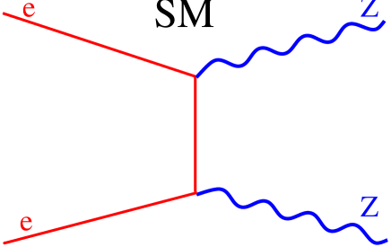
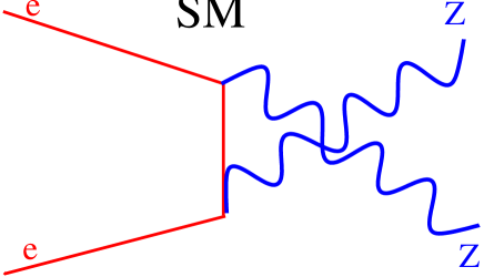
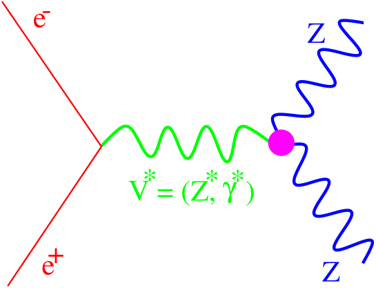
FIG. 1.: Diagrams contributing at first order to the $\mathrm{e^{+}e^{-}}\rightarrow\mathrm{Z}\mathrm{Z}$ process in the Standard Model.

FIG. 2.: Diagram with anomalous $\mathrm{Z}\mathrm{Z}\gamma$ and $\mathrm{Z}\mathrm{Z}\mathrm{Z}$ couplings contributing to the $\mathrm{e^{+}e^{-}}\rightarrow\mathrm{Z}\mathrm{Z}$ process.

FIG. 3.: Effect of non-standard couplings in the $\mathrm{e^{+}e^{-}}\rightarrow\mathrm{Z}\mathrm{Z}$ process at $\sqrt{s}=190~{}\mathrm{\ Ge\kern-1.00006ptV}$. A collision in the $\mathrm{e^{+}e^{-}}$ center-of-mass system is assumed. The angle $\theta_{Z}$ is the polar angle of one of the $\mathrm{Z}$ bosons and $d\sigma/d\cos\theta_{Z}$ is the differential cross section.

FIG. 4.: Effect of non-standard couplings in the $\mathrm{e^{+}e^{-}}\rightarrow\mathrm{Z}\mathrm{Z}$ process at $\sqrt{s}=500~{}\mathrm{\ Ge\kern-1.00006ptV}$. A collision in the $\mathrm{e^{+}e^{-}}$ center-of-mass system is assumed. The angle $\theta_{Z}$ is the polar angle of one of the $\mathrm{Z}$ bosons and $d\sigma/d\cos\theta_{Z}$ is the differential cross section.

FIG. 5.: Proportion of events in which both Z are longitudinally polarized (top left), both Z are polarized transversely (top right) or one is longitudinally and the other is transversely polarized (bottom) in a $\mathrm{e^{+}e^{-}}\rightarrow\mathrm{Z}\mathrm{Z}$ process at $\sqrt{s}=190~{}\mathrm{\ Ge\kern-1.00006ptV}$. Longitudinal and transverse polarizations are denoted by the labels “L” and “T”, respectively. Predictions for SM (continuous line) and anomalous $\mathrm{Z}\mathrm{Z}\mathrm{Z}$ couplings (dashed lines) are shown. A collision in the $\mathrm{e^{+}e^{-}}$ center-of-mass system is assumed. The angle $\theta_{Z}$ is the polar angle of one of the $\mathrm{Z}$ bosons.

FIG. 6.: Proportion of events in which both Z are longitudinally polarized (top left), both Z are polarized transversely (top right) or one is longitudinally and the other is transversely polarized (bottom) in a $\mathrm{e^{+}e^{-}}\rightarrow\mathrm{Z}\mathrm{Z}$ process at $\sqrt{s}=190~{}\mathrm{\ Ge\kern-1.00006ptV}$. Longitudinal and transverse polarizations are denoted by the labels “L” and “T”, respectively. Predictions for SM (continuous line) and anomalous $\mathrm{Z}\mathrm{Z}\gamma$ couplings (dashed lines) are shown. A collision in the $\mathrm{e^{+}e^{-}}$ center-of-mass system is assumed. The angle $\theta_{Z}$ is the polar angle of one of the $\mathrm{Z}$ bosons.

FIG. 7.: Proportion of events in which both Z are transversally polarized (left), or one is longitudinally and the other is transversely polarized (right) in a $\mathrm{e^{+}e^{-}}\rightarrow\mathrm{Z}\mathrm{Z}$ process at $\sqrt{s}=500~{}\mathrm{\ Ge\kern-1.00006ptV}$. Longitudinal and transverse polarizations are denoted by the labels “L” and “T”, respectively. The two figures at the top (bottom) illustrate the effect of possible anomalous $\mathrm{Z}\mathrm{Z}\mathrm{Z}$ ($\mathrm{Z}\mathrm{Z}\gamma$) couplings. The Standard Model predictions are shown with a continuous line, whereas the anomalous predictions are shown with dashed lines. A collision in the $\mathrm{e^{+}e^{-}}$ center-of-mass system is assumed. The angle $\theta_{Z}$ is the polar angle of one of the $\mathrm{Z}$ bosons. The case in which both Z are longitudinally polarized is not shown. It accounts for less than $0.5\%$ of the total.

FIG. 8.: Cross sections at $\sqrt{s}=190\mathrm{\ Ge\kern-1.00006ptV}$ for the different four-fermion channels taking into account all the diagrams (histogram) and only the neutral conversion ones (NC08). Some cuts (described in the text) have been applied in order to enhance the ZZ resonant contribution. Other diagrams are important when electrons, electronic neutrinos or fermions from the same isospin doublet are present in the final state.

FIG. 9.: Distributions of the relative difference, R, between the SM squared matrix elements computed by EXCALIBUR and by the NC08 approach. Only neutral conversion diagrams are taken into account. The plot a) shows the case of final states without identical fermions ($\mathrm{f}\bar{\mathrm{f}}\mathrm{f^{\prime}}\bar{\mathrm{f^{\prime}}}$). is shown in the plot. The plot b) contains those final states with identical fermions in the final state ($\mathrm{f}\bar{\mathrm{f}}\mathrm{f}\bar{\mathrm{f}}$). The effect of Fermi correlations (no effort has been done to include them in the NC08 approach) is visible as a tail in the distribution.

FIG. 10.: Distributions of the reweighting factor, W, in the $\mathrm{e^{+}e^{-}}\rightarrow\mathrm{Z}\mathrm{Z}(\gamma)\rightarrow\mathrm{f}\bar{\mathrm{f}}\mathrm{f^{\prime}}\bar{\mathrm{f^{\prime}}}(\gamma)$ process for different values of anomalous ZZV couplings. The reweighting factors are obtained with the FULL approach at $\sqrt{s}=190\mathrm{\ Ge\kern-1.00006ptV}$. Only neutral conversion diagrams are taking into account.

FIG. 11.: Distributions of the relative difference, R, between the weights computed with the FULL and the NC08 approaches. The process is $\mathrm{e^{+}e^{-}}\rightarrow\mathrm{Z}\mathrm{Z}(\gamma)\rightarrow\mathrm{f}\bar{\mathrm{f}}\mathrm{f^{\prime}}\bar{\mathrm{f^{\prime}}}(\gamma)$ at $\sqrt{s}=190\mathrm{\ Ge\kern-1.00006ptV}$ for different values of anomalous ZZV couplings. Only neutral conversion diagrams are taking into account.

FIG. 12.: Distributions of the optimal variable $O_{1}$ in the Standard Model (histogram) and in the presence of an anomalous coupling $f_{5}^{\mathrm{Z}}=0.01$ (points). The process under consideration is $\mathrm{e^{+}e^{-}}\rightarrow\mathrm{\ell^{+}\ell^{-}}\mathrm{q}\bar{\mathrm{q}}$ at $\sqrt{s}=500\mathrm{\ Ge\kern-1.00006ptV}$ and for an integrated luminosity of 100 fb^-1. The second plot shows the ratio between the anomalous and the SM distributions. A fit to the anomalous distribution leads to the value $f_{5}^{\mathrm{Z}}=0.010\pm 0.002$.

REFERENCES

• [1] CDF Collaboration, F.Β Abe etΒ al., Phys. Rev. Lett. 74 (1995) 1941;
DELPHI Collaboration, P.Β Abreu etΒ al.,
Phys. Lett. B 423 (1998) 194;
D0 Collaboration, B.Β Abbott etΒ al.,
Phys. Rev. D 57 (1998) 3817;
L3 Collaboration, M.Β Acciarri etΒ al.,
Phys. Lett. B 436 (1998) 187.
• [2] L3 Collaboration, M.Β Acciarri etΒ al., Phys. Lett. B 450 (1999) 281;
L3 Collaboration, M.Β Acciarri etΒ al.,
L3 Preprint 183, Submitted to Phys. Lett. B.
• [3] K.Β Hagiwara etΒ al., Nucl. Phys. B 282 (1987) 253–307.
• [4] β€œZ Physics at LEP1”, Ed. G.Β Altarelli etΒ al., CERN Yellow Book (1989), Vol 1, CERN 89-09, pag. 27.
• [5] D.Β Bardin, D.Β Lehner, T.Β Riemann, Nucl. Phys. B 477 (1996) 27.
• [6] T. SjΓΆstrand, CERN–TH/7112/93 (1993), revised August 1995;
T. SjΓΆstrand, Comp. Phys. Comm.Β  82 (1994) 74.
• [7] S.Β Jadach, W.Β Placzek, B.F.L.Β Ward, Phys. Rev. D 56 (1997) 6039.
• [8] J. Biebel, DESY 98-163;
A. Felbrich, private communication.
• [9] D.R.Β Yennie, S.Β Frautschi, H.Β Suura, Ann.Β Phys. 13 (1961) 379.
• [10] F.A. Berends, R. Kleiss and R. Pittau, Nucl. Phys. B 424 (1994) 308; Nucl. Phys. B 426 (1994) 344; Nucl. Phys. (Proc. Suppl.) B 37 (1994) 163;
R. Kleiss and R. Pittau, Comp. Phys. Comm. 83 (1994) 141;
R. Pittau, Phys. Lett. B 335 (1994) 490.