Partial Yukawa unification and a supersymmetric origin
of flavor mixing

Abstract

In a large class of supersymmetric SO(10) and left-right models, requiring that the effective theory below the scale of $SU(2)_{R}$ breaking be the MSSM implies partial Yukawa unification with $Y_{u}=Y_{d}$ and $Y_{e}=Y_{\nu^{D}}$. The same result also emerges in models with a horizontal $SU(3)_{H}$ symmetry. As a result, at the tree level, these models lead to vanishing quark mixing angles. We show that the correct mixing pattern can be generated in these models at the loop level from the flavor structure associated with the supersymmetry breaking terms. We generalize the constraints on supersymmetric parameters from flavor changing neutral current (FCNC) processes to include several squark mass insertions and confirm the consistency of the scheme. The expectations of this scheme for CP violating observables in the $B$ meson system are quiet different from the KM model, so it can be tested at the B factories.

I Introduction

One of the fundamental problems of the standard electroweak model is the lack of understanding of the fermion mass hierarchies and the flavor mixings. The minimal supersymmetric standard model (MSSM) which provides interesting resolution of the Higgs and the symmetry breaking puzzles does not shed any light on this question [1]. Supersymmetric grand unified theories do provide one framework within which question of flavor has been addressed in a variety of ways. While there are several interesting ideas, no particularly compelling model has emerged so far. It is worthwhile to pursue alternative approaches to the flavor problem. In this paper, we discuss one such approach.

We discuss two extensions of the MSSM which may provide an interesting new solution to the flavor question. At the tree level they lead to the equality of the up and the down type Yukawa matrices which we call up-down unification. While this class of models does not explain the microscopic origin of fermion mass hierarchies, the up-down unification implies that the quark mixing angles and the CP violating phase vanish at the tree level and arise purely as a result of radiative corrections. This would explain the smallness of these mixing parameters naturally. Flavor mixing associated with the soft supersymmetry breaking terms play a crucial role in inducing such mixings; we will show that they are compatible with existing flavor changing neutral current constraints (FCNC). We will argue that the required flavor structure arise quite naturally in a variety of supersymmetry breaking schemes.

One class of models which exhibits up-down unification is the supersymmetric left–right model with the seesaw mechanism[2] for small neutrino masses that has recently been discussed as a possible solution to the question of R-parity violation[3] and strong and weak CP violation problems of the MSSM[4]. The second class of models uses a horizontal $SU(3)_{H}$ symmetry (local or global). The latter belongs to the class of models which generically leads to relations between the masses of different generations of quarks. In our discussion however, we do not make the additional assumptions that lead to such mass relations, for example, specific pattern of VEVs for the Higgs fields. Rather, after we choose the Higgs sector, we allow them to have arbitrary VEVs and follow its consequences. It turns out that they then automatically lead to up-down unification in the sense we are going to discuss.

The main result that we wish to exploit in providing a radiative origin of quark mixings is the following. If we assume that below the new theory scale, i.e., the $SU(2)_{R}$ scale $v_{R}$ in the case of SUSYLR models and $SU(3)_{H}$ scale $v_{H}$ in the case of horizontal symmetry model, the theory is given by MSSM, then it is easy to show that there is up-down unification that leads to:

$$Y_{u} = Y_{d}$$ (1)

$$Y_{l} = Y_{\nu^{D}}~{}.$$ (2)

Strictly speaking, for the $SU(3)_{H}$ case, $Y_{u}=\beta_{q}Y_{d}$ and $Y_{l}=\beta_{l}Y_{\nu^{D}}$, where $\beta_{q,l}$ are ratios of two Yukawa couplings. But by redefining $\tan\beta\equiv\left\langle H_{u}\right\rangle/\left\langle H_{d}\right\rangle$ one can set $\beta_{q}=\beta_{l}=1$

While the up down unification is obvious in $SO(10)$ with a single 10 of Higgs representation, its generality when any number of 10’s and 126 Higgses are included was noted in Ref. [5]. This point was made in the context of SUSYLR model in Ref.[6]. To the best of our knowledge, the $SU(3)_{H}$ example has not been discussed before.

Eq. (1) implies that at the tree level, the quark mixing angles all vanish. We then show that consistent with the known constraints from flavor changing neutral currents and vacuum being charge and color preserving and stable, it is possible to generate desired values for the quark mixings. In this process we generalize existing constraints on the soft SUSY breaking terms from FCNC effects by allowing for several squark mass insertions and find that some may be relaxed.

This paper is organized as follows: in Sec. 2, we present the arguments leading to Eq. (1) in the supersymmetric left-right and the SO(10) models; in Sec. 3, we derive the same relations for the $SU(3)_{H}$ model. In Sec. 4, we outline our choice of soft supersymmetry breaking terms; in Sec. 5, we discuss the one loop graphs that induce the correct flavor mixings. In Sec. 6 we discuss the one loop effects from the off diagonal squark masses and the constraints on their magnitude from flavor changing neutral current effects; in Sec. 7, the same discussion is repeated for the off diagonal A-terms; and in Sec. 8 we discuss the origin of CP violation.

II Deriving Up-Down unification in the left-right and SO(10) models

In this section, we present a brief review of the arguments leading to the up-down unification in the SUSYLR model followed by its extension to the SO(10) model. We start by writing the superpotential of the SUSYLR model based on the gauge group$SU(2)_{L}\times SU(2)_{R}\times U(1)_{B-L}\times SU(3)_{c}$ (we have suppressed the generation index):

$$W = {\bf h}^{(i)}_{q}Q^{T}\tau_{2}\Phi_{i}\tau_{2}Q^{c}+{\bf h}^{(i)}_{l}L^{T}\tau_{2}\Phi_{i}\tau_{2}L^{c}$$ (3)

$$+ i({\bf f}L^{T}\tau_{2}\Delta L+{\bf f}_{c}{L^{c}}^{T}\tau_{2}\Delta^{c}L^{c})$$ (4)

$$+ M_{\Delta}{\rm Tr}(\Delta\bar{\Delta})+\Delta^{c}\bar{{\Delta}^{c}})+\lambda S(\Delta\overline{\Delta}-\Delta^{c}\overline{\Delta^{c}})+\mu_{S}S^{2}+\mu_{ij}{\rm Tr}(\tau_{2}\Phi^{T}_{i}\tau_{2}\Phi_{j})$$ (5)

$$+ W_{\it NR}~{}.$$ (6)

Here we use the standard notation (see Ref. [7]) where $Q,Q^{c}$ denote the left handed and right handed quark doublets, $L,L^{c}$ denote the lepton doublets, $\Phi_{i}$ are the (2,2,0,1) Higgs bi-doublets, $\Delta$ and $\Delta^{c}$ are the left and right handed Higgs triplets {(3,1,2,1) + (1,3,-2,1)} and $\bar{\Delta}$ and $\bar{\Delta^{c}}$ are fields conjugate to $\Delta,\Delta^{c}$. $W_{\it NR}$ denotes non-renormalizable terms arising from higher scale physics such as grand unified theories or Planck scale effects. The need for the nonrenormalizable term has been discussed in Ref.[7] and we do not repeat it here since it plays no role in our discussion.

We will work in the vacuum which conserves R-parity which implies that $v_{R}\geq 10^{10}$ GeV. In order to demonstrate the Yukawa unification, let us discuss the Higgs doublet spectrum of the model at low energies. Suppose that at the scale $v_{R}$, where $SU(2)_{R}$ breaks, we have an arbitrary number of bi-doublet fields $\Phi$’s. In order to get the MSSM at low energies, one must decouple all but one pair of $H_{u}$ and $H_{d}$ from the low energy spectrum. This has been called doublet-doublet splitting problem in literature. It is clear from the superpotential in Eq. (2) that doublet Higgsino matrix is symmetric because of parity invariance. For two bi-doublets for instance, it looks like:

$$M_{H}=\left(\begin{array}[]{cc}\mu_{11}&\mu_{12}\\ \mu_{12}&\mu_{22}\end{array}\right)~{}.$$ (9)

Eq. (3) is the mass matrix of bi-doublet $Higgsinos$, but since supersymmetry is broken at a much lower scale, the Higgs bosons will be degenerate with the Higgsinos. If we now do fine tuning to get one pair of $H_{u,d}$ at low energies, the $H_{u,d}$ appear as identical combinations of the doublets in $\Phi_{i}$’s. (Recall that a complex symmetric matrix may be diagonalized by the transformation $U^{T}M_{H}U=M_{H}^{\rm diag}$. This means that the rotations on $\Phi_{1}^{u}$ and $\Phi_{2}^{u}$ to get the MSSM $H_{u}$ is identical to the rotation on $\Phi_{1}^{d}$ and $\Phi_{2}^{d}$ to get $H_{d}$.) As a result, at the MSSM level, we have up down Yukawa unification, Eq. (1). It is clear that this result holds in the presence of arbitrary number of bi-doublet fields.

A similar situation appears in the case of a class of SUSY SO(10) models. Let us assume that the Higgs sector of the model has only 10 and $\overline{\bf 126}$’s and if there are 16-dimensional spinor fields, they do not participate in the low energy doublets (i.e., they do not mix with the 10 or $\overline{\bf 126}$). The main point here is that above the GUT scale there may be more than one pair of MSSM doublets contained in some 10 or in one of the $\overline{\bf 126}$. In order to get the MSSM below the GUT scale, one will have to diagonalize the doublet mass matrix so that one pair of light doublets remains light (doublet-doublet splitting). This may need a fine tuning of parameters, or it may appear naturally via the Dimopoulos-Wilczek mechanism [8]. We will not concern ourselves with its detail. Regardless of how many pairs of doublets couple to fermions at the GUT scale, as long as the doublet mass matrix is symmetric, the effective Yukawa couplings of the up and down sector Higgs ($H_{u}$ and $H_{d}$) of the MSSM are the same [5]. This leads to the afore-mentioned up-down unification[9]. Note that if the 16 and $\bar{\bf 16}$ fields participate in the low energy doublets, the $H_{u}$ and $H_{d}$ couplings are in general unrelated to each other[10].

There is one other class of SO(10) models where up-down unification of Eq. (1) would hold. Suppose there is a single 10 of Higgs that couples to fermions. In this case, even if the 16 spinors participates in electroweak symmetry breaking (by mixing with the 10), because there is only one Yukawa coupling matrix to begin with, Eq. (1) would hold. Note that in this case $\tan\beta$ is not restricted to be equal to $m_{t}^{0}/m_{b}^{0}$, this situation is analogous to the case of $SU(3)_{H}$ (see below).

III Horizontal symmetry and up-down unification

Let us now present a horizontal $SU(3)_{H}$ (local or global) model that leads to up-down unification. Consider MSSM$\otimes SU(3)_{H}$ as the high scale theory. Parity invariance is not necessary here. We assume that the matter multiplets of the MSSM transform as the 3 dimensional representation under the group [11]. Let us assume that we have Higgs doublet fields transforming as $\Phi_{u,d}(2,\pm 1,6^{*})$ under the gauge group $SU(2)_{L}\times U(1)_{Y}\times SU(3)_{H}$. Let us include an isosinglet field pair $S(1,1,6^{*})$ and ${\bar{S}}(1,1,6)$. The Horizontal symmetry is broken down at some high scale by the VEVs $\left\langle S\right\rangle=\left\langle\bar{S}\right\rangle=v_{H}X$ where $X$ is a symmetric $3\times 3$ matrix that does not commute with any of the SU(3) generators. The superpotential for the theory contains the following terms:

$$W_{H}=h_{u}Q\Phi_{u}u^{c}+h_{d}Q\Phi_{d}d^{c}+\Phi_{u}\Phi_{d}S+T(S\bar{S}-v^{2}_{H})~{},$$ (10)

where $T$ is a singlet used to break the $SU(3)_{H}$. In general one needs other fields such as $H-$octets etc to get the correct symmetry breaking pattern. There is no need for us to be explicit about them. It is clear from the superpotential that once $S$ field acquires arbitrary VEVs, we will get a symmetric $6\times 6$ mass matrix for the $\Phi_{u,d}$ fields. Since we want the MSSM to emerge at low energies, there will be some kind of fine tuning necessary at the $SU(3)_{H}$ scale. Due to the symmetry of the Higgs mass matrix, the MSSM Higgses $H_{u,d}$ will come out as the identical linear combination of the various $\Phi_{u,d}$ fields. This will then lead to the up-down unification Eq. (1) with $\beta_{q}=\frac{h_{d}}{h_{u}}$. A similar equation will also follow for the lepton sector. Even if there are an arbitrary number of $S$ fields, this result would hold. Note that $\tan\beta$ is a free parameter here, not restricted to be equal to $m_{t}^{0}/m_{b}^{0}$.

IV Nature of supersymmetry breaking terms

An immediate consequence of the above result (Eq. (1)) is that at the tree level the quark mixing angles vanish. However, once soft supersymmetry breaking terms are taken into account, they lead to correction to the tree level predictions via one loop diagrams. These diagrams not only correct the tree level mass spectrum bringing it more into agreement with observations but they also provide an explanation of the smallness of the CKM angles in a natural manner. In doing this, we will invoke two types of supersymmetry breaking terms: (i) The bilinear mass terms involving the superpartner fields, and (ii) the trilinear terms (the $A$ terms) that arise in generic supergravity and string models.

It would be necessary to have the generation changing bilinear terms to be much smaller than the generation diagonal bilinears in order to be compatible with known FCNC constraints. This type of a spectrum can be achieved in different scenarios of supersymmetry breaking: e.g. (1) dilaton dominated supersymmetry breaking [12], (2) anomalous $U(1)$ model[13], (3) models with nonabelian flavor symmetry[14], (4) gauge and gravity mediated supersymmetry breaking [15]. In all these models generational mixing bilinear terms are much suppressed (by a loop factor in (1), a chirality factor in (3) and a ratio of scales in (2) and (4)). The Kahler potential for these types of models can be written as:

$$K(z,z^{*};y_{i},y^{*}_{i})=M^{-2}_{Pl}(z^{*}z+y^{*}_{i}y_{i}+\epsilon_{ij}y^{*}_{i}y_{j})$$ (11)

where $\epsilon_{ij}$ are elements of a Hermiitian matrix, $y_{i}$ stand for the visible sector fields and $z$ is the hidden sector field. The $\epsilon_{ij}$ contributes to departures from universality for the soft scalar masses. The scalar masses can be written as follows:

$$m^{2}_{ij}=m^{2}_{0}(\delta_{ij}+\epsilon_{ij})~{}$$ (12)

with $\epsilon_{ij}\ll\delta_{ij}$.

If we use the trilinear $A$ terms for the generation of the quark (and lepton) mixing angles, the important requirement is that the generation dependence of the $A$ terms be different from the effective Yukawa couplings below the scale $v_{R}$. A significant point is that in the presence of a general Kahler potential there is no reason for the effective supersymmetry breaking mass or the $A$ terms surviving at the MSSM level to be proportional to the Yukawa couplings since the unitary matrices that diagonalize the Higgs mass matrix will not in general diagonalize the $A$ matrices. One can therefore write

$$A^{(a)}_{p,ij}=m_{1}Y^{(a)}_{p,ij}+m_{1}\epsilon_{ik}Y^{(a)}_{p,kj}~{}.$$ (13)

Here $m_{1}$ is a supersymmetry breaking mass parameter, the subscript $p$ stands for $u,d,l$ (quarks or leptons), and the superscript $(a)$ denotes the Yukawa coupling to the Higgs field $\Phi_{a}$. Below the $v_{R,H}$ scale, the diagonalization of the bilinear $\mu$ terms to get one pair of $H_{u},H_{d}$ diagonalizes only the first term in the above expression for $A$ and leaves the second term as arbitrary. Anticipating that FCNC effects require $\epsilon\ll 1$, we will then expect departures from the proportionality between $Y$ and $A$ to be of order $\epsilon$ without any extra strong suppressions due to $m_{q}/m_{W}$. The main reason for this is that we only expect one linear combination of the $v_{R}$ scale $Y_{p}$’s to lead to quark masses and the orthogonal one remains free. The $A$ term gets contributions from both the linear combination of $Y_{p}$’s. For example, in the SUSYLR model (Eq. (2)), suppose there are two bi-doublets $\Phi_{i}$. The MSSM doublet $H_{d}$ will be a linear combination $H_{d}=\cos\theta\Phi_{1}^{d}+\sin\theta\Phi_{2}^{d}$ (and similarly for $H_{u}$). If the angle $\theta$ is small, the Yukawa couplings $h^{(2)}_{q,ij}$ can be large, not proportional to the small quark masses. There could be other ways of generating departure from proportionality between the $A$ terms and the Yukawa couplings such as through the superpotentials as in models where the supersymmetry breaking is mediated by anomalous $U(1)$ gauge symmetries using more than one singlet.

In principle, both sources of flavor mixing will be present (Eqs, (6) and (7)). But for conceptual simplicity, we shall assume one among the two to be dominant. The results will change very little if both are combined. Furthermore, for most part, Eq. (6) and Eq. (7) lead to the same phenomenology as far as FCNC processes are concerned. One difference is in their cosmological implications. Color and charge breaking does restrict the nature of the trilinear $A$ terms, but not the bilinear terms, we shall discuss these in Sec. VII.

Although we begin with a parity–invariant theory in the cases of SUSYLR and SO(10) models, since $v_{R}$ will be assumed to be much larger than the SUSY breaking scale, the soft SUSY breaking parameters need not respect parity. Parity violation can show up in the soft breaking sector if they involve the VEV $v_{R}$ that breaks $SU(2)_{R}$. We will also discuss the possibility of maintaining parity invariance in the soft terms.

In the horizontal $SU(3)_{H}$ models, it is very natural to have the leading (renormalizable) term in the Kahler potential to be $SU(3)_{H}$ flavor symmetric. That would neatly resolve the SUSY flavor problem of supergravity models. $SU(3)_{H}$–violating terms can appear in the Kahler potential as higher dimensional terms involving standard model singlet fields suppressed by the Planck scale eg: $K\supset(M_{Pl}^{-4})(Q^{\dagger}Q)(S^{\dagger}S)$. If the VEVs of such $S$ fields are somewhat smaller than $M_{Pl}$, the smallness of $\epsilon_{ij}$ will be naturally explained.

V One loop contributions to quark masses and mixings

Let us restate the tree level mass relations predicted in these models. For simplicity, we focus on the SUSYLR or SO(10) type models:

$$M^{0}_{u} = \tan\beta M^{0}_{d}$$ (14)

$$M^{0}_{\nu^{D}} = \tan\beta M^{0}_{\ell}~{}.$$ (15)

It follows that both the quark mass matrices can be diagonalized by the same unitary matrix and hence the earlier assertion that $V_{CKM}={\bf 1}$. The same comment holds for the lepton sector too. Furthermore, since the Dirac masses for neutrinos are not known the second mass sum-rule involving the leptonic sector can help predict the neutrino masses. The mixing between different lepton generations would then arise from the see-saw formula which involves the Yukawa coupling of the $\Delta^{c}$ with off-diagonal elements (see the couplings ${\bf f}_{c}$ of Eq. (2)). That could potentially explain why the quark mixing angles are small (since they are induced at loop level), while the leptonic mixings are large (they already exist at the tree level). We will not discuss the leptonic mixing angles any further, we plan to return to this interesting question in a future paper. Here we will focus instead on the quark sector.

Before discussing quark mixings, let us first discuss the consistency of observed quark masses with the tree level predictions given in Eq. (8). Note that the above equation gives $\frac{m^{0}_{s}}{m^{0}_{c}}=\frac{m^{0}_{b}}{m^{0}_{t}}$ at the scale $v_{R}$. The superscript $0$ on the masses signify that they are the tree level masses evaluated at $\mu\sim M_{SUSY}$. Since $Y_{t}=Y_{b}$, when renormalization group extrapolated down to the weak scale, the relation is unchanged. Using the fact that at $\mu=M_{SUSY}\simeq m_{t}$, $m_{b}(\mu)\simeq 2.9$ GeV, $m_{t}\simeq 175$ GeV, $m_{c}(\mu)\simeq.67$ GeV and $m_{s}(\mu)\simeq.081$ GeV, the above relation among the tree level masses is seen to be off by almost a factor of eight. Clearly, large loop corrections must be invoked to resolve this discrepancy. Luckily, it has already been pointed out in the literature[16, 17] that in supergravity models (specially the ones with large $\tan\beta$), there are large radiative corrections to the bottom, strange and down quark masses arising through one–loop diagrams involving the exchange of gluino and the squarks (see Fig. 1). Analogous corrections to $m_{u},m_{c}$ and $m_{t}$ lack the $\tan\beta$ enhancement, so we focus on the corrections to $m_{d},m_{s}$ and $m_{b}$. There are two ways to resolve the above mass conundrum: (i) $b$–quark mass receives little correction from loops. In this case, $\tan\beta\simeq m_{t}^{0}/m_{b}^{0}\sim 60$ as in the SUSYLR model. Eq. (8) would then imply $m^{0}_{s}(\mu)\simeq.011$ GeV. The rest – actually the bulk – of the strange quark mass (about $.07$ GeV) can arise from the one loop gluino graph such as in Fig. 1. (ii) Loop corrections suppress the $b$–quark mass (Fig. 1 with all external quarks being $b$). This can happen for moderate values of $\tan\beta\simeq 10$. It will be consistent with one version of SO(10) model that was discussed (with one 10 of Higgs which mixes with 16), as well as the $SU(3)_{H}$ example. In this case the bulk of the strange quark mass comes from the tree level. $b$–quark mass receives large negative loop correction. There are two sources for $m_{b}$: the gluino–squark exchange and the chargino-stop exchange.

$$\delta m_{b}\simeq\frac{2\alpha_{s}}{3\pi}\frac{m_{\tilde{g}}}{m^{2}_{\tilde{q}}}(m_{b}^{0}\mu\tan\beta+A_{33}^{(d)}m_{0})+{\lambda_{t}^{2}\over 16\pi^{2}}{\mu\over m^{2}_{\tilde{q}}}(m_{b}^{0}\mu+A^{(u)}_{33}m_{0}\tan\beta)~{}.$$ (16)

In writing Eq. (9) we have assumed $m_{\tilde{q}}\gg m_{\tilde{g}},\mu$, but in our numerical estimate we use the exact expression. It might appear that the gluino exchange would lead to identical corrections for $\delta m_{b}/m_{b}$ and $\delta m_{s}/m_{s}$, but the trilinear $A_{33}^{(u),(d)}$ may not eqaul $A^{(u),(d)}_{22}$. Furthermore, the chargino contribution, which is comparable to the gluino contribution, is absent for the strange quark mass. We will discuss the numerical values of $m_{s}$ and $m_{b}$ after taking the loop correction into account in the next section after allowing for flavor mixing in the squark sector (which turns out to be significant for $m_{s}$).

As far as the first generation quarks go, if we choose the Yukawa coupling at the tree level such that $m_{u}\simeq.002~{}GeV$ (the right value) at $M_{SUSY}$, then we would get a tiny tree level value for $m_{d}$ . However, as is well known, the entire $m_{d}$ can arise in the process of generating flavor mixing angles. That is, $m_{d}\simeq\theta_{C}^{2}m_{s}$ works quite well. We will use this mechanism here to generate $m_{d}$. (This will require existence of both $\overline{d}_{L}s_{R}$ and $\overline{s}_{L}d_{R}$ terms in the down quark mass matrix. Only the former is needed for inducing $\theta_{C}$, see comments below.) Analogous expressions for $m_{s}$, viz., $m_{s}\simeq V_{cb}^{2}m_{b}$, is too small to explain the magnitude of $m_{s}$.

Let us now turn to the quark mixings. It is easier to induce off–diagonal elements in the down–quark mass matrix (rather than the up–quark matrix) for two reasons: (i) The one-loop diagram that would induce off–diagonal mixings have a $\tan\beta$ enhancement factor in the down sector but not in the up sector, and (ii) the charm and top quark masses are much larger in magnitude compared to the strange and bottom masses respectively, so the off–diagonal elements that are necessary in the up–quark mass matrix to generate the CKM mixings are larger (by about a factor of 10) compared to the ones needed in the down–quark sector. As we already noted, there are two ways to generate the off-diagonal terms in the quark mass matrices at the one loop level: (i) the off-diagonal terms in the bi-linear squark masses and (ii) the off-diagonal $A$ terms. In both cases we have to make sure that the magnitudes of the $A_{ij}$’s or $\Delta m^{2}_{ij}$’s needed are not in conflict with constraints of flavor changing neutral current effects [18]. We will see that there are parameter spaces where $A_{ij}$’s or $\Delta m^{2}_{ij}$ produce the required quark mixing without violating the bounds from the flavor changing neutral current. We now turn to address this important issue.

VI Quark mixings from off-diagonal squark masses

Here we will generalize the FCNC constraints arising from $K^{0}-\bar{K^{0}}$ system [18] to allow for several squark mass insertions that would be appropriate for our discussions. We will find that some of the constraints get relaxed because of the multiple insertions.

Let us first list the minimal number of mixing parameters among the generations we need in order to generate the quark mixings. These are determined as follows: The Cabibbo angle $V_{us}$ requires an effective entry $\overline{d}_{L}s_{R}$ in the down quark mass matrix. Similarly, $V_{cb}$ requires an entry $\overline{s}_{L}b_{R}$. Rather than using direct left–right squark mixings of the same flavor structure, we shall make use of the large $\tilde{b}_{L}-\tilde{b}_{R}$ mixing that is already present in the model. If in addition, we have $\tilde{d}_{L}-\tilde{b}_{L}$, $\tilde{b}_{L}-\tilde{s}_{L}$, and $\tilde{b}_{R}-\tilde{s}_{R}$, then effectively we can induce both $\overline{d}_{L}s_{R}$ and $\overline{s}_{L}b_{R}$ in the quark sector. For example, $\overline{d}_{L}s_{R}$ can arise via the chain $\tilde{d}_{L}-\tilde{b}_{L}\rightarrow\tilde{b}_{L}-\tilde{b}_{R}\rightarrow\tilde{b}_{R}-\tilde{s}_{R}$. Note that this set of parameters will also induce $V_{ub}$ via a $\overline{d}_{L}b_{R}$ quark mass term which arises from $\tilde{d}_{L}-\tilde{b}_{L}\rightarrow\tilde{b}_{L}-\tilde{b}_{R}$. We will discuss this constraint in detail, but let us note that in the process of inducing $V_{us}$ and $V_{cb}$, a non–zero value of $V_{ub}$ will already be induced given by $V_{ub}\simeq V_{us}V_{cb}$, which is roughly of the right order.

With this minimal set of SUSY flavor mixing parameters, we will generate adequate values of all CKM mixing angles. However, since the $\tilde{d}_{R}$ field does not appear in this minimal set, there will not be any significant correction to the $d$–quark mass. This deficiency will be removed when we later introduce an additional flavor mixing parameter $\tilde{d}_{R}-\tilde{b}_{R}$. We will show that $m_{d}\simeq\theta_{C}^{2}m_{s}$ will be induced in this case, without conflicting with the FCNC bounds. But at first we stick to the minimal set without $\tilde{d}_{R}-\tilde{b}_{R}$ mixing.

We will use $K^{0}-\bar{K}^{0}$ to constrain the mixing terms. This constraint turns out to be the most stringent. The only type of flavor changing operators generated by the above mixing terms are:

$$Q_{1} = \bar{d}^{\alpha}_{L}\gamma_{\mu}s^{\alpha}_{L}\bar{d}^{\beta}_{L}\gamma_{\mu}s^{\beta}_{L}\;,$$ (17)

$$Q_{2} = \bar{d}^{\alpha}_{L}s^{\alpha}_{R}\bar{d}^{\beta}_{L}s^{\beta}_{R}\;,$$ (18)

$$Q_{3} = \bar{d}^{\alpha}_{L}s^{\beta}_{R}\bar{d}^{\beta}_{L}s^{\alpha}_{R}\;.$$ (19)

The effective Hamiltonian involving these set of operators with different structure of the flavor changing bilinears is given in [18]. We write below the Hamiltonian, but after generalizing the loop functions to account for several squark mass insertions.

$$H = -\frac{\alpha_{s}^{2}}{216m_{\tilde{q}}^{2}}\Biggl{\{}\left(\delta^{d}_{12}\right)^{2}_{LL}\left(24\,Q_{1}\,x\,f_{6}(x)+66\,Q_{1}\,\tilde{f}_{6}(x)\right)$$ (20)

$$+ \left(\delta^{d}_{12}\right)^{2}_{LR}\left(204\,Q_{2}\,x\,f_{6}(x)-36\,Q_{3}\,x\,f_{6}(x)\right)\Biggr{\}}$$ (21)

where $x=m^{2}_{\tilde{g}}/m_{\tilde{q}}^{2}$, $m_{\tilde{q}}$ is the average squark mass, $m_{\tilde{g}}$ is the gluino mass, $(\delta^{d}_{ij})_{LL,LR}$ represent the product of mass insertions $\Delta m^{2}_{ij}/m^{2}_{\tilde{q}}$ that give rise to a particular operator and the functions $f_{6}(x)$ and $\tilde{f}_{6}(x)$ are given by :

$$f_{6}(x) = {1\over{60(x-1)^{7}}}(197+25x-300x^{2}+100x^{3}-25x^{4}+3x^{5}+60(1+5x)\ln x)~{},$$ (22)

$$\tilde{f}_{6}(x) = -{1\over{30(x-1)^{7}}}(-6-125x+80x^{2}+60x^{3}-10x^{4}+x^{5}-60x(1+2x)\ln x)~{}.$$ (23)

The diagrams for $K^{0}-\bar{K}^{0}$ mixing are shown in the Fig. 2. In Fig. 2a we use the mixing $\tilde{d}_{L}-\tilde{b}_{L}$, $\tilde{b}_{L}-\tilde{s}_{L}$ in both the squark lines. In Fig. 2b we use the mixing $\tilde{d}_{L}-\tilde{b}_{L}$, $\tilde{b}_{L}-\tilde{b}_{R}$ and $\tilde{b}_{R}-\tilde{s}_{R}$ in both the squark lines. We list the resulting constraints in Table 1 on the $\Re(\delta_{12})=\Re(\Delta m_{12}^{d^{2}}/m_{\tilde{q}}^{2})$ for an average squark mass $m_{\tilde{q}}=700~{}GeV$. We have used $m_{K}=498$ MeV, $f_{K}=160$ MeV and $m_{s}(1GeV)=150$ MeV as input.

$x$	$\sqrt{\left|\Re\left(\delta^{d}_{12}\right)_{LL}^{2}\right|}$	$\sqrt{\left|\Re\left(\delta^{d}_{12}\right)_{LR}^{2}\right|}$
0.1	$2.8\times 10^{-2}$	$7.5\times 10^{-3}$
0.3	$4.7\times 10^{-2}$	$8.0\times 10^{-3}$
2.0	$1.51\times 10^{-1}$	$1.2\times 10^{-2}$
4.0	$1.45\times 10^{-1}$	$1.5\times 10^{-2}$
8.0	$1.71\times 10^{-1}$	$2.0\times 10^{-2}$
10	$1.85\times 10^{-1}$	$2.2\times 10^{-2}$

Table 1: Upper limits on the product of squark mixings from $K^{0}-\bar{K^{0}}$ for an average squark mass $m_{\tilde{q}}=700\mbox{GeV}$ and for different values of $x=m_{\tilde{g}}^{2}/m_{\tilde{q}}^{2}$. For other values of $m_{\tilde{q}}$, the limits can be obtained by multiplying the ones in the table by $m_{\tilde{q}}(\mbox{GeV})/700$. $\Re$ stands for the real part. QCD corrections (not included in the Table) relax the bound in column 1 by about 30% and tighten it for column 2 by a factor of 2.

Using Table 1 and expressing $(\delta^{d}_{12})_{LL,LR}$ in terms of flavor changing mass insertions $\delta_{ij}$’s (where $\delta_{ij}=\Delta m^{2}_{ij}/m^{2}_{\tilde{q}}$, $\Delta m^{2}_{i,j}$ is the flavor mixing term), we can put bound on the mixing term $\delta_{d_{L}b_{L}}\delta_{b_{L}s_{L}}$ from column 1 and on the product $\delta_{d_{L}b_{L}}\delta_{b_{L}b_{R}}\delta_{b_{R}s_{R}}$ from column 2. Note that $\delta_{b_{L}b_{R}}$ can be obtained from our discussion of the loop correction to the $b$-quark mass. It is of order $\sim 1/10$ for $\tan\beta\simeq 25$ (since $\delta_{b_{L}b_{R}}={{m_{b}\mu\tan\beta}\over{m_{\tilde{q}}^{2}}}$ and if we choose $\mu=$600 GeV, $\tan\beta=25$, $m_{\tilde{q}}=700~{}GeV$ we get the above value). We can use this to put a bound on the term $\delta_{d_{L}b_{L}}\delta_{b_{R}s_{R}}$ from Table 1. It is important to note that the bounds obtained in Ref. [18] are relaxed in our case due to the particular flavor structure. We also find that the QCD correction [19] to $(LL)^{2}$ term increases the bound by $\sim 30\%$. For the $(LR)^{2}$, the upper bound tightens by a factor of 2.

The off diagonal elements in the quark mass matrices are generated at the one loop level via gluino-squark exchange. It is given by:

$$M_{23}=\frac{2\alpha_{s}}{3\pi}m_{\tilde{g}}\delta_{s_{L}b_{L}}\delta_{b_{L}b_{R}}f1_{M}~{},$$ (24)

$$M_{12}=\frac{2\alpha_{s}}{3\pi}m_{\tilde{g}}\delta_{d_{L}b_{L}}\delta_{b_{L}b_{R}}\delta_{s_{R}b_{R}}f2_{M}~{}.$$ (25)

The relevant diagrams are shown in Fig. 1. The loop functions that enter into the mass terms are given by:

$$f1_{M}={1\over{(1-x)^{2}}}(1-x+x\ln x)~{},$$ (26)

$$f2_{M}={1\over{2(1-x)^{3}}}(1-x^{2}+2x\ln x)~{}.$$ (27)

The functions are given in the limit where all the diagonal squark masses are equal. Since the mixing is small ($\sim 1/{10}$), using the same parameter space one finds that the functions with unequal masses differ from the above ones by less than 4$\%$.

The mixing angles $V_{cb}$ and $V_{us}$ arise from the down quark mass matrix elements $M_{23}$ and $M_{12}$ respectively. To generate the correct mixing angle for the quarks, they must have the values: $M_{23}\simeq V_{cb}m_{b}$ and $M_{12}\simeq V_{us}m_{s}$. Since the products of flavor changing transition entries for squarks are already constrained by the known bounds from FCNC processes in Table 1, we have to see if they allow us to generate the needed magnitudes of the $M_{ij}$. The $M_{23}$ element proves to be the most restrictive on the product of $\delta_{ij}$’s and once that is satisfied $M_{12}$ is automatically satisfied. In Table 2, we present the lower limits for the products of the $\delta_{ij}$’s required to generate the corresponding $M_{ij}$’s. (We use $V_{cb}=0.034$ and $V_{us}=0.22$.) In writing Table 2, we have assumed $m_{\tilde{q}}=700~{}GeV$.

$x$	$|\left(\delta^{d}_{M23}\right)_{LR}|$	$|\left(\delta^{d}_{M12}\right)_{LR}|$
0.1	$1.8\times 10^{-2}$	$6.2\times 10^{-3}$
0.3	$1.2\times 10^{-2}$	$4.7\times 10^{-3}$
2.0	$8.6\times 10^{-3}$	$4.4\times 10^{-3}$
4.0	$8.3\times 10^{-3}$	$4.9\times 10^{-3}$
8.0	$8.4\times 10^{-3}$	$5.7\times 10^{-3}$
10	$8.6\times 10^{-3}$	$6.2\times 10^{-3}$

Table 2: The lower limits on the products of $\delta_{ij}$’s required to generate the desired quark mixing angles (for $m_{\tilde{q}}=700~{}GeV$). The lower limits from column 2 should be compared with the upper limits from column 2 of Table 1 (divided by a factor of 2 for QCD correction). Compatibility is seen for $x\geq 0.3$.

We can now express $\left(\delta^{d}_{M12}\right)_{LR}\equiv\delta_{d_{L}b_{L}}\delta_{b_{L}b_{R}}\delta_{b_{R}s_{R}}$ and $\left(\delta^{d}_{M23}\right)_{LR}\equiv\delta_{s_{L}b_{L}}\delta_{b_{L}b_{R}}$. The upper limit on the first term can be read off from the second column of Table 1. Comparing with the lower limit from column 2 of Table 2, we find that the bound is well satisfied for $x>0.3$. Like before if the limit on the $\delta_{s_{L}b_{L}}$ is desired one should multiply the numbers in Table 2, first column by a factor ($\sim 10$) corresponding to $\tilde{b}_{L}-\tilde{b}_{R}$ mixing.

There are two contributions to $V_{ub}$, one goes as the product $V_{us}V_{cb}$ and the other is $M_{13}/m_{b}$. Here $M_{13}$ is the loop contribution to the (1,3) entry of the down quark mass matrix arising from a diagram analogous to Fig. 1b (replace $s_{L}$ by $d_{L}$ in Fig. 1b). The estimate of $M_{13}$ is obtained from Eq. (13) by the replacement $\delta_{s_{L}b_{L}}\rightarrow\delta_{d_{L}b_{L}}$. Using the relation $V_{ub}=V_{us}V_{cb}+M_{13}/m_{b}$, setting its magnitude equal to $0.006$, and allowing for the two contributions to have a relative negative sign, we find that $|M_{13}|\leq 0.045~{}GeV$. For $m_{\tilde{q}}=700~{}GeV$ and $x=0.1$, this corresponds to the limit $\delta_{d_{L}b_{L}}\delta_{b_{L}b_{R}}\leq 0.012$. On the other hand, from the required value of $V_{us}$, we have a lower limit (for the same set of parameters) $\delta_{d_{L}b_{L}}\delta_{b_{L}b_{R}}\delta_{b_{R}s_{R}}\geq 6.2\times 10^{-3}$ (see Table 2). Comparing the two constraints, we find that $\delta_{b_{R}s_{R}}\geq 0.5$ . Thus there is large mixing in the $\tilde{b}_{R}-\tilde{s}_{R}$ sector, but that is consistent with all phenomenological constraints.

The process $b\rightarrow s\gamma$ does provide some useful limits. There is a diagram similar to Fig. 1b with $s_{L}$ replaced by $s_{R}$ and the squark line emitting a photon. From Ref. [18], $b\rightarrow s\gamma$ puts a limit on the product $\delta_{b_{R}s_{R}}\delta_{b_{L}b_{R}}\leq 1.3\times 10^{-2}(m_{\tilde{q}}/500~{}GeV)^{2}$. For a squark mass of 1 TeV and for $\delta_{b_{R}s_{R}}\simeq 0.5$, we see that $\delta_{b_{L}b_{R}}$ should be less than about $0.1$. This would seem to prefer the scenario with moderate $\tan\beta$, although the large $\tan\beta$ scenario is not inconsistent if $\mu$ is much smaller than the squark masses.

As for the diagonal strange quark mass, it arises from a diagram analogous to Fig. 1b. The magnitude is given by Eq. (14) with $\delta_{d_{L}b_{L}}$ replaced by $\delta_{s_{L}b_{L}}$. We will now show that this is just of the right order needed.

Let us choose a definite set of numbers to check the self–consistency of the scheme. Let $m_{\tilde{q}}=700~{}GeV$ and $m_{\tilde{g}}\simeq 400~{}GeV$, so that $x\simeq 0.3$. We also choose, for this example, $\delta_{b_{L}b_{R}}=0.1$. The shift in $b$–quark mass from the gluino graph alone is then $\Delta m_{b}=0.7~{}GeV$, which is small. Including the chargino diagram, this shift may even be smaller. Next consider $V_{cb}\simeq M_{23}/m_{b}$. Setting it equal to $0.034$ determines $\delta_{s_{L}b_{L}}\simeq 0.15$. Setting the diagonal mass of the strange quark arising from the gluino exchange equal to $0.03~{}GeV$, we get $\delta_{s_{R}b_{R}}\simeq 0.65$. Next we set $|V_{ub}|=|V_{us}V_{cb}-M_{13}/m_{b}|$ equal to $0.006$. With a relative negative sign between the two terms, we find $\delta_{d_{L}b_{L}}\simeq 0.065$. This choice will now determine $V_{us}\simeq M_{12}/m_{s}$, since there are no more parameters. We find it is given by $V_{us}\simeq(11~{}MeV/m_{s})$, where $m_{s}$ is the $full$ strange quark mass at $\mu\sim 175~{}GeV$. This is of the right size for $m_{s}(\mu\sim 175~{}GeV)\simeq 0.05~{}GeV$ (corresponds to $m_{s}(1~{}GeV)\simeq 0.133~{}GeV$). This shows the consistency of the scenario.

So far in the flavor mixings of the squarks, we have not assumed left-right symmetry. If we however demand left right symmetry is preserved by the soft supersymmetry breaking terms, we will have an additional mixing term $\tilde{d}_{R}-\tilde{b}_{R}$. Such a mixing entry will also enable us to induce acceptable $d$–quark mass. The strength of various operators would be related by parity invariance. The new operators induced by this new term are:

$$\tilde{Q}_{1}: Q_{1}({\rm L\leftrightarrow R}),$$ (28)

$$\tilde{Q}_{2}: Q_{2}({\rm L\leftrightarrow R}),$$ (29)

$$\tilde{Q}_{3}: Q_{3}({\rm L\leftrightarrow R}),$$ (30)

$$Q_{4} = \bar{d}^{\alpha}_{R}s^{\alpha}_{L}\bar{d}^{\beta}_{L}s^{\beta}_{R},$$ (31)

$$\tilde{Q}_{4}: Q_{4}({\rm L\leftrightarrow R}),$$ (32)

$$Q_{5} = \bar{d}^{\alpha}_{R}s^{\beta}_{L}\bar{d}^{\alpha}_{L}s^{\beta}_{R},$$ (33)

$$\tilde{Q}_{5}: Q_{5}({\rm L\leftrightarrow R}).$$ (34)

These new operators will introduce new terms in the Hamiltonian:

$$H_{\rm extra} = -\frac{\alpha_{s}^{2}}{216m_{\tilde{q}}^{2}}\Biggl{\{}\left(\delta^{d}_{12}\right)^{2}_{RR}\left(24\,\tilde{Q}_{1}\,x\,f_{6}(x)+66\,\tilde{Q}_{1}\,\tilde{f}_{6}(x)\right)$$ (36)

$$+ \left(\delta^{d}_{12}\right)_{LL}\left(\delta^{d}_{12}\right)_{RR}\left(504\,Q_{4}\,x\,f_{6}(x)-72\,Q_{4}\,\tilde{f}_{6}(x)\right.$$ (37)

$$+ \left.24\,Q_{5}\,x\,f_{6}(x)+120\,Q_{5}\,\tilde{f}_{6}(x)\right)$$ (38)

$$+ \left(\delta^{d}_{12}\right)^{2}_{RL}\left(204\,\tilde{Q}_{2}\,x\,f_{6}(x)-36\,\tilde{Q}_{3}\,x\,f_{6}(x)\right)$$ (39)

$$+ \left(\delta^{d}_{12}\right)_{LR}\left(\delta^{d}_{12}\right)_{RL}\left(-132\,Q_{4}\,\tilde{f}_{6}(x)-180\,Q_{5}\,\tilde{f}_{6}(x)\right)\Biggr{\}}~{}.$$ (40)

The LLRR diagram can appear without a LR mixing now, i.e., $\tilde{d}_{L}-\tilde{b}_{L}$ and $\tilde{b}_{L}-\tilde{s}_{L}$ on one line of the box diagram and $\tilde{d}_{R}-\tilde{b}_{R}$ and $\tilde{b}_{R}-\tilde{s}_{R}$ on the other line of the same diagram. The upper bound on the $\left(\delta^{d}_{12}\right)_{LL}\left(\delta^{d}_{12}\right)_{RR}$ term is shown in Table 3.

$x$	$\sqrt{\left|\Re\left(\delta^{d}_{12}\right)_{LL}\left(\delta^{d}_{12}\right)_{RR}\right|}$
0.1	$4.0\times 10^{-3}$
0.3	$4.3\times 10^{-3}$
2.0	$6.6\times 10^{-3}$
4.0	$8.5\times 10^{-3}$
8.0	$1.1\times 10^{-2}$
10	$1.3\times 10^{-2}$

Table 3: Upper limits on the products of $\delta$’s obtained for an average squark mass $m_{\tilde{q}}=700~{}\mbox{GeV}$ and for different values of $x=m_{\tilde{g}}^{2}/m_{\tilde{q}}^{2}$. For other values of $m_{\tilde{q}}$, the limits can be obtained by multiplying the ones in the Table by $m_{\tilde{q}}(\mbox{GeV})/700$.

Before we discuss the consequences of Table 3, let us comment on the generation of $d$–quark mass purely from mixing with $s$ and $b$. Clearly, that requires the $\tilde{d}_{R}-\tilde{b}_{R}$ mixing term. There are two contributions to the $d$ mass, one from mixing with the $b$ and the other from mixing with the $s$. The former has a magnitude $\sim V_{ub}^{2}m_{b}$, while the latter goes as $V_{us}^{2}m_{s}$. Numerically the contribution from $d-s$ mixing is more important and of the right magnitude. So we focus on it. For this estimate to hold, the $\overline{s}_{L}d_{R}$ entry in the down quark mass matrix should have the same magnitude as the $\overline{d}_{L}s_{R}$ entry. The lower limit on the mixing parameters obtained by demanding that $M_{21}^{d}\geq\theta_{C}m_{s}$ are the same as in Table 2, second column. (One can simply replace $L\rightarrow R$ in Eq. (14) to get $M_{21}$. All the relevant loop functions are the same.) Similarly, the upper limits from FCNC on $\Re(\delta_{21}^{d})_{LR}$ are identical to the numbers listed in Table 1, column 2. This is because of the parity inavariance respected by the gluino box diagram. We see that there is broad agreement between the two sets of numbers, implying that reasonable $d$–quark mass can be induced by pure mixing.

From Table 3 we find the upper limit on the mixing term $\sqrt{\delta_{d_{L}b_{L}}\delta_{b_{L}s_{L}}\delta_{d_{R}b_{R}}\delta_{b_{R}s_{R}}}$. Assuming $\delta_{d_{L}b_{L}}\delta_{b_{L}s_{L}}=\delta_{d_{R}b_{R}}\delta_{b_{R}s_{R}}$, we can use the bounds shown in Table 3 to put upper limit on $\delta_{d_{L}b_{L}}\delta_{b_{L}s_{L}}$. On the other hand, Table 2 gives the lower limit on $\delta_{d_{L}b_{L}}\delta_{b_{L}s_{L}}\delta_{b_{L}b_{R}}$. If $\delta_{b_{L}b_{R}}$ is $\sim 1/10$, the lower limit surpasses the upper limit when multiplied by this factor of 10. Thus, for the choice of parameters we have made, it is not possible to maintain left-right symmetry in the soft SUSY breaking terms. This is not a disaster for the model since there may be hidden sector effects which may be able to generate the necessary left-right breaking effects in the soft SUSY breaking sector. This is especially so if the scale of $SU(2)_{R}$ breaking is higher than that of supersymmetry breaking. Another possibility is to use a different choice of parameter space where $\delta_{b_{L}b_{R}}$ $\sim 1$ so that bounds in the Table 3 do not contradict the assumption of left-right symmetry. This choice, for example, would correspond to large $\tan\beta\sim 60$, with $\mu\sim 1~{}TeV$ ($m_{0}=450$ GeV and $m_{\tilde{g}}=1.5$ TeV). Such a large value of $\mu$ will require some fine tuning to obtain the Z-mass consistent with radiative electroweak symmetry breaking, but is perhaps not out of question.

Other FCNC processes, such as from the loop induced $dsZ$ vertex or $ds$-Higgs vertex, satisfy all the phenomenological constraints, mainly due to the decoupling behavior of supersymmetric theories.

VII Quark mixings from off-diagonal A terms

The elements $M_{12}$ and $M_{23}$ can also be generated from the off diagonal A terms. Again let us take a minimal flavor mixing structure. We assume that $A_{23}$ gives rise to $\tilde{s}_{L}\tilde{b}_{R}$ mixing and $A_{12}$ gives rise to $\tilde{d}_{L}\tilde{s}_{R}$ mixing. If left–right symmetry is preserved, we need two more $A$’s induce $\tilde{b}_{L}\tilde{s}_{R}$ and $\tilde{s}_{L}\tilde{d}_{R}$ terms ($A_{21}$ and $A_{32}$ respectively). We shall assume $A_{23}=A_{32}~{}{\rm and}A_{12}=A_{21}$ in this case. We also have a $\tilde{b}_{L}\tilde{b}_{R}$ term induced by the $\mu\tan\beta$ term as before.

The FCNC bound on $A_{12}$ can be obtained from the $K^{0}\bar{K^{0}}$. The diagram will look like the fig. 1 with one cross on each squark line, where the cross represents the A term. The functions needed to calculate this diagram are given in the Ref. [18]. We find, for $m_{\tilde{q}}$=600 GeV and $m_{\tilde{g}}=1$ TeV, $A_{12}v_{d}/m_{\tilde{q}}^{2}$ has to be less than $7\times 10^{-3}$. For the same parameter space, the lower bound on the $A_{12}v_{d}/m_{\tilde{q}}^{2}$ is $1\times 10^{-3}$ from the one loop $\overline{d}_{L}s_{R}$ mass diagram involving gluino and squarks. The squark line will now have the $\tilde{d}_{L}\tilde{s}_{R}$ mixing term arising from $A_{12}$ (see Fig. 1). The function $f1_{M}$ is used for this calculation.

The $\overline{s}_{L}b_{R}$ mixing diagram will be generated by gluino mediation and in the squark line the off–diagonal $A_{s_{L}b_{R}}$ appears. For $m_{\tilde{q}}$=600 GeV and $m_{\tilde{g}}=1$ TeV we find the bound on the $A_{23}v_{d}/m_{\tilde{q}}^{2}\geq 0.009$ from the mass diagram. There is no significant upper bound on $A_{b_{L}s_{R}}$ term from the available data. Hence we will have a viable solution with left right symmetry intact.

Unlike the case of bi-linear mass terms, there could be two other indirect bounds for the case of tri-linear $A$ terms. These are the color and charge breaking bounds (CCB) and unbounded from below (UFB) bound [20]. If these bounds are violated, the true vacuum of the MSSM may be either unstable or it may be color and charge breaking. These indirect bounds are not on the same footing as the FCNC bounds which are very direct. It is not clear whether the CCB and UFB bounds are absolute bounds, they may be evaded in various early universe scenarios [21], for example if our universe is in a metastable vacuum and if the tunneling rate to the true vacuum is much slower than the age of the universe. They may also be evaded if non–renormalizable terms in the potential are taken into account or equivalently, if the theory gives in to a new theory at a higher energy scale. For completeness we list these CCB and UFB bounds below.

The most stringent (for our purpose) CCB bound is given as [20]:

$$|A^{(d)}_{ij}|\leq\lambda^{2}_{dk}(m^{2}_{d_{L_{i}}}+m^{2}_{d_{R_{i}}}+m^{2}_{d_{1}}),~{}k=Max(i,j)$$ (41)

where $m_{1}^{2}=m_{H_{2}}^{2}+\mu^{2}$. The UFB bound is given as [20]:

$$|A^{(d)}_{ij}|\leq\lambda^{2}_{dk}(m^{2}_{d_{L_{i}}}+m^{2}_{d_{R_{i}}}+m^{2}_{d_{\nu_{m}}}),~{}k=Max(i,j)~{}.$$ (42)

The UFB and CCB bound requires $A_{23}v_{d}/m_{\tilde{q}}^{2}\leq 0.009$. Hence we have a viable $A_{23}$ mixing. However $A_{12}$ term is a problem. From the UFB and CCB bound we have $A_{12}v_{d}/m_{\tilde{q}}^{2}\leq 0.0002$, which is smaller than the lower limit required for generating $V_{us}$. The problem with this $A_{12}$ term happens because the UFB or the CCB bound on this term involves the $s$-quark coupling. The CCB bound involves $m^{2}_{\nu_{m}}$ and the UFB bound involves $m_{1}^{2}(=m_{H_{1}}^{2}+\mu^{2})$. So if we make $m^{2}_{\nu_{m}}$ or $m_{H_{1}}^{2}$ larger, it is possible to have a viable $A_{1,2}$ mixing. FCNC constraint can be satisfied in both the cases, although with a heavy supersymmetric spectrum.

In the left-right model leading to MSSM at low energies, these constraints need not apply for the following reason: If we are working at the $SU(2)_{L}\times SU(2)_{R}\times U(1)_{B-L}\times SU(3)_{c}$ level, it has been shown that below the scale $v_{R}$, in addition to the interactions of MSSM, there is an additional interaction of the form $W_{extra}=f_{ij}e^{c}_{i}e^{c}_{j}{\Delta^{c}}^{--}$ [7]. This gives new quartic terms to the potential that invalidate the CCB bounds of MSSM in the lepton sector. If we extend the gauge group to $SU(2)_{L}\times SU(2)_{R}\times SU(4)_{c}$, there can be analogous interactions involving quarks which can help avoid the CCB bounds in the quark sector. Also in this class of models, above $10^{10}$ GeV a new theory takes over which can substantially alter the vacuum structure.

Let us now point out that while we have conducted the discussion of the sections V-VII within the framework of the SO(10) or SUSYLR type models, they are applicable to the $SU(3)_{H}$ models without any modification. The only point worth noting here is that the presence of the horizontal symmetry at a high scale implies that the soft breaking terms must originate from basic interactions that are $SU(3)_{H}$ invariant after horizontal symmetry breaking. Such a situation can always be arranged by including extra $SU(3)_{H}$ multiplets (such as an $H$–octet) which do not couple to matter fields and giving them appropriate VEVs. We do not elaborate on these points since they involve standard methods.

VIII CP violation

The simplest way to introduce CP violation into this model is by assuming that the flavor mixing parameters $\epsilon_{ij}$ in Eqs. (6)-(7) are complex. In Tables 1 and 3 we listed the lower limits on the flavor mixing parameters arising from the real part of the $K^{0}-\bar{K^{0}}$ amplitude. There are constraints from the imaginary part too, they are more stringent by about a factor of 200 compared to the numbers in Tables 1 and 3. This suggests that if the relevant phases that enter into the gluino box diagram (see Fig. 2) are of order $3\times 10^{-3}$, these gluino box diagrams themselves can explain the observed value of $\epsilon$ in the $K$ meson system. Note that if the phases of $\epsilon_{ij}$ are of order $3\times 10^{-3}$, the KM phase will be too small to account for $\epsilon_{K}$. This has implications for the B system.

If CP violation occurs only in the mixing, it might be though that this is a superweak model of CP violation. But it is actually not. The direct CP violating parameter $\epsilon^{\prime}/\epsilon$, receives a one-loop contribution from the gluino penguin graph. This diagram has been calculated in Ref. [22], and that result can be directly applied to the model we are discussing. It was shown in Ref. [22] that $\epsilon^{\prime}/\epsilon=$ ( 1 to 3)$\times 10^{-3}$ (modulo hadronic uncertainty). The reason for such a relatively large value has to do with the chiral structure associated with the gluino penguin graph of these models.

Thus there is “approximate CP invariance” [23] in this class of models. This means that all the phases are small, of order $10^{-2}$, including the phases of the gluino mass, $\mu$ parameter and $A$ and $B$ terms. This is a welcome result since it can explain the smallness of neutron and electron electric dipole moments, which is otherwise a puzzle in supersymmetric models. With all phases being order $10^{-2}$, EDM of electron and neutron become consistent with experiment. (We assume that the contribution to the neutron EDM from the strong CP phase is rendered harmless either by the axion solution or by the constraints of left-right symmetry[4].) KM model of CP violation is not operative here. This is especially significant for CP asymmetries in the $B$ meson system. In the KM model, many of the asymmetries are large, of order 10% or larger. In our scenario, all asymmetries in the $B$ system are expected to be too small. The reason being the smallness of all CP violating parameters. (Recall that the phase in the KM model is not small.) If at the B factory, CP asymmetries are measured to be large, that could exclude this scenario.

IX Conclusion

To summarize, we have discussed how the partial Yukawa unification that results in a large class of SO(10) and SUSY left-right models as well as a class of horizontal symmetry models provides a new way to understand the smallness of quark mixing angles. Generating the appropriate flavor mixings requires a specific pattern for the soft breakings. As is well known, there are strong constraints on the allowed pattern of soft breakings from flavor changing neutral current effects. We have shown by a detailed analysis how the pattern needed for our purpose is consistent with the constraints of FCNC effects. They are also compatible with constraints arising by demanding that the vacuum be bounded from below and that it conserves color and electric charge.

One place where this class of models may be subjected to experimental scrutiny is CP violating asymmetries in the $B$ meson system which will be measured at the B factories. Unlike the KM model, all CP asymmetries in the $B$ system are predicted to be too small, by the requirement of approximate CP invariance. These models predict neutron and electron EDM near the present experimental limits. A third crucial test of the model involves the branching ratios of the Higgs into fermion pairs. Since the mass relation $m_{s}^{0}/m_{b}^{0}=m_{c}^{0}/m_{t}^{0}$ is corrected by suppressing $m_{b}^{0}$ via the one loop gluino contribution in one scenario, the higgs branching ratio $\Gamma(h\rightarrow b\overline{b})/\Gamma(h\rightarrow\tau^{+}\tau^{-})$ will differ significantly from its standard model value [24]. The same diagrams that contribute to off–diagonal quark and lepton mixings can lead to flavor violating Higgs decays. Decays of the Higgs into lepton pairs $h\rightarrow l_{i}^{+}l_{j}^{-}$ for $i\neq j$ would provide dramatic signatures in support of this class of models. To have an observable event rate, however, one would have wait for a Higgs factory such as the muon collider. In contrast to Ref. [25], in our scheme the diagonal muon mass arises already at the tree level, so no large effect is expected in the $g-2$ of the muon.

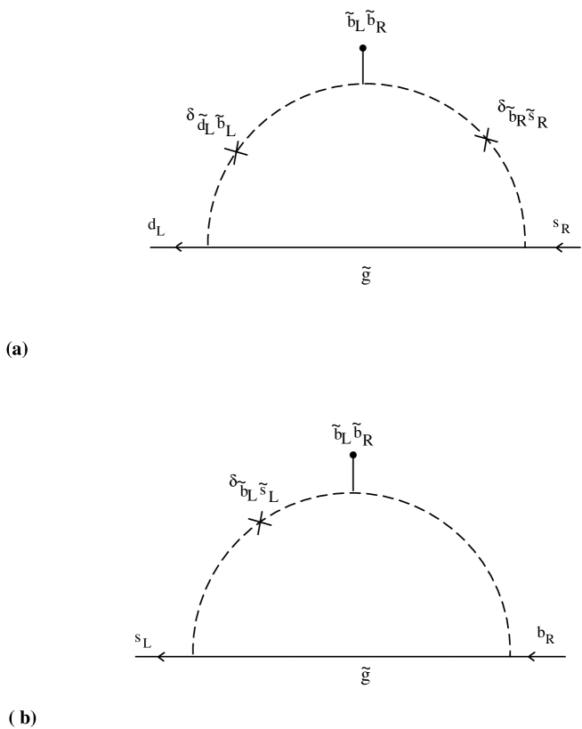
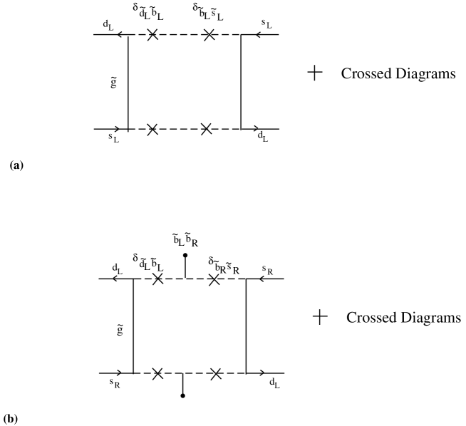
FIG. 1.: Gluino-squark diagrams for the generation of down quark masses and CKM angles.

FIG. 2.: SUSY contributions to the $K^{0}-\bar{K}^{0}$ process.

REFERENCES

- [1] For a recent review of the MSSM and its problems, see S. Martin, hep-ph/9709356; K. Dienes and C. Kolda, hep-ph/9712322; to appear in Perspectives in Supersymmetry, ed. G. Kane, World Scientific, 1998.
- [2] M. Gell-Mann, P. Ramond and R. Slansky, in Supergravity ed. D. Freedman et al. (North Holland, 1979); T. Yanagida, KEK Lectures (1979); R. N. Mohapatra and G. Senjanović, Phys. Rev. Lett. 44, 912 (1980).
- [3] R. N. Mohapatra, Phys. Rev. D34, 3457 (1986); A. Font, L. Ibanez and F. Quevedo, Phys. Lett. B228, 79 (1989); S. Martin, Phys. Rev. D 46 , 2769 (1992).
- [4] R. N. Mohapatra and A. Rasin, Phys. Rev. Lett. 76, 3490 (1996); R. Kuchimanchi, Phys. Rev. Lett. 76, 3486 (1996); R. N. Mohapatra , A. Rasin and G. Senjanović, Phys. Rev. Lett. 79, 4744 (1997).
- [5] D. G. Lee and R. N. Mohapatra, Phys. Rev. D51, 1353 (1995).
- [6] C. Aulakh, A. Melfo, A. Rasin and G. Senjanović, hep-ph/9712551.
- [7] R. Kuchimanchi and R. N. Mohapatra, Phys. Rev. D48, 4352 (1993); Phys. Rev. Lett. 75, 3989 (1995); Z. Chacko and R. N. Mohapatra, hep-ph/9712359; Phys. Rev. D 58, 015001 (1998); C. Aulakh, A. Melfo and G. Senjanović, hep-ph/9707258.
- [8] S. Dimopoulos and F. Wilczek, Report No. NSF-ITP-82-07 (1981), in The unity of fundamental interactions, Proc. of the 19th Course of the International School of Subnuclear Physics, Erice, Italy, 1981, Plenum Press, New York (ed. A. Zichichi); K.S. Babu and S.M. Barr, Phys. Rev. D48, 5354 (1993).
- [9] For discussions of up-down unification in other models, see D. Chang, R. N. Mohapatra, P. B. Pal and J. C. Pati, Phys. Rev. Lett. 55, 2756 (1985); C. Hamzaoui and M. Pospelov, hep-ph/9803354.
- [10] K. S. Babu and R. N. Mohapatra, Phys. Rev. Lett. 74, 2418 (1995); K.S. Babu and S.M. Barr, Phys. Rev. D56, 2614 (1997); S.M. Barr and S. Raby, Phys. Rev. Lett 79, 4748 (1997); C. Albright and S. Barr, hep-ph/9712488; Z. Chacko and R. N. Mohapatra, hep-ph/9808458; hep-ph/9810315.
- [11] See for example, Z. Berezhiani, Phys. Lett. B417, 287 (1998).
- [12] J. A. Casas, hep-ph/9605180 and references therein.
- [13] P. Binetruy and E. Dudas, Phys. Lett. B389, 503 (1996); G. Dvali and A. Pomarol, Phys. Rev. Lett. 77, 3728 (1996); R. N. Mohapatra and A. Riotto, Phys. Rev. D 58, 1138 (1997); A. Farragi and J. C. Pati, Nucl. Phys. B 526, 18 (1998).
- [14] A. Pomarol and D. Tommasini, Nucl. Phys. B 466, 3 (1996); R. Barbieri, L. Hall and A. Romanino, Phys. Lett. B 401, 47 (1998).
- [15] N. Arkani-Hamed, J. March-Russell and H. Murayama, Nucl. Phys. B509, 3 (1998).
- [16] L. Hall, R. Rattazi and U. Sarid, LBL-33997 (1993); T. Blazek, S. Pokorski and S. Raby, hep-ph/9504364.
- [17] For models which use the gluino graph to generate quark masses, see: T. Banks, Nucl. Phys. B303, 172 (1988); E. Ma, Phys. Rev. D39, 1922 (1989); R. Hempfling, Phys. Rev. D49, 6168 (1994).
- [18] F. Gabbiani, E. Gabrielli, A. Masiero, M. Silvestrini, Nucl. Phys. B477, 321 (1996); L. J. Hall, V. A. Kostelecky and S. Raby, Nucl. Phys. B267, 415 (1986).
- [19] J. Bagger, K. Matchev and R. Zhang, hep-ph/9707225.
- [20] S. Dimopoulos and J. A. Casas, hep-ph/9606237.
- [21] A. Kusenko, P. Langacker and G. Segre, Phys. Rev. D 54, 5824 (1996).
- [22] K.S. Babu and S.M. Barr, Phys. Rev. Lett. 72, 2831 (1994).
- [23] G. Eyal and Y. Nir, Nucl. Phys. B528, 21 (1998).
- [24] K.S. Babu and C. Kolda, hep-ph/9811308.
- [25] F.M. Borzumati, G. Farrar, N. Polonsky and S. Thomas, hep-ph/9712428.