Topological Defects in the Left-Right Symmetric Model and their Relevance to Cosmology

Abstract

It is shown that the minimal left-right symmetric model admits cosmic string and domain wall solutions. The cosmic strings arise when the $SU(2)_{R}$ is broken and can either be destabilized at the electroweak scale or remain stable through the subsequent breakdown to $U(1)_{EM}$. The strings carry zero modes of the neutrino fields. Two distinct domain wall configurations exist above the electroweak phase transition and disappear after that. Their destabilization provides new sources of non-equilibrium effects below the electroweak scale which is relevant to baryogenesis.

I. INTRODUCTION

Topological defects are regions of trapped energy density which can be produced at the time of cosmological phase transitions and survive after that if the topology of the vacuum manifold of the theory is nontrivial. Typically, cosmological phase transitions occur when a gauge symmetry of a particle physics theory is spontaneously broken. In that case, the cores of the topological defects formed are regions in which the symmetry of the unbroken theory is restored. The defect formation and stability conditions are as follows [1]. Consider the spontaneous symmetry breaking of a group $G$ down to a subgroup $H$ of $G$. Topological defects, arising according to the Kibble mechanism [1] when $G$ breaks down to $H$, are classified in terms of the homotopy groups of the vacuum manifold ${G}/{H}$ [1, 2]. The relevant homotopy groups are $\Pi_{i}(G/H),~{}i=0,1,2$. If $\Pi_{i}(G/H)$ is nontrivial, topological defects can form. For $i=0,1$ and $2$, the defects are domain walls, cosmic strings and monopoles respectively. We are typically interested in a scenario where $H$ breaks further to $K$. If $\Pi_{i}(G/K)$ is nontrivial, defects are possible in this second stage of symmetry breakdown. Thus, if $\Pi_{i}(G/H)$ and $\Pi_{i}(G/K)$ (for some $i$) are both nontrivial, the defect formed in the first stage persists in the second stage. If, on the other hand, $\Pi_{i}(G/K)$ is trivial, then the corresponding defect does not exist in the second stage. Thus, the defects formed in the breaking of $G$ to $H$ must be unstable when $H$ breaks to $K$. Cosmic strings can explain large scale structure, anisotropies in cosmic microwave background radiation (CMBR), and part of the baryon asymmetry of the universe [3, 4, 5, 6, 7]. Global monopoles can explain structure formation in the universe. Domain walls and local monopoles, on the other hand, if they exist, are potentially problematic. They would dominate the energy density of the universe and overclose it [3, 8, 9, 10].

The problem of monopoles is especially serious since it is generic to grand unification scenarios [9]. The popular solution based on the idea of inflation cannot be implemented in the minimal grand unified theories (GUTs). Similarly, to solve the domain wall problem [11], we require inflation to take place after the phase transition that causes the production of these defects. This is difficult to achieve in general.

Recently, a possible solution of the monopole problem was suggested [12], based on the possibility that unstable domain walls sweep away the monopoles. The idea of symmetry nonrestoration at high temperature $T$ [13, 14, 15] provides a simple way out of the domain wall problem [16, 17]. Unfortunately, in case of the monopole problem, the situation is far from clear [18]. In a recent paper, Bajic et al [19] show that the monopole problem in grand unified theories as well as the domain wall problem may be easily solved if the lepton number asymmetry in the universe is large enough. In spite of the fact that domain walls are undesirable objects, during their decay they can provide a departure from thermal equilibrium which is one of the conditions for baryogenesis [20, 21, 22].

Currently, several unification schemes are being investigated in detail, specially for their signatures in the planned particle accelerators. Some of the unification schemes have interesting consequences for cosmology. A rich variety of cosmic string solutions was demonstrated [23, 24] in the context of $SO(10)$ unification and has received fresh attention [25]. Furthermore, as the non-viability of several models for electroweak baryogenesis is becoming apparent [26, 27, 28, 29], it is interesting to search for new mechanisms for low-energy baryogenesis in other unified models [7, 30].

As a particle physics model, we consider one of the most attractive extensions of the standard electroweak model, based on the gauge group $SU(2)_{L}\otimes SU(2)_{R}\otimes U(1)_{B-L}$ [14, 31]. Various models employing this gauge group are possible, depending on which Higgs and fermion spectrum is chosen, and whether or not exact discrete left-right symmetry is imposed. We are interested in the class of left-right symmetric models described in [15, 31, 32]. Besides explaining the observed parity violation of weak interactions at low energies, these models also provide an explanation for the lightness of ordinary neutrinos, via the see-saw mechanism.

In this paper we investigate the minimal left-right symmetric model for the presence of topological defect solutions. We begin with the phase in which only the first stage of symmetry breaking $SU(2)_{R}\otimes U(1)_{B-L}\to U(1)_{Y}$ has occurred. We show that the cosmic string solution exists in the high temperature phase of the theory where the electroweak symmetry is restored. These string defects may either be destabilized at the electroweak phase transition or may acquire additional condensates and continue to enjoy topological stability. We show that the strings possess zero-energy modes of the right handed neutrino, and below the electroweak scale, also those of the left handed neutrino. The model also admits at least two kind of domain wall solutions which are stable only above the electroweak scale.

In Sec. II, we describe the minimal left-right symmetric model. In Sec. III, we discuss the possibility of producing cosmic strings and associated zero modes. In Sec. IV, we discuss the domain wall solutions. Finally, Sec. V contains the conclusions and the cosmological consequences of the defects.

II. LEFT-RIGHT SYMMETRIC MODEL

We consider the minimal $SU(2)_{L}\otimes SU(2)_{R}\otimes U(1)_{B-L}$ model with a discrete left-right symmetry [15, 32, 33]. This model is formulated so that parity is a spontaneously broken symmetry: the Lagrangian is left-right symmetric but the vacuum is not invariant under the parity transformation. Thus the observed V-A structure of the weak interactions is only a low energy phenomenon, which should disappear when one reaches energies of order $v_{R}$, where $v_{R}$ is the vacuum expectation value of one of the Higgs fields.

According to left-right symmetric requirement, quarks ($q$) and leptons ($\psi$)are placed in left and right doublets,

$$q_{L}={\pmatrix{u\cr d}}_{L}\equiv\pmatrix{\frac{1}{2},0,\frac{1}{3}},~{}~{}q_{R}={\pmatrix{u\cr d}}_{R}\equiv\pmatrix{0,\frac{1}{2},\frac{1}{3}},$$

$$\psi_{L}={\pmatrix{\nu_{e}\cr e}}_{L}\equiv\pmatrix{\frac{1}{2},0,-1},~{}~{}\psi_{R}={\pmatrix{\nu_{e}\cr e}}_{R}\equiv\pmatrix{0,\frac{1}{2},-1}~{}~{},$$ (1)

where the representation content with respect to the gauge group is explicitly given. Since the weak interactions observed at low energies involve only the left handed helicity components, the electric charge formula can be written in a left-right symmetric form as

$$Q=T^{3}_{L}+T^{3}_{R}+\frac{B-L}{2}~{}~{},$$ (2)

where $T^{3}_{L}$ and $T^{3}_{R}$ are the weak isospin represented by $\tau^{3}/2$, where $\tau^{3}$ is the Pauli matrix. Regarding the bosons, gauge vector bosons consist of two tripltes $W_{L}^{\mu}\equiv(3,1,0)$, $W_{R}^{\mu}\equiv(1,3,0)$ and a singlet $B^{\mu}\equiv(1,1,0)$.

The Higgs sector of the model is dictated by two requirements, the choice of the symmetry breaking term and the desire to reproduce the phenomenologically observed light masses of the known neutrinos via the see-saw mechanism. Then the unique minimal set is

$$\Phi=\pmatrix{\phi_{1}^{0}&\phi_{1}^{+}\cr\phi_{2}^{-}&\phi_{2}^{0}}\equiv\pmatrix{\frac{1}{2},\frac{1}{2},0}~{}~{},$$

$$\Delta_{L}=\pmatrix{\frac{\delta_{L}^{+}}{\sqrt{2}}&\delta_{L}^{++}\cr\delta_{L}^{0}&-\frac{\delta_{L}^{+}}{\sqrt{2}}}\equiv(1,0,2)~{}~{},$$

$$\Delta_{R}=\pmatrix{\frac{\delta_{R}^{+}}{\sqrt{2}}&\delta_{R}^{++}\cr\delta_{R}^{0}&-\frac{\delta_{R}^{+}}{\sqrt{2}}}\equiv(0,1,2)~{}~{}.$$ (3)

where the scalar fields have been written in a convenient representation using $2\times 2$ matrices.

The potential energy of the Higgs fields cannot have trilinear terms, This can be seen as follows. Since the triplets $\Delta_{L}$ and $\Delta_{R}$ have nonzero $B-L$, these must always appear in the quadratic combinations $\Delta_{L}^{\dagger}\Delta_{L}$, $\Delta_{R}^{\dagger}\Delta_{R}$, $\Delta_{L}^{\dagger}\Delta_{R}$ or $\Delta_{R}^{\dagger}\Delta_{L}$. These can never be combined with a single bidoublet $\Phi$ in such a way as to form $SU(2)_{L}$ and $SU(2)_{R}$ singlets. However, quartic combinations of the form $Tr(\Delta_{L}^{\dagger}\Phi\Delta_{R}\Phi^{\dagger})$ are in general allowed by the left-right symmetry. According to these strict conditions, the most general form of the Higgs potential is (see [32])

$$V=V_{\Phi}+V_{\Delta}+V_{\Phi\Delta}~{}~{},$$ (4)

with

$$V_{\Phi}=-\sum_{i,j}\mu^{2}_{ij}Tr\Big{(}\phi^{\dagger}_{i}\phi_{j}\Big{)} + \sum_{i,j,k,l}\lambda_{ijkl}Tr\Big{(}\phi^{\dagger}_{i}\phi_{j}\Big{)}Tr\Big{(}\phi^{\dagger}_{k}\phi_{l}\Big{)}$$ (5)

$$+ \sum_{i,j,k,l}\lambda^{\prime}_{ijkl}Tr\Big{(}\phi^{\dagger}_{i}\phi_{j}\phi^{\dagger}_{k}\phi_{l}\Big{)}~{}~{}.$$

$$V_{\Delta}= - \mu^{2}Tr\Big{(}\Delta_{L}^{\dagger}\Delta_{L}+\Delta_{R}^{\dagger}\Delta_{R}\Big{)}+\rho_{1}\Big{[}\Big{(}Tr(\Delta_{L}^{\dagger}\Delta_{L})\Big{)}^{2}+\Big{(}Tr(\Delta_{R}^{\dagger}\Delta_{R})\Big{)}^{2}\Big{]}$$ (6)

$$+ \rho_{2}\Big{[}Tr\Big{(}\Delta_{L}^{\dagger}\Delta_{L}\Delta_{L}^{\dagger}\Delta_{L}\Big{)}+Tr\Big{(}\Delta_{R}^{\dagger}\Delta_{R}\Delta_{R}^{\dagger}\Delta_{R}\Big{)}\Big{]}+\rho_{3}\Big{[}Tr\Big{(}\Delta_{L}^{\dagger}\Delta_{L}\Big{)}Tr\Big{(}\Delta_{R}^{\dagger}\Delta_{R}\Big{)}\Big{]}$$

$$+ \rho_{4}\Big{[}Tr\Big{(}\Delta_{L}^{\dagger}\Delta_{L}^{\dagger}\Big{)}Tr\Big{(}\Delta_{L}\Delta_{L}\Big{)}+Tr\Big{(}\Delta_{R}^{\dagger}\Delta_{R}^{\dagger}\Big{)}Tr\Big{(}\Delta_{R}\Delta_{R}\Big{)}\Big{]}~{}~{}.$$

$$V_{\Phi\Delta} = \sum_{i,j}\alpha_{ij}Tr\Big{(}\phi^{\dagger}_{i}\phi_{j}\Big{)}Tr\Big{(}\Delta_{L}^{\dagger}\Delta_{L}+\Delta_{R}^{\dagger}\Delta_{R}\Big{)}$$ (7)

$$+ \sum_{i,j}\beta_{ij}Tr\Big{[}\phi_{i}\phi^{\dagger}_{j}\Delta_{L}^{\dagger}\Delta_{L}+\phi^{\dagger}_{i}\phi_{j}\Delta_{R}^{\dagger}\Delta_{R}\Big{]}$$

$$+ \sum_{i,j}\Big{[}\gamma_{ij}Tr\Big{(}\Delta_{L}^{\dagger}\phi_{i}\Delta_{R}\phi^{\dagger}_{j}\Big{)}+h.c.\Big{]}~{}~{}.$$

Note that, as a consequence of the discrete left-right symmetry, all terms in the potential are self-conjugate, except for $\alpha_{ij}$; therefore $\alpha_{ij}$ is the only parameter which may be complex. Since we will not discuss the CP violation aspect of the generation of baryon asymmetry, we assume $\alpha_{ij}$ to be real. It can be shown [33] that, without fine tuning, $\gamma_{ij}$ terms spoil the seesaw mechanism by inducing a direct Majorana mass term for the left-handed neutrino. Therefore, we set $\gamma_{ij}=0$ in our calculations. This choice will also avoid the unwanted presence of large flavor changing neutral current (FCNC).

Moreover, only the neutral components of the scalar fields, $\phi_{1}^{0}$, $\phi_{2}^{0}$, $\delta_{L}^{0}$, $\delta_{R}^{0}$, can acquire vacuum values (vevs) without violating electric charge. If $\Delta_{L}$ or $\Delta_{R}$ acquire a vacuum expectation value (vev), then $B-L$ is necessarily broken, and if $<\Delta_{L}>\neq<\Delta_{R}>$, parity breakdown is also ensured. Thus the following vevs are sufficient for achieving the correct pattern of symmetry breaking

$$\Phi=\pmatrix{\kappa&0\cr 0&\tilde{\kappa}},~{}~{}\Delta_{L,R}=\pmatrix{0&0\cr v_{L,R}&0}~{}~{},$$ (8)

where $\kappa$, $\tilde{\kappa}$, $v_{L}$ and $v_{R}$ are taken to be real, and phenomenologically the hierarchy $\kappa\ll v_{R}$, $v_{L}\ll\tilde{\kappa}$ is required.

Fermion masses are obtained from Yukawa couplings of quarks and leptons with the Higgs bosons. For one generation of quarks $q$ and leptons $\psi$, the couplings are given by [32]

$${\mathcal{L}}_{Y} = h^{q}\,\bar{q}_{L}\,\phi\,q_{R}+\tilde{h}^{q}\,\bar{q}_{L}\,\tilde{\phi}\,q_{R}$$ (9)

$$+ h^{l}\,\bar{\psi}_{L}\,\phi\,\psi_{R}+\tilde{h}^{l}\,\bar{\psi}_{L}\,\tilde{\phi}\,\psi_{R}$$

$$+ f\left(\psi_{L}^{T}\,C^{-1}\,\tau_{2}\,\Delta_{L}\,\psi_{L}+\psi_{R}^{T}\,C^{-1}\,\tau_{2}\,\Delta_{R}\,\psi_{R}\right)+h.c.~{}~{}.$$

The Majorana mass terms allowed for the neutrinos are a source of lepton number violation as well as CP violation. The couplings are also important for studying fermionic zero-modes of cosmic strings.

III. COSMIC STRINGS AND FERMION ZERO-MODES

In this section we discuss the cosmic string sectors occurring in this theory. In the following we use the notation $X=(1/2)(B-L)$. Consider first a pure $SU(2)$ theory with a two real triplet scalars which break the symmetry. A cosmic string sector exists in this breakdown because the stability group of the vev is $Z_{2}$. The $Z_{2}$ arises because the $SU(2)$ element $-I$, negative of the identity, leaves invariant the vev of the triplets [10].

Consider next the breakdown of $SU(2)_{R}\times U(1)_{B-L}$ due to $\Delta_{R}$. The scalar field $\Delta_{R}$ is complex and can be parametrized as

$$\Delta_{R}=(\vec{r}+i\vec{s}).\vec{\tau}~{}~{},$$ (10)

where $\vec{r}$ and $\vec{s}$ are 3-dimensional real vectors and $\tau_{a}$ are the Pauli matrices. The vev for $\Delta_{R}$ in Eq. (8) implies that $\langle\vec{r}\rangle=(1,0,0)$ and $\langle\vec{s}\rangle=(0,-1,0)$, in the usual 3-dimensional basis. If $SU(2)_{R}$ alone were present, a cosmic string sector would exist in this breakdown as discussed above. Fortunately, the inclusion of $U(1)_{B-L}$ does not change this conclusion. To show this, suppose the cosmic string ansatz is set up as usual by a path in $SU(2)_{R}$ connecting $I$ to $-I$ by $2\pi$ rotation generated by a broken generator. We may try to unwind this using the surviving gauge symmetry $U(1)_{Y}$. But a $2\pi$ rotation generated by $Y=T_{R}^{3}+X$ also leads to a $2\pi$ winding in the $U(1)_{B-L}$ space. Thus the unshrinkable path persists. This reasoning also shows that the $Z$ expected from the breakdown of $U(1)_{B-L}$ group by itself does not persist due to the presence of the $SU(2)_{R}$. Rotation by the unbroken generator $Y$ identifies distinct sectors labelled by $Z$ modulo the $Z_{2}$ which survives the $SU(2)_{R}$ breakdown [34].

Consider next, the breakdown of the model to electromagnetism. If the only additional field were $\Delta_{L}$, the residual symmetry would be $Z_{2}\times Z_{2}$ by a simple extension of the previous arguments. Specifically, the $Z_{2}\times Z_{2}$ elements are $(I,I)$, $(-I,I)$, $(I,-I)$, $(-I,-I)$ in an obvious notation. However, the vev of the bidoublet $\Phi$ (Eq. (8)) is invariant only under $(I,I)$, $(-I,-I)$. The $Z_{2}$ consisting of these two elements is therefore a discrete symmetry of the low temperature theory. In the following we set up ansatze for the cosmic strings both in the high temperature and low temperature phases exploiting the $Z_{2}$ relevant to each phase.

Let an infinite long string be oriented along the $z$ axis and let $\theta$ be the angle in the $x$-$y$ plane. We construct a map $U^{\infty}(\theta)$ from the infinitely large circle, $(S^{1})^{\infty}$, in the $x$-$y$ plane into some one-parameter $U(1)$ subgroup of the parent group generated by a broken generator $K$. Consider first the high temperature phase. Since $T_{R}^{3}$ and $X$ are the diagonal generators of the parent group and $Y$ is preserved, the orthogonal combination $\tilde{Y}=T_{R}^{3}-X$ is a good choice for $K$. Consider the general map given by

$$U^{\infty}(\theta;p)=e^{ip\tilde{Y}\theta}=\pmatrix{e^{ip\theta/2}&0\cr 0&e^{-ip\theta/2}}\circ e^{-ip\theta X}~{}~{},$$ (11)

where $p$ is a real parameter to be determined. The notation $\circ$ is to keep distinct the $U(1)_{B-L}$ which is multiplicative from the $SU(2)_{R}$ whose action is adjoint. Since $SU(2)_{R}$ acts on $\Delta_{R}$ by similarity transformation, the resulting general scalar field ansatz is

$$\Delta_{R}(\infty,\theta;p)=\pmatrix{0&0\cr v_{R}e^{-i2p\theta}&0}~{}~{}.$$ (12)

The minimal value of $|p|$ required to make the ansatz single-valued is $1/2$. Notice that both the values $\pm 1/2$ of $p$ belong to the same topological sector. For $p=+1/2$, a rotation by $\pi$ generated by $Y$ deforms the path to be the entirely in $SU(2)_{R}$, connecting $I$ to $-I$. For $p=-1/2$, the same is done by a $Y$ rotation by $-\pi$. For $p=1$, $U^{\infty}(\theta)$ winds once around $U(1)_{B-L}$ and is a $2\pi$ rotation in $SU(2)_{R}$. This path can be deformed by $U(1)_{Y}$ to be a purely $4\pi$ rotation in $SU(2)_{R}$ and thus it is trivial. By extending this reasoning to the values $p=\pm,1,\pm 2,\cdots$, all such maps can be reduced to the trivial sector. Similarly, all the paths with $p=\pm 3/2,\pm 5/2,\cdots$ can be reduced either to the $p=+1/2$ or $p=-1/2$ path. Finally, $p=+1/2$ is distinguished from $p=-1/2$ only by the sense of winding. Rotation by $\pi$ about any axis in the $x-y$ plane makes them physically indistinguishable.

The ansatz for $p=1/2$ can be extended to finite values of the radial coordinate $r$ as follows

$$~{}\Delta_{R}(r,\theta)=\pmatrix{0&0\cr v_{R}e^{-i\theta}&0}f_{R}(r)~{}~{},$$ (13)

where $f_{R}(r)$ is a real function of $r$ satisfying $f_{R}(0)=0$ and $f_{R}(r)\to 1$ as $r\to\infty$. This completes the ansatz for the scalar field.

The ansatze for the gauge fields for $r\to\infty$ can be obtained from the generic formula

$$A_{\mu}=-\frac{i}{g}U^{\infty}\partial_{\mu}U^{\dagger\infty}~{}~{},$$ (14)

where $A_{\mu}$ represents the gauge field, $g$ is the gauge coupling constant and $U^{\infty}$ is given by Eq. (11). Accordingly, for $p=1/2$

$$W^{3}_{R\theta}(\infty,\theta)={T^{3}_{R}\over 2rg},~{}B_{\theta}(\infty,\theta)={X\over 2rg^{\prime}}~{}~{},$$ (15)

where $g$ and $g^{\prime}$ are the gauge couplings. At finite values of the radial coordinates $r$, Eq. (15) should be replaced by

$$W^{3}_{R\theta}(r,\theta)={T^{3}_{R}\over 2rg}\Big{(}1-h_{R}(r)\Big{)},~{}B_{\theta}(r,\theta)={X\over 2rg^{\prime}}\Big{(}1-h_{B}(r)\Big{)}~{}~{}.$$ (16)

The real functions $h_{i}(r)$ satisfy the following boundary conditions: $h_{i}(0)=1$ and $h_{i}(r)\to 0$ as $r\to\infty$, $i=R,B$.

After subsequent symmetry breaking, the above mapping $U^{\infty}(\theta)$ (i.e. the map of Eq. (11) with $p=1/2$) does not suffice to signal the nontrivial sector. The low temperature vevs of the $(1,0,1)$ field $\Delta_{L}$ and the $(1/2,1/2,0)$ field $\phi$ are respectively (see Eq. (8))

$$\Delta_{L}=\pmatrix{0&0\cr v_{L}&0}~{},~{}~{}\phi=\pmatrix{\kappa&0\cr 0&\tilde{\kappa}}~{}~{}.$$ (17)

These fields are not invariant under the action of $U^{\infty}(2\pi)$. However, one may think of this curve $U^{\infty}(\theta)$ as a projection to the subspace $SU(2)_{R}\otimes U(1)_{B-L}$ of the more general curve

$${\tilde{U}}^{\infty}(\theta)=\exp\{i(T^{3}_{L}+T^{3}_{R}-X)\theta/2\}~{}~{}.$$ (18)

It can be easily shown that the above mapping ($p=1/2$), $\tilde{U}^{\infty}(\theta)$, leaves $\Delta_{R}(\infty,\theta)$ to be as in Eq. (12) and gives $\theta$ dependence to the $\Delta_{L}$ vev as follows

$$\Delta_{L}(\infty,\theta)=\pmatrix{0&0\cr e^{-i\theta}v_{L}&0}~{}~{}.$$ (19)

Since the $\Phi$ vev is diagonal, it remains invariant under the action of the mapping in Eq. (18). The reason for the topological stability of this sector is that $\tilde{U}^{\infty}(2\pi)$ belongs to $(-I,-I)$ sector. The ansatze for gauge fields in the low temperature phase can be derived from Eq. (18). These are given by Eq. (16) and an additional real function $h_{L}(r)$ for the $W^{3}{{}_{L}}$ field.

An important conclusion of the discussion so far is that this model predicts cosmic strings to exist at the present epoch. At earlier epochs, their dynamics may be treated by methods that have now become standard [10]. An important point emerges from our analysis. The vev of the bidoublet field $\Phi$ dicatates that if $\Delta_{L}$ vev lies in the nontrivial sector, so must the vev of $\Delta_{R}$. Hence no string can exist without $SU(2)_{R}$ magnetic flux in its core. This is essential for estimating the abundance of such strings at any epoch. Further, their string tension is dominated by the scale $v_{R}$.

There is an additional use of the path $U^{\infty}(\theta;p)$ identified in Eq. (11). If we choose $p=1/4$ rather than $1/2$, we obtain $\Delta_{R}(\infty,0)=-\Delta_{R}(\infty,2\pi)$. We show in the next section that such configurations can be the boundaries of domain walls. Such domain walls separate regions with opposite signs for the vev of $\Delta_{R}$.

The cosmic strings also carry fermion zero-modes. The equation governing a fermion field $\psi$ in the background of a vortex has the form

$$i\hbox to0.0pt{\,/\hss}{D}\psi+\frac{\delta}{\delta\bar{\psi}}{\mathcal{L}}_{Y}=0~{}~{},$$ (20)

where ${\mathcal{L}}_{Y}$ is given by Eq. (9), $\hbox to0.0pt{\,/\hss}{D}=\gamma^{\mu}D_{\mu}$ and the background gauge fields have to be substituted in the covariant derivative $D_{\mu}$.

The charged fermions do not couple to the $\Delta_{L}$, $\Delta_{R}$, and since $\phi$ vev remains trivial as in Eq. (8), we find for the quarks and the leptons

$$\gamma^{0}\partial_{o}\psi_{F}+\gamma^{i}(\partial_{i}+i\tilde{Q}_{F}(A_{bg})_{i})\psi_{F}-m_{F}\psi_{F}=0~{}~{},$$ (21)

where $F$ is a label for the fermionic species, $m_{F}$ is the fermionic mass derived from coupling to $\phi$, $A_{bg}$ is the background gauge field and $\tilde{Q}_{F}$ is the value of $(T_{L}^{3}+T_{R}^{3}-X)$ charge of the fermion. The presence of the mass term precludes the possibility of zero mode solutions at low temperatures. Above the electroweak scale, the $\phi$ vev disappears and $\tilde{Q}$ has to be replaced by $\tilde{Y}$. The condition for existence of zero-energy normalizable solutions is that $|\tilde{Y}|>1$ [35]. The number of zero modes is then equal to the largest integer less that $|\tilde{Y}|$. The $\tilde{Y}$ charge of the left handed leptons and the left handed quarks is $1/2$ and $-1/6$ respectively . For the right handed fermions $u_{R}$, $d_{R}$ and $e_{R}$ it is $1/3$, $-2/3$ and $0$ respectively. All of these fermions do not posses zero-energy modes coupled to cosmic strings.

For the left and right handed neutrinos, $N_{L}$ and $N_{R}$, the equations of motion are

$$\partial_{0}N_{L}+\tau^{i}\left(\partial_{i}+i\tilde{Q}_{L}(A_{bg})_{I}\right)N_{L}-fv_{L}e^{-i\theta}N_{L}=0~{},$$

$$\partial_{0}N_{R}+\tau^{i}\left(\partial_{i}+i\tilde{Q}_{R}(A_{bg})_{I}\right)N_{R}-fv_{R}e^{-i\theta}N_{R}=0~{}~{},$$ (22)

where $f$ was introduced in Eq. (9) and, $v_{L}$ and $v_{R}$ are the vevs of $\Delta_{L}$ and $\Delta_{R}$ fields respectively. The existence and number of zero-modes is determined by the $\theta$-dependent scalar coupling. If $\theta$ winds $m$ times around the unit circle, there are $m$ zero modes. Accordingly, both the neutrinos posses solitary zero modes. At higher temperatures, $\langle L\rangle=0$ and the existence of the $N_{L}$ zero-modes is determined by the $\tilde{Y}$ charge. This howerver is $1/2$ and no zero modes result.

IV. DOMAIN WALLS

The minimal left-right symmetric model possesses more than one kind of domain wall (DW) solutions. A solution for which the nonzero component of $\Delta_{R}$ is proportional to $\tanh(ax),x=0$ being the plane of the DW, is readily obtained. This solution has $\Delta_{L}=\tilde{\phi}=\phi=0$ and is therefore trivial. A different, nontrivial solution also exists, as can be seen by considering the full scalar potential $V(\Delta_{L},\Delta_{R},\phi,\tilde{\phi})$ (see Eq. (4)).

We assume that the ansatz functions $L(x)$, $R(x)$, $f(x)$ and $\tilde{f}(x)$ are the nonzero components of $\Delta_{L}$, $\Delta_{R}$, $\phi$ and $\tilde{\phi}$ respectively. By minimizing the energy, the equations of motion governing the wall configurations are

$$L^{{}^{\prime\prime}}(x)=\frac{\partial V}{\partial L(x)}\,,\quad R^{{}^{\prime\prime}}(x)=\frac{\partial V}{\partial R(x)}\,,\quad f^{{}^{\prime\prime}}(x)=\frac{\partial V}{\partial f(x)}\,,\quad\tilde{f}^{{}^{\prime\prime}}(x)=\frac{\partial V}{\partial\tilde{f}(x)}~{}~{},$$ (23)

where the prime means the derivative with respect to $x$. The boundary conditions, as $x\to\pm\infty$, are

$$L(x)\to\pm v_{L}\,,$$

$$R(x)\to\pm v_{R}\,,$$

$$f(x)\to\pm\kappa\,,$$

$$\tilde{f}(x)\to\pm\tilde{\kappa}~{}~{}.$$ (24)

(A) Left-right domain wall solutions At tree level the Lagrangian is symmetric under the exchange $\Delta_{L}\leftrightarrow\Delta_{R}$, reflecting the hypothesis of left-right symmetry. The vacuum values for these two Higgs fields are $v_{L}$ and $v_{R}$ (see Eqs. (8) and (24)). It can be shown [32] that the triplet part of the potential, defined in Eq. (6), takes the form

$$V(\Delta_{L},\Delta_{R})=-\mu^{2}(\Delta_{L}^{2}+\Delta_{R}^{2})+(\rho_{1}+\rho_{2})(\Delta_{L}^{4}+\Delta_{R}^{4})+\rho_{3}\Delta_{L}^{2}\Delta_{R}^{2}~{}~{}.$$ (25)

Upon parameterizing $\Delta_{L}=v\sin\alpha$ and $\Delta_{R}=v\cos\alpha$, Eq. (25) reads

$$V(v,\alpha)=-\mu^{2}v^{2}+v^{4}\Big{(}\rho_{1}+\rho_{2}+\frac{1}{4}\beta\sin^{2}(2\alpha)\Big{)}~{}~{},$$ (26)

where $\beta=\rho_{3}-2(\rho_{1}+\rho_{2})$.

The points $(v,\alpha)=(v_{0},0)$ and $(v_{0},\pi/2)$ with $v_{0}=\sqrt{\mu^{2}/2(\rho_{1}+\rho_{2})}$ are the minima, and $\Big{(}\sqrt{2\mu^{2}/(\rho_{3}+2(\rho_{1}+\rho_{2}))},\pi/4\Big{)}$ a saddle point, provided $\beta>0$. Electroweak phenomenology dictates that the latter condition be valid.

It is reasonable to assume that the effective potential continues to enjoy the above discrete symmetry, since the same loop corrections enter for both the fields. This means the symmetry is broken spontaneously at the left-right breaking scale, providing requisite topological conditions for the existence of domain walls. As the universe cools from the left-right symmetric phase, there are causally disconnected regions that select either $\alpha=0$ or $\alpha=\pi/2$. Thus the vevs are functions of position and the two kinds of regions are separated by domain walls.

We further define

$$\sigma(x)=\sqrt{R(x)^{2}+L(x)^{2}}~{},\quad\xi(x)=\tan^{-1}{L(x)\over R(x)}~{}~{}.$$ (27)

Then the equations of motion take the form

$$\frac{d^{2}\sigma}{dx^{2}} = -2\mu^{2}\sigma+4\sigma^{3}\Big{[}(\rho_{1}+\rho_{2})+\frac{1}{4}\beta\sin^{2}2\xi\Big{]}-\sigma\Big{(}\frac{d\xi}{dx}\Big{)}^{2}~{}~{},$$ (28)

$$\frac{d}{dx}\Big{(}\sigma^{2}\frac{d\xi}{dx}\Big{)} = {1\over 2}\sigma^{4}\beta\sin 4\xi~{}~{}.$$ (30)

The boundary conditions appropriate to the DW are

$$\sigma(x)\to v_{0}\quad{\rm as}~{}x\to\pm\infty~{}~{},$$

$$\xi(x)\to 0\quad{\rm as}~{}x\to-\infty~{}~{},$$

$$\xi(x)\to\pi/2\quad{\rm as}~{}x\to+\infty~{}~{},$$ (31)

or alternatively,

$$R(x)\to v_{0}~{},~{}~{}L(x)\to 0\quad{\rm as}~{}x\to-\infty~{}~{},$$

$$R(x)\to 0~{},~{}~{}L(x)\to v_{0}\quad{\rm as}~{}x\to+\infty~{}~{}.$$ (32)

In particular, for $\rho_{3}=6(\rho_{1}+\rho_{2})$, one finds an exact solution

$$R(x)=\frac{v_{0}}{2}\Big{[}1-\tanh(\mu x)\Big{]}~{},~{}~{}L(x)=\frac{v_{0}}{2}\Big{[}1+\tanh(\mu x)\Big{]}~{}~{}.$$ (33)

In terms of $\sigma(x)$ and $\xi(x)$ the exact solution is

$$\sigma(x)=\frac{v_{0}}{\sqrt{2}}\sqrt{1+\tanh^{2}(\mu x)}~{},~{}~{}\xi(x)=\tan^{-1}\Big{[}\frac{1+\tanh(\mu x)}{1-\tanh(\mu x)}\Big{]}~{}~{}.$$ (34)

If $\beta$ is very small, then we get the approximate solution

$$\sigma^{2}(x)=\frac{\mu^{2}}{2(\rho_{1}+\rho_{2})}~{},~{}~{}\xi(x)=\tan^{-1}\Big{[}\exp\{\mu x\sqrt{2\beta/(\rho_{1}+\rho_{2})}\}\Big{]}~{}~{}.$$ (35)

We have found a numerical solution for the domain wall configurations $\sigma(x)$ and $\xi(x)$ by minimizing the energy for different values of the parameters in the potential Eq. (26). Figure 1 shows the numerical result for the domain walls for $\rho_{1}+\rho_{2}=0.1$, $\rho_{3}=0.9$, $\mu^{2}=1$ and $\beta=0.7$. Figure 2 shows the results for $\rho_{1}+\rho_{2}=0.05$, $\rho_{3}=0.6$, $\mu^{2}=1$ and $\beta=0.5$. Figure 3 shows the result for $\rho_{1}+\rho_{2}=0.2$, $\rho_{3}=0.5$, $\mu^{2}=1$ and $\beta=0.1$. As we can see from the figures, as $\beta$ decreases, the solution approaches the approximate solution given by Eq. (35). These results are confirmed by solving Eqs. (30) numerically.

At the electroweak scale, the effective potential does not respect left-right symmetry due to the nature of the $\phi$ self coupling. One finds that $v_{L}v_{R}\sim\kappa^{2}$. Upon choosing $\kappa\sim v_{EW}$ with $v_{EW}$ denoting the electroweak scale, $v_{L}$ is driven to be tiny. The $Z_{2}$ guaranteeing the topological stability of the walls now disappears. Energy minimization requires that the walls disintegrate.

There is a possibility that the left-right symmetry is not exact due to effects of a higher unification scale. In that case, the R breaking minimum should be energetically preferred by small amounts before the electroweak phase transition. This will cause the domain walls to move around till the regions with the L breaking false vacuum have been converted to the true vacuum. Some fraction of the walls would then disappear before the electroweak scale is reached. The fate of the surviving walls is the same as that discussed in the previous paragraph. Further consequences are discussed in the next section.

(B) Domain wall solutions with $\phi$ condensate In order to have the observed near-maximal parity violation at low energies, we must have $\kappa\ll v_{R}$. Also, to avoid fine tuning in the potential we must have $\tilde{\kappa}=0$. But $v_{L}\ll\tilde{\kappa}$, so we shall set $v_{L}=0$ [36]. So we are left with only two fields $\Delta_{R}$ and $\phi$. The field $\Delta_{R}$ admit a domain wall solution where the field $\phi$ develops a condensate in the core of the domain wall. The potential in Eq. (4) is simplified to

$$V(\phi,\Delta)=\lambda C^{4}\phi^{4}-\mu^{2}_{\kappa}C^{2}\phi^{2}+\rho\Delta_{R}^{4}-\mu^{2}\Delta_{R}^{2}+\alpha C^{2}\phi^{2}\Delta^{2}_{R}~{}~{},$$ (36)

where $\lambda=\lambda_{1}+\lambda^{\prime}_{1}$,  $\mu^{2}_{\kappa}=\mu^{2}_{11}+\mu^{2}_{22}$ , $\rho=\rho_{1}+\rho_{2}$,  $\alpha=\alpha_{11}+\alpha_{22}+\beta_{11}$ and $C={\kappa}/{v_{R}}$ (see Eq. (4)). Since the potential of Eq. (36) is invariant under the discrete symmetry $\Delta_{R}\leftrightarrow-\Delta_{R}$, domain walls are formed when this symmetry is spontaneously broken by field $\Delta_{R}$ acquiring a nonzero vacuum expectation value $v_{R}$. At the electroweak scale the $\phi$ field acquires a vev $\kappa$ and forms a condensate inside the domain wall. We use, as before, the ansatz functions $R(x)$ and $f(x)$ for the nonzero components of the fields $\Delta_{R}$ and $\phi$ respectively, where the boundary condition is $R(x)\to\pm v_{R}$ as $x\to\pm\infty$. We choose the origin of $x$ such that $R(0)=0$. We have minimized the energy for different values of the parameters in the potential Eq. (36). Figure 4 shows the numerical results for the DW profile for $\rho=0.5$, $\lambda=0.01$, $\alpha=\mu^{2}_{\kappa}=0.4$, $v_{R}=1.0$ and $C=0.01$ while Fig. 5 shows the results for $\rho=0.3$, $\lambda=0.1$, $\alpha=\mu^{2}_{\kappa}=0.3$, $v_{R}=1.28$ and $C=0.01$. Finally, Fig. 6 shows the results for $\rho=1.0$, $\lambda=0.01$, $\alpha=\mu^{2}_{\kappa}=0.0.01$, $v_{R}=0.7$ and $C=0.01$.

It is interesting to consider the ultimate fate of these domain walls. As we have shown in Sec. III, if only $SU(2)_{R}$ is broken, then a topologically unstable cosmic string may be formed with $\Delta_{R}(\infty,0)=-\Delta_{R}(\infty,2\pi)$. Since the DW has the boundary condition $R(x)\to\pm v_{R}(=\pm\Delta_{R}(\infty,0))$ as $x\to\pm\infty$, these unstable strings will be the boundary of the DW. The dynamics of the cosmological netwotks of string-bounded walls has been studied [37]. The walls eventually shrink via surface tension, string intercommutation and nucleation of new string loops. Thus they never dominate the energy density of the universe, and can have interesting cosmological effects while they last.

V. CONCLUSIONS

From the point of view of a predictable baryogenesis, the left-right symmetric model enjoys the advantage that the primordial value of the $B-L$ number is naturally zero, being the value of an Abelian gauge charge. The topological defects studied here can play a significant role in baryogenesis through leptogenesis.

In the context of left-right symmetric models, mechanisms for electroweak baryogenesis that do not rely on topological defects have been investigated recently [38, 39]. It has been shown that the parameters in the potential, for the minimal model considered here, require unnatural fine tuning to provide sufficient CP violation to expalin the observed baryon asymmetry.

It has been shown recently that spontaneous CP violation can occur in the minimal left-right symmetric model considered here [40]. However, baryogenesis with only spontaneous breakdown of CP presents severe cosmological problems, due to the formation of domain walls as a result of the breaking of a discrete symmetry. Moreover, in order to generate baryon asymmetry, the scale of the spontaneous CP violation and the scale at which the baryogenesis takes place must be different [41]; otherwise, an equal amount of matter and anti-matter is generated. In the minimal left-right symmetric model with spontaneous CP violation, both scales coincide and therefore electroweak baryogenesis is not feasible.

Defect-mediated leptogenesis mechanisms also need enhanced CP violation. For the present purpose we note that the $\sigma$ field [38] does not alter the topological considerations presented above since it is a gauge singlet and its main function is to bias the potential of the field $\phi$. The coupling of $\sigma$ to both $\Delta_{L}$ and $\Delta_{R}$ may be assumed to be identical due to left-right symmetry. Then the domain walls present very interesting prospects. Their interaction with other particles in the pre-electroweak scale plasma can result in leptogenesis. A model-independent possibility of this kind was considered in [7]. More specific considerations also appear in [42] and [43]. It is likely that the model is descended from a grand unified theory. For this or for some other reason there may be a small asymmetry between the L-preferring and R-preferring minima even above the electroweak scale. If the energy density difference is suppressed by powers of the GUT mass, the walls are still expected to be present long enough to bring about requisite leptogenesis.

The case of exact left-right symmetry leads to domain walls that are stable above the electroweak symmetry breaking scale. In this case the regions trapped in ${\langle\Delta\rangle_{L}}\sim v_{R}$ vacuum will become suddenly destabilized as the $\phi$ acquires a vev. The destabilization can generate large amounts of entropy and the domains should reheat to some temperature $T_{H}$ greater than $v_{EW}$ but less than $v_{R}$. The possibility for baryogenesis from situations with large departure from thermal equilibrium was considered by Weinberg[13]. It was argued that in such situations the asymmetry generated should be determined by the ratio of time constants governing baryon number violation and entropy generation respectively. In the present case we expect leptogenesis from the degeneration of $\langle\Delta_{L}\rangle$ due to the Majorana-like Yukawa coupling mentioned in Sec. II. The generated lepton asymmetry can then convert to baryon asymmetry through the electroweak anomaly. This possibility will be studied separately.

We have also shown that model admits DW solutions if we impose the phenomenological hierarchy $v_{L}\ll\tilde{\kappa}$, $\kappa\ll v_{R}$, and avoid fine tuning in the potential. The fields in this case are $\Delta_{R}$ and $\phi$. Domain walls are formed when $\Delta_{R}$ field acquires a non-zero vev. At the electroweak scale the $\phi$ field acquires a vev $\kappa$ and forms a condensate inside the domain wall. Since these domain walls formed at the same scale as the unstable cosmic strings, the unstable strings will be the boundary of the DW. These DW solutions are unstable: they will shrink and disappear.

The cosmic strings demonstrated above can play several nontrivial roles in the early universe. They can provide sites for electroweak baryogenesis as proposed in [7]. It has also been proposed that the fermion zero modes they possess can result in leptogenesis [30]. Equally interesting is the process of disintegration of the unstable strings below the electroweak scale. The decay should proceed by appearance of gaps in the string length with formation of monopoles at the ends of the resulting segments. The free segments then shrink, realizing the scenario of [44].

The left-right symmetric model considered here provides a concrete setting for all of the above scenarios. Several new features that have been demonstrated can alter the scenarios qualitatively and merit further study.

Figure Caption

1. FIG. 1. Domain wall solutions for $\rho_{1}+\rho_{2}=0.1$, $\rho_{3}=0.9$, $\mu^{2}=1$ and $\beta=0.7$. The solid line is the $\xi(x)$ field while the dashed line is the $\sigma(x)$ field.

2. FIG. 2. Domain wall solutions for $\rho_{1}+\rho_{2}=0.05$, $\rho_{3}=0.6$, $\mu^{2}=1$ and $\beta=0.5$. The solid line is the $\xi(x)$ field while the dashed line is the $\sigma(x)$ field.

3. FIG. 3. Domain wall solutions for $\rho_{1}+\rho_{2}=0.2$, $\rho_{3}=0.5$, $\mu^{2}=1$ and $\beta=0.1$. The solid line is the $\xi(x)$ field while the dashed line is the $\sigma(x)$ field.

4. FIG. 4. Domain wall solutions for $\rho=0.5$, $\lambda=0.01$, $\alpha=\mu^{2}_{\kappa}=0.4$, $v_{R}=1.0$ and $C=0.01$. The solid line is the $R(x)$ field while the dashed line is the $f(x)$ field.

5. FIG. 5. Domain wall solutions for $\rho=0.3$, $\lambda=0.1$, $\alpha=\mu^{2}_{\kappa}=0.3$, $v_{R}=1.28$ and $C=0.01$. The solid line is the $R(x)$ field while the dashed line is the $f(x)$ field.

6. FIG. 6. Domain wall solutions for $\rho=1.0$, $\lambda=0.01$, $\alpha=\mu^{2}_{\kappa}=0.01$, $v_{R}=0.7$ and $C=0.01$. The solid line is the $R(x)$ field while the dashed line is the $f(x)$ field.

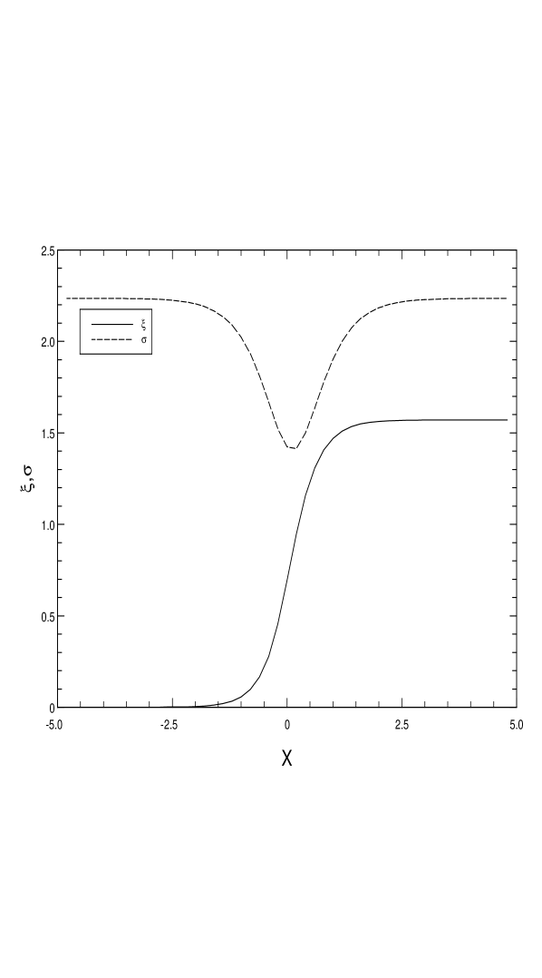
Figure 1:

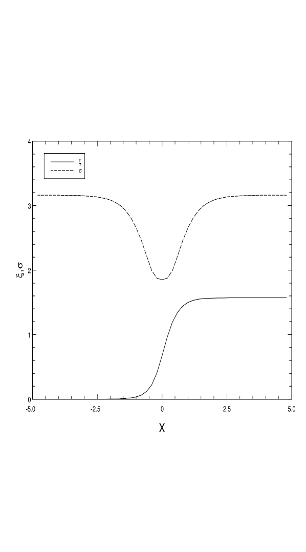
Figure 2:

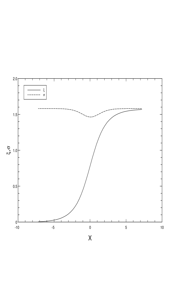
Figure 3:

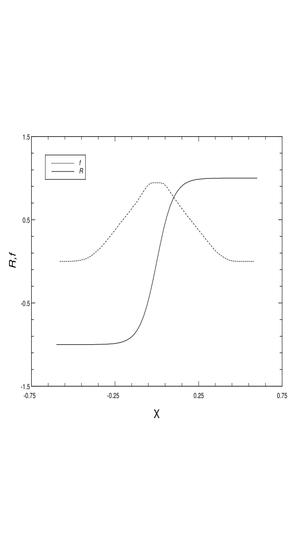
Figure 4:

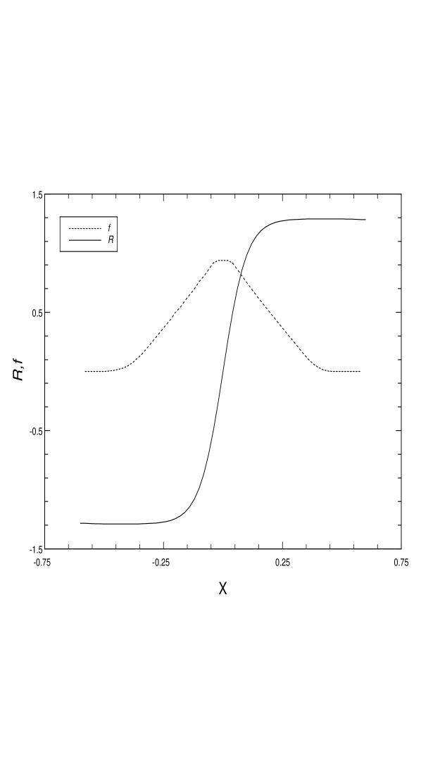
Figure 5:

Figure 6:

References

- [1] T. W. B. Kibble, J. Phys. A9, 1387 (1976).
- [2] See for example “ Classical lumps and their quantum descendants” in S. Coleman, Aspects of Symmetry (Cambridge University Press, 1985.)
-
[3]
T. W. B. Kibble, Phys. Rep. 67, 183 (1980);
M. Hindmarch and T. W. B. Kibble, Rep. Prog. Phys. 58, 477 (1995). - [4] S. Bhowmik Duari and U. A. Yajnik, Phys. Lett. B 326, 212 (1994).
- [5] R. Brandenberger, A-C. Davis, and M. Trodden, Phys. Lett. B 335, 123 (1994).
-
[6]
J. Garriga and T. Vachaspati, Nucl. Phys. B438,
161 (1995);
M. Barriola, Phys. Rev. D 51, 300 (1995). - [7] R. Brandenberger, A-C. Davis, T. Prokopec and M. Trodden, Phys. Rev. D 53, 4257 (1996).
- [8] For a recent review, see T. Vachaspati, hep-ph 9710292.
- [9] J. Preskill, Phys. Rev. Lett. 43, 1365 (1979).
- [10] A. Vilenkin and E. P. S. Shellard, Cosmic Strings And Other Topological Defects (Cambridge University Press, Cambridge, 1994.)
- [11] Ya. B. Zel’dovich, I. Yu. Kobzarev and L. B. Okun, JETP Lett. 40, 1 (1974).
- [12] G. Dvali, H. Liu and T. Vachaspati, Phys. Rev. Lett. 80, 2281 (1998).
- [13] S. Weinberg, Phys. Rev. D 9, 3357 (1974).
- [14] G. Senjanovic and R. N. Mohapatra, Phys. Rev. D 12, 1502 (1975).
- [15] R. N. Mohapatra and G. Senjanovic, Phys. Rev. Lett. 44, 912 (1980), Phys. Rev. D 23, 165 (1981).
- [16] G. Dvali and G. Senjanovic, Phys. Rev. Lett. 74, 5178 (1995).
- [17] G. Dvali, A. Melfo and G. Senjanovic, Phys. Rev. D 54, 7857 (1996).
- [18] G. Dvali, A. Melfo and G. Senjanovic, Phys. Rev. Lett. 74, 4559 (1995).
- [19] B. Bajic, A. Riotto and G. Senjanovic, Phys. Rev. Lett. 81, 1355 (1998).
- [20] A. D. Sakharov, JETP Lett. 5, 24 (1967).
- [21] R. Brandenberger, A.-C. Davis, T. Prokopec and M. Trodden, Phys. Rev. D 53, 4257 (1996).
- [22] R. Brandenberger, I. Halperin and Z. Zhitnitsky, hep-ph/9808471.
- [23] A. Stern and U. A. Yajnik, Nucl. Phys. B267, 158 (1986).
- [24] U. A. Yajnik, Phys. Lett. B 184, 229 (1987).
-
[25]
A-C. Davis and S. C. Davis, Phys. Rev. D 55, 1879
(1986);
S. C. Davis, A-C. Davis and W. B. Perkins, Phys. Lett. B 408, 81 (1998). -
[26]
A. I. Bochkarev and M. E. Shaposhnikov,
Mod. Phys. Lett. A2, 417 (1987);
A. I. Bochkarev, S. Yu. Khlebnikov and M. E. Shaposhnikov, Nucl. Phys. B329, 490 (1990). - [27] M. Carena, M. Quiros and C. Wagner, Phys. Lett. B 380, 81 (1996)
- [28] M. Carena, M. Quiros, A. Riotto, I. Vilja and C. E. M. Wagner, Nucl. Phys. B503, 387 (1997).
- [29] J. Cline, M. Joyce and K. Kainulainen, Phys. Lett. B 417, 79 (1998).
- [30] R. Jeannerot, Phys. Rev. Lett. 77, 3292 (1996).
-
[31]
J. C. Pati and A. Salam, Phys. Rev. D 10, 275 (1975);
R. N. Mohapatra and J. C. Pati, ibid 11, 566, 2558 (1975). - [32] R. N. Mohapatra, Unification And Supersymmetry (Springer-Verlag, New York, 1992).
- [33] N. G. Deshpande, J. F. Gunion, B. Kayser and F. Olness, Phys. Rev. D 44, 3320 (1991).
- [34] We note that this reasoning does not apply to the standard model Higgs sector because it is a doublet and does not belong to the stability group of its vev.
-
[35]
R. Jackiw and P. Rossi, Nucl. Phys. B190, 681 (1981);
E. Weinberg Phys. Rev. D 24, 2669 (1981). - [36] J. F. Gunion, H. E. Haber, G. Kane and S. Dawson, The Higgs Hunter’s Guide (Addison-Wesely Publishing Company 1990).
-
[37]
T. Kibble, G. Lazarides and Q. Shafi,
Phys. Lett. B 113, 237 (1982) ;
T. Kibble, G. Lazarides and Q. Shafi, Phys. Rev. D 26, 435 (1982). - [38] R. Mohapatra and X. Zhang, Phys. Rev. D 46, 5331 (1992).
- [39] J.-M. , L. Houart, J. M. Moreno, J. Orloff and M. Tytgat, Phys. Lett. B 314, 289 (1993).
- [40] G. Barenboim and J. , Z. Phys. C 73, 321 (1997).
- [41] L. Reina and M. Tytgat, Phys. Rev. D 50, 751 (1994).
- [42] S. Ben-Menahem and A. S. Cooper, Nucl. Phys. B388, 409 (1992).
- [43] H. Lew and A. Riotto, Phys. Lett. B 309, 258 (1993).
- [44] R. Brandenberger and A.-C. Davis, Phys. Lett. B 308, 79 (1993).