Non SUSY Unification in Left-Right Models.

Abstract

We explore in a model independent way the possibility of achieving the non supersymmetric gauge coupling unification within left-right symmetric models, with the minimal particle content at the left-right mass scale which could be as low as 1 TeV in a variety of models, and with a unification scale M in the range $10^{5}$ GeV $<M<10^{17.7}$ GeV.

Pacs: 11.10.Hi;12.10.-g;12.10.Kt

1 Introduction

It has been known for more than a decade[1] that if we let the three gauge couplings $c_{i}\alpha_{i}^{-1}$ run through the “desert” from low to high energies, they do not merge together into a single point, where $\{c_{1},c_{2},c_{3}\}=\{\frac{3}{5},1,1\}$ are the normalization constants of the Standard Model (SM) factors U(1)_Y, SU(2)_L and SU(3)_c, respectively, embedded into SU(5)[2]. This odd result claims for new physics at intermediate energy scales as for example:

1. The inclusion of the minimal supersymmetric (SUSY) partners of the SM fields at an energy scale $M_{susy}\sim 1$ TeV, related to an unification scale $M\sim 10^{16}$ GeV[3].

2. The inclusion of a minimal Left Right Symmetric Model (LRSM) at a mass scale $M_{R}\sim 10^{11}$ GeV, related to an unification scale $M\sim 10^{15}$ GeV[4] in an SO(10) Grand Unified Theory (GUT) [5].

3. The inclusion of the SUSY partners of the minimal LRSM at an energy scale $M_{susy}\sim M_{R}\sim 1$ TeV, related to a unification scale $M\sim 10^{16}$ GeV[6]. Etc..

The alternative approach, namely, to normalize the gauge couplings $c_{i}\alpha_{i}^{-1}$ to non-orthodox $c_{i},\;(i=1,2,3)$ values was presented by these authors, in Ref. [7] for non-SUSY models, and in Ref. [8] for the SUSY ones, for possible GUT models which can descend in one single step to $SU(3)_{c}\otimes SU(2)_{L}\otimes U(1)_{Y}\equiv G_{SM}$.

In this paper we present a systematic analysis of all the possible GUT models which descend in two steps to $G_{SM}$, with the LRSM as the intermediate step, paying special attention to those models with low $M_{R}$ scale. The paper is organized in the following way: In section II we present the renormalization group equation formalism for the LRSM; in section III we carry our model independent analysis, and in section IV we present our results and conclusions. A technical appendix at the end gives the $c_{i},\;i=1,2,3$ values for most of the GUT models in the literature.

2 The Renormalization Group Equations

In a field theory, the couplings are defined as effective values, which are energy scale dependent according to the renormalization group equations. In the modified minimal substration scheme  [9], which we adopt in what follows, the one-loop renormalization group equations are

$$\mu{d\alpha_{i}\over d\mu}\simeq-b_{i}\alpha_{i}^{2},$$ (1)

where $\mu$ is the energy at which the coupling constants $\alpha_{i}=g_{i}^{2}/4\pi,\,(i=1,2,3)$ are evaluated, with $g_{1}$, $g_{2}$, and $g_{3}$ the gauge couplings of the SM factors $U(1)_{Y}$, $SU(2)_{L}$ and $SU(3)_{c}$ respectively. The constants $b_{i}$ are completely determinated by the particle content in the model by

$$4\pi b_{i}={11\over 3}C_{i}(vectors)-{2\over 3}C_{i}(fermions)-{1\over 3}C_{i}(scalars),$$

being $C_{i}(\cdots)$ the index of the representation to which the $(\cdots)$ particles are assigned, and where we are considering Weyl fermion and complex scalar fields [10]. The boundary conditions for these equations are determined by the relationships

$$\alpha^{-1}_{em}=\alpha_{1}^{-1}+\alpha_{2}^{-1},\quad\mbox{and}\quad\tan^{2}\theta_{W}={\alpha_{1}\over\alpha_{2}},$$ (2)

which at the electroweak scale imply

$$\alpha_{1}^{-1}(m_{Z})=\frac{1-{\rm sin}^{2}\theta_{W}(m_{Z})}{\alpha_{em}(m_{Z})},\quad\mbox{and}\quad\alpha_{2}^{-1}(m_{Z})=\frac{{\rm sin}^{2}\theta_{W}(m_{Z})}{\alpha_{em}(m_{Z})}.$$ (3)

Combining those expressions with the experimental values

$$\alpha^{-1}_{em}(m_{Z}) = 127.90\pm 0.09~{}\cite[cite]{[\@@bibref{}{pdg,ewk}{}{}]},$$

$$\sin^{2}\theta_{W}(m_{Z}) = 0.2312\pm 0.00017~{}\cite[cite]{[\@@bibref{}{pdg,ewk}{}{}]}\quad\mbox{and}$$ (4)

$$\alpha_{3}(m_{Z}) = \alpha_{s}=0.1191\pm 0.0018~{}\cite[cite]{[\@@bibref{}{pdg}{}{}]},$$

we get:

$$\alpha^{-1}_{1}(m_{Z}) = 98.330\pm 0.091,$$

$$\alpha^{-1}_{2}(m_{Z}) = 29.571\pm 0.043,\quad\mbox{and}$$ (5)

$$\alpha^{-1}_{3}(m_{Z}) = 8.396\pm 0.127.$$

The unification of the three SM gauge couplings is properly achieved if they meet together into a common value $\alpha=g^{2}/4\pi$ at a certain energy scale $M$, where $g$ is the gauge coupling constant of the unifying group $G$. However, since $G\supset G_{SM}$, the normalization of the generators corresponding to the subgroups $U(1)_{Y}$, $SU(2)_{L}$ and $SU(3)_{c}$ is in general different for each particular group $G$, and therefore the SM coupling constants $\alpha_{i}$ differ at the unification scale from $\alpha$ by numerical factors $c_{i}\,(\alpha_{i}=c_{i}\alpha)$. In $SU(5)$ these factors are[2] $\{c_{1},c_{2},c_{3}\}=\{{3\over 5},1,1\}$ (we call them the canonical values), which are the same for $SO(10)$ [5], $E_{6}$ [13], $[SU(3)]^{3}\times Z_{3}$[14], $SO(18)$[15], $E_{8}$[16], $SU(15)$[17], $SU(16)$[18], and $SU(8)\otimes SU(8)$[19], but they are different for other groups such as $SU(5)\otimes SU(5)$ [20], $[SU(6)]^{3}\times Z_{3}$[21], the Pati-Salam models[22], etc. (see Table I in the appendix).

The constants $c_{i}$ can also be seen as a consequence of the affine levels (or Kac-Moody levels) at which the gauge factor $G_{i}$ is realized in the effective four dimensional string[23], even if there is not an unification gauge group at all; but if it does, they are related to the fermion content of the irreducible representations of $G$. As a matter of fact, if $\alpha_{i}$ is the coupling constant of $G_{i}$, a simple group embedded into $G$, then

$$c_{i}\equiv{\alpha_{i}\over\alpha}={Tr\ T^{2}\over Tr\ T^{2}_{i}},$$ (6)

where $T$ is a generator of the subgroup $G_{i}$ properly normalized over a representation $R$ of $G$, and $T_{i}$ is the same generator but normalized over the representation of $G_{i}$ embedded into $R$ (the traces run over complete representations). In this way for example, if just one standard doublet of $SU(2)_{L}$ is contained in the fundamental representation of $G$ (plus any number of $SU(2)_{L}$ singlets), then $c_{2}=1$ (as in $SU(5)$); but this is not the general case. In this way we proof that for $i=2,3$, $c_{i}^{-1}=1,2,3,...n$ an integer number. The constants $c_{i}$ are thus pure rational numbers satisfying $c_{1}>0$ and $0<c_{2(3)}\leq 1$. They are fixed once we fix the unifying gauge structure. According to the table I in the appendix and in order to simplify matters, we are going to use for $c_{2}$ only the values $1$ and ${1\over 3}$, and for $c_{3}$ the values 1 and ${1\over 2}$.

From Eqs. (2) and (6) it follows that at the unification scale the value of $\sin^{2}\theta_{W}$ is given by

$$\sin^{2}\theta_{W}\equiv{\alpha_{em}\over\alpha_{2}}={c_{1}\over c_{1}+c_{2}}.$$ (7)

Obviously, Eq. (7) is equivalent to that given in terms of the traces of the generators of $SU(2)_{L}$ and the electric charge for simple groups (see Ref. [2]). In order to connect this value at the scale $M$ with the corresponding value at the scale $m_{Z}$ the renormalization group equations (1) must be solved.

Our approach is now the following: we assume there are only three relevant mass scales $m_{Z},\,M_{R}$, and $M$ such that $m_{Z}<M_{R}<M$, where $m_{Z}\sim 10^{2}$GeV is the electroweak mass scale, $M_{R}$ is the mass scale where the LRSM (with and without discrete left-right (LR) symmetry) manifests itself, and $M$ is the GUT scale. Then, the equations (1) must be solved, first for the energy range $m_{Z}<\mu<M_{R}$, and then for the range $M_{R}<\mu<M$, properly using at each stage the decoupling theorem [24].

Now for the energy interval $m_{Z}<\mu<M_{R}$, the one loop solutions to the equations (1) are:

$$\alpha_{i}^{-1}(m_{Z})=\alpha_{i}^{-1}(M_{R})-b_{i}(H)\,\ln\left({M_{R}\over m_{Z}}\right),$$ (8)

where the beta functions $b_{i}\,(i=1,2,3)$ are [10]

$$2\pi\left(\begin{array}[]{c}b_{1}\\[5.16666pt] b_{2}\\[5.16666pt] b_{3}\end{array}\right)=\left(\begin{array}[]{c}0\\[5.16666pt] 22\over 3\\[5.16666pt] 11\end{array}\right)-\left(\begin{array}[]{c}20\over 9\\[5.16666pt] 4\over 3\\[5.16666pt] 4\over 3\end{array}\right)F-\left(\begin{array}[]{c}1\over 6\\[5.16666pt] 1\over 6\\[5.16666pt] 0\end{array}\right)H,$$ (9)

with $F=3$ the number of families and $H$ the number of low energy Higgs field doublets. Notice by the way that we are not including in the former equation the normalization factor $3\over 5$ into $b_{1}$ coming from $SU(5)$, and wrongly included in some general discussions. $H=1$ in the SM; nevertheless, a general model can have more than one low energy Higgs field, and in principle $H$ may be taken as a free parameter ($H=2$ in the minimal supersymmetric model).

For the interval $M_{R}<\mu<M$, the evolution of the gauge couplings is dictated by the beta functions of the LRSM whose gauge group is [25] $G_{LR}\equiv SU(3)_{c}\otimes SU(2)_{L}\otimes SU(2)_{R}\otimes U(1)_{B-L}$, with the matter fields transforming as $\Psi_{L}=(3,2,1,1/6)\oplus(\bar{3},1,2,-1/6)\oplus(1,2,1,-1/2)\oplus(1,1,2,1/2)$ for each generation, where the numbers between brackets label ($SU(3)_{c},SU(2)_{L}$, $SU(2)_{R}$, $U(1)_{B-L}$) representations.

The LRSM is broken down spontaneously by the Higgs sector, which in general contains $N_{B}$ bidoublet Higgs fields $\varphi(1,2,2,0)$, $N_{TL}$ triplets in the representation $\Delta_{L}(1,3,1,1)$, $N_{TR}$ triplets in the representation $\Delta_{R}(1,1,3,-1)$, $N_{DL}$ doublets in the representation $\phi_{L}(1,2,1,-1/2)$, and $N_{DR}$ doublets in the representation $\phi_{R}(1,1,2,1/2)$. In the so called minimal LRSM[25], $N_{TR}=N_{B}=1$ and $N_{DL}=N_{DR}=N_{TL}=0$, but in general $N_{TL},\,N_{TR},\,N_{DL},\,N_{DR}$ and $N_{B}$ should be taken as free parameters to be fixed by the specific model.

In a general context, the vacuum expectation values that may be used to break the symmetry are $\langle\Delta_{R}^{0}\rangle\sim\langle\phi^{0}_{R}\rangle\sim M_{R}\;(\Delta_{R}^{0}$ represent the electromagnetic neutral direction in $\Delta_{R}$, etc.), $\langle\varphi^{0}\rangle\sim\langle\phi^{0}_{L}\rangle\sim m_{Z}$, and $\langle\Delta^{0}_{L}\rangle=0$. It then follows that $H=2N_{B}+N_{DL}$.

The discrete LR symmetry implies invariance under the exchange $L\leftrightarrow R$ in the model (this is the so called D parity) with the consequence that $g_{2L}=g_{2R}$ for the energy interval $M_{R}<\mu<M$. This symmetry is respected by the gauge and the fermion content of any LRSM, but it is broken by the scalar sector as it is shown anon.

Indeed, the Higgs field scalars can drastically alter the solution to the renormalization group equations, and in order to make any definite statement about the mass scales in a particular model, we must know which components of the Higgs representations have masses of order $m_{Z},\;M_{R}$ and $M$. However, to know the masses of the scalars is equivalent to the hopeless task of knowing the values of all the coupling constants appearing in the scalar potential (with radiative corrections included). So, in order to guess what the real effect of the scalars is, the so called extended survival hypothesis was introduced in Ref. [26]. Basically the hypothesis consists in assuming that only the components of the Higgs representations which are required for the breaking of a particular symmetry are the only ones which are not superheavy. In other words: “scalar Higgs fields acquire the maximum mass compatible with the pattern of symmetry breaking” (for a more detailed explanation and application to SO(10), see Ref. [26]).

The one loop solutions to Eqs. (1) for the energy interval $M_{R}<\mu<M$ are:

$$\alpha_{i}^{-1}(M_{R})={1\over c_{i}}\alpha^{-1}-b^{\prime}_{i}(N_{B},N_{TL},N_{TR},N_{DL},N_{DR})\,\ln\left({M\over M_{R}}\right),$$ (10)

where $i=BL,2L,2R,3$. The beta functions $b^{\prime}_{i}$ are now: $b^{\prime}_{3}=b_{3}=7/2\pi$ (with the assumption that no low energy colored scalars exist (as demanded by the extended survival hypothesis); if they do, they may cause a too fast proton decay, and spoil the asymptotic freedom for $SU(3)_{c}$); and $b^{\prime}_{2R},\,b^{\prime}_{2L}$ and $b^{\prime}_{BL}$ given by:

$$2\pi\left(\begin{array}[]{c}b^{\prime}_{BL}\\[5.16666pt] b^{\prime}_{2L}\\[5.16666pt] b^{\prime}_{2R}\end{array}\right) = \left(\begin{array}[]{c}0\\[5.16666pt] 22\over 3\\[5.16666pt] 22\over 3\end{array}\right)-\left(\begin{array}[]{c}8\over 9\\[5.16666pt] 4\over 3\\[5.16666pt] 4\over 3\end{array}\right)F-\left(\begin{array}[]{c}0\\[5.16666pt] N_{B}\over 3\\[5.16666pt] N_{B}\over 3\end{array}\right)-\left(\begin{array}[]{c}N_{TL}+N_{TR}\\[5.16666pt] \frac{2N_{TL}}{3}\\[5.16666pt] \frac{2N_{TR}}{3}\end{array}\right)-\left(\begin{array}[]{c}\frac{N_{DL}+N_{DR}}{6}\\[5.16666pt] \frac{N_{DL}}{6}\\[5.16666pt] \frac{N_{DR}}{6}\end{array}\right).$$ (29)

From Eqs. (10) and (29) we get $g_{2L}=g_{2R}$ if $N_{TL}=N_{TR}$ and $N_{DL}=N_{DR}$. But if $N_{TR}\neq N_{TL}=0$ as demanded by the extended survival hypothesis, then one could only have exact left-right symmetry at the GUT scale.

The hypercharge $Y$ of the SM is given by

$$Y=T_{3R}+Y_{B-L},$$ (30)

which implys the relation $\alpha_{1}^{-1}(M_{R})=\alpha_{2R}^{-1}(M_{R})+\alpha_{BL}^{-1}(M_{R})$. Then the beta function for $U(1)_{Y}$ for the energy interval $M_{R}<\mu<M$ may be written as $b_{1}^{\prime}=b^{\prime}_{2R}+b^{\prime}_{BL}$ with $c_{1}^{-1}=c_{2R}^{-1}+c_{BL}^{-1}$, and $c_{2R}=c_{2L}=c_{2}$, ($c^{-1}_{BL}={2\over 3}$ for the minimal fermion field content of the LRSM). These relations together with Eqs. (8) and (10) allow us to write:

$$\alpha_{1}^{-1}(m_{Z}) = {1\over c_{1}}\alpha^{-1}+\left(\frac{40+H}{12\pi}\right)\,\ln\left({M\over m_{Z}}\right)-\frac{1}{6\pi}(22-3N_{TL}-5N_{TR}-N_{DR})\,\ln\left(M\over M_{R}\right)$$

$$\alpha_{2}^{-1}(m_{Z}) = {1\over c_{2}}\alpha^{-1}-\frac{1}{12\pi}\left[(20-H)\,\ln\left({M\over m_{Z}}\right)-4N_{TL}\,\ln\left({M\over M_{R}}\right)\right]$$ (31)

$$\alpha_{3}^{-1}(m_{Z}) = {1\over c_{3}}\alpha^{-1}-\frac{7}{2\pi}\,\ln\left({M\over m_{Z}}\right),$$

which is a system of 3 equations with 3 unknowns: $\alpha,\;M_{R}$ and $M$ ($m_{Z}=91.187\pm 0.007$ GeV[11] and $\alpha_{i}^{-1}(m_{Z})$ as in Eqs. (5) are taken as imputs). $c_{i}(i=1,2,3)$, $N_{B},N_{TL},N_{TR},N_{DL}$, and $N_{DR}$ $(H=2N_{B}+N_{DL})$ are model dependent parameters. Evidently, there is always solution to the system of equations in (31), but the consistency of the unification scheme demands that $m_{Z}<M_{R}<M\leq 10^{19}$ GeV$\sim M_{P}$ (the Planck Mass). When we solve Eqs. (31) for the minimal LRSM $(N_{TR}=N_{B}=1,\,N_{TL}=N_{DL}=N_{DR}=0)$ for the canonical values $(\{c_{1},c_{2},c_{3}\}=\{{3\over 5},1,1\})$ we get $M=2.5\;10^{16}$ GeV, $M_{R}=2.7\;10^{9}$ GeV and $\alpha^{-1}=45.45$.

Notice that if $N_{TL}=0$ (as demanded by the extended survival hypothesis), the last two equations in (31) are independent of $M_{R}$, and they are enough to fix the GUT scale $M$ (and $\alpha$ of course). If we solve them for $c_{2}=1,\,c_{3}={1\over 2}$ (one family models with chiral color[27], as for example $SU(5)\otimes SU(5)$[20], $SO(10)\otimes SO(10)$ [28]), we get for $H<22$ the unphysical solution $M>>M_{P}$. A further analysis shows that for $22<H<30$ we get $M_{P}>M>10^{16}$ GeV which in turn implies $M_{R}<m_{Z}$ which is also unphysical. To get $M_{R}>1$ TeV requires for those models $H>40$ which gives $M<10^{12}$ GeV in serious conflict with proton decay which is always present in those models. So the two step breaking pattern $SU(5)\otimes SU(5)\longrightarrow G_{LR}\longrightarrow G_{SM}$ is not allowed (the one step $SU(5)\otimes SU(5)\longrightarrow G_{SM}$ is also forbidden[7, 8]). This conclusion is valid even for the case $g_{2L}\neq g_{2R}$ at the GUT scale, a variant of the model introduced in the second paper of Ref. [20]. Similar conclusions follow for $SO(10)\otimes SO(10)$ [28]. To use $N_{TL}\neq 0$ makes things even worse.

When we solve Eqs.(31) for $c_{2}={1\over 3},\,c_{3}=1$ (models with three families and vector-like color as for example $[SU(6)]^{3}\times Z_{3}$ [21]) we get $M\simeq 5m_{Z}$, an unacceptable solution. So the two step breaking pattern $[SU(6)]^{3}\times Z_{3}\longrightarrow G_{LR}\longrightarrow G_{SM}$ is not allowed either (the one step breaking pattern $[SU(6)]^{3}\times Z_{3}\longrightarrow G_{SM}$ is also forbidden for this group[7, 8]).

So our analysis makes sense only for two cases: $\{c_{2},c_{3}\}=\{1,1\}$ (one family models with vector like-color), and $\{c_{2},c_{3}\}=\{{1\over 3},{1\over 2}\}$ (models with 3 families and chiral color). In what follows we are going to refer only to these situations.

Before moving to a general analysis, let us see for example what happens for $SO(10)\longrightarrow G_{LR}\longrightarrow G_{SM}$. As mentioned above, $\{c_{1},c_{2},c_{3}\}=\{{3\over 5},1,1\}$, and there are not exotic fermions in the spinorial 16 representation used for the matter fields, but the scalar content is not quite uniquely defined, and there are as many versions of the model as you wish. A couple of examples are:
1- In Ref.[4] the following symmetry breaking pattern is implemented:

$$SO(10)\stackrel{{\scriptstyle\phi_{(210)}}}{{\longrightarrow}}G_{LR}\stackrel{{\scriptstyle\phi_{(126)}}}{{\longrightarrow}}G_{SM}\stackrel{{\scriptstyle 2\phi_{(10)}}}{{\longrightarrow}}SU(3)_{c}\otimes U(1)_{EM}.$$

$\phi_{210}$ gets mass at the GUT scale and it does not contribute to the renormalization group equations. For $\phi_{126},\;\Delta_{R}=\Delta_{L}=1$, but only $\langle\Delta_{R}\rangle\neq 0$. For the final breaking only one $\phi_{(10)}$ is needed, but at least two must be used in order to achieve proper isospin breaking. Then $N_{TR}=1,\;N_{B}=2,\;N_{TL}=N_{DL}=N_{DR}=0$. We get $M=2.0\;10^{15}$ GeV, $M_{R}=1.6\;10^{11}$ GeV and $\alpha^{-1}=42.6$.
2- A more recent version of (SUSY) S0(10) implements the breaking with the following scalar content[29]:

$$SO(10)\stackrel{{\scriptstyle\phi_{(45)}}}{{\longrightarrow}}G_{LR}\stackrel{{\scriptstyle\phi_{(16+cc)}}}{{\longrightarrow}}G_{SM}\stackrel{{\scriptstyle 2\phi_{(10+16+cc)}}}{{\longrightarrow}}SU(3)_{c}\otimes U(1)_{EM}.$$

With the extended survival hypothesis in mind we have $N_{TL}=N_{TR}=0,\;N_{B}=N_{DL}=N_{DR}=2$. We get $M=2.2\;10^{14}$ GeV, $M_{R}=9\;10^{12}$ GeV, and $\alpha^{-1}=40.16$. In both examples the D parity is broken below the GUT scale.

Since the scalar sector is the most obscure part of any gauge theory, it is clear that, $N_{i}\;(i=B,TL,TR,DL$ and $DR)$ can be taken as free parameters, resulting in all sort of models for all sort of tastes. Since the Higgs field scalars can drastically change the GUT scales, we can not state with confidence neat values for $M$ and $M_{R}$. We elaborate on this in the next section.

Before proceeding to our model independent analysis let us mention that we are going to consider the possibility of adding arbitrary large numbers of scalars Higgs fields in order to get unification. In many cases this may result in the coupling constants becoming so large as to make the theory non-perturbative before unification is achieved. Even though the extended survival hypothesis[26] greatly diminishes the effect of the Higgs scalar fields, we will pay special attention to our parameter space region in the analysis, in order not to run into non-perturbative regimes of the coupling constants. As a mater of fact, the assumption that no low energy colored scalars exist is all what is needed for the cases considered ahead.

3 Model Independent Analysis

In this section we are going to study two different situations. First we are going to reduce the freedom we have in our parameter space by imposing the extended survival hypothesis. Second, we reduce the freedom by restoring the D parity to the LRSM.

3.1 Solutions to the equations with extended survival hypothesis

If we impose the extended survival hypothesis as a constraint in the solutions to the renormalization group equations for the LRSM, we must set $N_{TL}=0$. Then Eqs. (31) get reduced to a system of 3 equations with 3 unknowns, and the following set of parameters: $c_{i}$ $(i=1;2;3)$; $H$, and $N^{\prime}_{T}=5N_{TR}+N_{DR}$. The solution of Eqs. (31) for $M$, $M_{R}$ and $\alpha$ as functions of these parameters is:

$$\alpha^{-1} = \frac{42t_{32}-(20-H)t_{23}}{D}$$ (32)

$$\ln\left({M\over m_{z}}\right) = \frac{12\pi}{D}\left[c_{2}\alpha^{-1}_{2}(m_{Z})-c_{3}\alpha^{-1}_{3}(m_{Z})\right]$$ (33)

and

$$\ln\left({M\over M_{R}}\right)=\frac{6\pi N}{c_{1}(22-N^{\prime}_{T})D}$$ (34)

where $N=[(20-H)(t_{21}-t_{23})+(40+H)(t_{12}-t_{13})+42(t_{32}-t_{31})]$, $D=42c_{3}-(20-H)c_{2}$ and $t_{ij}=t_{ij}(m_{Z})=c_{i}c_{j}\alpha^{-1}_{j}(m_{Z})$. From Eq. (34) it can be seen that either $H<7$ and $N^{\prime}_{T}<22$ ($N_{TR}<5$), or $H>7$ and $N^{\prime}_{T}>22$, in order to have $M_{R}\leq M$.

From Eqs. (33) and (34) we plot in Figure 1 the allowed region for $H$ and $N^{\prime}_{T}$ that give unification, for the canonical values of $c_{i}$; and in Figure 2 we plot $c_{1}$ Versus $N^{\prime}_{T}$ for $H=2$ and $\{c_{2};c_{3}\}=\{{1\over 3};{1\over 2}\}$.

To analyze the implications of each one of the figures we must have in mind the following constraints:

1. $M\leq M_{P}\sim 10^{19}$ GeV, the Planck scale (actually $M\leq M_{max}\sim 10^{17.7}$ GeV, obtained when there is not contribution from the scalar sector).

2. $M>10^{5}$ GeV in order to suppress unwanted flavor changing neutral currents [11, 30].

3. $M>10^{16}$ if the proton is allowed to decay in the particular GUT model.

4. $8\,m_{Z}\leq M_{R}\leq M$. The lower limit is taken from the particle data book[11], the upper limit is imposed by consistency of the renormalization group equations.

3.1.1 Analysis of Figure 1.

The allowed region lies inside the lines $M_{R}=8\,m_{Z}$ and $M_{R}=M$, but if the proton does decay in the model under consideration then the allowed region lies in the lower left corner between the lines $M=10^{16}$ GeV, $M_{R}=8\,m_{Z}$, $H=0$ and $N^{\prime}_{T}=0$.

For GUT models with unstable proton (which are most of the models for the groups in the canonical entry in Table 1 in the appendix), $M_{R}\sim 1$ TeV is obtained for $H=2$ and $N^{\prime}_{T}=13$ ($N_{TR}=2$ and $N_{DR}=3$), which in turn implies $M\sim 2.59\;10^{16}$ GeV.

For models in the canonical entry with a stable proton (as for example $[SU(3)]^{3}\times Z_{3}$[14] and $SU(8)\otimes SU(8)$[19]) the allowed region is wider and divided in two regions. One for $H<7$; $N^{\prime}_{T}<22$ and the other for $H>7$ and $N_{T}>22$. There are plenty of examples of models with $M_{R}\sim 1$ TeV for those situations.

3.1.2 Analysis of Figure 2.

The entire plane in figure 2 is related to the GUT scale $M\sim 10^{8}$ GeV (fixed just by the values of $H,\;c_{2}$ and $c_{3}$). The allowed region lies between the lines $M_{R}=M$ and $M_{R}=8\,m_{Z}$. From the figure we see that a value of $c_{1}={3\over 19}$ crosses the $M_{R}=8\,m_{Z}$ line at $N^{\prime}_{T}=31\;(N_{TR}=6,\;N_{DR}=1)$, which means that the model $[SU(6)]^{4}\times Z_{4}$[31] can have the following chain of spontaneous descent

$$[SU(6)]^{4}\times Z_{4}\stackrel{{\scriptstyle M}}{{\longrightarrow}}G_{LR}\stackrel{{\scriptstyle M_{R}}}{{\longrightarrow}}G_{SM}\stackrel{{\scriptstyle m_{Z}}}{{\longrightarrow}}SU(3)_{c}\otimes U(1)_{EM},$$

with $M\sim 10^{8}$ GeV and $M_{R}\sim 9\,m_{Z}$, as long as an irreducible representation of the GUT group with 6 right handed triplets is used to break $G_{LR}$ down to the SM gauge group and then a representation of the GUT group with only two $SU(2)_{L}$ Higgs field doublets is used in the last breaking step.

A further look into the equations for this group shows that for $N^{\prime}_{T}=0$ and $H=2,3$ we get $M_{R}=M\sim 10^{8}$ GeV, meaning that a single step spontaneous descent is possible for this model with a very economical set of Higgs field scalars. But this result has been already published in Ref.[7]. Here we just confirm the published result.

3.2 Solutions to the equations with D parity

In order to restore the D parity in the renormalization group equations for the energy interval $M_{R}<\mu<M$ we must have $N_{TL}=N_{TR}\equiv N_{T}$ and $N_{DL}=N_{DR}=N_{D}$. Again we solve Eqs. (31) as a function of $c_{i}$, $H$, $N_{T}$ and $N_{D}$. Using the equations we get, we plot in Figure 3 the allowed region for $H$ and $N_{T}$ that gives unification for the canonical values of $c_{i}$, and in Figure 4 we plot $c_{1}$ Versus $N_{T}$ for $H=2$, $N_{D}=0$ and $\{c_{2};c_{3}\}=\{1;1\}$.

3.2.1 Analysis of Figure 3

For models with unstable proton the allowed tiny region lies in the lower left corner, between the lines $N_{T}=0,\;H=0$ and $M=10^{16}$ GeV. From the figure we get $M_{R}>10^{9}$ GeV, $N_{T}\leq 1$ and $H\leq 2$.

For models with an stable proton the allowed region is larger, with boundaries given by the lines $M_{R}=M$ and $M=10^{5}$ GeV which excludes the possibility $M_{R}\sim$ a few TeV, unless $N_{T}>50$ which is very unlikely in realistic models.

3.2.2 Analysis of Figure 4

The allowed region of parameters lies inside the lines $N_{T}=0,\;M=M_{R}$ and $M=10^{16}$ GeV for models with unstable proton, and inside the lines $N_{T}=0,\;M=M_{R}$ and $M_{R}=8\,m_{Z}$ for models with an stable proton. As can be seen, the canonical value $c_{1}={3\over 5}$ lies inside both regions, but far from $M_{R}\sim 1$ TeV.

In general, large values for $N_{T}$ are required $(H<8)$ in LRSM with D parity, in order not to have unduly large values for $M_{R}$.

4 Conclusions

To conclude let us emphasize that it is possible to unify the SM group using the LRSM as an intermediate stage for a variety of models, with 1 TeV $\leq M_{R}\leq 10^{15}$ GeV. From our study, three family models with vector like color are excluded (as $[SU(6)]^{3}\times Z_{3}$), and one family models with chiral color are also excluded (as $SU(5)\otimes SU(5)$ [20], and $SO(10)\otimes SO(10)$ [28]).

We point out that in our analysis we have neglected threshold effects which depend on the particular structure of each model, and also we do not include second order corrections to the renormalization group equations which are typically of the order of the threshold effects. In others aspects it is completely general. Within this limitations we may conclude that it is indeed possible to achieve the unification of the coupling constants of the SM in a general class of non supersymmetric models which have the minimal LRSM as an intermediate step, with an $M_{R}$ scale as low as 1 TeV. We are aware that this class of models may suffer of hierarchy problems.

From our analysis we may extract the following morals:
1- Higgs scalars play a crucial role in the solution to the renormalization group equations.
2- It is simple to construct realistic non SUSY - GUT models with an intermediate Left-Right symmetry at a mass scale $M_{R}\sim 1$ TeV (just read them from the figures).
3- LRSM with D parity are quite different to those without D parity.
4- For low $M_{R}$, models with D parity are less realistic that models without D parity, in the sense that they make use of a very large amount of Higgs scalars.
5- It is impossible to sustain the D parity when the extended survival hypothesis is imposed.

Appendix.

In this appendix we give the $c_{i}$ $i=1;2;3$ values for most of the GUT groups in the literature. They are presented in table I. The “Canonical” entry refers to the following groups: $SU(5)$ [2] $SO(10)$ [5], $E_{6}$ [13], $[SU(3)]^{3}\times Z_{3}$ [14], $SU(15)$ [17], $SU(16)$ [18], $SU(8)\times SU(8)$ [19], $E_{8}$ [16], and $SO(18)$ [15]. Also, in the Canonical entry we have normalized the $c_{i}$ values to the $SU(5)$ numbers; for example, the actual values for $SU(16)$ are: $\{c^{-1}_{1};c^{-1}_{2};c^{-1}_{3}\}=\{{20/3};4;4\}=4\{5/3;1;1\}$. This normalization makes sense because physical quantities such as sin${}^{2}\theta_{W}$, $M_{R}$ and $M$ depend only on ratios of two $c_{i}$ values (see Eqs. (7), (33), and (34)).

Most of the groups in the first entry have the canonical values for $c_{i}$ due to the fact that they contain $SU(5)$ via regular embeddings (see the table 58 in Ref.[32]), which do not change the rank of the corresponding group. For others as for example $SU(16)$ it is just an accident.

$c^{-1}_{3}$ can take only the values $1,2,3,4$ for one family groups, or higher integer values for family groups. $c^{-1}_{3}=1$ when it is $SU(3)c$ which is embedded in the GUT group $G$; $c^{-1}_{3}=2$ when it is the chiral color [27] $SU(3)_{cL}\times SU(3)_{cR}$ which is embedded in $G$, etc. For example $c^{-1}_{3}=4$ in $SU(16)$ due to the fact that the color group in the GUT group is $SU(3)_{cuR}\times SU(3)_{cdR}\times SU(3)_{cuL}\times SU(3)_{cdL}$.

For family groups $c^{-1}_{2}$ take the values $1,2,\dots F$ for $1,2,\dots F$ families. Indeed, the $c_{i}$ values for the $F$ family Pati-Salam models [33] $[SU(2F)]^{4}\times Z_{4}$ are $\{c^{-1}_{1};c^{-1}_{2};c^{-1}_{3}\}=\{(9F-8)/3;F;2\}$.

In general, $c^{-1}_{2(3)}=1,2,\dots f$, where $f$ is the number of fundamental representations of $SU(2)_{L}$ $(SU(3)_{c})$ contained in the fundamental representation of the GUT group. For example, $c_{2}^{-1}=4$ in $SU(16)$ because the 16 representation of $SU(16)$ contains four $SU(2)_{L}$ doublets; three for $(u,d)_{L}$ and one for $(\nu_{e},e)_{L}$.

The group $[SU(4)]^{3}\times Z_{3}$ in Table I is not the vector-like color version of the two family Pati-Salam group, but it is the one family theory introduced in Ref. [28]. Also, the group $[SU(6)]^{4}\times Z_{4}$ in the Table is not the 3 family Pati-Salam model, but a version of such model (with 3 families) without mirror fermions, introduced in Ref. [31].

All models in Table I are realistic, except $E_{7}$[34] which is a two family model with the right handed quarks in $SU(2)_{L}$ doublets.

The values $c_{i}$ (and Table I) are interesting by themselves because they are related to the Kac-Moody levels ($\kappa_{i}$) of String GUTs [23]. Indeed: $c^{-1}_{i}=\kappa_{i},\;i=1,2,3$. Curiously enough, the values for $c_{1}$ are integer multiple of 1/3 for all the known groups, we do not know why.

Group	$c^{-1}_{1}$	$c^{-1}_{2}$	$c^{-1}_{3}$
Canonical	5/3	1	1
$SU(5)\otimes SU(5)$	13/3	1	2
$SO(10)\otimes SO(10)$	13/3	1	2
$[SU(6)]^{3}\times Z_{3}$	14/3	3	1
$[SU(6)]^{4}\times Z_{4}$	19/3	3	2
$E_{7}$	2/3	2	1
$[SU(4)]^{3}\times Z_{3}$	11/3	1	1
$[SU(2F)]^{4}\times Z_{4}$	$(9F-8)/3$	$F$	2

Table 1: $c_{1},c_{2}$ and $c_{3}$ values for most of the GUT models in the literature. The entry “canonical” is explained in the main text, and $F=1,2,\dots$ stand for the number of families in that particular model.

Figure captions:
Figure 1. Allowed values for $H$ and $N_{T}^{\prime}$ for the canonical values $(c_{1},c_{2},c_{3})=({3\over 5},1,1)$. Notice that the unification scale $M$ is independent of the value for $N_{T}^{\prime}$.
Figure 2. Allowed region for the parameters $c_{1}$ and $N_{T}^{\prime}$ for models with $c_{2}={1\over 3}$, $c_{3}={1\over 2}$ and $H=2$. The cross represent the case $c_{1}={3\over 19}$ and $N_{T}^{\prime}=31$ disscussed in the main text.
Figure 3. Allowed values for $H$ and $N_{T}$ for models with $D$ parity at the $M_{R}$ scale, and the canonical values $(c_{1},c_{2},c_{3})=({3\over 5},1,1)$.
Figure 4. Allowed region for the parameters $c_{1}$ and $N_{T}$ for models with $c_{2}=c_{3}=1$, $H=2$ and $D$ parity above the $M_{R}$ scale.

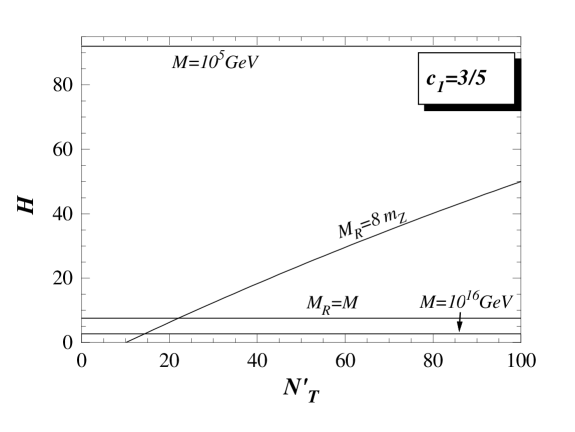
Figure 1:

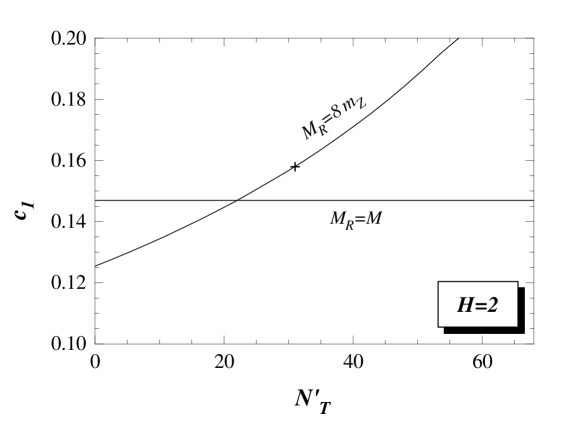
Figure 2:

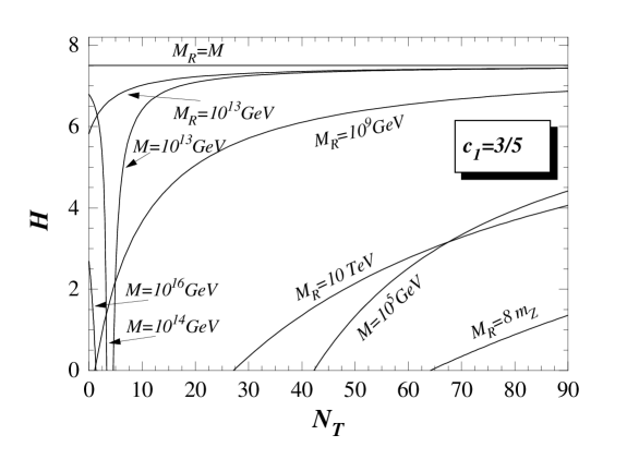
Figure 3:

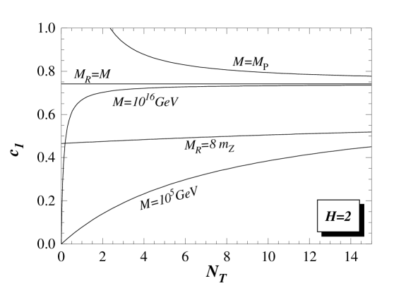
Figure 4:

References

- [1] U. Amaldi et al, Phys. Rev. D36, 1385 (1987).
- [2] H.Georgi and S.L. Glashow, Phys. Rev. Lett. 32, 438 (1974); H.Georgi, H.R.Quinn and S. Weinberg, Phys. Rev. Lett. 33, 451 (1974).
- [3] U.Amaldi, W. de Boer, and H. Furstenau, Phys. Lett B260, 447 (1991); P. Langacker and M. Luo, Phys. rev. D44, 817 (1991); U. Amaldi et al, Phys. Lett. B281, 374 (1992).
- [4] N.T.Shaban and W.J. Stirling, Phys, Lett. B291, 281 (1992).
- [5] H.Georgi, in Particles and Fields-1974, edited by C.E.Carlson (American Institute of Physics, NY, 1975), p. 575. H. Frietzsch and P. Minkowsky, Ann. Phys. 93, 193 (1975).
- [6] N.G.Deshpande, E.Keith and T.G.Rizzo, Phys. Rev. Lett. 70, 3189 (1993).
- [7] A.Pérez-Lorenzana, W.A. Ponce and A. Zepeda, Europhysics Lett. 39, 141 (1997).
- [8] A.Pérez-Lorenzana, W.A. Ponce and A. Zepeda, Mod. Phys. Lett. A13, 2153 (1998).
- [9] W. A. Bardeen, A. Buras, D. Duke and T. Muta, Phys. Rev. D18, 3998 (1978).
- [10] D. R. T. Jones, Phys. Rev. D15, 581 (1982). M. A. Machacek and M. T. Vaughn, Nucl. Phys. B222, 83 (1983).
- [11] Particle data Group: C. Caso et al, The Europhysics Journal C3 Nos. 1-4, 1 (1998).
- [12] The LEP Electroweak Working Group, LEPEWWG/97(02); J.Timmermans, Proceedings of LEP 97, Hamburg (1997); S.Dong, ibidem.
- [13] F.Gürsey, P.Ramond and P.Sikivie, Phys.Lett. B60, 177(1975); S.Okubo, Phys. Rev. D16, 3528 (1977).
- [14] A. de Rújula, H.Georgi, and S.L.Glashow, in Fifth Workshop on Grand Unification, edited by K.Kang, H.Fried, and P.Frampton (World Scientific, Singapore, 1984), p. 88; K.S.Babu, X-G. He, and S.Pakvasa, Phys. Rev. D33, 763 (1986).
- [15] F.Wilczek and A. Zee, Phys. Rev. D25, 553 (1982); J. Bagger et al., Nucl. Phys. B258, 565 (1985).
- [16] I.Bars and M. Gunaydin, Phys. Rev. Lett. 45, 859 (1980); S.M.Barr, Phys. Rev. D37, 204 (1988).
- [17] S.L.Adler, Phys. Lett. B225, 143 (1989); P.H.Frampton and B-H.Lee, Phys. Lett. 64,619 (1990); P.B.Pal, Phys. Rev. D43, 236 (1991); D45, 2566 (1992).
- [18] J.C.Pati, A.Salam, and J.Strathdee, Phys. Lett. 108B, 121 (1982); N.G.Deshpande, E.Keith, and P.B.Pal, Phys. Rev. D47, 2893 (1993).
- [19] N.G.Deshpande and P.Mannheim, Phys. Lett. 94B, 355 (1980); S.Day and M.K.Parida, Phys. Rev. D52, 518 (1995).
- [20] A. Davidson and K. C. Wali, Phys. Rev. Lett. 58, 2623 (1987); R. N. Mohapatra, Phys. Lett. B379, 115 (1996).
- [21] A.H.Galeana, R.Martínez, W.A.Ponce, and A.Zepeda, Phys. Rev. D44, 2166 (1991); W. A. Ponce, and A. Zepeda, Phys. Rev. D48, 240 (1993); J.B.Florez, W.A.Ponce, and A.Zepeda, Phys. Rev. D49, 4958 (1994).
- [22] J.C.Pati and A.Salam, Phys. Rev. Lett. 31,661 (1973); 36, 1229 (1976); Phys. Lett. 58B, 333 (1975); Phys. Rev. D8, 1240 (1973); D10, 275 (1974).
- [23] L. E. Ibáñez Phys. Lett.303B, 55 (1993). P. Ginsparg, Phys. Lett.197B, 139 (1987).
- [24] T. Appelquist and J. Carazzone, Phys. Rev. D11, 2856 (1975).
- [25] J.C.Pati and A.Salam, Phys. Rev. D10, 275 (1974); R.N.Mohapatra and J.C.Pati, Phys. Rev. D11, 566 (1974); D11, 2558 (1974); G. Senjanović and R.N.Mohapatra, Phys. Rev. D12, 1502 (1975).
- [26] F. del Aguila, and L. Ibañez, Nucl. Phys. B177, 60 (1981).
- [27] J.C.Pati and A.Salam, Nucl. Phys. B150, 76 (1979); P. H. Frampton and S. L. Glashow, Phys. Lett.190B, 157 (1987).
- [28] P.Cho, Phys. Rev. D48, 5331 (1993).
- [29] S.M.Barr and S.Raby, Phys. Rev. Lett. 79 4748(1997); C.H.Albright and S.M.Barr, Phys. Rev. D58, 013002 (1998).
- [30] T. Akagi et. al., Phys. Rev. Lett.67, 2614 (1991); ibid 67, 2618 (1991). A. M. Lee et. al., Phys. Rev. Lett.64, 165 (1990).
- [31] W.A.Ponce, and A.Zepeda, Z.Physik C63, 339 (1994); A.Pérez-Lorenzana, W.A.Ponce, and A.Zepeda: “Non-supersymmetric gauge coupling unification in[SU(6)] and proton stability, to appear in Rev. Mex. Fis.
- [32] R. Slansky, Phys. Reports, 79 No. 1, 1 (1981)
- [33] V.Elias and S. Rajpoot, Phys. Rev. D20, 2445 (1979).
- [34] F. Gürsey and P. Sikivie, Phys. Rev. Lett.36, 775 (1976); Phys. Rev. D16, 816 (1977). P. Ramond, Nucl. Phys. B110, 214 (1976); ibid B126, 509 (1977).