arch-ive/9812384 December 1998 UCB–PTH–98/59 LBNL–42574 SNS–PH/98–26 OUTP–98–86–P
Precise tests of a quark mass texture

Abstract

The relations $|V_{ub}/V_{cb}|=(m_{u}/m_{c})^{1/2}$ and $|V_{td}/V_{ts}|=(m_{d}/m_{s})^{1/2}$ between the CKM matrix elements and the quark masses are shown to imply a remarkably precise determination of the CKM unitarity triangle or of the Wolfenstein parameters $\rho$, $\eta$ consistent with the data so far. We view this as a clean test of a quark mass texture neatly arising from a hierarchical breaking of a U(2) flavour symmetry.

1 Introduction

The most striking omission in the current description of particle physics is a theory of fermion masses and mixings. In these respects, experiment is ahead of theory. All of the charged fermion masses are known, with a variable precision, as are known some of the mixing parameters in the quark sector. The knowledge of the quark mixing parameters should improve significantly and become perhaps complete in a near future, especially, but not only, due to $b$-physics experiments in various facilities. Related to this is the continuous effort to measure or put limits on all sorts of Flavour Changing Neutral Current processes. Even in the neutrino sector, remarkable experimental progress is being made which might ultimately lead to the determination of the neutrino masses and mixings as well. Theory, on the other hand, is so far mostly limited to a phenomenological approach, based on the studies of textures.

In this paper one such texture is considered and its experimental consequences spelled out in detail. Our motivations for doing this are twofold. On one side the texture that we consider is clearly motivated in an attempt to understand the flavour problem based on a spontaneously broken U(2) flavour symmetry [1, 2, 3, 4]. On the other side, the most constraining phenomenological relations that this texture implies are common to several different approaches to the quark flavour problem.

The texture we consider for the mass matrices of the $U$, $D$ quarks, $m_{U,D}$, up to irrelevant phase factors, is [4]

$$\left|\frac{m^{U,D}}{m^{U,D}_{33}}\right|=\begin{pmatrix}\ll{\epsilon^{\prime}}^{2}/\epsilon&\epsilon^{\prime}&\ll\epsilon^{\prime}\\ \epsilon^{\prime}&\epsilon&\mathcal{O}\left(\epsilon\right)\\ \ll\epsilon^{\prime}&\mathcal{O}\left(\epsilon\right)&1\end{pmatrix}$$ (1)

where $\epsilon^{\prime}\ll\epsilon\ll 1$ are parameters dependent on the quark charge.

It was shown in Refs [5, 3] that (1) implies the following form of the CKM matrix

$$V=\left(\begin{array}[]{ccc}c_{12}^{D}+s_{12}^{D}s_{12}^{U}e^{i\phi}&s_{12}^{D}-s_{12}^{U}e^{i\phi}&-s_{12}^{U}s\\ s_{12}^{U}-s_{12}^{D}e^{i\phi}&c_{12}^{D}e^{i\phi}+s_{12}^{U}s_{12}^{D}&s\\ s_{12}^{D}s&-c_{12}^{D}s&e^{-i\phi}\end{array}\right)$$ (2)

where

$$s_{12}^{D} =\sqrt{{m_{d}\over m_{s}}}\left(1-{m_{d}\over 2m_{s}}\right)$$ (3a)

$$c_{12}^{D} =\sqrt{1-(s_{12}^{D})^{2}}$$ (3b)

$$s_{12}^{U} =\sqrt{{m_{u}\over m_{c}}}$$ (3c)

or, in particular, [6]

$$\left|\frac{V_{ub}}{V_{cb}}\right| =\sqrt{\frac{m_{u}}{m_{c}}}$$ (4a)

$$\left|\frac{V_{td}}{V_{ts}}\right| =\sqrt{\frac{m_{d}}{m_{s}}}$$ (4b)

with $m_{u}$ and $m_{c}$, as $m_{d}$ and $m_{s}$, renormalized at the same scale. The further relation [7, 5]

$$V_{us}=s_{12}^{D}-s_{12}^{U}e^{i\phi}$$ (5)

is consistent with observation so far but it does not lead to a constraint on the CP-violating phase $\phi$ stronger than (1a,b) themselves together with the unitarity of the CKM matrix.

To be precise, Eqs (2,2) arise from an approximate diagonalization of (1) and have therefore corrections [3]. The biggest of such corrections is in $V_{ub}$ or in (1a). Its size, depending on the unknown order-1 coefficients in the 23 and 32 elements of (1), can range up to 10%, whereas all other corrections are below 2–3%. For this reason, a 10% random correction to (1a) is included in the following considerations.

In Section 2 we show that Eqs (1a,b) give a remarkably precise determination of the standard CKM unitarity triangle or, in the commonly used Wolfenstein parameterization [8], of the parameters $\rho,\eta$. In turn, as made explicit in Sects 3, 4, this should allow a clear comparison of these predictions with forthcoming experimental results.

As mentioned, to the extent that Sects 2–4 are only based on Eqs (1a,b), this analysis serves a broader scope than the determination of the U(2)-predictions themselves. In particular it applies to all flavour models that have (1) as their starting point. A comparison of Eqs (1a,b) with present data has also been made in ref [9]. This reference treats differently the information on the light quark mass ratios, it does not attribute a theoretical error to Eq (1a) and it uses a different parametrization of the CKM matrix [3, 10].

2 Constraint in the $\rho$-$\eta$ plane

In Eqs (1,5), the ratios of light quark masses $m_{u}/m_{d}$, $m_{d}/m_{s}$, $m_{u}/m_{c}$ are involved. In our analysis we use $m_{u}/m_{d}$ and the combination [11]

$$Q=\frac{m_{s}/m_{d}}{\sqrt{1-(m_{u}/m_{d})^{2}}}$$ (6)

rather than $m_{u}/m_{d}$ and $m_{d}/m_{s}$. The reason is that chiral perturbation theory determines $Q$ to a remarkably accuracy whereas additional assumptions, plausible but not following from pure QCD, are required to determine $m_{u}/m_{d}$. It turns out that $Q$ alone allows to restrict the range of $\rho$, $\eta$ in a significant way. Relations (1 a,b) allow to express $Q$, $m_{u}/m_{d}$, $m_{c}/m_{s}$ in terms of ${\bar{\rho}}$, ${\bar{\eta}}$, $m_{c}/m_{s}$. $\rho$, $\eta$, $A$, $\lambda$ are the Wolfenstein parameters and ${\bar{\rho}}=c\rho$, ${\bar{\eta}}=c\eta$, where $c=\sqrt{1-\lambda^{2}}$. We have in fact on one hand

$$\left|\frac{V_{ub}}{V_{cb}}\right| =\frac{\lambda}{c}\sqrt{{\bar{\rho}}^{2}+{\bar{\eta}}^{2}}$$ (7a)

$$\left|\frac{V_{td}}{V_{ts}}\right| =\frac{\lambda}{c}\sqrt{(1-{\bar{\rho}})^{2}+{\bar{\eta}}^{2}}$$ (7b)

(the last one with a 2% $\lambda^{2}$ correction suppressed) and, on the other hand,

$$\frac{m_{u}}{m_{c}}=\frac{m_{u}}{m_{d}}\frac{m_{d}}{m_{s}}\frac{m_{s}}{m_{c}}=\frac{m_{u}/m_{d}}{Q\sqrt{1-(m_{u}/m_{d})^{2}}}\frac{m_{s}}{m_{c}},$$ (8a)

$$\frac{m_{d}}{m_{s}}=\frac{1}{Q\sqrt{1-(m_{u}/m_{d})^{2}}}.$$ (8b)

Therefore we get, from (1a) and (1b) respectively

$$({\bar{\rho}}^{2}+{\bar{\eta}}^{2})=\frac{c^{2}}{\lambda^{2}Q\sqrt{1-(m_{u}/m_{d})^{2}}}\frac{m_{s}}{m_{c}}\frac{m_{u}}{m_{d}}$$ (9a)

$$(1-{\bar{\rho}})^{2}+{\bar{\eta}}^{2}=\frac{c^{2}}{\lambda^{2}Q\sqrt{1-(m_{u}/m_{d})^{2}}}.$$ (9b)

The random correction to (1a), at most of 10%, can be taken into account by attributing an effective extra error to $m_{c}/m_{s}$ appearing in (2a) of about 20%, included in the following considerations.

From Eqs (2), using the inputs in Table 1 we fit the parameters ${\bar{\rho}}$, ${\bar{\eta}}$. The result of the fit is shown in Fig (1) (small regions).

$$\begin{array}[]{|c|c|}\hline\cr Q&22.7\pm 0.8\\ m_{u}/m_{d}&0.553\pm 0.043\\ m_{c}/m_{s}&8.23\pm 1.5\\ \hline\cr\end{array}$$

Table 1: Input values for the quark mass ratios. $Q$ is defined in the text.

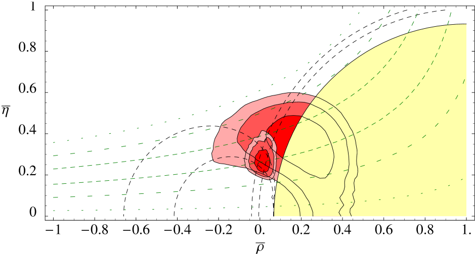
Figure 1: Fit 1 (smaller regions): Predictions for $\rho$, $\eta$ using Eqs (1) and the inputs in Table 1. Also shown are the two individual constraints (2b), (2c) separately (see text). Fit 2 (larger regions): SM fit using $|V_{ub}/V_{cb}|$, $\Delta m_{B_{d}}$, $\Delta m_{B_{s}}$ but not $\epsilon_{K}$, whose constraint is shown independently with different theoretical errors (see text). For both fits the contours are at 68, 95 and 99% CL respectively.

By combining (2a) and (2b), it is possible to eliminate $m_{u}/m_{d}$, whose value may not be reliably known, to obtain

$$\left((1-{\bar{\rho}})^{2}+{\bar{\eta}}^{2}\right)^{2}-\left(\frac{m_{c}}{m_{s}}\right)^{2}({\bar{\rho}}^{2}+{\bar{\eta}}^{2})^{2}=\frac{c^{4}}{\lambda^{4}Q^{2}}.$$ (9a)

Fig (1) also shows separately the constraints (2b) and (2c). The first is a circumference in the ${\bar{\rho}}$-${\bar{\eta}}$ plane centered at $({\bar{\rho}},{\bar{\eta}})=(1,0)$. The region plotted corresponds to the variation of the right hand side of (2b) within its $1\sigma$ error. Also shown is the region excluded by $m_{u}/m_{d}\geq 0$. The second constraint, (2c), corresponds to the two approximate half-circumferences around the origin meeting on the positive ${\bar{\rho}}$ axes. In drawing this constraint we allow $m_{c}/m_{s}$ to vary within its 68% error.

Note that Eqs (2a,b) are invariant under ${\bar{\eta}}\rightarrow-{\bar{\eta}}$, so that a complete Fig 1 would have to include a symmetric negative ${\bar{\eta}}$-region.

3 Comparison with present data

This prediction of $\rho,\eta$ can be compared with the usual determination, in a Standard Model fit, of these same parameters. The inputs for this last determination include the direct measurement of $|V_{ub}/V_{cb}|$ and the indirect information from the CP-violating parameter, $\epsilon_{K}$, the mixing in the $B_{d}$-system, $\Delta m_{B_{d}}$, and in the $B_{s}$ system, $\Delta m_{B_{s}}$. We prefer not to include in the SM fit the parameter $\epsilon_{K}$ since we leave open the possibility that some extra sources of CP-violation not included in the SM may exist, affecting in particular CP-violation in the Kaon system.

For ease of the reader we summarize the (standard) procedure of the SM fit, whose result is also plotted in Fig 1 (larger regions). The formulae used are

$$\left|\frac{V_{ub}}{V_{cb}}\right|=\frac{\lambda}{c}\sqrt{{\bar{\rho}}^{2}+{\bar{\eta}}^{2}}$$ (10a)

$$\Delta m_{B_{d}}=\frac{G_{F}^{2}}{6\pi}M_{W}^{2}|V_{td}|^{2}m_{B_{d}}\left(f_{B_{d}}\sqrt{B_{B_{d}}}\right)^{2}\eta_{B}\,x_{t}S(x_{t})$$ (10b)

$$\Delta m_{B_{s}}=\Delta m_{B_{d}}\frac{m_{B_{s}}}{m_{B_{d}}}\zeta^{2}\left|\frac{V_{ts}}{V_{td}}\right|^{2},$$ (10c)

where $|V_{td}|=\lambda^{3}A\,|1-{\bar{\rho}}-i{\bar{\eta}}|$, $|V_{ts}|=A\lambda^{2}c|1+\lambda^{2}({\bar{\rho}}+i{\bar{\eta}})|$, $\zeta=(f_{B_{s}}\sqrt{B_{B_{s}}})/(f_{B_{d}}\sqrt{B_{B_{d}}})$,

$$S(x_{t})=x_{t}\left(\frac{1}{4}+\frac{9}{4(1-x_{t})}-\frac{3}{2(1-x_{t})^{2}}-\frac{3\,x_{t}^{2}\log(x_{t})}{2(1-x_{t})^{3}}\right),$$

$x_{t}=m_{t}^{2}/M_{W}^{2}$ and the numerical values of the parameters are listed in Table 2 (in the RHS of (3c) $\Delta m_{B_{d}}$ is an experimental input). The parameters without error in Table 2 have not been varied in the fit. The remaining ones are quoted with their 68% error. They are both experimental inputs and fit variables, hence they have been integrated from the fit by choosing them in a random way (assuming gaussian distribution). The limit on $\Delta m_{B_{s}}$ has been implemented using the full set of data in the context of the “amplitude method”, provided by the Oscillation Working Group [12]. The data correspond to the recent limit $\Delta m_{B_{s}}>12.4\,\text{ps}^{-1}$ at 95% C.L. For a given value of $\Delta m_{B_{s}}$ as given by (3c), the corresponding amplitude $a(\Delta m_{B_{s}})$ with its error $\sigma_{a}(\Delta m_{B_{s}})$ is recovered from the data in [12], then $a(\Delta m_{B_{s}})$ is compared with 1, the value corresponding to a pure oscillation. The multiplicative contribution to the probability density from $\Delta m_{B_{s}}$ is then $\text{Exp}(-(a(\Delta m_{B_{s}})-1)^{2}/(2\sigma^{2}_{a}(\Delta m_{B_{s}}))$.

$$\begin{array}[]{||c|c||c|c||}\hline\cr G_{F}&1.16639\cdot 10^{-5}\,\mathrm{GeV}^{-2}&M_{W}&80.375\\ \lambda&0.2196&A&0.819\pm 0.035\\ m_{B_{d}}&(5.2792\pm 0.0018)\,\mathrm{GeV}&m_{B_{s}}&(5.3692\pm 0.0020)\,\mathrm{GeV}\\ f_{B_{d}}\sqrt{B_{B_{d}}}&(0.201\pm 0.042)\,\mathrm{GeV}&\zeta&1.14\pm 0.08\\ \eta_{B}&0.55\pm 0.01&m_{t}&(166.8\pm 5.3)\,\mathrm{GeV}\\ \Delta m_{B_{d}}&(0.471\pm 0.016)\text{ps}^{-1}&\epsilon_{K}&(2.280\pm 0.019)\cdot 10^{-3}\\ B_{K}&0.87\pm 0.14&f_{K}&(0.1598\pm 0.0015)\,\mathrm{GeV}\\ m_{K}&(0.497672\pm 0.000031)\,\mathrm{GeV}&\Delta m_{K}&(3.491\pm 0.009)\cdot 10^{-12}\,\mathrm{MeV}\\ \eta_{1}&1.38\pm 0.53&\eta_{2}&0.574\pm 0.004\\ \eta_{3}&0.47\pm 0.04&|V_{ub}/V_{cb}|&0.093\pm 0.016\\ \hline\cr\end{array}$$

Table 2: Inputs for the SM fit.

Figure 1 shows consistency between the prediction of the ${\bar{\rho}},{\bar{\eta}}$ parameters and their present determination in the SM. The figure also shows that the constraint (2c) alone, with the $Q$ input but without $m_{u}/m_{d}$, reduces considerably the allowed region. In fact, a combined fit of $|V_{ub}/V_{cb}|$, $\Delta m_{B_{d}}$, $\Delta m_{B_{s}}$ and (2c) gives as an output $m_{u}/m_{d}=0.61^{+0.13}_{-0.16}$.

The inclusion of $\epsilon_{K}$ in the SM fit would not alter the agreement between the predicted ${\bar{\rho}}$, ${\bar{\eta}}$ and present data. To see this, the constraint given by $\epsilon_{K}$ is shown independently in Fig. 1, where the regions allowed by a SM contribution to $\epsilon_{K}$ in some ranges around the central experimental value are plotted. More precisely, the constraint is given by

$$\frac{\epsilon_{K}}{C_{\epsilon}B_{K}A^{2}\lambda^{6}}={\bar{\eta}}\left(-\eta_{1}S(x_{c})+\eta_{3}S(x_{c},x_{t})+A^{2}\lambda^{4}(1-{\bar{\rho}}+\lambda^{2}({\bar{\rho}}(1-{\bar{\rho}})-{\bar{\eta}}^{2}))\eta_{2}S(x_{t})\right),$$ (11)

where

$$S(x_{c},x_{t})=x_{c}\left(\log\frac{x_{t}}{x_{c}}-\frac{3x_{t}}{4(1-x_{t})}-\frac{3x_{t}^{2}\log x_{t}}{4(1-x_{t})^{2}}\right),$$

$$C_{\epsilon}=\frac{G_{F}^{2}f_{K}^{2}m_{K}M_{W}^{2}}{6\sqrt{2}\pi^{2}\Delta m_{K}}.$$

The values we used for the parameters are also listed in Table 2 with their errors. On the RHS in (11) only the central values have been used, that is enough for our purposes. The LHS has a 68% error mostly coming from the denominator. The 3 regions shown in Fig. 1 correspond to three different ranges for the LHS all in the form $\text{LHS}\pm(68\%\text{ error on LHS)}\pm\text{(extra error)}$, where the “extra error” is 0, 1/3, 2/3 of the LHS in the three regions respectively. The extra error takes into account the possibility of contributions to $\epsilon_{K}$ from non-SM physics. The figure shows that models in which relations (1) are valid do not require large corrections to the SM value.

4 Potential improvements of the comparison with data

The prospects for an improved comparison of the predictions of the texture (1) with further data are clear from Fig 1. Another way to illustrate this is in Fig (2). Shown there are the probability distributions for $\rho,\eta$ and for various physical quantities obtained by a combined fit of $|V_{ub}/V_{cb}|$, $\Delta m_{B_{d}}$, $\Delta m_{B_{s}}$ and the constraints (1). These distributions are compared with those from a pure SM fit with present data and $\epsilon_{K}$ still not included, but rather shown as an output (Fig 2d). As noted above, the sign of $\eta$ is not fixed by Eqs (2) nor it is determined in the SM fit, since $\epsilon_{K}$ is not included. As such, the probability distributions in Figs 2a,b,d,h, drown for $\eta>0$, must be reflected around the origin of their orizontal axis for the $\eta<0$ case. Based on this figure one can be optimistic on the possibility of a stringent comparison with data to come.

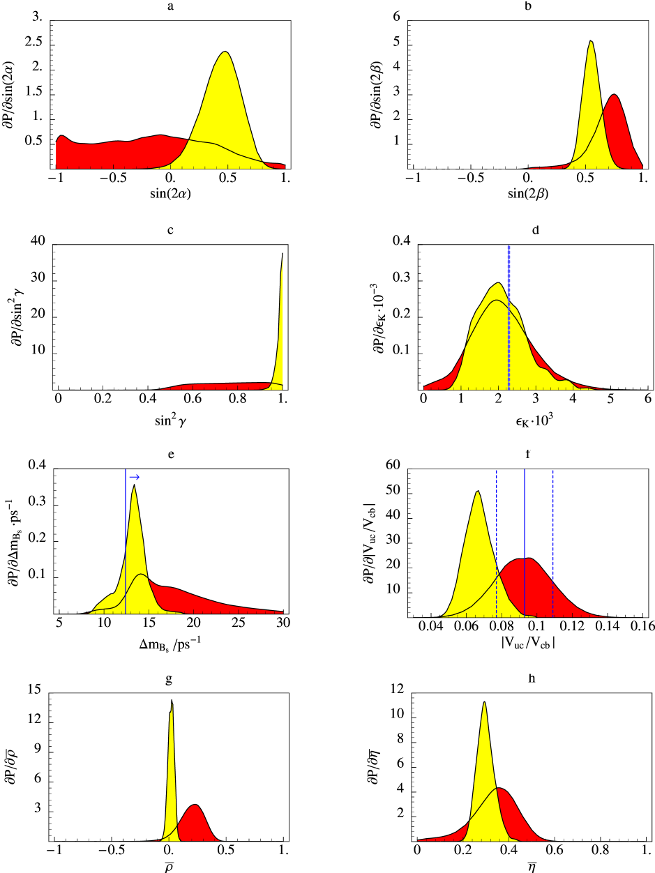
Figure 2: Probability distributions (lighter area: predictions; darker area: from the SM fit, excluding $\epsilon_{K}$ but taking $\eta>0$) for different observables: a) $\sin 2\alpha$, b) $\sin 2\beta$, c) $\sin^{2}\gamma$, d) $\epsilon_{K}$, e) $\Delta m_{B_{s}}$, f) $\zeta$, g) $\rho$, h) $\eta$.

It is less clear, in fact, that an improvement may come from an independent better determination of the inputs in Table 1. On the contrary, one has to keep in mind, as repeatedly stressed, that the theoretical determination of $m_{u}/m_{d}$ is not on the same ground as for the two other parameters. For this reason the prediction for various physical observables is shown in Fig 3 as function of $m_{u}/m_{d}$ and $\eta>0$. Since some of these observables have a significant dependence on this ratio, with better data it would be useful to leave even $m_{u}/m_{d}$ as a free parameter. Notice in Fig 2f the preferred value of $|V_{ub}/V_{cb}|$ relative to the present determination, mostly affected by theoretical uncertainties. Notice also in Figs 2e and 3e the critical lower bound on $\Delta m_{B_{s}}$.

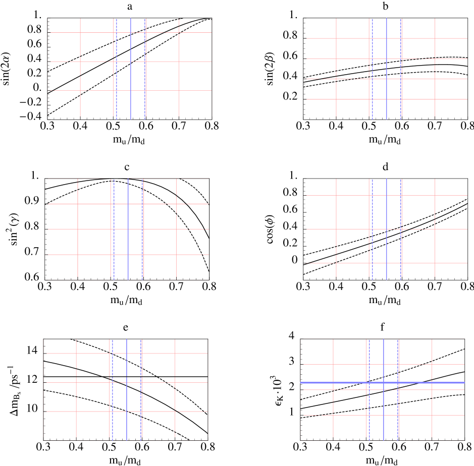
Figure 3: Predictions as functions of $m_{u}/m_{d}$ for different observables: a) $\sin 2\alpha$, b) $\sin 2\beta$, c) $\sin^{2}\gamma$, d) $\cos\phi$, e) $\Delta m_{B_{s}}$, f) $\epsilon_{K}$.

5 Conclusions

The quark mass matrix texture of equation (1) provides a simple structure of hierarchical masses and nearest neighbour mixing. It is an immediate consequence of a hierarchical breaking of a U(2) flavour symmetry. On diagonalizing the up and down quark matrices with this texture, one discovers that the 12 rotations determine both the ratio of the smaller eigenvalues and the size of 13 mixing relative to 23 mixing: $|V_{ub}/V_{cb}|=(m_{u}/m_{c})^{1/2}$ and $|V_{td}/V_{ts}|=(m_{d}/m_{s})^{1/2}$. These relations arise in any scheme of hierarchical quark masses where the 11, 13 and 31 entries are sufficiently small, and the 12 and 21 entries are equal up to a phase. Using the Wolfenstein form for the CKM matrix, we have shown that these two relations can be translated into a tight prediction in the ${\bar{\rho}}$-${\bar{\eta}}$ plane. The predicted region is significantly smaller than that currently allowed by data, as shown in Figure 1: the texture successfully accounts for the present data and will be subject to further stringent tests by future data.

The most important implications for future experiments are: a deviation from complete $B_{s}$ mixing must be discovered soon, $\Delta m_{B_{s}}<14.9\,\text{ps}^{-1}$ at 90% c.l., and the predicted probability distributions for $|\sin 2\alpha|$ and $|\sin 2\beta|$ are both peaked near 0.5, as shown in Figures 2a,b,e. These results use $m_{u}/m_{d}=0.55\pm 0.04$ as an input. However, even if this input is completely relaxed, so that only one combination of the two light mass ratios is used, the upper bound on $B_{s}$ mixing remains robust: $\Delta m_{B_{s}}<15\,\text{ps}^{-1}$ at 90% c.l. In this case significant variations in $\sin 2\alpha$ and $\sin 2\beta$ are possible, as shown in Figures 3a,b. Note in any case that lower values of $m_{u}/m_{d}$, that could accommodate a higher $\Delta m_{B_{s}}$, push further down the expected value of $|V_{ub}/V_{cb}|$, in apparent contradiction with the present determination.

These results are all independent of whether there is a significant non-standard model contribution to $\epsilon_{K}$. However, the size of such an exotic contribution is restricted by the form of the texture, as shown in Figure 3f. In the absence of such a contribution, the combination of Figures 3e and 3f predicts that $m_{u}/m_{d}$ is not far from the commonly accepted value of $0.55\pm 0.04$.

References

- [1] A. Pomarol and D. Tommasini, Nucl. Phys. B466, 3 (1996).
- [2] R. Barbieri, G. Dvali, and L. J. Hall, Phys. Lett. B377, 76 (1996).
- [3] R. Barbieri, L. J. Hall, and A. Romanino, Phys. Lett. B401, 47 (1997).
- [4] R. Barbieri, L. Giusti, L. J. Hall, and A. Romanino, Fermion masses and symmetry breaking of a U(2) flavour symmetry, hep-ph/9812239.
- [5] L. J. Hall and A. Rasin, Phys. Lett. B315, 164 (1993).
-
[6]
H. Fritzsch,
Nucl. Phys. B155, 189 (1979).
B. Stech, Phys. Lett. 130B, 189 (1983). -
[7]
H. Fritzsch,
Phys. Lett. B73, 317 (1978);
M. Shin, Phys. Lett. B145, 285 (1984);
M. Gronau, R. Johnson and J. Schechter, Phys. Rev. Lett. 54, 2176 (1985). - [8] L. Wolfenstein, Phys. Rev. Lett. 51, 1945 (1983).
- [9] F. Parodi, P. Roudeau and A. Stocchi, Constraints on the parameters of the matrix at the end of 1997, preprint LAL 98–49, hep-ph/9802289.
- [10] H. Fritzsch and Z. Xing, Phys. Lett. B413, 396 (1997).
- [11] H. Leutwyler, The masses of the light quarks, Talk given at the Conference on Fundamental Interactions of Elementary Particles, ITEP, Moscow, Russia, 1995, hep-ph/9602255.
- [12] The LEP B Oscillation Working Group ”Combined Results on Oscillations: Update for Summer 1998 Conferences”, LEPBOSC 98/3.