hep-ph/9812382
RM3-TH/99-3

Recent developments in deep-inelastic scattering

Stefano Forte
INFN, Sezione di Roma III
Via della Vasca Navale 84, I-00146, Roma, Italy

We review several recent developments in the theory and phenomenology of deep-inelastic scattering, with particular emphasis on precision tests of QCD and progress in the detailed perturbative treatment of structure functions and parton distributions. We discuss specifically determinations of $\alpha_{s}$; higher twist contributions to structure functions and renormalons; structure functions at small $x$ and resummation of energy logarithms.

July 1999

1 DIS in the collider age

Deep-Inelastic Scattering (DIS) is the traditional testing ground of perturbative QCD. In the last several years, perturbative QCD has become, as an integral part of the standard model, a firmly established theory, which allows performing detailed and reliable calculations. Current work is focussed on the precise determinations of the unknown parameters of the theory, and the development of reliable computational techniques. The parameters to be determined include not only the strong coupling $\alpha_{s}$, which is the only free parameter in the QCD Lagrangian, but also all quantities which are determined from the nonperturbative low–energy dynamics, and thus, even though in principle computable, must in practice be treated as a phenomenological input in the perturbative domain.

In the case of DIS, the low–energy parameters are the parton distributions of hadrons. Thanks to the operator-product expansion and the renormalization group, or more in general factorization theorems, the coefficient functions which relate parton distributions to measurable cross-sections can be computed in perturbation theory. Furthermore, the scaling violations of the parton distributions are related to the short–distance behavior of local operators in the theory, and can thus also be computed reliably. Deep-inelastic scattering provides therefore the most accurate way of determining the parton distributions which are then used as an input in the perturbative computation of hard processes relevant for collider physics, as well as, through scaling violations, one of the prime ways of determining $\alpha_{s}$.

In recent times, the status of the DIS phenomenology has changed substantially, largely due to the advent of the HERA lepton-hadron collider, which has enormously enlarged the kinematic coverage of the data. In the simplest fully inclusive case, the DIS kinematics is fully parametrized by the virtuality $Q^{2}$ of the photon which mediates the lepton-hadron process, and the total center-of-mass energy

$$W^{2}=Q^{2}{1-x\over x}$$ (1)

of the virtual photon-hadron process (which implicitly defines the Bjorken variable $x$). By definition, the DIS region correspond to large $Q^{2}$; the accessible values of $x$ are then limited by the available energy. HERA has thus opened up a large previously unaccessible region in the $(x,Q^{2})$ plane. However, some very interesting complementary information has also been obtained recently by fixed-target experiments, which have provided high-statistics data especially in the polarized case, in neutrino scattering experiments, and in charged lepton scattering in the large $x$ region, where $W^{2}$ is low on the scale of $Q^{2}$.

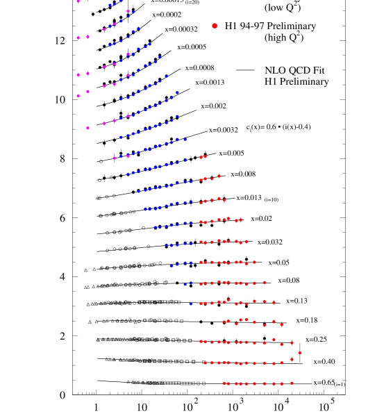
Figure 1: The proton structure function $F_{2}(x,Q^{2})$ measured by the H1 collaboration at HERA as well as by SLAC[5], BCDMS[3] and NMC[4] fixed-target experiments (from Ref.[6]).

The current state of the art can be inferred from Fig. 1, which displays the data on the inclusive structure function $F_{2}(x,Q^{2})$ collected by one of the HERA collaborations between 1994-1997, as well as earlier fixed-target data. The data are compared to the behavior expected by solving the Altarelli-Parisi evolution equations to next-to-leading order (NLO), with a fixed value of the strong coupling $\alpha_{s}(M_{z})=0.118$. Parton distributions are parametrized at a fixed initial scale $Q_{0}^{2}=2$ GeV² with a dozen free parameters, fitted by comparing to the data. It is apparent that despite the enormous magnification of kinematic coverage, there is perfect agreement between the data and the QCD prediction, and the agreement does not seem to deteriorate even when approaching regions where the NLO computation might be expected to be not entirely adequate. In particular, no signs of deviation from the NLO QCD prediction are seen in the small $x$ region, which was unexplored before HERA.

It is important to understand what is and what is not remarkable about the agreement of data and theory displayed in Figure 1. The fact that it is possible to achieve a good description of a large number of data with relatively few parameters is not especially interesting per se: it may simply indicate that the functional dependence of the data on the kinematic variables is sufficiently smooth.

In fact, there exist parameterizations of $F_{2}(x,Q^{2})$, constructed by experimental collaborations for the purpose of data analysis, which interpolate all available data [7]. These parameterizations do not use perturbative QCD at all: they simply fit a functional form to the data, yet they hardly need a larger number of free parameters. Furthermore, several recent parameterizations of $F_{2}$ at low $Q^{2}$ (where perturbative evolution is not valid), derived within various non-perturbative low energy models[8] appear to give a reasonably good description of the $F_{2}$ data (though generally not quite as accurate as the QCD calculation) even up to values of $Q^{2}$ as large as 100 GeV², where perturbative QCD should be used instead. Conversely, a recent phenomenological parameterization[9], inspired by a linearization of the perturbative QCD prediction, describes the low $x$ and large $Q^{2}$ data with only 4 parameters, and turns out to work very well even when $Q^{2}$ is as low as 0.05 GeV², where the perturbative approach is certainly invalid.

It would be equally unreasonable to take the latter as evidence of the validity of perturbation theory at very low $Q^{2}$, or the former as evidence that at large $Q^{2}$ perturbative QCD should be replaced by nonperturbative models: what distinguishes a perturbative computation such as the one shown in Figure 1 is its predictive power. Namely, the data are parametrized as a function of $x$ at a reference scale $Q_{0}^{2}$, and increasing the number of parameters only results in a more accurate description of the $x$ dependence of the data at that scale. The structure function at any other scale is then predicted, by solving the evolution equations. This is to be contrasted with the situation in a fit, whether or not inspired by a theoretical model. There, no prediction is available: the $x$ and $Q^{2}$ dependence are fitted in a certain kinematic domain, and then extrapolated outside it.

The extraordinary success of the perturbative prediction displayed in Fig. 1 reflects the fact that the meaning of a “test of QCD” has changed in the last decade. The correctness and consistency of the theory are no longer at stake: tests of its parameter-free predictions (such as the Bjorken sum rule [10], Sect 2.2, or the small $x$ slope [11], Sect.2.3) are impressively succesful. The phenomenological emphasis is now on precision determination of parameters which must be used as input for the reliable calculation of hadron collider processes, and as backgrounds to possible new physics. As an example of this, we will discuss in Sect. 2 the determination of $\alpha_{s}$, where the agreement of values extracted from different experiments is now taken for granted, and the aim of current work is to obtain an accurate value of $\alpha_{s}$ for use in the computation of standard model processes. On the other hand, “testing” the theory has taken the meaning of stretching the usual perturbative techniques based on hard factorization. This can be done moving towards regions of lower scale, where power corrections are important, as we will discuss in Sect. 3 with specific reference to DIS at large $x$. It can also be done by studying regions where more than one hard scale is present, as we will discuss in Sect. 4 in the case of small $x$ evolution. An altogether different possibility is to stretch the domain of factorization theorem to less inclusive phenomena. Specifically, recent data at HERA (and elsewhere) have greatly extended our knowledge of lepton-hadron scattering in the diffractive region, both within and outside the deep-inelastic domain. A discussion of this topic[12] is however outside the scope of this review.

2 Determinations of $\alpha_{s}$

A glance to the current edition of the particle data book[15] shows that a sizable part of our knowledge of $\alpha_{s}$ comes from DIS, and specifically from scaling violations. Even though this kind of determination of $\alpha_{s}$ does not have nominally the smallest uncertainty, it is, together with the determination from the $Z$ width, the most reliable from a theoretical viewpoint. The main recent progress here, in comparison for instance to the previous edition[16] of the particle data book, consists of the fact that, even though the experimental uncertainty has been only marginally reduced, the central value of $\alpha_{s}(M_{z})$ is now in significantly better agreement with the world average, and with the value obtained from LEP data. This is partly due to the fact that some pieces of data had experimental problems which have now been corrected, partly due to the fact that some sources of theoretical uncertainty hadn’t been appreciated fully, and partly to the availability of new data. Here, we will review recent advances in the extraction of $\alpha_{s}$ from inclusive structure function data. Of course, $\alpha_{s}$ can also be extracted from jet rates and event shapes. These determinations, which are only possible at large center-of-mass energy, in the lepton-hadron case have first become possible at HERA; they are however still in their infancy and not yet competitive with inclusive determinations[17]

2.1 Scaling violations of structure functions

The scaling violations of the structure functions $F_{2}$ and $F_{3}$ (unpolarized) and $g_{1}$ (polarized) are driven by the value of $\alpha_{s}$ according to

$${d\over dt}F_{2}(N,Q^{2}) = {\alpha_{s}(Q^{2})\over 2\pi}\left[\gamma_{NS}(N)F_{2}^{\rm nonsing.}+\gamma_{qq}(N)F_{2}^{\rm sing.}\right.$$

$$\quad\left.\phantom{g_{1}^{\rm nonsing.}}+2c\,n_{f}\gamma_{qg}(N)g(N,Q^{2})\right]+O(\alpha_{s}^{2})$$

$${d\over dt}F_{3}(N,Q^{2}) = {\alpha_{s}(Q^{2})\over 2\pi}\gamma_{NS}(N)F_{3}+O(\alpha_{s}^{2})$$ (2)

$${d\over dt}g_{1}(N,Q^{2}) = {\alpha_{s}(Q^{2})\over 2\pi}\left[\Delta\gamma_{NS}(N)g_{1}^{\rm nonsing.}+\Delta\gamma_{qq}(N)g_{1}^{\rm sing.}\right.$$ (3)

$$\quad\left.\phantom{g_{1}^{\rm nonsing.}}+c\,n_{f}\Delta\gamma_{qg}(N)\Delta g(N,Q^{2})\right]+O(\alpha_{s}^{2}),$$

where $F_{2}(N,Q^{2})\equiv\int_{0}^{1}\,dxx^{N-1}F_{2}(x,Q^{2})$ is the $N$–th Mellin moment of the function $F_{2}(x,Q^{2})$, $g$ and $\Delta g$ are the unpolarized and polarized gluon distributions, the anomalous dimensions $\gamma(N)$ are the Mellin transforms of the Altarelli-Parisi splitting functions $P(x)$, and the factor $c={1\over n_{f}}\sum_{i=1}^{n_{f}}e^{2}_{i}$ for charged lepton and $c=1$ for neutrino scattering. In order to extract $\alpha_{s}$ we need thus either to be able to separate out the nonsinglet component of $F_{2}$, or to disentangle the singlet, nonsinglet and gluon distribution, or to determine the parity violating structure function $F_{3}$ (which only contributes to neutrino DIS). Knowledge of the next-to-leading order corrections to eq. (3) allows then to fix the scale at which $\alpha_{s}$ is evaluated.

The current[15] global average value of $\alpha_{s}$ from unpolarized scaling violations is $\alpha_{s}(M_{z})=0.117\pm 0.002({\rm exp.})\pm 0.004({\rm th.})$. This average includes results from global analyses of electron[18], muon[19] and neutrino[20] DIS data, i.e. obtained by introducing a parameterization of the singlet, nonsinglet and gluon at a reference scale, evolving it up to the values of $Q^{2}$ at which data are available, and inverting the Mellin transform in order to compare the structure function $f(x,Q^{2})$ to the data. In all analyses included in the above average, computations (and specifically the solution of the evolution equations) are performed to next-to-leading order (NLO).

The current value is to be contrasted with the earlier[16] value $\alpha_{s}(M_{z})=0.112\pm 0.002({\rm exp.})\pm 0.004({\rm th.})$. The central value has gone up because of a re-evaluation of the CCFR result from neutrino scattering, which now gives[20] $\alpha_{s}(M_{z})=0.119\pm 0.002({\rm exp.})\pm 0.004({\rm th.})$ (the previous central value was[21] $\alpha_{s}(M_{z})=0.111\pm 0.002({\rm exp.})\pm 0.003({\rm th.})$). The variation is mostly due to a re-calibration of the energy of the neutrino beam along with smaller improvements and corrections. Because of the smallness of its error, the CCFR determination now dominates the value of $\alpha_{s}$ from scaling violations, and we will thus discuss it in some detail.

The peculiarity of the CCFR determination of $\alpha_{s}$ which justifies its small statistical error is the fact that the use of a neutrino beam allows a simultaneous determination of the structure functions $F_{2}$ and $F_{3}$, and thus a reliable separation of the singlet and nonsinglet components. The range of $Q^{2}$ covered by the data is reasonably high, $5\leq Q^{2}\leq 125$ GeV², and an estimate of the error associated to power corrections is included.

A shortcoming of the analysis, however, is the relatively crude form of the parton parameterization adopted: no attempt is made to fit the detailed $x$ shape of the structure function; this may lead to an underestimate of the systematic error.[10] A perhaps more interesting potential source of trouble is related to higher order corrections, whose impact was not studied (the corresponding error is assumed to be the same as determined in the unrelated analysis of ref.[3]).

In fact, the NNLO anomalous dimensions have been recently determined, at least for even integer values of $2\leq N\leq 10$.[22] Since the large $N$ (see Sect. 3) and small $N$ (see Sect. 4) behavior of the anomalous dimensions is also known, it is possible to reconstruct approximately the full anomalous dimension by interpolation. A NNLO analysis can then be attempted. The CCFR $F_{3}$ (i.e. pure nonsinglet) data have been recently reanalyzed in this way. [23, 24] The inclusion of NNLO terms results in a decrease of the $\chi^{2}$ (by about 5 units with about 10 d.o.f.), and in a lower central value of $\alpha_{s}$ by $\delta\alpha_{s}(M_{z})=0.004$. Since this is equal to the total theoretical error quoted in ref.[20], it suggests that this error may actually be underestimated; a careful inclusion of other sources of theoretical uncertainty (specifically related to heavy quark thresholds) suggests that a more realistic estimate might be $\Delta[{\rm th.,NLO}]\alpha_{s}(M_{z})=0.006$, which at NNLO is reduced to $\Delta[{\rm th.,NNLO}]\alpha_{s}(M_{z})=0.003$ (these numbers apply to the pure nonsinglet analysis of ref.[23]). An alternative NNLO determination from “world” data [25] finds $\alpha_{s}(M_{z})=0.1163\pm 0.0016({\rm exp.})\pm 0.0016({\rm th.})$. Here, the smaller statistical error is due to using a wider dataset, while the smaller theory error comes from a less conservative treatment of theoretical errors: a less general parameterization of higher twists is used, and higher orders are estimated by different linearization of the Altarelli-Parisi solution rather than by scale variation.

Another important potential source of error is related to the inclusion of contributions to the evolution equations beyond logarithmic accuracy, i.e. corrections to eq. (3) suppressed by powers of $Q^{2}$ (higher twist corrections). We will discuss this issue in detail in Sect. 3. In ref.[20] an estimate of higher twist corrections is included on the basis of a renormalon model (see Sect. 3.1), and assigned a 100% error, which gives an uncertainty $\Delta({\rm HT,NLO})\alpha_{s}(M_{z})=0.001$. A (much) more conservative estimate is obtained by parameterizing the higher twist corrections by a function $h(x)\over Q^{2}$ which is left as an extra free parameter for each $x$ data bin in the fit. In such case the theory error is enormously increased to[23] $\Delta({\rm th.+HT,NLO})\alpha_{s}(M_{z})=0.010$, which can only be reduced by performing a NNLO analysis, in which case one gets $\Delta({\rm th.+HT,NNLO})\alpha_{s}(M_{z})=0.004$. This error estimate is perhaps a exceedingly conservative, since a very large number of extra free parameters is being introduced (16 extra parameters). This inevitably inflates the uncertainty unless the statistics is very high; notice that this procedure was adopted in the ‘classic’ BCDMS determination [18] of $\alpha_{s}$. However, there clearly is a correlation between higher twists, higher perturbative orders and value of $\alpha_{s}$ (we shall come back to this in Sect. 3.2), which suggests that higher corrections are not negligible to present accuracy.

The correlation between higher twist and higher orders raises an interesting problem:[26] so far, different sources of uncertainty have always been assumed to be uncorrelated, and added in quadrature. This assumption however cannot be completely correct, either experimentally or theoretically. On the experimental side, many sources of systematics are either common to all data in a given experiment or highly correlated point by point, and simply determining the error on each data point by adding statistical and systematic errors cannot be right. The neglect of correlations not only leads to an incorrect estimate of the total $\chi^{2}$ (which indeed is often found to be unrealistically mall, i.e. significantly smaller than one per degree of freedom), but more seriously it could bias the best-fit value of $\alpha_{s}$.

Indeed, a recent reanalysis[26] of the BCDMS data shows that the central value shifts from $\alpha_{s}(M_{z})=0.113$[18] to $\alpha_{s}(M_{z})=0.118$ if experimental correlations are included. Moreover, on the theoretical side it’s clear that not all the uncertainties discussed above are uncorrelated: for instance (see also Sect. 3.2) if higher twist and higher order contributions are not entirely independent, the associate uncertainties should not be simply added in quadrature. Rather, if the higher twists are treated as free parameters they should simply re-fitted as the scale is varied. Proceeding in this way the result improves rapidly with the increase in statistics. For instance, the large error found above remains essentially unchanged if one restricts the analysis to the CCFR $F_{3}$ data alone[24], but it decreases to $\Delta({\rm th.+HT,NLO})\alpha_{s}(M_{z})=0.004$ when the CCFR $F_{2}$ data are also included[27]. Likewise, the error on the BCDMS/SLAC NLO extraction decreases from[18] $\Delta({\rm total})\alpha_{s}(M_{z})=0.003$ to[26] $\Delta({\rm total})\alpha_{s}(M_{z})=0.0017$.

In conclusion, the value of $\alpha_{s}$ from unpolarized scaling violations can be extracted from current data with excellent statistical accuracy: the dominant source of error is theoretical, related to higher order corrections. Progress is now related to a satisfactory treatment of theoretical errors and their correlations, and reliable NNLO calculations.

A determination of $\alpha_{s}$ from scaling violations of the polarized structure function $g_{1}(x,Q^{2})$ has also been presented recently [10]. The result is $\alpha_{s}(M_{z})=0.120\hbox{${\lower 1.0pt\hbox{$\scriptstyle+0.004$}}\atop{\raise 1.0pt\hbox{$\scriptstyle-0.005$}}$}({\rm exp.})\hbox{${\lower 1.0pt\hbox{$\scriptstyle+0.009$}}\atop{\raise 1.0pt\hbox{$\scriptstyle-0.006$}}$}({\rm th.})$. The statistical accuracy of this result (which includes a detailed study of the error due to the way parton distributions are parametrized) is justified by the recent remarkable improvement in statistical accuracy and kinematic coverage of the polarized data.[28] Indeed, the error is already dominated by the theoretical one: this is however due to the fact that the available data are taken at relatively low $Q^{2}$ (the most accurate data have an average $Q^{2}$ of a few GeV²), so that higher order and higher twist corrections are very large. A competitive determination of $\alpha_{s}$ would require the availability of polarized data at higher energy (such as could be acquired at a polarized HERA[29]).

A byproduct of these determinations of $\alpha_{s}$ is the determination of the polarized and unpolarized gluon distribution, which is made possible by the availability of structure function data at several scales $Q^{2}$: according to eq. (3), knowledge of the nonsinglet and singlet structure function at two scales at least determines simultaneously $\alpha_{s}$ and the gluon. Note that the increase in uncertainty on $\alpha_{s}$ due to the need to determine the gluon simultaneously is by construction included in the statistical error, and thus appears to be subdominant. Scaling violations provide the most precise way to determine the unpolarized gluon for $x\mathrel{\mathchoice{\lower 0.86108pt\vbox{\halign{$\m@th\displaystyle\hfil#$\cr<\crcr\sim\crcr}}}{\lower 0.86108pt\vbox{\halign{$\m@th\textstyle\hfil#$\cr<\crcr\sim\crcr}}}{\lower 0.86108pt\vbox{\halign{$\m@th\scriptstyle\hfil#$\cr<\crcr\sim\crcr}}}{\lower 0.86108pt\vbox{\halign{$\m@th\scriptscriptstyle\hfil#$\cr<\crcr\sim\crcr}}}}0.3$ (where it is known to about 10% accuracy at scales of a few GeV),[30] and the only available handle on the polarized gluon (which is only known for values of $N\sim 1$ and then with an uncertainty greater than 50%)[10, 31]

2.2 Sum rules

Rather than using the full set of structure function data in the $(x,Q^{2})$ plane to infer the value of the strong coupling (and parton distributions) from a global fit to the scaling violations of all Mellin moments, it may be advantageous to concentrate on one single moment, specifically the first moment of $F_{3}$ and $g_{1}$. The reason is that these first moments are proportional to the nucleon expectation value of a conserved operator, the vector and axial currents, respectively, with a coefficient determined by the operator-product expansion.

The fact that the operator is conserved means that its expectation value is scale-independent (the anomalous dimension vanishes to all orders), and equal to a conserved quantum number: the baryon number in the case of $F_{3}$, and the axial charge $g_{A}$ (measured in $\beta$-decay) in the case of $g_{1}$. The relation between the first moments of $F_{3}$ and $g_{1}$ and the respective charges are known as Gross–Llewellyn-Smith and Bjorken sum rules, respectively. The Wilson coefficients that relate the charges to the first moments of the structure functions have been determined up to N³LO (i.e. up to $O(\alpha_{s}^{3})$).[32] It follows that knowledge of the first moment of the structure function at two or more scales allows one to check the normalization of the sum rule, which is a parameter-free prediction of QCD, and its $Q^{2}$ dependence, which depends on the value of $\alpha_{s}$.

Current tests of Bjorken the sum rule [10, 33] are in excellent agreement with the QCD prediction. It is however more interesting to assume the correctness of QCD and thus of the sum rules, and use them to extract $\alpha_{s}$: in principle, a single measurement of the moment at one scale provides then $\alpha_{s}$ at that scale to N³LO accuracy. It is therefore possible to keep under control and greatly reduce the error related to higher order corrections, which is dominant in the determinations discussed in Sect. 3.1.

This favorable state of affairs is spoiled by the difficulty of attaining a reliable determination of the first moment of the structure function, i.e. its integral over the full $x$ range. Since the invariant energy $W^{2}$ diverges as $x\to 0$, it is obviously impossible to measure down to $x=0$. However, it has been only recently realized that the convergence of the integral at small $x$ is rather slow in the presently accessible $x$ region. This slow convergence is due to the fact that both polarized and unpolarized nonsinglet quark distributions (and thus, correspondingly, $g_{1}$ and $F_{3}$) appear to grow as $1\over\sqrt{x}$ at small $x$ (in agreement with the unpolarized Regge theory expectation, but in disagreement with the polarized prediction of a power falloff of $g_{1}$ at small $x$).

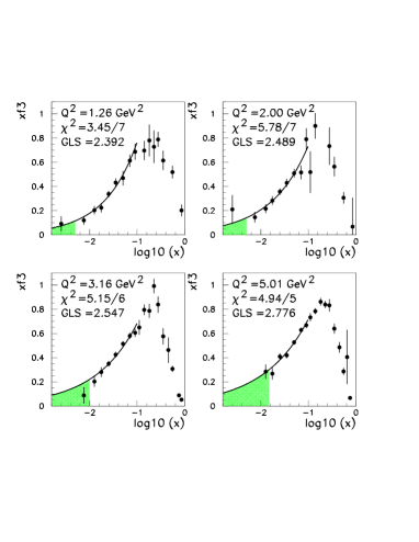
Figure 2: The structure function $F_{3}(x,Q^{2})$; GLS denotes the area under the curve. The shaded area is the contribution to GLS from the small $x$ extrapolation (from Ref.[34]).

The importance of the small $x$ extrapolation is highlighted in Fig. 2: it is clear that the choice of a specific functional form for the small $x$ extrapolation greatly constrains the result for the first moment, and can thus lead to an underestimate of the uncertainty due to the small $x$ extrapolation. The associated uncertainty has been studied in the polarized case in Ref.[10] by explicitly varying the functional form of the extrapolation. As a result, the value of $\alpha_{s}$ extracted from the Bjorken sum rule acquires a very large uncertainty $\Delta\alpha(M_{z})=\hbox{${\lower 1.0pt\hbox{$\scriptstyle+0.010$}}\atop{\raise 1.0pt\hbox{$\scriptstyle-0.024$}}$}$: the value includes statistical and extrapolation errors, but is dominated by the latter. This large error overwhelms any advantage which may be obtained from the accurate perturbative knowledge of the Wilson coefficient, and makes the extraction of $\alpha_{s}$ from it phenomenologically not viable with present data. In the unpolarized case a much more optimistic estimate ($\Delta\alpha(M_{z})=\hbox{${\lower 1.0pt\hbox{$\scriptstyle+0.006$}}\atop{\raise 1.0pt\hbox{$\scriptstyle-0.007$}}$}$) was obtained[34] by assuming a power-like behavior and varying the exponent of the power. In the unpolarized case, however, the issue is largely academic, since the need to use neutrino data to determine $F_{3}$ introduce several other sources of large systematic error, specifically related to the normalization of the cross section and the estimate of the charm contributions.

In conclusion, the extraction of $\alpha_{s}$ from DIS sum rules is theoretically very clean and could be a nice laboratory to study the convergence of the perturbative expansion of the leading twist Wilson coefficients and its relation to higher twist terms.[33] It is however not viable from a phenomenological point of view at present, mostly due to the insufficient kinematic coverage of the data which does not allow a reliable determination of the first moment of the structure functions.

2.3 Scaling violations at small $x$

Perhaps the most surprising experimental discovery at HERA is that the very strong scaling violations predicted by perturbative QCD at small $x$ are actually seen in the data, rather than being cut off by some nonperturbative mechanism: in the HERA kinematic range $F_{2}(x,Q^{2})$ rises at small $x$ in accordance with the QCD prediction,[35] rather than displaying the set-in of a nonperturbatively generated Regge-like behavior, which many expected and pre-HERA data seemed to suggest.[36] It is natural to think that if scaling violations are strong, then it must be possible to determine $\alpha_{s}$ accurately.

In fact, this turns out to be case also because of more subtle theoretical reasons. Indeed, the small $x$ rise of structure functions in perturbation theory is due to the fact that the gluon anomalous dimension has a pole in the $N$ plane at $N=1$. Solving the evolution equations it is easy to see that this pole translates into a rise of the gluon distribution and thus the structure function[35] $F_{2}\sim\alpha_{s}xg(x,Q^{2})\sim\alpha_{s}(Q^{2})\exp[2\gamma\sqrt{\xi\zeta}]$ (with $\xi=\ln{1\over x}$, $\zeta=\ln{1\over\alpha_{s}(Q^{2})}$ and $\gamma={12\beta_{0}}$), stronger than any power of $\ln{1\over x}$ but weaker than any power of $x$ (poles at smaller values of $\,\hbox{Re}\,N$ give contributions suppressed by powers of $x$ at small $x$).

Expanding the anomalous dimensions about the pole leads to a systematic expansion of the small $x$ structure function, where the $k$-th subleading order is suppressed by $\exp[\zeta/\xi]^{k/2}$.[37] The relevant point here is that truncating this expansion leads to an evolution equation (which is the small $x$ approximation to the Altarelli-Parisi equation) which is local in $x$ and $Q^{2}$; in particular, at leading order the gluon evolves according to a simple wave equation with a negative mass, while the (singlet) quark $q(x,Q^{2})$ is determined by the gluon:

$${\partial^{2}\left[xg(x,Q^{2})\right]\over\partial\xi\partial\zeta} = \gamma^{2}xg(x,Q^{2})$$ (4)

$${\partial\left[xq(x,Q^{2})\right]\over\partial\zeta} = {n_{f}\over 9}\gamma^{2}xg(x,Q^{2}).$$ (5)

Figure 3: Double scaling plot of the HERA data published up to 1996. The dashed line is the universal (parameter-free) prediction, computed with $\alpha_{s}(M_{z})=0.114$. (From Ref.[39]).

It follows that the leading asymptotic behavior of the structure function at small $x$ is a rise in the product of the two variables $\xi$ and $\zeta$. The scale of the rise is set by $\alpha_{s}(Q^{2})$ (through the definition of $\zeta$). The structure function depends only on the combination $\sigma\equiv\sqrt{\xi\zeta}$, and the asymptotic dependence on $\sigma$ is then universal (double asymptotic scaling[37]). It is important to notice that the asymptotic slope of this rise is a universal prediction: since asymptotically the running of $\alpha_{s}$ is driven by the leading order $\beta$ function and independent of the value of $\alpha_{s}$ (i.e. of $\Lambda$), the asymptotic slope of $F_{2}$ is a parameter-free prediction of QCD, and its experimental determination provides a basic test of the theory [11]. In fact, this is a more fundamental test of the QCD dynamics than those provided by the sum rules discussed in Sect. 2.2: the value of the slope of the small $x$ rise is fixed entirely by the Casimir operator of the gauge group and the number of quark flavors, whereas the values of the CCFR and Bjorken sum rule are determined, respectively, by the quark baryon number and by the nucleon $\beta$-decay constant.

However, for the sake of phenomenology it is again more convenient to assume the correctness of QCD evolution, and thus of this asymptotic prediction. In the region where the asymptotic prediction holds, but two-loop running effects are still relevant, it is then possible to extract $\alpha_{s}$ from the observed scaling violations. Such a determination appears to be particularly favorable, since these scaling violations are strong, and independent of the form of the parton distributions: in particular, one does not need an independent determination of the gluon distribution since the quark and gluon distribution are asymptotically proportional. There is however a major caveat, namely, whether one can trust NLO QCD evolution in the first place. This is not obvious, essentially because higher order corrections to the Altarelli-Parisi anomalous dimensions are expected to induce a yet stronger rise: the related problems will be discussed in Sect. 4. Also, one may think that eventually the perturbatively generated rise should be cut off by a nonperturbative mechanism.

A simple way of making sure that NLO evolution applies is to test for double asymptotic scaling (after dividing out universal subasymptotic corrections[38, 39]), to which it reduces at small $x$. Such a comparison is shown in Figure 3. Notice that the asymptotic prediction only depends on the value of $\alpha_{s}$: a description based on NLO evolution thus appears adequate.

Of course an accurate determination requires comparison to the full NLO prediction (rather than just the asymptotic behavior). Such a determination was done in Ref.[40, 41], on the basis of the data then available, with the result $\alpha_{s}(M_{z})=0.120\pm{0.005}({\rm exp.})\pm{0.009}({\rm th.})$. On top of the advantages already discussed (strong scaling violations, little dependence on the input parton distributions) it also turns out [41] that higher twist corrections are negligibly small in the HERA kinematic region (a result which recent data have confirmed[42]). The relatively large experimental error is due to the poor quality of the data then available, which also justified a crude treatment of the experimental systematics. The large theoretical error is mostly due to uncertainty related to the possibility of deviation from NLO evolution at small $x$, and to factorization and renormalization scale uncertainties: these could be both reduced if $\alpha_{s}$ were extracted from the current data (Fig. 1) which are much more precise and have a wider kinematic coverage.

Figure 4: Contribution to the $\chi^{2}$ of the fit from various datasets for the global fits of Ref.[43] (left) and Ref.[44] (right, adapted from the original ref.). In the latter case the curves, from top to bottom on the left denote the contributions from ZEUS, BCDMS, NMC, H1, SLAC, CCFR $F_{2}$, CCFR $F_{3}$ and E665.

The advantage of an extraction of $\alpha_{s}$ at small $x$ can be seen by comparing the contributions to the $\chi^{2}$ of a global fit of parton distributions to DIS data from various datasets as a function of $\alpha_{s}$ (Figure 4). Of course, a global fit doesn’t necessarily provide a good determination of $\alpha_{s}$ for each of the separate datasets because of the difficulty in combining the data from different experiments and in different kinematic region (and in particular their uncertainties). So, for instance, the BCDMS data, which give an excellent[18] determination of $\alpha_{s}$, would appear to have no minimum in the fit of Ref.[44]. Yet it is clear that the minimum in the small–$x$ data always is more stable, deeper, and self-consistent than any of the other datasets. A determination of $\alpha_{s}$ from the data shown in Fig. 1 is highly desirable and could be one of the most precise on the market.

3 Large $x$ and power corrections

Large values of $x$ correspond to the kinematical region where the invariant mass of the final state $W^{2}$ eq. (1) is small. In this region power corrections proportional to either $\Lambda^{2}\over W^{2}$ or $M^{2}\over W^{2}$ (where $M$ is the hadron target mass) are potentially large. Target mass corrections are of purely kinematical origin, and are thus completely understood from a theoretical viewpoint, and routinely included in current unpolarized data analyses. Note, however, that in the polarized case the computations necessary in order to implement the relevant phenomenology have been performed only recently.[45] Power corrections in $\Lambda^{2}\over W^{2}$ can be generated by the resummation of logs of $1-x$ which are present at all orders in perturbation theory.

3.1 Leading $\ln(1-x)$ and power corrections

Logs of $1-x$ are generated in the perturbative computation of the DIS cross section for kinematic reasons: as $x\to 1$ the phase space for the emission of an extra parton is suppressed, so that each extra emissions carries a factor of $\alpha_{s}(Q^{2})\ln(1-x)$. At the leading logarithmic level, these contributions are resummed[46] by replacing

$$\alpha_{s}(Q^{2})\to\alpha_{s}((1-x)Q^{2})={\alpha_{s}(Q^{2})\over 1+\beta_{0}\alpha_{s}(Q^{2})\ln(1-x)}$$ (6)

and bringing the coupling inside the $x$ integration when evaluating the Mellin moments of the splitting function on the r.h.s of the evolution equations eq. (3). This means that the coupling is effectively evaluated at the scale $W^{2}$ eq. (1); as $x\to 1$, $W^{2}\to 1$ and the growth of the coupling in the infrared generates a factorial divergence in the perturbative expansion, which is in turn related to a powerlike correction to the structure function.

This can be understood by considering the, say, first Mellin moment of $\alpha_{s}$ after the substitution eq. (6):

$$I[\alpha_{s}]\equiv\int_{0}^{1}\!dx\alpha_{s}((1-x)Q^{2}) = \alpha_{s}(Q^{2})\sum_{k=0}^{\infty}(-1)^{k}[\beta_{0}\alpha_{s}(Q^{2})]^{k}\int_{0}^{1}\!dx\,\ln(1-x)^{k}$$ (7)

$$= \alpha_{s}(Q^{2})\sum_{k=0}^{\infty}k!(\alpha_{s}(Q^{2})\beta_{0})^{k}.$$

The factorially divergent series can be summed by Borel resummation, i.e. by defining

$$I[\alpha_{s}]\equiv\int_{0}^{\infty}\!ds\,e^{-s/\alpha_{s}(Q^{2})}B[s].$$ (8)

It is easy to see that $B[s]={1\over 1-s\beta_{0}}$. Thus, if we want to determine $I[\alpha_{s}]$ from eq. (8) we must integrate over the pole at $s=s_{0}\equiv{1\over\beta_{0}}$. This generates a contribution to $I[\alpha_{s}]$ proportional to $e^{-s_{0}/\alpha_{s}(Q^{2})}={\Lambda^{2}\over Q^{2}}$. Reconstructing the full $x$ dependence from the computation of all Mellin moments shows that the power suppressed contribution is actually proportional to $\Lambda^{2}\over W^{2}$, i.e. rapidly growing at small $x$.

The strength of this $\Lambda^{2}\over Q^{2}$ contribution is ambiguous however: for instance, its sign depends on whether the path of integration along $s$ is taken above or below the pole. The ambiguity is to be expected since we have obtained the result from a leading twist computation, i.e. not including terms suppressed by powers of $Q^{2}$, and can only be fixed by performing the computation to power accuracy. Of course, as long as we are interested in the leading twist, leading $\ln(1-x)$ result, we may simply refrain from expanding out $\alpha_{s}((1-x)Q^{2})$.

This suggests two directions of progress in the description of the large $x$ region. On the one hand, we may push the resummation of $\ln(1-x)$ contributions beyond the leading log level. Indeed, the next-to-leading resummation is also known;[47] and a systematic method to resum subleading contributions to all orders has been suggested recently.[48] This determines the large $N$ behavior of the anomalous dimensions and coefficient functions. On the other hand, we may use the fact that the all-order summation of leading twist contributions generates power-suppressed terms as a means to acquire information on the higher twist terms in the operator-product expansion. Considerable progress has been made recently in the latter direction by means of the so–called renormalon method.

3.2 Renormalons and phenomenology

Because the structure function is a physical observable, the ambiguity proportional to $\Lambda^{2}\over Q^{2}$ generated by the Borel resummation of classes of leading twist contributions must be cancelled by an equal and opposite ambiguity in the next-to-leading twist contribution. Indeed, such an ambiguity arises when regulating the power ultraviolet divergence of the next-to-leading twist, i.e., the pole in the Borel transform must cancel between leading and next-to-leading twist. We can then take the coefficient of the pole in the leading twist as an estimate of the full next-to-leading twist computation. The rationale for this is the same as when estimating a NNLO corrections by varying the factorization scale in a NLO computation. Of course, we would expect this estimate to be only qualitatively correct.

A specific class of factorially divergent contribution, related to the small momentum region of integration on loop momenta (infrared renormalons) can be isolated and computed for a variety of observables, and may be used to this purpose.[49] In the case of DIS, the renormalon contributions to the coefficient functions which relate structure functions to parton distributions have been computed both in the nonsinglet[50] and singlet[51] sector (the contributions to the nonsinglet splitting functions are also known[52], but have not been used for phenomenology). One can then convolute this $\Lambda^{2}\over Q^{2}$ contribution to the coefficient function with parton distributions taken from a NLO, leading twist fit of structure functions data, and view the result as an estimate of the $O\left({\Lambda^{2}\over Q^{2}}\right)$ part of the structure function itself, up to an unknown coefficient. The result can be compared to available phenomenological fits,[18] where the structure function is parameterized as

$$F_{2}(x,Q^{2})=F_{2}^{\rm l.t}(x,Q^{2})+{h(x)\over Q^{2}},$$ (9)

and the function $h(x)$ is treated as a free parameter for each $x$ data bin.

After adjusting the coefficient (to about three times of what would be obtained by Borel transform integrating below the pole, as discussed in Sect. 3.1) the agreement with the data appears to be excellent: in particular, the shape (as a function of $x$) of the observed twist four (i.e. $O\left({1\over Q^{2}}\right)$) contribution to $F_{2}$ appears to agree very well with the renormalon estimate. This poses a problem, since quantitative agreement is found, whereas only a qualitatively correct description was expected. The result is especially surprising in view of the fact that higher twist contributions correspond to operators which measure multiparton correlations in the target and should thus be target-dependent, whereas the $O\left({1\over Q^{2}}\right)$ contribution computed from renormalons is universal, since it comes from a coefficient function.

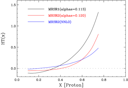
Figure 5: Higher twist contribution eq. (9) to $F_{2}$ from the fit of ref.[53]. The curves are labelled from top to bottom on the right.

A hint on the possible origin of this state of affairs comes from a recent phenomenological analysis[53] of the BCDMS[3], SLAC[5] and CCFR[20] $F_{2}$ data (see Fig.5). The fitted higher twist contribution agrees well with previous fits,[18] even though here a different[54] set of parton distributions and a wider dataset are used. However, if the value of $\alpha_{s}$ used in the computation of the leading twist part is changed from the low value used in Ref.[18] to a larger value, a substantial reduction of the higher twist contribution is observed. If $F_{2}$ is computed by folding the NLO partons with the NNLO coefficient function[55] the higher twist is further reduced. A decrease of the fitted higher twist contribution as more perturbative orders are included has also been found in an analysis of the CCFR $F_{3}$ data;[24] while the strong anticorrelation between the value of $\alpha_{s}$ and the size of the higher twist contributions has been observed in a recent reanalysis of the BCDMS/SLAC data[26] and in a phenomenological extraction of higher twists from “world” data.[56]

This means that the fit doesn’t really distinguish between log and power behavior: the higher twist correction extracted from the fits is in large part a parameterization of missing leading twist contributions, because of the truncation to NLO, or because the value of $\alpha_{s}$ is too small. This explains naturally the success of the renormalon calculation, which is equal to the resummation of higher order contributions, and thus provides a good approximation to such missing higher order terms. Notice that the leading $\ln(1-x)$ terms discussed in Sect. 3.1 are included in the renormalon estimate. But this also means that the “dynamical” (i.e. target-dependent) part of the higher twist, which is unrelated to higher perturbative orders and would spoil this agreement, must be subdominant (i.e. the higher twist is “ultraviolet dominated”[57]). In principle, it is alternatively possible that dynamical higher twists have a similar functional form as the renormalon higher twist, and are thus not easily disentangled from them. This is presumably true in the $x\to 1$ limit, in that a $1\over 1-x$ behavior is expected to be generic on kinematic grounds, and it indeed happens if dynamical higher twists are e.g. estimated in a simple model based on free-field theory.[58] It seems rather unlikely in general though, and it appears more natural to simply conclude that dynamical higher twists are smaller, and hidden by the renormalon contribution.

All this has also interesting implications for the leading twist phenomenology: it implies that the value of $\alpha_{s}$ extracted from log scaling violations can be underestimated if higher twists are large in the fit and, more importantly, the error on $\alpha_{s}$ can be underestimated if higher twists are not allowed to vary enough. These problems should be mitigated in a determination of $\alpha_{s}$ at small $x$, where $W^{2}$ is large and indeed higher twists appear to be small.[40, 42]

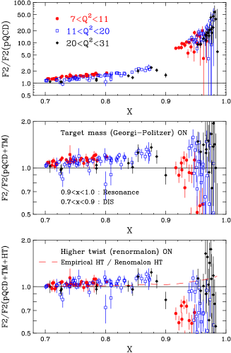
Figure 6: Comparison of the $F_{2}$ data with the NLO calculation based on the partons of Ref.[54], without power corrections (upper), with target mass corrections (middle), with target mass and renormalon corrections (from ref.[53]). “Empirical HT” refers to a model functional form for $h(x)$ eq. (9).

One is thus led to conclude that there is a hierarchy in power corrections to structure functions at large $x$ (Fig.6): target mass corrections are characterized by a relatively large scale of order of the target mass $M\sim 1$ GeV; higher twists due to the resummation of higher orders in the $\overline{\rm MS}$ scheme have a characteristic scale of several hundreds of MeV; and “dynamical” higher twist corrections appear at a yet smaller scale. Even though there is no understanding of this subdominance, it is not necessarily problematic: one would expect the natural scale of dynamical higher twists to be of order $\Lambda$, and current data are compatible with this. If however the scale turned be much smaller, this would pose an interesting dynamical problem: naive perturbation theory would appear to work at low $Q^{2}$ better than it ought to. Be that as it may, the phenomenological extraction[59] of the dynamical higher twist corrections, which would give access to parton correlations in the nucleon, appears to be a very difficult challenge which will require new experimental information.

4 Structure functions at small $x$

As we discussed in Sect. 2.3, the rise of $F_{2}(x,Q^{2})$ at small $x$ observed at HERA is in spectacular agreement with the prediction obtained by approximating the NLO anomalous dimensions with their highest rightmost singularities in $N$-space (leading singularities, henceforth). This immediately raises a problem: higher order (in $\alpha_{s}$) contributions to thr anomalous dimensions contain higher order poles, associated to higher order powers of $\ln{1\over x}$. One has thus to face the problem of summing these contributions. Because at small $x$ according to eq. (1) $W^{2}\approx{Q^{2}\over x}$, this is related to the determination of the leading high energy behavior of parton-parton scattering cross sections.

4.1 Altarelli-Parisi equations and summation of $\ln{1\over x}$

While solving the Altarelli-Parisi sums leading logs of $Q^{2}$, the inclusion of suitable higher order terms in the anomalous dimension allows one to also sum other logs: for instance we discussed in sect. 3.1 how to sum leading logs of $1-x$. The leading singularities of the anomalous dimensions in the gluon sector have the generic form[60]

$$\gamma^{ij}=\sum_{k=0}^{\infty}\alpha_{s}^{k}\gamma^{(k)\,ij}$$ (10)

$$\gamma^{(k)\,ij}=\sum_{n=1}^{\infty}a_{n}^{(k)\,ij}\left(C{\alpha_{s}\over N-1}\right)^{n}$$ (11)

where $C={12\log 2\over\pi}$ and the coefficients satisfy $\lim_{n\to\infty}{a^{ij}_{n+1}\over a_{n}^{ij}}=1$. At leading order in $\alpha_{s}$, the only nonvanishing coefficients are in the gluon sector, where they satisfy $a_{n}^{(0)\,gq}={4\over 9}a_{n}^{(0)\,gg}$ (with $n\geq 1$), and can be extracted[60] from knowledge of the leading log high energy behavior of QCD perturbative cross sections, which is in turn found by solution of the BFKL equation.[61] If such contributions are included in the anomalous dimensions, the solution to the Altarelli–Parisi equation contains all leading logs of $1\over x$, because a $k$-th order pole in $N$ space corresponds to a $\ln{1\over x}^{k}$ contribution.

Naively, one may think that since the series in eq. (11) has unit radius of convergence, one must resum all orders in $\ln{1\over x}$ whenever the expansion parameter $\Xi(x,Q^{2})\equiv C\alpha(Q^{2})\ln{1\over x}\sim 1$. This is problematic because $C$ is very large so $\Xi(x,Q^{2})\gg 1$ in the HERA region, and in fact $\Xi(x,Q^{2})>1$ also in most of the SLAC and all of the NMC region (see Fig. 7): the small $x$ region is outside the radius of convergence of the series. This, in the pre-HERA age, led to the conclusion that the perturbative expansion eq. (11) breaks down at small $x$.[62]

This conclusion is however unwarranted, because the quantity of direct physical interest is the Altarelli-Parisi splitting function, related by inverse Mellin transformation to the anomalous dimension eq. (10-11). Now, the inverse Mellin transform is essentially the same as the Borel transform discussed in Sect. 3.1, so if the anomalous dimension as a series in $\alpha_{s}$ eq. (11) has a finite radius of convergence, the splitting function has an infinite radius of convergence for all finite $x$. It follows that the leading $\ln{1\over x}$ summation converges for all $x$, and can thus be used down to arbitrarily small $x$: in each $(x,Q^{2})$ region, it is sufficient to sum the first $k$ terms in eq. (11), where $[\Xi(x,Q^{2})]^{k}/k!\sim 1$, i.e. (from Stirling formula) $k\approx 2.7\Xi$ for $\Xi\mathrel{\mathchoice{\lower 0.86108pt\vbox{\halign{$\m@th\displaystyle\hfil#$\cr>\crcr\sim\crcr}}}{\lower 0.86108pt\vbox{\halign{$\m@th\textstyle\hfil#$\cr>\crcr\sim\crcr}}}{\lower 0.86108pt\vbox{\halign{$\m@th\scriptstyle\hfil#$\cr>\crcr\sim\crcr}}}{\lower 0.86108pt\vbox{\halign{$\m@th\scriptscriptstyle\hfil#$\cr>\crcr\sim\crcr}}}}1$. Notice the difference in comparison to the large $x$ case, discussed in Sect. 3.1, where the leading large $N$ anomalous dimension diverges factorially, so the leading $\ln(1-x)$ series has a finite radius of convergence (cfr. eq. (6)), one must resum an infinite number of terms, and the resummation breaks down when $x\to 1$.

In fact, it can be shown[63] that the Altarelli-Parisi equation with leading-singularity anomalous dimensions $\gamma^{(0),\,ij}$ eq. (10) is completely equivalent, up to higher twists, to the BFKL equation (in the inclusive case), which describes the leading log high energy asymptotics. It follows that one may proceed in two equivalent ways: either one determines the LO coefficients $a^{(0)\,ij}$ eq. (11) from the BFKL kernel, and then one inverse-Mellin transforms the series eq. (11) term by term, thereby obtaining a convergent series which may be truncated at finite order.[64] Or, alternatively, one constructs “nonperturbatively”, i.e. numerically the leading-singularity anomalous dimension as a function of $a/N$ directly from the BFKL kernel. [65]

Either way, one is lead to a perturbative expansion of the small-$x$ splitting function

$$P^{ij}(x,Q^{2})=P^{(0)\,ij}+\alpha_{s}P^{(1)\,ij}+\dots$$

$$P^{(p)\,ij}(x,Q^{2})={1\over x}\sum_{n=0}^{\infty}a_{n+1}^{(p)\,ij}\left(C{\alpha_{s}\ln{1\over x}\over n!}\right)^{n}.$$ (12)

In the quark sector, the coefficients $a^{qj}_{n}$ start at $O(\alpha_{s})$ and are thus subleading compared to the gluon ones; they are however also known.[66] It is thus possible to determine the splitting functions $P^{ij}$ to leading nontrivial order, add them on top of usual NLO splitting function (with suitable matching conditions), and compare the result to the HERA data[64, 65].

Figure 7: (Left) Contours of constant $\Xi\equiv C\alpha_{s}(Q^{2})\ln({1\over x})=1,2\dots 20$ (from bottom to top) in the $(x,Q^{2})$ plane. as a function of $x$ and $Q^{2}$.  (Right) The ratio of NLO to LO splitting functions eq. (11) in various factorization schemes: $\overline{\rm MS}$(solid), $Q_{0}$[73] (dotted), “physical”[68] (dashed and dot-dashed) (from Ref.[72]).

Unfortunately, the results of this comparison are discouraging: as long as the HERA data were still relatively scarce, no evidence of the $\log{1\over x}$ summation could be seen,[64] but as soon as they became accurate enough, the presence of such effects could be excluded to very high accuracy, essentially because they induce much stronger scaling violations than observed in the data.[67] In fact, the only way current data can be reconciled with evolution equations that include a summation of small $x$ effects is by artificially fine–tuning the factorization scheme in such a way as to remove these effects from the measured region.

A possible way out of this impasse consists of exploiting the wider factorization scheme freedom which is related to the summation of small-$x$ contributions: for instance, one can always reabsorb any undesirable scaling violations induced by the leading-order contributions in eq. (10), which only appear in the gluon sector, in a redefinition of the gluon normalization, at the only cost of changing the next-to-leading coefficients $a^{(1)\,gg}_{n}$. It could then be that the effects which cause disagreement with the data are a spurious consequence of the choice of factorization scheme, and would disappear in a “physical” scheme where each parton distribution is identified with a physical observable.[68] In order to check whether this is the case, however, the full set of NLO coefficients $a_{n}^{ij}$ eq. (11) is needed: one may then verify whether in this scheme the undesirable scaling violations actually disappear.

Thanks to the recent calculation of the next-to-leading corrections to the high–energy QCD asymptotics,[69] which allows a determination of the next-to-leading coefficients $a_{n}^{(1)\,gg}$, it is now possible to resolve this issue. The outcome of the calculation, however, brought a new surprise: the NLO coefficients are negative and grow very large[70, 71] in comparison to the leading order ones as the order $k$ in eq. (12) grows. In fact, it can be shown both numerically[70] and analytically[72] that the ratio of the NL contribution to the splitting function to the leading order grows linearly as a function of $\Xi$, and in fact overwhelms the leading order for any reasonable value of $x$ and $Q^{2}$ (fig. 7). The problem is in fact worse in “physical” schemes where the ratio grows as $\Xi^{3/2}$; the same happens in the so-called $Q_{0}$ scheme[73] (designed to reduce perturbative corrections in the quark sector), as well as in the momentum conserving scheme[74], though the slope of the growth is somewhat smaller in the latter case.

The growth of the NLO “correction” with respect to the leading order means that the NLO $P^{(1)}$ eq. (12), though formally subleading, is actually enhanced at large $\Xi$ with respect to $P^{(0)}$: even though it is suppressed by an extra power of $\alpha_{s}$, at sufficiently small $x$ it always takes over due to the growth of $\Xi$ with $\ln{1\over x}$ at fixed $\alpha_{s}$. Hence, it is the perturbative expansion of the leading $\ln{1\over x}$ contributions to the Altarelli-Parisi equations defined by eq. (12) which breaks down.

On the one hand, this is good news, in that it explains why the inclusion of the leading $\ln{1\over x}$ summation $P^{(0)\,ij}$ spoils the agreement with the data: these terms are actually not leading in the HERA region, and thus there is no reason why including them while not including more important contributions should improve the phenomenology. On the other hand, however, the fact that standard NLO works at all — not only at HERA, but also in the SLAC or NMC region (see Fig. 7) — is now puzzling: there must be very large cancellations in the anomalous dimension eq. (11), or, otherwise stated, the expansion eq. (12) is pathological.

It is thus necessary to reorganize the expansion. Now, it can be shown[72] that the rise of the NL correction is entirely generic — it could have been predicted without waiting the outcome of the Fadin-Lipatov calculation: the ratio of the N^kLO to the LO splitting functions eq. (12) behaves as ${P^{(k)}\over P^{(0)}}\sim[\alpha_{s}\ln({1\over x})]^{2k-1}$. This behavior is related to the fact that generically the anomalous dimensions $\gamma^{(k)}$ eq. (11) has a (2k-1)—th order pole at ${C\alpha_{s}\over N}=1$. The slope of the $k$-th order rise is determined by the residue of the corresponding pole, which can in turn be simply expressed in terms of the $k$–th order corrections to high-energy asymptotics.

It is possible to eliminate this singularity in the anomalous dimension, and thus the instability of the perturbative expansion, by suitably choosing the factorization scale order by order in $\alpha_{s}$. This is however a fine-tuning: even small variations of the factorization scale around the optimal scale bring back immediately the instability (see Fig. 8) A better option consists of reabsorbing into the leading order $P^{(0)}$ all contributions which lead to the small $x$ growth of the formally subleading $P^{(i)}$. It turns out that this can be done in a completely unambiguous way by subtracting terms related to the residues of the poles in the anomalous dimensions.

Figure 8: The ratio of NLO to LO splitting functions eq. (11) in the DIS scheme after resummation (solid), with fine-tuned scale (dashed) and scales a factor of two either side of the fine-tuned one (dotted). (from Ref.[72])

The overall ambiguity introduced by the procedure is contained in a single parameter $\lambda$, which could only be determined by resumming the splitting function to all orders. This parameter governs the all-order asymptotic behavior of the splitting function $P(x,Q^{2})$ eq. (12): $P(x,Q^{2})\sim(\ln{1\over x})^{3/2}x^{\lambda}$. The ensuing splitting functions can be viewed as a resummation of the original series: the leading order resummed $P^{(0)}$ depends on the all-order resummed parameter $\lambda$, but the ratios of all higher order $P^{(i)}$ to $P^{(0)}$ is fixed, and tend asymptotically to a constant as $x\to 0$ (Fig. 8).

In an Altarelli-Parisi framework this does not entail loss of predictivity, since the $Q^{2}$-independent part of the $x$ dependence of the structure function cannot be determined anyway. However, it does show that even assuming that the asymptotic small $x$ behavior of structure functions is determined by perturbative QCD asymptotics, it cannot be determined in any finite order computation and would require an all-order resummation of the small-$x$ expansion.

4.2 Energy evolution

The resummation of the the leading $\ln{1\over x}$ contributions to structure functions discussed in the previous section is not the end of the story, however. So far, we have discussed leading $\ln{1\over x}$ contributions which are generated when solving evolution equations in $Q^{2}$, i.e. the Altarelli-Parisi equations. This, however, is an indirect manifestation of a more fundamental phenomenon, namely, the fact that the high-energy behavior of the gluon-gluon scattering cross section in perturbative QCD is dominated by energy logs.

In DIS energy logs appear as $\ln W^{2}\sim\ln{1\over x}$, and can be summed by means of an equation for evolution in $1\over x$. This is accomplished by the BFKL equation,[61] which in the fully inclusive case can be written in the same form as the usual QCD evolution equation, but with the roles of the two kinematic variables $x$ and $Q^{2}$ interchanged. To this purpose, it is necessary to take a Mellin transform with respect to $Q^{2}$ and define kernels $\chi(M)$ as functions of the associate variable $M$, which can then be used to evolve in $\xi\equiv\ln{1\over x}$:

$${d\over d\xi}G(x,M)=\alpha_{s}\chi(M)G(x,M)$$

$$\quad G(x,M)\equiv\int_{0}^{\infty}{dQ^{2}\over Q^{2}}\left({Q^{2}\over\Lambda^{2}}\right)^{-M}G(x,Q^{2})$$ (13)

$$\quad\chi(M)=\chi^{(0)}(M)+\alpha_{s}\chi^{(1)}+\dots,$$

where $G(x,Q^{2})$ is the leading eigenvector of the anomalous dimension matrix eq. (10) (i.e. the one associated to the only nonvanishing leading–order eigenvalue), which at leading order is just $G(x,Q^{2})=xg(x,Q^{2})$ with $g(x,Q^{2})$ the gluon distribution. Since $G(x,Q^{2})$ behaves as a constant at large $Q^{2}$ (Bjorken scaling) and falls linearly as $Q^{2}\to 0$ (for kinematic reasons[1]), the (leading twist) physical region in $M$ space is $0<M<1$. At leading order, $\chi^{(0)}(M)=2\gamma-\psi(M)-\psi(1-M)$ (where $\psi(M)$ is the digamma function) — the celebrated BFKL kernel — and the recent FL calculation[69] in the inclusive case amounts to a determination of the next-to-leading correction $\chi^{(1)}(M)$.

Figure 9: The kernel $\chi(M)$ eq. (4.2) plotted as a function of $M$. The curves from top to bottom in the middle are the LO result with $\alpha_{s}=0.1$ and the NLO result with $\alpha_{s}=0.1$, 0.05, 0.03, 0.01, 0.005. (adapted from Ref.[70])

The qualitative behavior of the kernel is changed dramatically by the NL correction (see Fig. 9). To understand the effect of this change, solve the evolution equation eq. (4.2) and construct $G(x,Q^{2})$ by inverting the Mellin transform:

$$G(x,Q^{2})=\int_{-i\infty}^{i\infty}\!{dM\over 2\pi i}\,\left({Q^{2}\over\Lambda^{2}}\right)^{M}e^{\xi\chi(M)}G_{0}(M).$$ (14)

The asymptotic behavior of the integral at small $x$, i.e. large $\xi$ is determined by saddle point. Since the integration path runs along the imaginary axis, the saddle is a minimum of $\chi(M)$ along the real axis, which at leading order is located at $M={1\over 2}$, where $\chi^{(0)}(1/2)=4\ln 2$. But at NLO there is no real minimum, and the real saddle is thus replaced by two complex saddles (which must occur in complex conjugate pairs by definition of the kernel as the Mellin transform of a real splitting function).[70, 75] Hence the NLO, rather than being a small correction to the LO, changes the asymptotic behavior, and in fact leads to an oscillatory, unphysical behavior at large $\xi$. In particular, the value of $\chi(1/2)$ has no special meaning if $\chi$ is computed at NLO. Of course, at small enough $\alpha_{s}$ i.e. high enough scales, the leading order behavior is recovered: however, this only happens (Fig. 9) at values of $\alpha_{s}\mathrel{\mathchoice{\lower 0.86108pt\vbox{\halign{$\m@th\displaystyle\hfil#$\cr<\crcr\sim\crcr}}}{\lower 0.86108pt\vbox{\halign{$\m@th\textstyle\hfil#$\cr<\crcr\sim\crcr}}}{\lower 0.86108pt\vbox{\halign{$\m@th\scriptstyle\hfil#$\cr<\crcr\sim\crcr}}}{\lower 0.86108pt\vbox{\halign{$\m@th\scriptscriptstyle\hfil#$\cr<\crcr\sim\crcr}}}}0.01$ which correspond to a scale above the Planck mass.[70]

The original calculation on which these results are based,[69] which is the result of an effort of years, has been in large part checked independently: most of the individual real and virtual amplitudes have been recomputed with different techniques;[76] and the elaborate computation that takes from the individual amplitudes to the kernel has also been checked.[77] It thus appears unlikely that the result[69] is erroneous. The saddle point estimate of the asymptotic behavior has also been checked by more accurate calculations, which have confirmed the unphysical oscillatory behavior of the cross–section.[78, 79]

The problem posed by this unphysical behavior is separate from that discussed in Sect. 4.1. Indeed, there we saw that the naive small $x$ expansion of the anomalous dimension must be reorganized in such a way that the terms which contribute to the asymptotic small $x$ behavior to all orders in the expansion eq. (10) are resummed into a parameter $\lambda$, and included into the leading order of a resummed expansion. Now, we are studying how the all-order asymptotic behavior can be derived from $\chi$, and we see that if $\chi$ is computed to NL order, the associate asymptotic behavior is unphysical. It therefore looks like a further resummation of $\chi$ is required.

Several partial resummations of formally subleading corrections to $\chi$ have thus been suggested. First, one can attempt to resum logs of $Q^{2}$ related to the running of the coupling[80], though this actually seems to make things worse.[79] Also, one may try to optimize the scale choice by the BLM method[81]: this goes in the right direction, but does not completely remove the instability. A further option consists of noting that the definition of the leading energy logs which are being resummed requires a choice of scale: for instance, in DIS at small $x$, $s=W^{2}\approx{Q^{2}\over x}$, and the resummation of $\ln{1\over x}$ may be more generally viewed as a resummation of $\ln{s\over s_{0}}$ with $s_{0}=Q^{2}$. Different choices of $s_{0}$ then lead to different subleading corrections, and a resummation of these “scale-dependent” corrections may change the properties of the evolution equation eq. (4.2).[82] A specific resummation of such corrections has been advocated on the grounds that it removes some undesirable singularities of $\chi(M)$ at $M=0$, thus leading to an improved asymptotic behavior[82, 83]. This does not, however, lead to an unambiguous prescription. Use of an evolution equation based on angular ordering seems to further increase the theoretical ambiguities.[84]

A perhaps more fundamental possibility [85, 86] is to re-examine the assumptions on the high-energy asymptotics that go into the NL determination of $\chi$. In particular, by introducing physically motivated kinematic cuts in the course of the determination of $\chi(M)$ one can reshuffle contributions between the NL $\chi^{(1)}$ and the LO kernel $\chi^{(0)}$ while only changing the (unknown) NNL terms. Again, the shortcoming of the approach is that it introduces an ambiguity, in the form of a dependence on a “cutoff” parameter. However, the ensuing NL result is then well-behaved in a reasonable range of values of this cutoff. The ambiguities can be somewhat reduced[87] by again resumming “scale dependent” corrections along the lines of Ref.[82]

In conclusion, the ambiguities encountered when trying to construct an energy evolution equation appear to be related to the choice of the appropriate large scale. Indeed, on the one hand the large log which is treated as leading and summed by the evolution equations is $\xi$, associate to the large scale $W^{2}$, but on the other hand the hard scale which guarantees the validity of perturbative factorization and the smallness of $\alpha_{s}$ is $Q^{2}$. The need to reconcile these two large scales appears to be at the origin of the difficulties of perturbation theory at small $x$. A radical suggestion, based on the idea that $W^{2}$ should also be used as a factorization scale, was discussed in ref.[63]; a proof of the corresponding factorization theorems would however be required in order for this approach to be viable beyond leading order. We must conclude that no reliable theory of small $x$ evolution is yet available. The success of simple NLO perturbation theory and the small $x$ approximation to it still lacks a completely fully satisfactory explanation.

5 The embarrassing success of QCD

The application of perturbative QCD to inclusive deep-inelastic scattering is embarrassingly successful. In many ways, QCD is enjoying the same sort of success as the electroweak sector of the standard model. Whether the lack of evidence for nonstandard effects should be considered a triumph or a disappointment is of course matter of opinion. However, in many instance things are now too easy: we do not see deviations from the simple leading log behavior even in kinematic regions where we might have expected them, in particular at very large and very small $x$. This reveals that our understanding of perturbative QCD and its limitations is still not satisfactory from a theoretical viewpoint.

References

- [1] R.K. Ellis, W.J. Stirling and B. Webber, QCD and Collider Physics (Cambridge U.P., Cambridge, U.K., 1996); R. G. Roberts, The structure of the proton (Cambridge U.P., Cambridge, U.K., 1990)
- [2] G. Altarelli, Phys. Rep. 81, 1 (1982)
- [3] BCDMS Coll., A. Benvenuti et al., Phys. Lett. B223, 485 (1989)
- [4] NMC Coll., M. Arneodo et al., Phys. Lett. B364, 107 (1995)
- [5] L. W. Whitlow et al., Phys. Lett. B282, 475 (1992)
- [6] H1 Coll., presented by A. De Roeck at “Nucleon ’99”, Frascati, June 1999.
- [7] See e.g. SMC Coll., B. Adeva et al., Phys. Rev. D58, 112001 (1998); T. Çuhadar, Ph. D. Thesis, Amsterdam Free University, 1998
- [8] M. Rueter, hep-ph 9807448; A. Donnachie and P. V. Landshoff, Phys.Lett. B437, 408 (1998); P. Desgrolard, A. Lengyel and E. Martynov, hep-ph/9811380
- [9] W. Buchmüller and D. Haidt, hep-ph/9605428; D. Haidt, talk at the DIS99 meeting
- [10] G. Altarelli et al., Nucl. Phys. B496, 337 (1997); Acta Phys. Pol. B29 1145 (1998)
- [11] R. D. Ball and S. Forte, Phys. Lett. B336, 77 (1994)
- [12] For reviews see E. Predazzi, hep-ph/9809454; A. Hebecker, hep-ph/9905226; W. Buchmüller, hep-ph/9906550
- [13] L. Trentadue and G. Veneziano, Phys. Lett. B323, 201 (1993)
- [14] D. De Florian and R. Sassot, hep-ph/9808300
- [15] Particle Data Group, C. Caso et al., Eur. Phys. J. C3, 1 (1998)
- [16] Particle Data Group, R. M. Barnett et al, Phys. Rev. D54, 1 (1996)
- [17] H1 Coll., T. Ahmed et al, Phys. Lett. B346, 415 (1995); ZEUS Coll., M. Derrick et al, Phys. Lett., B363, 201 (1995); H1 Coll., subm. to ICHEP98 (Vancouver, July 1998), Abstract 528
- [18] M. Virchaux and A. Milsztajn, Phys. Lett. B274, 221 (1992)
- [19] NMC Coll., M. Arneodo et al., Phys. Lett. B309 222 (1993)
- [20] CCFR Coll., W. G. Seligman et al., Phys. Rev. Lett. 79, 1213 (1997)
- [21] CCFR Coll., P. Z. Quintas et al., Phys. Rev. Lett. 71, 1307 (1993).
- [22] S. A. Larin, T. van Ritbergen and J. A. M. Vermaseren, Nucl. Phys. B427, 41 (1994); Nucl.Phys. B492, 338 (1997)
- [23] A. L. Kataev et al., Phys. Lett B417, 374 (1998)
- [24] A. L. Kataev, G. Parente and A. V. Sidorov , hep-ph/9905310.
- [25] J. Santiago and F. J. Yndurain, hep-ph/9904344
- [26] S. Alekhin, Phys.Rev. D59, 114016 (1999)
- [27] S. I. Alekhin and A. L. Kataev Phys. Lett. B452 402 (1999)
- [28] See e.g. S. Forte, hep-ph/9610238; R. D. Ball, hep-ph/9812383
- [29] A. De Roeck et al., Eur. Phys. J. C6,121 (1999)
- [30] J. Huston et al., Phys. Rev. D58, 114034 (1998)
- [31] R. D. Ball, S. Forte and G. Ridolfi, Phys. Lett. B378, 255 (1996)
- [32] S. A. Larin and J. A. M. Vermaseren, Phys. Lett. B259, 345 (1991)
- [33] J. Ellis et al., Phys. Lett. B366, 268 (1996)
- [34] CCFR Coll., J. H. Kim, D. A. Harris et al., Phys. Rev. Lett. 81, 3595 (1998)
- [35] A. de Rùjula et al., Phys. Rev. D10, 1649 (1974)
- [36] NMC Coll., M. Arneodo, Phys. Lett. B295, 159 (1992)
- [37] R. D. Ball and S. Forte, Phys. Lett. B335, 77 (1994)
- [38] R. D. Ball and S. Forte, Acta Phys. Pol. 26, 2079 (1995)
- [39] L. Mankiewicz, A. Saalfeld and T. Weigl, Phys. Lett. B393, 175 (1997)
- [40] R. D. Ball and S. Forte, Phys. Lett. B358, 365 (1995)
- [41] R. D. Ball and S. Forte, hep-ph/9607289
- [42] A. Martin et al., hep-ph/9808371
- [43] CTEQ Coll., H. L. Lai et al., Phys. Rev. D55, 1280 (1997),; W. K. Tung, hep-ph/9608293
- [44] A. Martin et al., Eur. Phys. J. C4, 463 (1998)
- [45] A. Piccione and G. Ridolfi, Nucl. Phys. B513, 301 (1998)
- [46] D. Amati et al., Nucl. Phys. B173, 329 (1980)
- [47] S. Catani and L. Trentadue, Nucl. Phys. B327, 323 (1989); G. Sterman, Phys. Lett. B179, 281 (1986)
- [48] R. Akhoury, M. G. Sotiropoulos and G. Sterman, Phys. Rev. Lett., 81, 3819 (1998)
- [49] M. Beneke, hep-ph/9807443 and ref. therein
- [50] E. Stein et al, Phys. Lett. B376, 177 (1996); M. Dasgupta and B. R. Webber, B382, 273 (1996); M. Meyer-Herrmann et al., Phys. Lett. B383, 463 (1996)
- [51] E. Stein et al., hep-ph/9803342
- [52] U. Aglietti, Nucl. Phys. B451, 605 (1995)
- [53] U. K. Yang and A. Bodek, hep-ph/9809480; U. K. Yang, talk at ICHEP98 (Vancouver, July 1998), unpublished
- [54] A. D. Martin, R. G. Roberts and J. Stirling, Phys. Lett. B387, 419 (1996)
- [55] E. B. Zijlstra and W. L. van Neerven, Nucl.Phys. B383, 525 (1992)
- [56] S. Liuti, hep-ph/9809248
- [57] M. Beneke, V. M. Braun and L. Magnea, Nucl. Phys. B497, 297 (1997)
- [58] X. Guo and J. Qiu, hep-ph/9810548
- [59] G. Ricco, S. Simula and M. Battaglieri hep-ph/9901360
- [60] T. Jaroszewicz, Phys. Lett. B116, 291 (1982); S. Catani, F. Fiorani and G. Marchesini, Phys. Lett. B336, 18 (1990); S. Catani et al., Nucl. Phys. B361, 645 (1991)
- [61] For a review, see V. del Duca, hep-ph/9503226 and ref. therein
- [62] See e.g. E. Levin, hep-ph/9503399
- [63] R. D. Ball and S. Forte, Phys. Lett. B405, 317 (1997)
- [64] R. D. Ball and S. Forte, Phys. Lett. B351, 313 (1995)
- [65] R.K. Ellis, F. Hautmann and B. R. Webber, Phys. Lett.B348, 582 (1995)
- [66] S. Catani and F. Hautmann, Phys. Lett. B315, 157 (1993); Nucl. Phys. B427, 475 (1994)
- [67] R. D. Ball and S. Forte, hep-ph/9607291
- [68] S. Catani, Z. Phys. C75, 665 (1997)
- [69] V. S. Fadin and L. N. Lipatov, Phys. Lett. B429, 127 (1998) and ref. therein
- [70] R. D. Ball and S. Forte, hep-ph/9805315
- [71] J. Blümlein et al., hep-ph/9806368
- [72] R. D. Ball and S. Forte, hep-ph/9906222
- [73] M. Ciafaloni, Phys. Lett. B356, 74 (1995)
- [74] R. D. Ball and S. Forte, Phys. Lett. B359, 362 (1995)
- [75] D. A. Ross, Phys. Lett. B431, 161 (1998)
- [76] V. del Duca, Phys. Rev. D54, 989 (1996); Phys. Rev. D54, 4474 (1996); V. del Duca and C. R. Schmidt, hep-ph/9810215; Z. Bern, V. del Duca and C. R. Schmidt, hep-ph/9810409
- [77] G. Camici and M. Ciafaloni, Phys. Lett. B412, 396 (1997); Nucl. Phys. B496, 305 (1997); Phys. Lett. B430, 349 (1998)
- [78] E. Levin, hep-ph/9806228
- [79] N. Armesto, J. Bartels and M. A. Braun, hep-ph/9808340
- [80] Y. V. Kovchegov and A. H. Mueller, hep-ph/9805208
- [81] S. J. Brodsky et al, hep-ph/9901229
- [82] G. P. Salam, JHEP 07, 19 (1998)
- [83] M. Ciafaloni and D. Colferai, hep-ph/9812366
- [84] G. Bottazzi et al, hep-ph/9810546
- [85] L. N. Lipatov, talk at the FNAL small workshop (1998)
- [86] C.R. Schmidt, hep-ph/9901397
- [87] J. R. Forshaw, D.A. Ross and A. Sabio Vera, hep-ph/9903390