Evaluation of $\alpha(M_{\rm Z}^{2})$ and $(g-2)_{\mu}$

Abstract

This talk summarizes the recent developments in the evaluation of the leading order hadronic contributions to the running of the QED fine structure constant $\alpha(s)$, at $s=M_{\rm Z}^{2}$, and to the anomalous magnetic moment of the muon $(g-2)_{\mu}$. The accuracy of the theoretical prediction of these observables is limited by the uncertainties on the hadronic contributions. Significant improvement has been achieved in a series of new analyses which is presented historically in three steps: (I), use of $\tau$ spectral functions in addition to $e^{+}e^{-}$ cross sections, (II), extended use of perturbative QCD and (III), application of QCD sum rule techniques. The most precise values obtained are: $\Delta\alpha_{\rm had}(M_{\rm Z}^{2})$ $=(276.3\pm 1.6)\times 10^{-4}$, yielding $\alpha^{-1}(M_{\rm Z}^{2})=128.933\pm 0.021$, and $a_{\mu}^{\rm had}=(692.4\pm 6.2)\times 10^{-10}$ with which one finds for the complete Standard Model prediction $a_{\mu}^{\rm SM}=(11\,659\,159.6\pm 6.7)\times 10^{-10}$. For the electron $(g-2)_{e}$, the hadronic contribution is $a_{e}^{\rm had}=(187.5\pm 1.8)\times 10^{-14}$.

1 INTRODUCTION

The running of the QED fine structure constant $\alpha(s)$ and the anomalous magnetic moment of the muon are observables for which the theoretical precision is limited by second order loop effects from hadronic vacuum polarization. Both quantities are related via dispersion relations to the hadronic production rate in $e^{+}e^{-}$ annihilation,

$$R(s)=\frac{\sigma_{\rm tot}(e^{+}e^{-}\!\rightarrow{\rm hadrons})}{\sigma_{0}(e^{+}e^{-}\!\rightarrow\mu^{+}\mu^{-})}~{},$$ (1)

with $\sigma_{0}(e^{+}e^{-}\!\rightarrow\mu^{+}\mu^{-})=4\pi\alpha^{2}/(3s)$. While far from quark thresholds and at sufficiently high energy $\sqrt{s}$, $R(s)$ can be predicted by perturbative QCD, theory fails when resonances occur, i.e., local quark-hadron duality is broken. Fortunately, one can circumvent this drawback by using $e^{+}e^{-}$ annihilation data for $R(s)$ and, as proposed in Ref. [1], hadronic $\tau$ decays benefitting from the largely conserved vector current (CVC), to replace theory in the critical energy regions.

There is a strong interest in the electroweak phenomenology to reduce the uncertainty on $\alpha(M_{\rm Z}^{2})$ which used to be a serious limit to progress in the determination of the Higgs mass from radiative corrections in the Standard Model. Table 1 gives the uncertainties of the experimental and theoretical input expressed as errors on ${\rm sin}^{2}\theta_{\rm W}$. Using the former value [2] for $\alpha(M_{\rm Z}^{2})$, the dominant uncertainties stem from the experimental ${\rm sin}^{2}\theta_{\rm W}$ determination and from the running fine structure constant. Thus, any useful experimental amelioration on ${\rm sin}^{2}\theta_{\rm W}$ requires a better precision of $\alpha(M_{\rm Z}^{2})$, i.e., an improved determination of its hadronic contribution.

The anomalous magnetic moment $a_{\mu}=(g-2)/2$ of the muon is experimentally and theoretically known to very high accuracy. In addition, the contribution of heavier objects to $a_{\mu}$ relative to the anomalous moment of the electron scales as $(m_{\mu}/m_{e})^{2}\sim 4\times 10^{4}$. These properties allow an extremely sensitive test of the validity of the electroweak theory. The present value from the combined $\mu^{+}$ and $\mu^{-}$ measurements [3],

$$a_{\mu}\>=\>(11\,659\,230\pm 85)\times 10^{-10}~{},$$ (2)

is expected to be improved to a precision of at least $4\times 10^{-10}$ by the E821 experiment at Brookhaven [4, 5]). Again, the precision of the theoretical prediction of $a_{\mu}$ is limited by the contribution from hadronic vacuum polarization determined analogously to $\alpha(M_{\rm Z}^{2})$ by evaluating a dispersion integral using $e^{+}e^{-}$ cross sections and perturbative QCD.

Table 1: Uncertainties of the electroweak input expressed in terms of $\Delta{\rm sin}^{2}\theta_{\rm W}$ ($\times 10^{-4}$). Downward arrows indicate future experimental improvement.

Input	$\Delta{\rm sin}^{2}\theta_{\rm W}$	Uncertainty/Source
Exp.	18	(LEP+SLD) [6] $\downarrow$
$\alpha(M_{\rm Z})$	23	$\Delta\alpha^{-1}(M_{\rm Z}^{2})=0.09$ [2]
$m_{t}$	15	$\Delta m_{t}=5.0$ GeV (CDF+D0) [7] $\downarrow$
Theory	5-10	2-loop EW prediction [8]
$M_{H}$	150	65 – 1000 GeV

2 RUNNING OF THE QED FINE STRUCTURE CONSTANT

The running of the electromagnetic fine structure constant $\alpha(s)$ is governed by the renormalized vacuum polarization function, $\Pi_{\gamma}(s)$. For the spin 1 photon, $\Pi_{\gamma}(s)$ is given by the Fourier transform of the time-ordered product of the electromagnetic currents $j_{\rm em}^{\mu}(s)$ in the vacuum $(q^{\mu}q^{\nu}-q^{2}g^{\mu\nu})\,\Pi_{\gamma}(q^{2})=i\int d^{4}x\,e^{iqx}\langle 0|T(j_{\rm em}^{\mu}(x)j_{\rm em}^{\nu}(0))|0\rangle$. With $\Delta\alpha(s)=-4\pi\alpha\,{\rm Re}\left[\Pi_{\gamma}(s)-\Pi_{\gamma}(0)\right]$ and $\Delta\alpha(s)=\Delta\alpha_{\rm lep}(s)+\Delta\alpha_{\rm had}(s)$, which subdivides the running contributions into a leptonic and a hadronic part, one has

$$\alpha(s)\>=\>\frac{\alpha(0)}{1-\Delta\alpha_{\rm lep}(s)-\Delta\alpha_{\rm had}(s)}~{},$$ (3)

where $4\pi\alpha(0)$ is the square of the electron charge in the long-wavelength Thomson limit.

For the case of interest, $s=M_{\rm Z}^{2}$, the leptonic contribution at three-loop order has been calculated to be [9]

$$\Delta\alpha_{\rm lep}(M_{\rm Z}^{2})=314.97686\times 10^{-4}~{}.$$ (4)

Using analyticity and unitarity, the dispersion integral for the contribution from hadronic vacuum polarization reads [10]

$$\Delta\alpha_{\rm had}(M_{\rm Z}^{2})\>=\>-\frac{\alpha(0)M_{\rm Z}^{2}}{3\pi}\,{\rm Re}\!\!\!\int\limits_{4m_{\pi}^{2}}^{\infty}\!\!ds\,\frac{R(s)}{s(s-M_{\rm Z}^{2})-i\epsilon}~{},$$ (5)

and, employing the identity $1/(x^{\prime}-x-i\epsilon)_{\epsilon\rightarrow 0}={\rm P}\{1/(x^{\prime}-x)\}+i\pi\delta(x^{\prime}-x)$, the above integral is evaluated using the principle value integration technique.

3 MUON MAGNETIC ANOMALY

It is convenient to separate the Standard Model prediction for the anomalous magnetic moment of the muon, $a_{\mu}\equiv(g-2)_{\mu}/2$, into its different contributions,

$$a_{\mu}^{\rm SM}\>=\>a_{\mu}^{\rm QED}+a_{\mu}^{\rm had}+a_{\mu}^{\rm weak}~{},$$ (6)

where $a_{\mu}^{\rm QED}=(11\,658\,470.6\,\pm\,0.2)\times 10^{-10}$ is the pure electromagnetic contribution (see Ref. [11] and references therein), $a_{\mu}^{\rm had}$ is the contribution from hadronic vacuum polarization, and $a_{\mu}^{\rm weak}=(15.1\,\pm\,0.4)\times 10^{-10}$ accounts for corrections due to exchange of the weak interacting bosons up to two loops [11, 12, 13].

Equivalently to $\Delta\alpha_{\rm had}(M_{\rm Z}^{2})$, by virtue of the analyticity of the vacuum polarization correlator, the contribution of the hadronic vacuum polarization to $a_{\mu}$ can be calculated via the dispersion integral [14]

$$a_{\mu}^{\rm had}\>=\>\frac{\alpha^{2}(0)}{3\pi^{2}}\int\limits_{4m_{\pi}^{2}}^{\infty}\!\!ds\,\frac{K(s)}{s}R(s)~{},$$ (7)

where $K(s)$ denotes the QED kernel [15] ,

$$K(s)\>=\>x^{2}\left(1-\frac{x^{2}}{2}\right)\,+\,(1+x)^{2}\left(1+\frac{1}{x^{2}}\right)$$ (8)

$$\hskip 14.22636pt\times\left({\rm ln}(1+x)-x+\frac{x^{2}}{2}\right)\,+\,\frac{(1+x)}{(1-x)}x^{2}\,{\rm ln}x~{},$$

with $x=(1-\beta_{\mu})/(1+\beta_{\mu})$ and $\beta_{\mu}=(1-4m_{\mu}^{2}/s)^{1/2}$. The function $K(s)$ decreases monotonically with increasing $s$. It gives a strong weight to the low energy part of the integral (7). About 92$\%$ of the total contribution to $a_{\mu}^{\rm had}$ is accumulated at c.m. energies $\sqrt{s}$ below 1.8 GeV and 72$\%$ of $a_{\mu}^{\rm had}$ is covered by the two-pion final state which is dominated by the $\rho(770)$ resonance. Data from vector hadronic $\tau$ decays published by the ALEPH Collaboration [16] provide a precise spectrum for the two-pion final state as well as new input for the lesser known four-pion final states. This new information improves significantly the precision of the $a_{\mu}^{\rm had}$ determination [1].

4 IMPROVEMENT IN THREE STEPS

A very detailed and rigorous evaluation of both $\alpha(M_{\rm Z}^{2})$ and $(g-2)_{\mu}$ was performed by S. Eidelman and F. Jegerlehner in 1995 [2] which since then is frequently used as standard reference. In their numerical calculation of the integrals (5) and (7), the authors use exclusive $e^{+}e^{-}\!\rightarrow{\rm hadrons}$ cross section measurements below 2 GeV c.m. energy, inclusive $R$ measurements up to 40 GeV and finally perturbative QCD above 40 GeV. Their results to which I will later refer are

$$\Delta\alpha_{\rm had}(M_{\rm Z}^{2}) = (279.7\pm 6.5)\times 10^{-4}~{},$$

$$a_{\mu}^{\rm had} = (702.4\pm 15.3)\times 10^{-10}~{}.$$ (9)

Due to improvements on the electroweak experimental side these theoretical evaluations are insufficient for present needs. Fortunately, new data and a better understanding of the underlying QCD phenomena led to new and significantly more accurate determinations of the hadronic contributions to both observables.

(I) Addition of precise $\tau$ data

Using the conserved vector current (CVC) it was shown in Ref. [1] that the addition of precise $\tau$ spectral functions, in particular of the $\tau^{-}\rightarrow\pi^{-}\pi^{0}\,\nu_{\tau}$ channel, to the $e^{+}e^{-}$ annihilation cross section measurements improves the low-energy evaluation of the integrals (5) and (7). Hadronic $\tau$ decays into $\bar{u}d^{\prime}$ isovector final states occur via exchange of a virtual $W^{-}$ boson and have therefore contributions from vector and axial-vector currents. On the contrary, final states produced via photon exchange in $e^{+}e^{-}$ annihilation are always vector but have isovector and isoscalar parts. The CVC relation between the vector two-pion $\tau$ spectral function $v_{J=1}(\tau\rightarrow\pi\pi^{0}\,\nu_{\tau})$ and the corresponding isovector $e^{+}e^{-}$ cross section at energy-squared $s$ reads

$$\sigma^{I=1}(e^{+}e^{-}\to\pi^{+}\pi^{-})=\frac{4\pi\alpha^{2}(0)}{s}v_{J=1}(\tau\to\pi\pi^{0}\,\nu_{\tau})~{},$$

where $v_{J=1}(\tau\rightarrow\pi\pi^{0}\,\nu_{\tau})$ is essentially the hadronic invariant mass spectrum normalized to the two-pion branching ratio and corrected by a kinematic factor appropriate to $\tau$ decays with hadronic spin $J=1$  [16]. The two-pion cross sections (incl. the $\tau$ contribution) in different energy regions are depicted in Fig. 1. Excellent agreement between $\tau$ and $e^{+}e^{-}$ data is observed. For the four pion final states, isospin rotations must be performed to relate the respective $\tau$ final states to the corresponding $e^{+}e^{-}$ topologies [16].

Effects from $SU(2)$ violation

Hadronic spectral functions from $\tau$ decays are directly related to the isovector vacuum polarization currents when isospin invariance (CVC) and unitarity hold. For this purpose one has to worry whether the breakdown of CVC due to quark mass effects ($m_{u}\neq m_{d}$ generating $\partial_{\mu}J^{\mu}\sim(m_{u}-m_{d})$ for a charge-changing hadronic current $J^{\mu}$ between $u$ and $d$ quarks) or unknown isospin-violating electromagnetic decays have non-negligible contributions within the present accuracy. Expected deviations from CVC due to so-called second class currents as, e.g., the decay $\tau^{-}\rightarrow\pi^{-}\eta\,\nu_{\tau}$ where the corresponding $e^{+}e^{-}$ final state $\pi^{0}\eta$ (C=+1) is strictly forbidden, have estimated branching fractions of the order [17] of $(m_{u}-m_{d})^{2}/m_{\tau}^{2}\simeq 10^{-5}$, while the experimental upper limit amounts to B($\tau\rightarrow\pi^{-}\eta\,\nu_{\tau}$) $\,<1.4\times 10^{-4}$ [18] at 95$\%$ CL. $SU(2)$ symmetry breaking caused by electromagnetic interactions can occur in the $\rho^{\pm}$–$\rho^{0}$ masses and widths. Hadronic contributions to the $\rho^{\pm}$–$\rho^{0}$ width difference are expected to be much smaller since they are proportional to $(m_{u}-m_{d})^{2}$. The total expected $SU(2)$ violation in the $\rho$ width is estimated in Ref. [1] to be $(\Gamma_{\rho^{\pm}}-\Gamma_{\rho^{0}})/\Gamma_{\rho}=(2.8\pm 3.9)\times 10^{-3}$, yielding the corrections

$$\delta a_{\mu}^{\rm had} = -(1.3\pm 2.0)\times 10^{-10}~{},$$

$$\delta\Delta\alpha_{\rm had}^{(5)}(M_{\rm Z}^{2}) = -(0.09\pm 0.12)\times 10^{-4}~{},$$ (10)

to the respective dispersion integrals when using the $\tau^{-}\!\rightarrow\pi^{-}\pi^{0}\nu_{\tau}$ spectral function in addition to $e^{+}e^{-}$ data.

Evaluation of the dispersion integrals (5) and (7)

Details about the non-trivial task of evaluating in a coherent way numerical integrals over data points which have statistical and correlated systematic errors between measurements and experiments are given in Ref. [1]. The procedure is based on an analytical $\chi^{2}$ minimization, taking into account all initial correlations, and it provides the averages and the covariances of the cross sections from different experiments contributing to a certain final state in a given range of c.m. energies. One then applies the trapezoidal rule for the numerical integration of the dispersion integrals (5) and (7), i.e., the integration range is subdivided into sufficiently small energy steps and for each of these steps the corresponding covariances (where additional correlations induced by the trapezoidal rule have to be taken into account) are calculated. This procedure yields error envelopes between adjacent measurements as depicted by the shaded bands in Fig. 1.

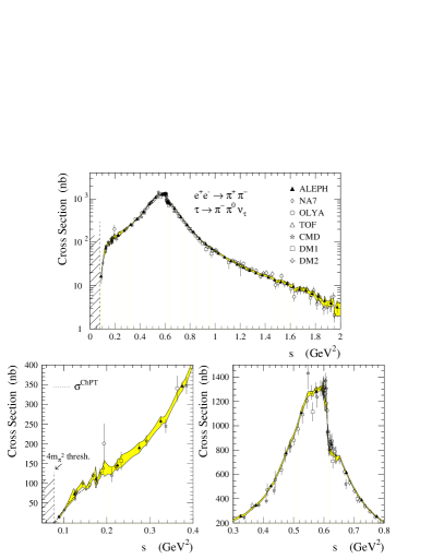
Figure 1: Two-pion cross section as a function of the c.m. energy-squared. The band represents the result of the averaging procedure described in the text within the diagonal errors. The lower left hand plot shows the chiral expansion of the two-pion cross section used (see Ref. [1]).

Results

With the inclusion of the $\tau$ vector spectral functions, the hadronic contributions to $\alpha(M_{\rm Z}^{2})$ and to $a_{\mu}$ are found to be [1]

$$\Delta\alpha_{\rm had}(M_{\rm Z}^{2}) = (281.0\pm 6.2)\times 10^{-4}~{},$$

$$a_{\mu}^{\rm had} = (701.1\,\pm\,9.4)\times 10^{-10}~{},$$ (11)

with an improvement for $a_{\mu}^{\rm had}$ of about $40\%$ compared to the previous evaluation (4), while there is only a marginal improvement of $\Delta\alpha(M_{\rm Z}^{2})$ for which the dominant uncertainties stem from higher energies.

(II) Extended theoretical approach

The above analysis shows that in order to improve the precision on $\Delta\alpha(M_{\rm Z}^{2})$, a more accurate determination of the hadronic cross section between 2 GeV and 10 GeV is needed. On the experimental side there are ongoing $R$ measurements performed by the BES Collaboration [19]. On the other hand, QCD analyses using hadronic $\tau$ decays performed by ALEPH [20] and recently by OPAL [21] revealed excellent applicability of the Wilson Operator Product Expansion (OPE) [22] (also called SVZ approach [23]), organizing perturbative and nonperturbative contributions to a physical observable using the concept of global quark-hadron duality, at the scale of the $\tau$ mass, $M_{\tau}\simeq 1.8~{}{\rm GeV}$. Using moments of spectral functions, dimensional nonperturbative operators contributing to the $\tau$ hadronic width have been fitted simultaneously and turned out to be small. This encouraged the authors of Ref. [24] to apply a similar approach based on spectral moments to determine the size of the nonperturbative contributions to integrals over total cross sections in $e^{+}e^{-}$ annihilation, and to figure out whether or not the OPE, i.e., global duality is a valid approach at relatively low energies.

Theoretical prediction of $R(s)$

The optical theorem relates the total hadronic cross section in $e^{+}e^{-}$ annihilation, $R(s_{0})$, at a given energy-squared, $s_{0}$, to the absorptive part of the photon vacuum polarization correlator

$$R(s_{0})=12\pi{\rm Im}\Pi(s_{0}+i\epsilon)~{}.$$ (12)

Perturbative QCD predictions up to next-to-next-to leading order ($\alpha_{s}^{3}$) as well as second order quark mass corrections far from the production threshold and the first order dimension $D=4$ nonperturbative term are available for the Adler $D$-function [25], which is the logarithmic derivative of the correlator $\Pi$, carrying all physical information:

$$D(s)=-12\pi^{2}s\frac{d\Pi(s)}{ds}~{}.$$ (13)

This yields the relation

$$R(s_{0})=\frac{1}{2\pi i}\oint\limits_{|s|=s_{0}}\frac{ds}{s}D(s)~{},$$ (14)

where the contour integral runs counter-clockwise around the circle from $s=s_{0}+i\epsilon$ to $s=s_{0}-i\epsilon$. The Adler function is given by [26, 27, 28]

$$D_{f_{i}}(-s)=N_{C}\sum_{f}Q_{f}^{2}\Bigg{\{}$$ (15)

$$1+d_{0}\,a_{s}+d_{1}\,a_{s}^{2}+\tilde{d}_{2}\,a_{s}^{3}$$

$$-\;\frac{m_{f}^{2}(s)}{s}\left(6+28\,a_{s}+(295.1-12.3\,n_{f})\,a_{s}^{2}\right)$$

$$+\;\frac{2\pi^{2}}{3}\left(1-\frac{11}{18}\,a_{s}\right)\frac{\left\langle\frac{\alpha_{s}}{\pi}GG\right\rangle}{s^{2}}$$

$$+\;8\pi^{2}\left(1-a_{s}\right)\frac{\langle m_{f}\bar{q_{f}}q_{f}\rangle}{s^{2}}$$

$$+\;\frac{32\pi^{2}}{27}a_{s}\sum_{k}\frac{\langle m_{k}\bar{q_{k}}q_{k}\rangle}{s^{2}}$$

$$+\;12\pi^{2}\frac{\langle{\cal O}_{6}\rangle}{s^{3}}\;+\;16\pi^{2}\frac{\langle{\cal O}_{8}\rangle}{s^{4}}\Bigg{\}}~{},$$

where additional logarithms occur when $\mu^{2}\neq s$, $\mu$ being the renormalization scale and $a_{s}=\frac{\alpha_{s}(s)}{\pi}$. The coefficients of the massless perturbative part are $d_{0}=1$, $d_{1}=1.9857-0.1153\,n_{f}$, $\tilde{d}_{2}=d_{2}+\beta_{0}^{2}\pi^{2}/48$ with $\beta_{0}=11-2n_{f}/3$, $d_{2}=-6.6368-1.2001\,n_{f}-0.0052\,n_{f}^{2}-1.2395\,(\sum_{f}Q_{f})^{2}/N_{C}\sum_{f}Q_{f}^{2}$ and $n_{f}$ being the number of involved quark flavours. The nonperturbative operators in Eq. (15) are the gluon condensate, $\langle(\alpha_{s}/\pi)GG\rangle$, and the quark condensates, $\langle m_{f}\bar{q_{f}}q_{f}\rangle$. The latter obey approximately the PCAC relations

$$(m_{u}+m_{d})\langle\bar{u}u+\bar{d}d\rangle \simeq -2f_{\pi}^{2}m_{\pi}^{2}~{},$$

$$m_{s}\langle\bar{s}s\rangle \simeq -f_{\pi}^{2}(m_{K}^{2}-m_{\pi}^{2})~{},$$ (16)

with the pion decay constant $f_{\pi}=(92.4\pm 0.26)$ MeV [18]. In the chiral limit the equations $f_{\pi}=f_{K}$ and $\langle\bar{u}u\rangle=\langle\bar{d}d\rangle=\langle\bar{s}s\rangle$ hold. The complete dimension $D=6$ and $D=8$ operators are parametrized phenomenologically in Eq. (15) using the saturated vacuum expectation values $\langle{\cal O}_{6}\rangle$ and $\langle{\cal O}_{8}\rangle$, respectively.

Although the theoretical prediction of $R$ using Eqs. (14) and (15) assumes local duality and therefore suffers from unpredicted low-energy resonance oscillations, the following integration, Eqs. (5)/(7), turns the hypothesis into global duality, i.e., the nonperturbative oscillations are averaged over the energy spectrum. However, a systematic uncertainty is introduced through the cut at explicitly 1.8 GeV so that non-vanishing oscillations could give rise to a bias after integration. The associated systematic error is estimated in Ref. [29] by means of fitting different oscillating curves to the data around the cut region, yielding the error estimates $\Delta(\Delta\alpha_{\rm had}(M_{\rm Z}^{2}))=0.15\times 10^{-4}$ and $\Delta a_{\mu}^{\rm had}=0.24\times 10^{-10}$, from the comparison of the integral over the oscillating simulated data to the OPE prediction. These numbers are added as systematic uncertainties to the corresponding low-energy integrals.

In asymptotic energy regions we use the formulae of Ref. [31] which include complete quark mass corrections up to order $\alpha_{s}^{2}$ to evaluate the perturbative prediction of $R(s)$ entering into the integrals (5) and (7).

Theoretical uncertainties

Details about the parameter errors used to estimate the uncertainties accompanying the theoretical analysis are given in Refs. [24, 29]. Theoretical uncertainties arise from essentially three sources

• The perturbative prediction. The estimation of theoretical errors of the perturbative series is strongly linked to its truncation at finite order in $\alpha_{s}$. This introduces a non-vanishing dependence on the choice of the renormalization scheme and the renormalization scale. Furthermore, one has to worry whether the missing four-loop order contribution $d_{3}\,a_{s}^{4}$ gives rise to large corrections to the perturbative series. An additional uncertainty stems from the ambiguity between the results on $R$ obtained using contour-improved fixed-order perturbation theory ($\rm FOPT_{\rm CI}$) and FOPT only (see Ref. [20]). The value $\alpha_{s}(M_{Z}^{2})=0.1201\pm 0.0020$ is taken, as the average between the results from $\tau$ hadronic decays and the Z hadronic width which have essentially uncorrelated uncertainties [30].

• The quark mass correction. Since a theoretical evaluation of the integrals (5) and (7) is only applied far from quark production thresholds, quark mass corrections and the corresponding errors are small.

• The nonperturbative contribution. In order to detach the measurement from theoretical constraints on the nonperturbative parameters of the OPE, the dominant dimension $D=4,6,8$ terms are determined experimentally by means of a simultaneous fit of weighted integrals over the inclusive low energy $e^{+}e^{-}$ cross section, so-called spectral moments, to the theoretical prediction obtained from Eq. (15). Small uncertainties are introduced from possible deviations from the PCAC relations (4).

The spectral moment fit of the nonperturbative operators results in a very small contribution from the OPE power terms to the lowest moment at the scale of $1.8~{}{\rm GeV}$ (repeated and confirmed at $2.1~{}{\rm GeV}$), as expected from the $\tau$ analyses [20, 21]. The value of $\langle\frac{\alpha_{s}}{\pi}GG\rangle=(0.037\pm 0.019)~{}{\rm GeV}^{4}$ found for the gluon condensate is compatible with other evaluations [32, 33]. The analysis proves that global duality holds at $1.8~{}{\rm GeV}$ and nonperturbative effects contribute only negligibly, so that above this energy perturbative QCD can replace the rather imprecise data in the dispersion integrals (5) and (7).

Results

The $R(s)$ measurements and the corresponding theoretical prediction are shown in Fig. 2. The wide shaded bands indicate the regions where data are used instead of theory to evaluate the dispersion integrals, namely below 1.8 GeV and at $c\bar{c}$ threshold energies. Good agreement between data and QCD is found above 8 GeV, while at lower energies systematic deviations are observed. The $R$ measurements in this region are essentially provided by the $\gamma\gamma 2$ [34] and MARK I [35] Collaborations. MARK I data above 5 GeV lie systematically above the measurements of the Crystal Ball [36] and MD1 [37] Collaborations as well as above the QCD prediction.

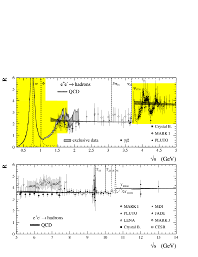
Figure 2: Inclusive hadronic cross section ratio in $e^{+}e^{-}$ annihilation versus the c.m. energy $\sqrt{s}$. Additionally shown is the QCD prediction of the continuum contribution as explained in the text. The shaded areas indicate regions were experimental data are used for the evaluation of $\Delta\alpha_{\rm had}(M_{\rm Z}^{2})$ and $a_{\mu}^{\rm had}$ in addition to the measured narrow resonance parameters. The exclusive $e^{+}e^{-}$ cross section measurements at low c.m. energies are taken from DM1,DM2,M2N,M3N,OLYA,CMD,ND and $\tau$ data from ALEPH (see Ref. [1] for detailed information).

The combination of the theoretical and experimental evaluations of the integrals yields the results [24]

$$\Delta\alpha_{\rm had}(M_{\rm Z}^{2}) = (277.8\pm 2.2_{\rm exp}\pm 1.4_{\rm theo})\times 10^{-4},~{}~{}~{}~{}$$

$$a_{\mu}^{\rm had} = (695.1\pm 7.5_{\rm exp}\pm 0.7_{\rm theo})\times 10^{-10}~{},~{}~{}~{}~{}$$ (17)

with a significant improvement by more than a factor of two for $\Delta\alpha(M_{\rm Z}^{2})$, and a $20\%$ better accuracy on $a_{\mu}^{\rm had}$ compared to the numbers (4).

The authors of Ref. [38] improved the above analysis in the charm region by normalizing experimental results in the theoretically not accessible region (at least locally) so that they match perturbative QCD at safe energies below and above the occurrence of resonances.

The so-renormalized data show excellent agreement among different experiments which supports the hypothesis made that experimental systematic errors are completely correlated over the whole involved energy regime. The result (after correcting for the small top quark contribution) reads [38]

$$\Delta\alpha_{\rm had}(M_{\rm Z}^{2})=(276.7\pm 1.7)\times 10^{-4}~{}.$$ (18)

Another, very elegant method based on an analytical calculation of the unsubtracted dispersion relation, corresponding to the subtracted integral (5), was presented in Ref. [39]. Only the low-energy pole contribution is taken from data, while the contribution from higher energies is calculated analytically using the two-point correlation function given in Ref. [31], and the renormalization group equations for the running quantities. This leads to the precise result [39]

$$\Delta\alpha_{\rm had}(M_{\rm Z}^{2})=(277.2\pm 1.9)\times 10^{-4}~{}.$$ (19)

Both numbers (18) and (19) are in agreement with $\Delta\alpha(M_{\rm Z}^{2})$ from Eq. (4).

(III) Constraints from QCD sum rules

It was shown in Ref. [29] that the previous determinations can be further improved by using finite-energy QCD sum rule techniques in order to access theoretically energy regions where locally perturbative QCD fails. This idea was first presented in Ref. [40]. In principle, the method uses no additional assumption beyond those applied in Section 4. However, parts of the dispersion integrals evaluated at low-energy and the $c\bar{c}$ threshold are obtained from values of the Adler $D$-function itself, for which local quark-hadron duality is assumed to hold. One therefore must perform an evaluation at rather high energies (3 GeV for $u,d,s$ quarks and 15 GeV for the $c$ quark contribution have been chosen in Ref. [29]) to suppress deviations from local duality due to nonperturbative phenomena.

The idea of the approach is to reduce the data contribution to the dispersion integrals by subtracting analytical functions from the singular integration kernels in Eqs. (5) and (7), and adding the subtracted part subsequently by using theory only. Two approaches have been applied in Ref. [29]: first, a method based on spectral moments is defined by the identity

$$F=\int\limits_{4m_{\pi}^{2}}^{s_{0}}\!\!ds\,R(s)\left[f(s)-p_{n}(s)\right]$$ (20)

$$\hskip 17.07182pt+\;\frac{1}{2\pi i}\!\!\oint\limits_{|s|=s_{0}}\!\!\!\frac{ds}{s}\left[P_{n}(s_{0})-P_{n}(s)\right]D_{uds}(s)~{},$$

with $P_{n}(s)=\int_{0}^{s}dt\,p_{n}(t)$ and $f(s)=\alpha(0)^{2}K(s)/(3\pi^{2}s)$ for $F\equiv a_{\mu,\,[2m_{\pi},\;\sqrt{s_{0}}]}^{\rm had}$, as well as $f(s)=\alpha(0)M_{\rm Z}^{2}/(3\pi s(s-M_{\rm Z}^{2}))$ for $F\equiv\Delta\alpha_{\rm had}(M_{\rm Z}^{2})_{[2m_{\pi},\;\sqrt{s_{0}}]}$. The analytic functions $p_{n}(s)$ approximate the kernel $f(s)$ in order to reduce the contribution of the first integral in Eq. (20) which has a singularity at $s=0$ and is thus evaluated using experimental data. The second integral in Eq. (20) can be calculated theoretically in the framework of the OPE. The functions $p_{n}(s)$ are chosen in order to reduce the uncertainty of the data integral. This approximately coincides with a low residual value of the integral, i.e., a good approximation of the integration kernel $f(s)$ by the $p_{n}(s)$ defined as [29]

$$p_{n}(s)\equiv\sum_{i=1}^{n}c_{i}\left(1-\left(\frac{s}{s_{0}}\right)^{\!\!i}\right)~{},$$ (21)

with the form $(1-s/s_{0})$ in order to ensure a vanishing integrand at the crossing of the positive real axis where the validity of the OPE is questioned [23]. Polynomials of order $s^{n}$ involve leading order nonperturbative contributions of dimension $D=2(n+1)$. The analysis is therefore restricted to the linear $n=1$ case only.

A second approach uses the dispersion relation of the Adler $D$-function

$$D_{f}(Q^{2})=Q^{2}\!\!\int\limits_{4m_{f}^{2}}^{\infty}\!\!ds\,\frac{R_{f}(s)}{(s+Q^{2})^{2}}~{},$$ (22)

for space-like $Q^{2}=-q^{2}$ and the quark flavour $f$. The above integrand approximate the integration kernels in Eqs. (5) and (7), so that the modified Eq. (20) reads

$$F=\int\limits_{4m_{\pi}^{2}}^{s_{0}}\!\!ds\,R^{\rm Data}(s)\left[f(s)-\frac{A_{F}Q^{2}}{(s+Q^{2})^{2}}\right]$$ (23)

$$\hskip 14.22636pt+\;A_{F}\left(D_{uds}(Q^{2})-Q^{2}\!\int\limits_{s_{0}}^{\infty}\!ds\,\frac{R_{uds}^{\rm QCD}(s)}{(s+Q^{2})^{2}}\right)~{},$$

with a normalization constant $A_{F}$ to be optimized for both $\Delta\alpha(M_{\rm Z}^{2})$ and $a_{\mu}^{\rm had}$.

In both approaches, a compromise must be obtained between uncertainties of experimental and theoretical origins. As the subtracted contribution increases, the experimental error diminishes as expected. However, this improvement is spoiled by a correspondingly larger theoretical error. The procedure followed is designed to minimize the total uncertainty [29].

Results

A $\chi^{2}$ fit taking into account the experimental and theoretical correlations between the polynomial moments yields for the first (spectral moment) approach (hadronic contribution from $2m_{\pi}$ to 1.8 GeV) [29]

$$\Delta\alpha_{\rm had}(M_{\rm Z}^{2})_{[0,1.8]} = (56.53\pm 0.73_{\rm exp}\pm 0.39_{\rm th})\times 10^{-4}~{},$$

$$a_{\mu,\,[0,1.8]}^{\rm had} = (634.3\pm 5.6_{\rm exp}\pm 2.1_{\rm th})\times 10^{-10}~{},$$

while the dispersion relation approach gives ($\sqrt{Q^{2}}=3~{}{\rm GeV}$) [29]

$$\Delta\alpha_{\rm had}(M_{\rm Z}^{2})_{[0,1.8]} = (56.36\pm 0.70_{\rm exp}\pm 0.18_{\rm th})\times 10^{-4}~{},$$

$$a_{\mu,\,[0,1.8]}^{\rm had} = (632.5\pm 6.2_{\rm exp}\pm 1.6_{\rm th})\times 10^{-10}~{}.$$

Only the most precise of the above numbers are used for the final results. The above theory-improved results can be compared to the corresponding pure experimental values, $\Delta\alpha_{\rm had}(M_{\rm Z}^{2})_{[0,1.8]}=(56.77\pm 1.06)\times 10^{-4}$ and $a_{\mu,\,[0,1.8]}^{\rm had}=(635.1\pm 7.4)\times 10^{-10}$, showing clear improvement.

For the charm threshold region only the approach (23) is used giving for the hadronic contributions from 3.7 GeV to 5 GeV ($\sqrt{Q^{2}}=15~{}{\rm GeV}$) [29]

$$\Delta\alpha_{\rm had}(M_{\rm Z}^{2})_{[3.7,5]} = (24.75\pm 0.84_{\rm exp}\pm 0.50_{\rm th})\times 10^{-4}~{},$$

$$a_{\mu,\,[3.7,5]}^{\rm had} = (14.31\pm 0.50_{\rm exp}\pm 0.21_{\rm th})\times 10^{-10}~{},$$

for which compared with the pure data results, $\Delta\alpha_{\rm had}(M_{\rm Z}^{2})_{[3.7,5]}=(25.04\pm 1.21)\times 10^{-4}$ and $a_{\mu,\,[3.7,5]}^{\rm had}=(14.44\pm 0.62)\times 10^{-10}$, only a slight improvement is observed.

5 FINAL RESULTS

Table 2 shows the experimental and theoretical evaluations of $\Delta\alpha_{\rm had}(M_{\rm Z}^{2})$, $a_{\mu}^{\rm had}$ and $a_{e}^{\rm had}$ for the respective energy regimes. Experimental errors between different lines are assumed to be uncorrelated, whereas theoretical errors, but those from $c\bar{c}$ and $b\bar{b}$ thresholds which are quark mass dominated, are added linearily.

According to Table 2, the combination of the theoretical and experimental evaluations of the integrals (5) and (7) yields the final results

$$\Delta\alpha_{\rm had}(M_{\rm Z}^{2}) = (276.3\pm 1.1_{\rm exp}\pm 1.1_{\rm th})\times 10^{-4}~{},$$

$$\alpha^{-1}(M_{\rm Z}^{2}) = 128.933\pm 0.015_{\rm exp}\pm 0.015_{\rm th}~{},$$ (24)

$$a_{\mu}^{\rm had} = (692.4\pm 5.6_{\rm exp}\pm 2.6_{\rm th})\times 10^{-10}~{},$$

$$a_{\mu}^{\rm SM} = (11\,659\,159.6\pm 5.6_{\rm exp}\pm 3.7_{\rm th})\times 10^{-10}~{},$$

and $a_{e}^{\rm had}=(187.5\pm 1.7_{\rm exp}\pm 0.7_{\rm th})\times 10^{-14}$ for the leading order hadronic contribution to $a_{e}$. The improvement for $\alpha(M_{\rm Z}^{2})$ compared to the previous results (4) amounts to $40\%$ and $a_{\mu}^{\rm had}$ is about $17\%$ more precise than (4).

The total $a_{\mu}^{\rm SM}$ value includes an additional contribution from non-leading order hadronic vacuum polarization summarized in Refs. [41, 1] to be $a_{\mu}^{\rm had}[(\alpha/\pi)^{3}]=(-10.0\pm 0.6)\times 10^{-10}$. Also the light-by-light scattering (LBLS) contribution has recently been reevaluated in Refs. [42] and [43] of which the average $\langle a_{\mu}^{\rm had}[{\rm LBLS}]\rangle=(-8.5\pm 2.5)\times 10^{-10}$ is used here.

Figure 3 shows a compilation of published results for the hadronic contributions to $\alpha(M_{\rm Z}^{2})$ and $a_{\mu}$. Some authors give the contribution for the five light quarks only and add the top quark part separately. This has been corrected for in Fig. 3.

6 THE MASS OF THE STANDARD MODEL HIGGS BOSON

The new precise result (5) for $\alpha(s)$ is exploited to repeat the global electroweak fit in order to adjust the mass of the Standard Model Higgs boson, $M_{H}$. The corresponding uncertainty on ${\rm sin}^{2}\theta_{\rm W}$ now reaches $5\times 10^{-4}$, well below the experimental accuracy on this quantity and on $m_{t}$ (see Table 1). The prediction of the Standard Model is obtained from the ZFITTER electroweak library [52] and the experimental input is taken from the latest review [6]. The standard value [2] of $\alpha(s)$ yields

$$log(M_{H}) = 1.92^{+0.32}_{-0.41}~{},$$

$$M_{H} = (84^{+91}_{-51})~{}{\rm GeV/c}^{2}~{},$$ (25)

while the improved determination (5) provides

$$log(M_{H}) = 2.02^{+0.23}_{-0.25}~{},$$

$$M_{H} = (105^{+73}_{-46})~{}{\rm GeV/c}^{2}~{}.$$ (26)

Table 2: Contributions to $\Delta\alpha_{\rm had}(M_{\rm Z}^{2})$, $a_{\mu}^{\rm had}$ and to $a_{e}^{\rm had}$ from the different energy regions. The subscripts in the first column give the quark flavours involved in the calculation.

Energy (GeV)	$\Delta\alpha_{\rm had}(M_{\rm Z}^{2})\times 10^{4}$	$a_{\mu}^{\rm had}\times 10^{10}$	$a_{e}^{\rm had}\times 10^{14}$
$(2m_{\pi}$ – $1.8)_{uds}$	$56.36\pm 0.70_{\rm exp}\pm 0.18_{\rm th}$	$634.3\pm 5.6_{\rm exp}\pm 2.1_{\rm th}$	$173.67\pm 1.7_{\rm exp}\pm 0.6_{\rm th}$
$(1.8$ – $3.700)_{uds}$	$24.53\pm 0.28_{\rm th}$	$33.87\pm 0.46_{\rm th}$	$8.13\pm 0.11_{\rm th}$
$\psi(1S,2S,3770)_{c}$ $+~{}(3.7$ – $5)_{udsc}$	$24.75\pm 0.84_{\rm exp}\pm 0.50_{\rm th}$	$14.31\pm 0.50_{\rm exp}\pm 0.21_{\rm th}$	$3.41\pm 0.12_{\rm exp}\pm 0.05_{\rm th}$
$(5$ – $9.3)_{udsc}$	$34.95\pm 0.29_{\rm th}$	$6.87\pm 0.11_{\rm th}$	$1.62\pm 0.03_{\rm th}$
$(9.3$ – $12)_{udscb}$	$15.70\pm 0.28_{\rm th}$	$1.21\pm 0.05_{\rm th}$	$0.28\pm 0.02_{\rm th}$
$(12$ – $\infty)_{udscb}$	$120.68\pm 0.25_{\rm th}$	$1.80\pm 0.01_{\rm th}$	$0.42\pm 0.01_{\rm th}$
$(2m_{t}$ – $\infty)_{t}$	$-0.69\pm 0.06_{\rm th}$	$\approx 0$	$\approx 0$
$(2m_{\pi}$ – $\infty)_{udscbt}$	$276.3\pm 1.1_{\rm exp}\pm 1.1_{\rm th}$	$692.4\pm 5.6_{\rm exp}\pm 2.6_{\rm th}$	$187.5\pm 1.7_{\rm exp}\pm 0.7_{\rm th}$

Figure 3: Comparison of $\Delta\alpha_{\rm had}(M_{\rm Z}^{2})$ and $a_{\mu}^{\rm had}$ evaluations. The values for $\Delta\alpha_{\rm had}(M_{\rm Z}^{2})$ are taken from Refs. [44, 2, 45, 46, 47, 1, 24, 38, 39, 29], while those for $a_{\mu}^{\rm had}$ are from Refs. [48, 49, 50, 2, 51, 1, 24, 29].

Considering the direct Higgs search currently conducted at CERN by the four LEP experiments, it is worth remarking that the $21~{}{\rm GeV/c}^{2}$ shift between the two indirect determinations is almost entirely due to the region 2.0 - 3.7 GeV in the evaluation of $\Delta\alpha_{\rm had}(s)$ where the available $e^{+}e^{-}$ data are systematically higher than the QCD prediction (see Fig. 2). In this respect, the preliminary results from BES [19], which are more precise than the earlier measurements in this energy range, are observed to nicely agree with QCD. We are looking forward to more complete and more precise results in this crucial energy region.

7 SUMMARIZING THE PROCEDURE AND ITS JUSTIFICATION

We have described a three-step procedure to improve the evaluation of hadronic vacuum polarisation occuring in the anomalous magnetic moments of the leptons and the running of $\alpha$. By far the most rewarding step was to replace poor experimental data on $e^{+}e^{-}$ annihilation cross sections in the 1.8 - 3.7 GeV range and above 5 GeV by a precise QCD prediction. The justification for believing this prediction at the level quoted ($\sim 1\%$) follows from direct tests using experimental data.

The two assumptions needed for applying QCD to this problem are: (i) $R(s)$ can be approximated by $R_{QCD}(s)$ in an average sense only since an integral is computed (global quark-hadron duality) and (ii) perturbative QCD can be reliably used at energies as low as 1.8 GeV.

These hypotheses have been thoroughly tested in the study of hadronic $\tau$ decays [20, 21] for the dominant isovector amplitude, integrating from threshold to 1.8 GeV. Using the precise measurement of $R_{\tau,V+A}$ and moments of the corresponding spectral function, the nonperturbative contributions were found to be smaller than $1\%$, thus enabling to validate the perturbative QCD prediction from 1.8 down to 1.0 GeV. Over this range, the precision of the test reaches $\sim 1\%$, going down to $\sim 2\%$ near 1 GeV. The consistency of the QCD description can be expressed through the values of $\alpha_{s}(M_{Z}^{2})$ found in the different cases studied: $0.1202\pm 0.0008_{exp}\pm 0.0024_{th}\pm 0.0010_{evol}$ for ($V+A\,,I=1$), $0.1197\pm 0.0018$ for ($V\,,I=1$), $0.1207\pm 0.0017$ for ($A\,,I=1$) in $\tau$ decays [20], and $0.1205\pm 0.0053$ for ($V\,,I=0,1$) in $e^{+}e^{-}$ annihilation [24].

In essence, the nice properties (quark-hadron duality and validity of perturbative QCD calculations) observed in an a priori critical energy region are applied at higher and safer energies, where the achieved precision should be $1\%$ or better.

8 CONCLUSIONS

This note summarizes the recent effort that has been undertaken in order to ameliorate the theoretical predictions for $\alpha(M_{\rm Z}^{2})$ and $a_{\mu}^{\rm had}$, crucially necessary to maintain the sensitivity of the diverse experimental improvements on the Standard Model Higgs mass, on the one hand, and tests of the electroweak theory on the other hand. The new value of $\alpha^{-1}(M_{\rm Z}^{2})=128.933\pm 0.021$ for the running fine structure constant is now sufficiently accurate so that its precision is no longer a limitation in the global Standard Model fit. On the contrary, more effort is needed to further improve the precision of the hadronic contribution to the anomalous magnetic moment of the muon below the intended experimental accuracy of BNL-E821 [4], which is about $4\times 10^{-10}$. Fortunately, new low energy data are expected in the near future from $\tau$ decays (CLEO, OPAL, DELPHI, BaBar) and from $e^{+}e^{-}$ annihilation (BES, CMD II, DA$\Phi$NE). Additional support might come from the theoretical side using chiral perturbation theory to access the low energy inverse moment sum rules (5) and (7). One could, e.g., apply a similar procedure as the one which was used in Ref. [53] to determine the constant $L_{10}$ of the chiral lagrangian.

References

- [1] R. Alemany, M. Davier and A. Höcker, Europ. Phys. J. C2 (1998) 123
- [2] S. Eidelman and F. Jegerlehner, Z. Phys. C67 (1995) 585
-
[3]
J. Bailey et al.,
Phys. Lett. B68 (1977) 191.
F.J.M. Farley and E. Picasso, “The muon Experiments”, Advanced Series on Directions in High Energy Physics - Vol. 7 Quantum Electrodynamics, ed. T. Kinoshita, World Scientific 1990 - [4] B. Lee Roberts, Z. Phys. C56 (Proc. Suppl.) (1992) 101
- [5] C. Timmermans, Talk given at the International Conference on High Energy Physics, Vancouver (1998)
- [6] D. Karlen, Talk given at the International Conference on High Energy Physics, Vancouver (1998)
- [7] R. Partridge, Talk given at the International Conference on High Energy Physics, Vancouver (1998)
-
[8]
G. Degrassi, P. Gambino, M. Passera and A. Sirlin,
Phys. Lett. B418 (1998) 209;
G. Degrassi, Talk given at the Zeuthen Workshop on Elementary Particle Theory: Loops and Legs in Gauge Theories, Rheinsberg, Germany (1998), hep-ph/9807293 - [9] M. Steinhauser, “Leptonic contribution to the effective electromagnetic coupling constant up to three loops”, Report MPI/PhT/98-22 (1998)
- [10] N. Cabibbo and R. Gatto, Phys. Rev. Lett. 4 (1960) 313; Phys. Rev. 124 (1961) 1577.
- [11] A. Czarnecki, B. Krause and W.J. Marciano, Phys. Rev. Lett. 76 (1995) 3267; Phys. Rev. D52 (1995) 2619
- [12] S. Peris, M. Perrottet and E. de Rafael, Phys. Lett. B355 (1995) 523
- [13] R. Jackiw and S. Weinberg, Phys. Rev. D5 (1972) 2473
- [14] M. Gourdin and E. de Rafael, Nucl. Phys. B10 (1969) 667
- [15] S.J. Brodsky and E. de Rafael, Phys. Rev. 168 (1968) 1620
- [16] ALEPH Collaboration (R. Barate et al.) Z. Phys. C76 (1997) 15
-
[17]
S. Tisserant and T.N. Truong,
Phys. Lett. B115 (1982) 264;
A. Pich, Phys. Lett. B196 (1987) 561;
H. Neufeld and H. Rupertsberger, Z. Phys. C68 (1995) 91 - [18] C. Caso et al. (Particle Data Group),Europ. Phys. J. C3 (1998) 1
- [19] Z. Zhao, Talk given at the International Conference on High Energy Physics, Vancouver (1998)
- [20] ALEPH Collaboration (R. Barate et al.), Eur. Phys. J. C4 (1998) 409
- [21] OPAL Collaboration (K. Ackerstaff et al.), “Measurement of the Strong Coupling Constant and the Vector and Axial-Vector Spectral Functions in Hadronic Tau Decays”, CERN-EP/98-102 (1998)
- [22] K.G. Wilson, Phys. Rev. 179 (1969) 1499
- [23] M.A. Shifman, A.L. Vainshtein and V.I. Zakharov, Nucl. Phys. B147 (1979) 385, 448, 519
- [24] M. Davier and A. Höcker, Phys. Lett. B419 (1998) 419
- [25] S. Adler, Phys. Rev. D10 (1974) 3714
-
[26]
L.R. Surguladze and M.A. Samuel,
Phys. Rev. Lett. 66 (1991) 560;
S.G. Gorishny, A.L. Kataev and S.A. Larin, Phys. Lett. B259 (1991) 144 - [27] S.G. Gorishny, A.L. Kataev and S.A. Larin, Il Nuovo Cim. 92A (1986) 119
- [28] E. Braaten, S. Narison and A. Pich, Nucl. Phys. B373 (1992) 581
- [29] M. Davier and A. Höcker, “New Results on the Hadronic Contribution to and to ”, Report LAL 98-38 (1998), to be published in Phys. Lett.
- [30] M. Davier, “New Results on and ”, Report LAL 98-53 (1998), to be published in the Proceedings of the Rencontres de Moriond “Electroweak Interactions and Unified Theories” Les Arcs, France, March 14-21, 1998
- [31] K.G. Chetyrkin, J.H. Kühn and M. Steinhauser, Nucl. Phys. B482 (1996) 213
- [32] L.J. Reinders, H. Rubinstein and S. Yazaki, Phys. Rep. 127 (1985) 1
- [33] R.A. Bertlmann, Z. Phys. C39 (1988) 231
- [34] C. Bacci et al. ( Collaboration), Phys. Lett. B86 (1979) 234
- [35] J.L. Siegrist et al. (MARK I Collaboration), Phys. Rev. D26 (1982) 969
-
[36]
Z. Jakubowski et al. (Crystal Ball Collaboration),
Z. Phys. C40 (1988) 49;
C. Edwards et al. (Crystal Ball Collaboration), SLAC-PUB-5160 (1990) -
[37]
A.E. Blinov et al. (MD-1 Collaboration),
Z. Phys. C49 (1991) 239;
A.E. Blinov et al. (MD-1 Collaboration), Z. Phys. C70 (1996) 31 - [38] J.H. Kühn and M. Steinhauser, “A theory driven analysis of the effective QED coupling at ”, MPI-PHT-98-12 (1998)
- [39] J. Erler, “ Scheme Calculation of the QED Coupling ”, UPR-796-T (1998)
- [40] S. Groote, J.G. Körner, N.F. Nasrallah and K. Schilcher, “QCD Sum Rule Determination of with Minimal Data Input”, Report MZ-TH-98-02 (1998)
- [41] B. Krause, Phys. Lett. B390 (1997) 392
- [42] M. Hayakawa, T. Kinoshita, Phys. Rev. D57 (1998) 465
- [43] J. Bijnens, E. Pallante and J. Prades, Nucl. Phys. B474 (1996) 379
- [44] B.W. Lynn, G. Penso and C. Verzegnassi, Phys. Rev. D35 (1987) 42
- [45] H. Burkhardt and B. Pietrzyk, Phys. Lett. B356 (1995) 398
- [46] A.D. Martin and D. Zeppenfeld, Phys. Lett. B345 (1995) 558
- [47] M.L. Swartz, Phys. Rev. D53 (1996) 5268
- [48] L.M. Barkov et al. (OLYA, CMD Collaboration), Nucl. Phys. B256 (1985) 365
- [49] T. Kinoshita, B. Nižić and Y. Okamoto, Phys. Rev. D31 (1985) 2108
- [50] J.A. Casas, C. López and F.J. Ynduráin, Phys. Rev. D32 (1985) 736
- [51] D.H. Brown and W.A. Worstell, Phys. Rev. D54 (1996) 3237
- [52] D. Bardin et al., “Reports of the working group on precision calculations for the Z resonance”, CERN-PPE 95-03
- [53] M. Davier, L. Girlanda, A. Höcker and J. Stern, “Finite Energy Chiral Sum Rules and Tau Spectral Functions”, IPNO-TH-98-05, LAL-98-05, hep-ph/9802447, to be published in Phys. Rev. D