$F_{2}$ at low $Q^{2}$

Abstract

We analyse the data for the proton structure function $F_{2}$ over the entire $Q^{2}$ domain, including especially low $Q^{2}$, in terms of perturbative and non-perturbative QCD contributions. The small distance configurations are given by perturbative QCD, while the large distance contributions are given by the vector dominance model and, for the higher mass $q\overline{q}$ states, by the additive quark approach.

1 INTRODUCTION

There now exist high precision deep inelastic $ep$ scattering data [1, 2] covering both the low $Q^{2}$ and high $Q^{2}$ domains, as well as measurements of the photoproduction cross section. The interesting structure of these measurements, in particular the change in the behaviour of the cross section with $Q^{2}$ at $Q^{2}\sim 0.2{\rm GeV}^{2}$, highlight the importance of obtaining a theoretical QCD description which smoothly links the non-perturbative and perturbative domains.

In any QCD description of a $\gamma^{*}p$ collision, the first step is the conversion of the initial photon into a $q\overline{q}$ pair, which is then followed by the interaction of the pair with the target proton, see Fig.1. Let $\sigma(s,Q^{2})$ be the total cross section for the process $\gamma^{*}p\rightarrow X$ where $Q^{2}$ is the virtuality of the photon and $\sqrt{s}$ is the $\gamma^{*}p$ centre-of-mass energy. We can write the dispersion relation in the following way:

$${\scriptstyle\sigma(s,Q^{2})\;=\;\sum_{q}\>\int_{0}^{\infty}\>\frac{dM^{2}}{(M^{2}+Q^{2})^{2}}\;\rho(s,M^{2})\>\sigma_{q\overline{q}+p}(s,M^{2})}$$ (1)

where the spectral function $\rho(s,M^{2})$ is the density of $q\overline{q}$ states. Following [3] we may divide the integral into two parts: the region $M^{2}<Q_{0}^{2}$ described by the vector meson dominance model (VDM) and the region $M^{2}>Q_{0}^{2}$ described by perturbative QCD. To exploit further this idea we must achieve a better separation between the short and long distance contributions. To do this we take a two-dimensional integral over the longitudinal ($z$), and transverse momentum ($k_{T}$) components of the quark, see Fig1.

The contribution coming from the small mass region is pure VDM. The part which comes from large $k_{T}$ of the quark can be calculated by perturbative QCD in terms of the known parton distributions, whereas for small $k_{T}$ we will use the additive quark model and the impulse approximation. That is only one quark interacts with the target and the quark-proton cross section is well approximated by one third of the proton-proton cross section.

2 The $\gamma^{*}p$ cross section

The spectral function $\rho$ occurring in (1) may be expressed in terms of the $\gamma^{*}\rightarrow q\overline{q}$ matrix element $\cal{M}$. We have $\rho\>\propto|{\cal M}|^{2}$ and in terms of the quark momentum variables $z$ and $k_{T}^{2}$ the cross section in equation (1) becomes

$${\scriptstyle\sigma_{T}=\sum_{q}\alpha\frac{e_{q}^{2}}{4\pi^{2}}\sum_{\lambda\>=\>\pm\>1}\int dzd^{2}k_{T}({\cal M}_{T}{\cal M}_{T}^{*})N_{c}\frac{1}{s}{\rm Im}A_{q\overline{q}+p}}$$

$${\scriptstyle=\sum_{q}\alpha\frac{e_{q}^{2}}{2\pi}\int dzdk_{T}^{2}\frac{[z^{2}+(1-z)^{2}]k_{T}^{2}+m_{q}^{2}}{(\overline{Q}^{2}+k_{T}^{2})^{2}}N_{c}\sigma_{q\overline{q}+p}(k_{T}^{2})}$$ (2)

where the number of colours $N_{c}=3$, and $e_{q}$ is the charge of the quark in units of $e$.

To determine $F_{2}(x,Q^{2})$ at low $Q^{2}$ we have to evaluate the contributions to $\sigma_{T}$ coming from the various kinematic domains. First the contribution from the perturbative domain with $M^{2}>Q_{0}^{2}$ and large $k_{T}^{2}$, and second from the non-perturbative or long-distance domains.

Figure 1: The schematic representation of the ouble dispersion 1 for the $\gamma^{*}p$ total cross section. The cut variables $M$ and $M^{\prime}$ are the invariant masses of the incoming and outgoing $q\bar{q}$ states.

2.1 The $\gamma^{*}p$ cross section in the perturbative domain

We have to include two graphs, one shown on Fig.2 and the diagonal one, for our calculation of the cross section in the perturbative domain. Our formula for the cross section has the following form:

$$\sigma_{T,L}=F_{T,L}(z,k_{1T},l_{T},Q^{2})\otimes f(x,l_{T}^{2})$$ (3)

where

$$f(x,l_{T}^{2})=x\partial g(x,l_{T}^{2})/\partial\ln l_{T}^{2}$$ (4)

is the unintegrated gluon distribution function. The $\otimes$ denotes the convolution in the quark ($z$,$k_{1T}$) and gluon ( $l_{T}$ ) momenta variables. The $F_{T,L}(z,k_{1T},l_{T},Q^{2})$ is the photon-gluon impact factor which can be calculated perturbatively. From the formal point of view the integrals over $l_{T}^{2}$ and $k_{T}^{2}$ cover the interval 0 to $\infty$. For the $l_{T}^{2}$ integration in the domain $l_{T}^{2}<l_{0}^{2}\sim 1{\rm GeV}^{2}$ we may use the approximation

$$\alpha_{S}(l_{T}^{2})\>f(x,l_{T}^{2})\;=\;\frac{l_{T}^{2}}{l_{0}^{2}}\>\alpha_{S}(l_{0}^{2})\;f(x,l_{0}^{2}).$$ (5)

The $f(x,l_{0}^{2})$ is the input gluon distribution with free parameters which can be adjusted to fit the data.

2.2 Calculating the gluon distribution

To calculate the perturbative contributions we need to know the unintegrated gluon distribution $f(x,l_{T}^{2})$. To determine it we carry out the full programme described in detail in Ref. [4]. We solve a “unified” equation for $f(x,l_{T}^{2})$ which incorporates BFKL and DGLAP evolution on an equal footing, and allows the description of both small and large $x$ data. To be precise we solve a coupled pair of integral equations for the gluon and sea quark distributions, as well as allowing for the effects of valence quarks.

Schematically we can write these equations in the following form:

$$f=f^{0}+\overbrace{K_{\scriptscriptstyle BFKL}\otimes f}^{\mathrm{BFKL\;part}}+\overbrace{(P_{gg}-1)\otimes f}^{\mathrm{DGLAP\;part}}+P_{qg}\otimes S$$

$$S=S^{0}+\underbrace{S_{\scriptscriptstyle BOX}\otimes f}_{\mathrm{k_{T}\;factorisation}}+P_{qq}\otimes S$$ (6)

Following Ref. [4] we appropriately constrain the transverse momenta of the emitted gluons along the BFKL ladder. There is an indication, from comparing the size of the next-to-leading $\ln(1/x)$ contribution [5] to the BFKL intercept with the effect due to the kinematic constraint [6], that the incorporation of the constraint into the evolution analysis gives a major part of the subleading $\ln(1/x)$ corrections.

Figure 2: The quark-proton interaction via two gluon exchange

As in Ref. [4] we take $l_{0}^{2}=1$ GeV², but due to the large anomalous dimension of the gluon the results are quite insensitive to the choice of $l_{0}$ in the interval 0.8–1.5 GeV.

The starting distributions for the evolution are specified in terms of three parameters $N,\lambda$ and $\beta$ of the gluon

$$f_{0}(x,l_{0}^{2})\;=\;Nx^{-\lambda}(1-x)^{\beta}$$ (7)

where $l_{0}^{2}=1$ GeV². The input for the quark sea has the following form:

$$S_{u}^{\rm np}\;=\;S_{d}^{\rm np}\;=\;2S_{s}^{\rm np}\;=\;C\>x^{-0.08}(1-x)^{8}.$$ (8)

3 The $\gamma^{*}p$ cross section in the non-perturbative domain

There are two different non-perturbative contributions. For $M^{2}<Q_{0}^{2}$ we use the conventional vector meson formulae whereas for $M^{2}>Q_{0}^{2}$ and $k_{T}^{2}<k_{0}^{2}$ we use the additive quark model and the impulse approximation.

3.1 Vector meson dominance part

As was already mentioned we assume the vector meson dominance model to be valid in the region where $M^{2}<Q_{0}^{2}$, and $Q_{0}^{2}\sim 1.5\;GeV^{2}$. We include three resonances: $\rho,\omega,\phi$. For completness we should also include longitudinal structure function $F_{L}(x,Q^{2})$. $F_{L}$ is given by a formula just like (7) but with the introduction of an extra factor $\xi Q^{2}/M_{V}^{2}$ on the right-hand side. $\xi(Q^{2})$ is a phenomenological function which should decrease with increasing $Q^{2}$. The data for $\rho$ production indicate that $\xi(m_{\rho}^{2})\lower 3.01385pt\hbox{$\;\stackrel{{\scriptstyle\textstyle<}}{{\sim}}\;$}0.7$ [7], whereas at large $Q^{2}$ the usual properties of deep inelastic scattering predict that

$$\frac{F_{L}}{F_{T}}\;\sim\;\frac{4k_{T}^{2}}{Q^{2}}\;\lower 3.01385pt\hbox{$\;\stackrel{{\scriptstyle\textstyle<}}{{\sim}}\;$}\;\frac{M_{V}^{2}}{Q^{2}}.$$ (9)

So throughout the whole $Q^{2}$ region the contribution of $F_{L}$ is less than that of $F_{T}$. In order to calculate $F_{L}$ (VDM) we multiply the VDM prescription for $F_{T}$ with the factor $\xi Q^{2}/M_{V}^{2}$ and use an interpolating formula for $\xi$

$$\xi\;=\;\xi_{0}\left(\frac{M_{V}^{2}}{M_{V}^{2}+Q^{2}}\right)^{2}$$ (10)

with $\xi_{0}=0.7$.

3.2 Additive quark model and the impulse approximation

For large produced masses, $M^{2}>Q_{0}^{2}$ but low quark momenta, $k_{T}^{2}<k_{0}^{2}$ we use the additive quark model and the impulse approximation. Our formulae have the following form:

$$\scriptstyle{\sigma_{T}^{\rm AQM}=\alpha\sum_{q}\frac{e_{q}^{2}}{2\pi}\int dzdk_{T}^{2}\frac{[z^{2}+(1-z)^{2}]k_{T}^{2}+m_{q}^{2}}{(\tilde{Q}^{2}+k_{T}^{2})^{2}}N_{c}\sigma_{q\overline{q}+p}(W^{2})}$$

$$\scriptstyle{\sigma_{L}^{\rm AQM}=\alpha\sum_{q}\frac{e_{q}^{2}}{2\pi}\int dzdk_{T}^{2}\frac{4Q^{2}z^{2}(1-z)^{2}}{(\tilde{Q}^{2}+k_{T}^{2})^{2}}N_{c}\sigma_{q\overline{q}+p}(W^{2})}$$ (11)

where for $\sigma_{q\overline{q}+p}$ we take, for the light quarks,

$$\sigma_{q\overline{q}+p}\>(W^{2})\;=\;\frac{2}{3}\;\sigma_{p\overline{p}}\>(s=\textstyle{\frac{3}{2}}W^{2}).$$ (12)

To allow for the confinement we replaced $\overline{Q}^{2}$ by $\tilde{Q}^{2}=\overline{Q}^{2}+\mu^{2}$ in (11), where $\mu$ is typically the inverse pion radius. We therefore take $\mu^{2}=0.1{\rm GeV}^{2}$. This change has no effect for $Q^{2}\gg\mu^{2}$ but for $Q^{2}\lower 3.01385pt\hbox{$\;\stackrel{{\scriptstyle\textstyle<}}{{\sim}}\;$}\mu^{2}$ it gives some suppression of the AQM contribution.

3.3 The quark mass

In the perturbative QCD domain we use the (small) current quark mass $m_{{\rm curr}}$, while for the long distance contributions it is more natural to use the constituent quark mass $M_{0}$. To provide a smooth transition between these values (in both the AQM and perturbative QCD domains) we take the running mass obtained from a QCD-motivated model of the spontaneous chiral symmetry breaking in the instanton vacuum [8]

$$m_{q}^{2}\;=\;M_{0}^{2}\>\left(\frac{\Lambda^{2}}{\Lambda^{2}+2\mu^{2}}\right)^{6}\>+\>m_{\rm curr.}^{2}.$$ (13)

The parameter $\Lambda=6^{1/3}/\rho=1.09$ GeV, where $\rho=1/(0.6~{}{\rm GeV})$ is the typical size of the instanton. $\mu$ is the natural scale of the problem, that is $\mu^{2}=z(1-z)Q^{2}+k_{T}^{2}$ or $\mu^{2}=z(1-z)Q^{2}+(\mbox{\boldmath$l$}_{T}+\mbox{\boldmath$k$}_{T})^{2}$ as appropriate. For constituent and current quark masses we take $M_{0}=0.35$ GeV and $m_{\rm curr}=0$ for the $u$ and $d$ quarks, and $M_{0}=0.5$ GeV and $m_{\rm curr}=0.15$ GeV for the $s$ quarks.

4 Summary

We have made a fit of the $\sigma_{\gamma^{*}p}$ over the entire range of $Q^{2}$ values. It relies only on the form of the initial gluon distribution see 7 and the boundary between perturbative and non-perturbative contributions. The advantage of our treatment is that we use a full set of integro-differential BFKL and DGLAP equations. These equations are valid over the entire perturbative region. We have used very few free parameters which are used to parametrise the non-perturbative region. We use VDM which is well established in this region. We have used running mass prescription in our calculation. The growth of $m_{q}$ in the transition region is an important non-perturbative effect which we find is required by the $F_{2}$ data.

The full and complete calculation of the cross section together with the longitudinal part is given in [9].

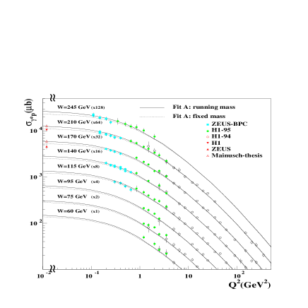
Figure 3: The curves show the virtual photon-proton cross section as a function of $Q^{2}$ for various values of the energy $W$

Acknowledgements MGR thanks the Royal Society, INTAS (95-311) and the Russian Fund of Fundamental Research (98 02 17629), for support. AMS thanks the Polish State Committee for Scientific Research (KBN) grants No. 2 P03B 089 13 and 2 P03B 137 14 for support. Also this work was supported in part by the EU Fourth Framework Programme ‘Training and Mobility of Researchers’, Network ‘Quantum Chromodynamics and the Deep Structure of Elementary Particles’, contract FMRX-CT98-0194 (DG 12 - MIHT).

References

[1] H1 collaboration: C. Adloff et al., Nucl. Phys. B497 (1997) 3;
H1 collaboration: S. Aid et al., Nucl. Phys. B470 (1996) 3.
[2] ZEUS collaboration: J. Breitweg et al., Phys. Lett. B407
(1997) 432.
[3] B. Badelek and J. Kwiecinski, Phys. Lett. B295 (1992) 263.
[4] J. Kwiecinski, A.D. Martin and A.M. Stasto, Phys. Rev. D56 (1997) 3991.
[5] V.S. Fadin and L.N. Lipatov, Phys. Lett. B429 (1998) 127; see also
V.S. Fadin and L.N. Lipatov, contribution to DIS 98, Brussels,
April 1998;
G. Camici and M. Ciafaloni, contribution to DIS 98, Brussels, April 1998.
[6] J. Kwiecinski, A.D. Martin and P.J. Sutton, Z. Phys. C71
(1996) 585.