QCD CALCULATIONS BY NUMERICAL INTEGRATION
Abstract
Calculations in Quantum Chromodynamics are typically performed using a method pioneered by Ellis, Ross and Terrano in 1981. In this method, one combines numerical integrations over the momenta of final state particles with analytical integrations over the momenta of virtual particles. I discuss a more flexible method in which one performs all of the integrations numerically.
1 Introduction
This talk concerns a method for performing perturbative calculations in Quantum Chromodynamics and other quantum field theories. [1] The method may prove useful for cross sections in which one measures something about the hadronic final state, so that one cannot use the powerful but very special methods that apply to completely inclusive quantities like the total cross section for . Examples of such cross sections include jet cross sections in hadron-hadron and lepton-hadron scattering and in .
Many calculations of this kind have been carried out at next-to-leading order in perturbation theory, resulting in an impressive confrontation between theory and experiment. These calculations have been based on a method introduced by Ellis, Ross, and Terrano [2] in the context of . Stated in the simplest terms, one performs some integrations over momenta analytically, others numerically. I shall argue that it is possible instead to do all of these integrations numerically. This has some advantages, principally in the flexibility that it allows.
In this talk, I address specifically the calculation of three-jet-like infrared safe observables in at next-to-leading order, that is order . Examples of such observables include the thrust distribution, the fraction of events that have three jets, and the energy-energy correlation function. There are, of course, several existing computer programs that can calculate any such quantity, the earliest of these being that of Kunszt and Nason, [3] which was developed in 1989. What is new in this talk is not the result achieved, but the method of calculation.
2 The quantity to be calculated.
The order contribution to the observable being calculated has the form
There are, of course, infrared divergences associated with Eq. (2); we understand that an infrared cutoff has been supplied. In Eq. (2), the are the order contributions to the parton level cross section, calculated with zero quark masses. Each contains momentum and energy conserving delta functions. The include ultraviolet renormalization in the MS scheme. The functions describe the measurable quantity to be calculated. Since we calculate a “three-jet” quantity, . The measurement, as specified [4] by the functions , is to be infrared safe: the are smooth functions of the parton momenta and
| (2) |
for . That is, collinear splittings and soft particles do not affect the measurement.
It is convenient to calculate a quantity that is dimensionless. Let us, therefore, define the functions so that they are dimensionless and eliminate the remaining dimensionality in the problem by dividing by , the total cross section at the Born level. We also remove the factor of . Thus, we calculate
| (3) |
3 Setting up the calculation
We note that is a function of the c.m. energy and the renormalization scale . We will choose to be proportional to : . Then depends on . But, because it is dimensionless, it is independent of . This allows us to write
| (4) |
where is any function with
| (5) |
The integration over eliminates the energy conserving delta function in . This is important in allowing cancellations of infrared singularities between contributions with 3- and 4-particle intermediate states to take place. The physical meaning is that, by smearing in the energy , we force the time variables in the two current operators that create the hadronic state to be within of each other. Thus we have a truly short distance problem.
4 The Ellis, Ross, and Terrano method
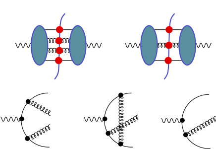
I now describe how one would calculate using the Ellis-Ross-Terrano method. Each partonic cross section in Eq. (2) can be expressed as an amplitude times a complex conjugate amplitude, as illustrated in Fig. 1. One must calculate the amplitudes in dimensions. (In the case of the process , this calculation was performed by Ellis, Ross, and Terrano. [2]) For tree diagrams, the calculation is straightforward. For loop diagrams, this involves an integration, which is performed analytically. The integrals are divergent in four dimensions, so one obtains divergent terms proportional to and in addition to terms that are finite as . Having the amplitudes and complex conjugate amplitudes, one must now multiply by the functions and integrate over the final state parton momenta. These integrations are too complicated to perform analytically, so one must use numerical methods. Unfortunately, the integrals are divergent at . Thus one must split the integrals into two parts. One part can be divergent at but must be simple enough to calculate analytically. The other part can be complicated, but must be convergent at . One calculates the simple, divergent part and cancels the and pole terms against the pole terms coming from the virtual loop diagrams. This leaves the complicated, convergent integration to be performed numerically.
This method is a little bit cumbersome, but it works and has been enormously successful. However it has proven to be difficult to apply the method in the case of two virtual loops. Even with one virtual loop, the method is not very flexible. In modern implementions of the Ellis- Ross-Terrano method, one can easily choose the functions , but any other modification of the integrand requires one to recalculate the amplitudes, and the modification must be simple enough that one can calculate the amplitudes in closed form.
5 Calculation by numerical integration
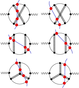
Let us, therefore, inquire whether there is any other way that one might perform such a calculation. We note that the quantity can be expressed in terms of cut Feynman diagrams, as in Fig. 2. Each diagram is a three loop diagram, so we have integrations over loop momenta , and .
5.1 Performing the energy integrations
We first perform the energy integrations. For the graphs in which four parton lines cross the cut, there are four mass-shell delta functions . These delta functions eliminate the three energy integrals over , , and as well as the integral (3) over . For the graphs in which three parton lines cross the cut, we can eliminate the integration over and two of the integrals. One integral over the energy in the virtual loop remains. The integrand contains a product of factors
| (6) |
where is the energy carried by the th propagator around the loop and is the absolute value of the momentum carried on that propagator. We perform the integration by closing the integration contour in the lower half plane. This leads to terms for a virtual point subgraph. In the th term, the propagator energy is set equal to the corresponding and there is a factor . Note that the entire process of performing the energy integrals amounts to some simple algebraic substitutions.
5.2 Cancellations of pinch singularities
Let us denote the contribution to from the cut of graph by . This contribution has the form
| (7) |
where denotes the set of loop momenta . The functions have some singularities, called pinch singularities, that cannot be avoided by deforming the integration contour and some non-pinch singularities that can be avoided by a contour deformation.
Let us consider the pinch singularities, following the analysis of Sterman. [5] The pinch singularities occur when one parton branches into two partons with collinear momenta or when one parton momentum goes to zero. These singularities can lead to logarithmic divergences in the corresponding integral. (There is a complication associated with the terms in gluon self-energy subgraphs but I ignore this complication in this talk.) If we were to calculate the total cross section by using measurement functions in , then the singularities would cancel between the functions associated with the various cuts of the same graph . The underlying reason is unitarity. Now in our case of measured shape variables, the values of corresponding to different cuts are different. This would ruin the cancellation, except that just at the collinear or soft points the functions match. Thus the singularities present in the individual cancel in the sum, . To be precise, the cancellation reduces the strength of the singularity from a strength sufficient to give a logarithmically divergent integral to one that gives a convergent integral.
5.3 Avoiding the non-pinch singularities
The function also has singularities that can be avoided by deforming the integration contours, the non-pinch singularities. These singularities do not cancel, but the Feynman rules provide an prescription that tells us that we should deform the integration contour into the complex plane so as to avoid the singularity. Here deforming the contour means replacing by a complex vector . Then one simply chooses the imaginary part, , of the loop momentum as a function of the real part, , and supplies the appropriate jacobian . Then
| (8) |
5.4 The integration
With the contours appropriately chosen, the integral
| (9) |
is finite. One can simply compute it by Monte Carlo integration after removing from the integration tiny regions near the collinear and soft singular points, where roundoff errors spoil the cancellation of the individual contributions.
Note the significance of putting the summation over cuts inside the integral. When we sum over cuts for a given point in the space of loop momenta, the soft and collinear divergences cancel because the cancellation is built into the Feynman rules. If we were to put the sum over cuts outside the integration, as in the Ellis-Ross-Terrano method, then the individual integrals would be divergent. The calculation would thereby be rendered more difficult.
6 Additional points
Eq. (9) represents the main point of this talk. There are two additional points of principle that I discuss below: renormalization and the special treatment required for self-energy subdiagrams.
6.1 Renormalization
Some of the virtual loop subgraphs are ultraviolet divergent. Normally, one would renormalize these subgraphs by performing loop integrations in space-time dimensions and subtracting the resulting pole term, . Clearly that is not appropriate in a numerical integration. However, one can subtract instead an integral in 4 space-time dimensions such that, in the region of large loop momenta, the integrand of the subtraction term matches the integrand of the subdiagram in question. The integrand of the subtraction term can depend on a mass parameter in such a way that the subtraction term has no infrared singularities. (For example, in the simplest case one can have denominators of the form .) Then, one can easily arrange the definition so that this subtraction has exactly the same effect as the conventional MS subtraction with scale parameter .
6.2 Self-energy subgraphs
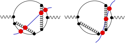
Virtual self-energy subgraphs, as in the right hand diagram in Fig. 3, require a special treatment. Consider a quark self-energy subdiagram with one adjoining virtual propagator and one adjoining cut propagator. This combination really represents a field strength renormalization for the quark field, and is interpreted as
| (10) |
In order to take the limit here while at the same time maintaining the cancellation of collinear divergences, we write
| (11) |
where . This expression is obtained by writing the left-hand side as a dispersive integral with the cut self-energy graph appearing as the discontinuity. When the virtual self-energy is written in this form, the limit is smooth and, in addition, the cancellation between the two cut diagrams in Fig. 3 in the collinear limit is manifest. It should be noted that the integral in Eq. (11) is ultraviolet divergent and requires renormalization, which can be performed with an ad hoc subtraction as described above.
One may expect that the representation of virtual propagator corrections in terms of the cut propagator will prove to be convenient in future modifications of the method described here. One may want to make modifications to the gluon propagator, in particular, in order to implement a running strong coupling and to insert models for the long distance propagation of gluons. In addition, one may want to modify propagators so that partons can enter the final state with so as to mesh an order perturbative calculation with a parton shower Monte Carlo program. In either case, the modified virtual gluon propagator should be related by a dispersive representation to the modified final state created by an outgoing gluon.
7 An example at order
I have argued that a completely numerical calculation of the observables considered here is possible in principle. The question now arises whether the principle can be put into operation in an actual computer program.
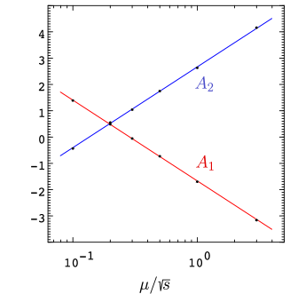
Consider first a simple example at one lower order in : the total cross section for at order . The cut diagrams are shown in Fig. 4.
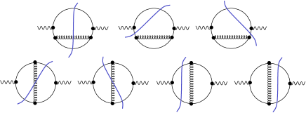
Let us define to be the sum of the top graphs in Fig. 4 and to be the sum of the bottom graphs, so that
| (12) |
Then a simple analytical calculation shows that
| (13) |
I have constructed a demonstration computer program to calculate and numerically along the lines described above. This example has UV renormalization, propagators to be treated dispersively, singularities to be avoided by deforming the contour, soft singularities that must cancel, and collinear singularities that must cancel. Thus it is not trivial from a numerical point of view. The results are shown in Fig. 5. Evidently, the method works.
8 An example at order
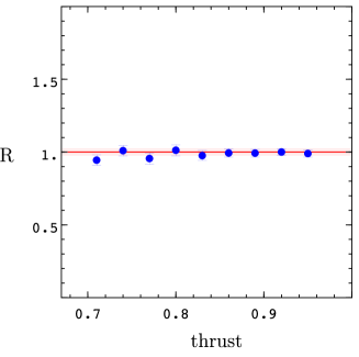
In order to further test the methods described here, I have constructed a demonstration computer program [6] to calculate three-jet-like observables for annihilation at order . I have used the program to calculate , the order contribution to the thrust distribution. More precisely, I have calculated the ratio of to , where where is a fit to the tabulated results for as given by Kunszt and Nason. [3] In the range , the function varies by about a factor of 30. The ratio should be 1. The results are reported in Fig. 6. Again, it appears that the numerical method of calculation works in a practical sense.
9 Outlook
I am working to test the code of the demonstration program. Indeed, between the time of the RADCOR98 conference and the time of this writing, I have found and corrected a small error in the program logic which resulted in an error in the calculation of about 1%. With this bug corrected, the results produced by the current version of the program are better than those shown in Fig. 6. After testing the code, I will have to document the code and publish a detailed description of the algorithms used.
With this code in hand, or with improved code from other authors, I anticipate attacks on more difficult problems than the problem discussed here. It remains to be seen for what problems the completely numerical method will prove to be more powerful than the analytical/numerical method that has served us so well up to now.
Acknowledgment
This work was supported by the U. S. Department of Energy.
References
References
- [1] D. E. Soper, Phys .Rev. Lett. 81, 2638 (1998).
- [2] R. K. Ellis, D. A. Ross, and A. E. Terrano, Nucl. Phys. B178, 421 (1981).
- [3] Z. Kunszt, P. Nason, G. Marchesini and B. R. Webber in Z Physics at LEP1, Vol. 1, edited by B. Altarelli, R. Kleiss ad C. Verzegnassi (CERN, Geneva, 1989), p. 373.
- [4] Z. Kunszt and D. E. Soper, Phys. Rev. D 46, 192 (1992).
- [5] G. Sterman, Phys. Rev. D 17, 2773, 2789 (1978).
- [6] The code used for Fig. 6, beowulf Version 0.7, is available at http://zebu.uoregon.edu/~soper/beowulf.html.