JLAB-THY-98-49

FACTORIZATION AND HIGH-ENERGY EFFECTIVE ACTION

IAN BALITSKY

Physics Department, Old Dominion University, Norfolk VA 23529

and

Theory Group, Jefferson Lab, Newport News VA 23606

e-mail: balitsky@jlab.org

Abstract

I demonstrate that the amplitude for high-energy scattering can be factorized as a convolution of the contributions due to fast and slow fields. The fast and slow fields interact by means of Wilson-line operators – infinite gauge factors ordered along the straight line. The resulting factorization formula gives a starting point for a new approach to the effective action for high-energy scattering in QCD.

PACS numbers: 12.38.Bx, 11.10.Jj, 11.55.Jy

I Introduction

In the leading logarithmic approximation, the high-energy scattering in perturbative QCD is determined by the BFKL pomeron [1]. It is well known that the power behavior of BFKL cross section violates the Froissart bound. The BFKL pomeron describes only the pre-asymptotic behavior at not very large energies and in order to find the true high-energy asymptotics in perturbative QCD we need to unitarize the BFKL pomeron. This is a difficult problem which has been in a need of a solution for more than 20 years. However, until recently, it was a common belief that at least at present energies (e.g. for small-x deep inelastic scattering in HERA) the corrections to BFKL pomeron are small so they can be neglected. Contrary to that expectations, recent calculation of the next-to-leading correction to the BFKL kernel [2] shows that this correction is very big. It is very likely that further corrections are also large which means that we must deal with the problem of the unitarization of the BFKL pomeron at present energies.

One of the most popular ideas on solving this problem is to reduce the QCD at high energies to some sort of two-dimensional effective theory which will be simpler than the original QCD, maybe even to the extent of exact solvability. Some attempts in this direction were made starting from the work [4] but the matter is an open issue for the time being. In this paper I will describe the new approach to the effective action which is based on the factorization in rapidity space for high-energy scattering.

The form of factorization is dictated by process kinematics (for a review, see [5]). A classical example is the factorization of the structure functions of deep inelastic scattering into coefficient functions and parton densities. In the case of deep inelastic scattering, there are two different scales of transverse momentum and it is therefore natural to factorize the amplitude in the product of contributions of hard and soft parts coming from the regions of small and large transverse momenta, respectively. On the contrary, in the case of high-energy (Regge-type) processes, all the transverse momenta are of the same order of magnitude, but colliding particles strongly differ in rapidity so it is natural to factorize in the rapidity space.

Factorization in rapidity space means that the high-energy scattering amplitude can be represented as a convolution of contributions due to “fast” and “slow” fields. To be precise, we choose a certain rapidity $\eta_{0}$ to be a “rapidity divide” and we call fields with $\eta>\eta_{0}$ fast and fields with $\eta<\eta_{0}$ slow where $\eta_{0}$ lies in the region between spectator rapidity $\eta_{A}$ and target rapidity $\eta_{B}$. (The interpretation of this fields as fast and slow is literally true only in the rest frame of the target but we will use this terminology for any frame).

To explain what we mean by the factorization in rapidity space let us recall the operator expansion for high-energy scattering [6] where the explicit integration over fast fields gives the coefficient functions for the Wilson-line operators representing the integrals over slow fields. For a 2$\Rightarrow$2 particle scattering in Regge limit $s\gg m^{2}$ (where $m$ is a common mass scale for all other momenta in the problem $t\sim p_{A}^{2}\sim(p^{\prime}_{A})^{2}\sim p_{B}^{2}\sim(p^{\prime}_{B})^{2}\sim m^{2}$) we have:

$$A(p_{A},p_{B}\Rightarrow p^{\prime}_{A},p^{\prime}_{B})=$$ (1)

$$\sum\int d^{2}x_{1}...d^{2}x_{n}C^{i_{1}...i_{n}}(x_{1},...x_{n})\langle p_{B}|{\rm Tr}\{U_{i_{1}}(x_{1})...U_{i_{n}}(x_{n})\}|p^{\prime}_{B}\rangle$$ (2)

(As usual, $s=(p_{A}+p_{B})^{2}$ and $t=(p_{A}-p^{\prime}_{A})^{2}$). Here $x_{i}~{}(i=1,2)$ are the transverse coordinates (orthogonal to both $p_{A}$ and $p_{B}$) and $U_{i}(x)=U^{\dagger}(x){i\over g}{\partial\over\partial x_{i}}U(x)$ where the Wilson-line operator $U(x)$ is the gauge link ordered along the infinite straight line corresponding to the “rapidity divide” $\eta_{0}$. Both coefficient functions and matrix elements in Eq. (1) depend on the $\eta_{0}$ but this dependence is canceled in the physical amplitude just as the scale $\mu$ (separating coefficient functions and matrix elements) disappears from the final results for structure functions in case of usual factorization. Typically, we have the factors $\sim(g^{2}\ln s/m^{2}-\eta_{0})$ coming from the “fast” integral and the factors $\sim g^{2}\eta_{0}$ coming from the “slow” integral so they combine in a usual log factor $g^{2}\ln s/m^{2}$. In the leading log approximation these factors sum up into the BFKL pomeron (for a review see ref. [7]).

Unlike usual factorization, the expansion (1) does not have the additional meaning of perturbative $vs$ nonperturbative separation – both the coefficient functions and the matrix elements have perturbative and non-perturbative parts. This happens due to the fact that the coupling constant in a scattering process is is determined by the scale of transverse momenta. When we perform the usual factorization in hard ($k_{\perp}>\mu$) and soft ($k_{\perp}<\mu$) momenta, we calculate the coefficient functions perturbatively (because $\alpha_{s}(k_{\perp}>\mu)$ is small) whereas the matrix elements are non-perturbative. Conversely, when we factorize the amplitude in rapidity, both fast and slow parts have contributions coming from the regions of large and small $k_{\perp}$. In this sense, coefficient functions and matrix elements enter the expansion (1) on equal footing. We could have integrated first over slow fields (having the rapidities close to that of $p_{B}$) and the expansion would have the form:

$$A(s,t)=\sum\int d^{2}x_{1}...d^{2}x_{n}D^{i_{1}...i_{n}}(x_{1},...x_{n})\langle p_{A}|{\rm Tr}\{U_{i_{1}}(x_{1})...U_{i_{n}}(x_{n})\}|p^{\prime}_{A}\rangle$$ (3)

In this case, the coefficient functions $D$ are the results of integration over slow fields ant the matrix elements of the $U$ operators contain only the large rapidities $\eta>\eta_{0}$. The symmetry between Eqs. (1) and (2) calls for a factorization formula which would have this symmetry between slow and fast fields in explicit form.

I will demonstrate that one can combine the operator expansions (1) and (3) in the following way:

$$A(s,t)=\sum{i^{n}\over n!}\int d^{2}x_{1}...d^{2}x_{n}$$ (4)

$$\langle p_{A}|U^{a_{1}i_{1}}(x_{1})...U^{a_{n}i_{n}}(x_{n})|p^{\prime}_{A}\rangle\langle p_{B}|U^{a_{1}}_{i_{1}}(x_{1})...U^{a_{n}}_{i_{n}}(x_{n})|p^{\prime}_{B}\rangle$$ (5)

where $U^{a}_{i}\equiv{\mathop{\rm Tr}}(\lambda^{a}U_{i})$ ($\lambda^{a}$ are the Gell-Mann matrices). It is possible to rewrite this factorization formula in a more visual form if we agree that operators $U$ act only on states $B$ and $B^{\prime}$ and introduce the notation $V_{i}$ for the same operator as $U_{i}$ only acting on the $A$ and $A^{\prime}$ states:

$$A(s,t)=\langle p_{A}|\langle p_{B}|\exp\left(i\!\int\!d^{2}xV^{ai}(x)U^{a}_{i}(x)\right)|p^{\prime}_{A}\rangle|p^{\prime}_{B}\rangle$$ (6)

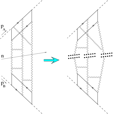
FIG. 1.: Structure of the factorization formula. Dashed, solid, and wavy lines denote photons, quarks, and gluons, respectively. Wilson-line operators are denoted by dotted lines and the vector $n$ gives the direction of the “rapidity divide” between fast and slow fields.

In a sense, this formula amounts to writing the coefficient functions in Eq. (1) (or Eq. (3)) as matrix elements of Wilson-line operators. Eq. (6) illustrated in Fig.1 is our main tool for factorizing in rapidity space.

In order to define an effective action for a given interval in rapidity $\eta_{0}>\eta>\eta^{\prime}_{0}$ we use the master formula (6) two times as illustrated in Fig. 2.

FIG. 2.: The effective action for the interval of rapidities $\eta_{0}>\eta>\eta^{\prime}_{0}$. The two vectors $n$ and $n^{\prime}$ correspond to “rapidity divides” $\eta_{0}$ and $\eta^{\prime}_{0}$ bordering our chosen region of rapidities

We obtain then

$$A(s,t)=\langle p_{A}|\langle p_{B}|e^{iS_{\rm eff}(V_{i},Y_{j})}|p^{\prime}_{A}\rangle|p^{\prime}_{B}\rangle$$ (7)

where the Wilson-line operators $Y_{i}(x_{\perp})$ have the same form as $U_{i}(x_{\perp})$ but aligned along the $n^{\prime}$ direction (and act only on $B$ and $B^{\prime}$ states, cf. eq. (6)). In this formula, the region of rapidities greater than $\eta_{0}$ is represented operators $V_{i}$ acting on the spectator $A$ and $A^{\prime}$ states, the region of rapidities lower than $\eta^{\prime}_{0}$ by the operators $Y_{i}$ acting on target $B$ and $B^{\prime}$ states, and the region $\eta_{0}>\eta>\eta^{\prime}_{0}$ is integrated out -all the information about it is contained in the effective action $S_{\rm eff}(V_{i},Y_{j})$. As we shall see below, this effective action is in general non-local (unlike the local interaction term $\int dx_{\perp}V_{i}(x_{\perp})U_{i}(x_{\perp})$ in the factorization formula (6)). Moreover, it contains the factors $g^{2}(\eta_{0}-\eta_{0}^{\prime})$ which are the usual high-energy logarithms $g^{2}\ln{s_{0}\over s^{\prime}_{0}}$ where the energies $s_{0}$ and $s^{\prime}_{0}$ correspond to rapidities $\eta_{0}$ and $\eta^{\prime}_{0}$. If we had a complete expression for $S_{\rm eff}(\eta_{0},\eta^{\prime}_{0})$ we could take $\eta_{0}=\eta_{A}$ (rapidity of the spectator particle) and $\eta^{\prime}_{0}=\eta_{B}$ (rapidity of the target particle), then all the logarithmic dependence on the energy would be included in the effective action and the resulting matrix elements of the operators $V_{i}$ between $A$ states and operators $Y$ between $B$ states will contain no logarithms (and may me calculated in the first order in perturbation theory for a suitable $A$ and $B$ particles such as virtual photons). Since multiple rescatterings are taken into account by $e^{iS_{\rm eff}}$ automatically the corresponding amplitude must be unitary. This program is probable not less difficult than the direct calculation of the many-pomeron exchanges in the perturbation theory but for the case of effective-action language we have some additional powerful methods such as semiclassical approach.

The paper is organized as follows. In Sect. 2 we remind the Wilson-line operator language for small-x physics. The factorization formula (6) is derived in Sect. 3 and in Sect. 4 we use it to define formally the high-energy effective action for a given interval in rapidity (Some of the results of this Sections were reported earlier in the letter [9]). A semiclassical approach to calculation of this effective action is discussed in Sect. 5 and Sect. 6 contains conclusions and outlook.

II Operator expansion for high-energy scattering

Let us now briefly remind how to obtain the operator expansion (1). For simplicity, consider the classical example of high-energy scattering of virtual photons with virtualities $\sim-~{}m^{2}$.

$$A(s,t)=-i{\mbox{$\langle 0|$}}T\{j(p_{A})j(p^{\prime}_{A})j(p_{B})j(p^{\prime}_{B})\}{\mbox{$|0\rangle$}}.$$ (8)

where $j(p)$ is the Fourier transform of electromagnetic current $j_{\mu}(x)$ multiplied by some suitable polarization $e^{\mu}(p)$. At high energies it is convenient to use the Sudakov decomposition:

$$p^{\mu}~{}=~{}\alpha_{p}p_{1}^{\mu}+\beta_{p}p_{2}^{\mu}+p_{\perp}^{\mu}$$ (9)

where $p_{1}^{\mu}$ and $p_{2}^{\mu}$ are the light-like vectors close to $p_{A}$ and $p_{B}$, respectively ($p_{A}^{\mu}=p_{1}^{\mu}-p_{2}^{\mu}p_{A}^{2}/s,~{}p_{B}^{\mu}=p_{2}^{\mu}-p_{1}^{\mu}p_{B}^{2}/s$). We want to integrate over the fields with $\alpha>\sigma$ where $\sigma$ is defined in such a way that the corresponding rapidity is $\eta_{0}$. (In explicit form $\eta_{0}=\ln{\sigma\over\tilde{\sigma}}$ where $\tilde{\sigma}\equiv{m^{2}\over s\sigma}$). The result of the integration will be given by Green functions of the fast particles in slow “external” fields [6] (see also ref. [10]). Since the fast particle moves along a straight-line classical trajectory the propagator is proportional to the straight-line ordered gauge factor $U$ [11]. For example, when $x_{+}>0,~{}y_{+}<0$ it has the form[6]:

$$G(x,y)=i\int\!dz\delta(z_{\ast})\frac{(\not\!\!x-\not\!\!z)\not\!\!p_{2}}{2\pi^{2}(x-z)^{4}}U(z_{\perp})\frac{\not\!\!z-\not\!\!y}{2\pi^{2}(z-y)^{4}}$$ (10)

We use the notations $z_{\bullet}\equiv z_{\mu}p_{1}^{\mu}$ and $z_{\ast}\equiv z_{\mu}p_{2}^{\mu}$ which are essentially identical to the light-front coordinates $z_{+}=z_{*}/\sqrt{s},~{}z_{-}=z_{\bullet}/\sqrt{s}$. The Wilson-line operator $U$ is defined as

$$U(x_{\perp})=[\infty p_{1}+x_{\perp},-\infty p_{1}+x_{\perp}]$$ (11)

where $[x,y]$ is the straight-line ordered gauge link suspended between the points $x$ and $y$:

$$[x,y]{\stackrel{{\scriptstyle\rm def}}{{\equiv}}}P\exp\left(ig\int_{0}^{1}du(x-y)^{\mu}A_{\mu}(ux+(1-u)y)\right)$$ (12)

The origin of Eq. (10) is more clear in the rest frame of the “A” photon (see Fig.2).

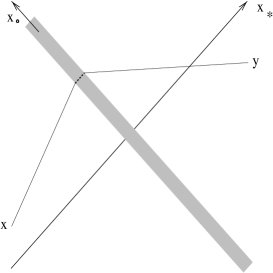
FIG. 3.: Quark propagator in a shock-wave background

Then the quark is slow and the external fields are approaching this quark at high speed. Due to the Lorentz contraction, these fields are squeezed in a shock wave located at $z_{*}=0$ (in a suitable gauge like the Feynman one). Therefore, the propagator (10) of the quark in this shock-wave background is a product of three factors which reflect (i) free propagation from $x$ to the shock wave (ii) instantaneous interaction with the shock wave which is described by the operator $U(z_{\perp})$ , and (iii) free propagation from the point of interaction $z$ to the final destination $y$.

The propagation of the quark-antiquark pair in the shock-wave background is described by the product of two propagators of Eq. (10) type which contain two Wilson-line factors $U(z)U^{\dagger}(z^{\prime})$ where $z^{\prime}$ is the point where the antiquark crosses the shock wave. If we substitute this quark-antiquark propagator in the original expression for the amplitude (8) we obtain[6]:

$$\int\!d^{4}xd^{4}ze^{ip_{A}\cdot x+iq\cdot z}\langle T\{j(x+z)j(z)\}\rangle_{A}\simeq$$ (13)

$$\int\frac{d^{2}p_{\perp}}{4\pi^{2}}I(p_{\perp},q_{\perp}){\mathop{\rm Tr}}\{U(p_{\perp})U^{\dagger}(q_{\perp}-p_{\perp})\}$$ (14)

where $U(p_{\perp})$ is the Fourier transform of $U(x_{\perp})$ and $I(p_{\perp},q_{\perp})$ is the so-called “impact factor” which is a function of $p_{\perp}^{2},p_{\perp}\!\cdot\!q_{\perp}$, and photon virtuality [12],[6]. Thus, we have reproduced the leading term in the expansion (1). (To recognize it, note that $U^{\dagger}(x_{\perp})U(y_{\perp})=P\exp\left\{-ig\int^{x}_{y}dz_{i}U_{i}(z_{\perp})\right\}$ where the precise form of the path between points $x_{\perp}$ and $y_{\perp}$ does not matter since this is actually a formula for the gauge link in a pure gauge field $U_{i}(z_{\perp})$). So, in the leading order in perturbation theory we have calculated the integral over fast fields explicitly and reduced the remaining integral over slow fields to the matrix element of the two-Wilson-line operator, see Fig. 4. It is worth noting that in the next order in perturbation theory we will get the contribution to the r.h.s of Eq. (14) proportional to four-Wilson-line operators, in the next to six-line operators and so on.

Note that formally we have obtained the operators $U$ ordered along the light-like lines. Matrix elements of such operators contain divergent longitudinal integrations which reflect the fact that light-like gauge factor corresponds to a quark moving with speed of light (i.e., with infinite energy). This divergency can be seen already at the one-loop level if one calculates the contribution to the matrix element of the two-Wilson-line operator $U(x_{\perp})U^{\dagger}(y_{\perp})$ between the ”virtual photon states” shown in Fig. 4.

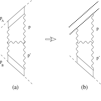
FIG. 4.: A typical Feynman diagram for the $\gamma^{*}\gamma^{*}$ scattering amplitude (a) and the corresponding two-Wilson-line operator (b)

The reason for this divergency is very simple. We have replaced the fast-quark propagator in the ”external field” (represented here by two gluons coming from the bottom part of the diagram) by the light-like Wilson line. In doing so we have assumed that these two gluons are slow, $\eta_{p}\ll\eta_{A}$. However, when we calculate the matrix element of the $U(x_{\perp})U^{\dagger}(y_{\perp})$ formally the integration over the rapidities of the gluon $\eta_{p}$ is unbounded so our divergency comes from the fast part of the external field which really does not belong there. Indeed, if the rapidity of the gluon $\eta_{p}$ is of the order of the rapidity of the quark this gluon is a fast one so it will contribute to the coefficient function (in front of the operator constructed from the slow fields) rather than to the matrix element of the operator.

This is very similar to the case of usual light-cone expansion for the deep inelastic scattering (DIS) at moderate x. In that case , we at first expand near the light cone (in inverse powers of $Q^{2}$). The result is that the amplitude of DIS is reduced to matrix elements of the light-cone operators which are known as parton densities in the nucleon. These matrix elements contain logarithmical divergence in transverse momenta for the same reason as above - when expanding around the light cone we assumed that there are no hard quarks and gluons inside the proton, but matrix elements of light-cone operators contain formally unbounded integrations over $k_{\perp}^{2}$. It is well known how to proceed in this case: we define the renormalized light-cone operators with the transverse momenta $k_{\perp}^{2}>\mu^{2}$ cut off and expand our T-product of electromagnetic currents in a set these renormalized light-cone operators rather than in a set of the original unrenormalized ones (see e.g. [8]). After that, the matrix elements of these operators (parton densities) contain factors $\ln{\mu^{2}\over m^{2}}$ and the corresponding coefficient functions contain $\ln{Q^{2}\over\mu^{2}}$. When we calculate the amplitude we add these factors together so the dependence on the factorization scale $\mu$ cancels and we get the usual DIS logarithmical factors $\ln{Q^{2}\over m^{2}}$.

Similarly, we need some regularization of the Wilson-line operator which cuts off the fast gluons. As demonstrated in [6], It can be done by changing the slope of the supporting line as demonstrated in [6]. If we wish the longitudinal integration stop at $\eta=\eta_{0}$, we should order our gauge factors $U$ along a line parallel to $n=\sigma p_{1}+\tilde{\sigma}p_{2}$, then the coefficient functions in front of Wilson-line operators (impact factors) will contain logarithms $\sim g^{2}\ln 1/\sigma$. Similarly to DIS, when we calculate the amplitude, we add the terms $\sim g^{2}\ln 1/\sigma$ coming from the coefficient functions (see Fig. 5b) to the terms $\sim g^{2}\ln{\sigma\over m^{2}/s}$ coming from matrix elements (see Fig. 5a) so that the dependence on the “rapidity divide” $\sigma$ cancels and we get the usual high-energy factors $g^{2}\ln{s\over m^{2}}$ which are responsible for BFKL pomeron.

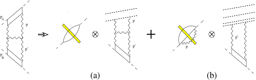
FIG. 5.: Decomposition into product of coefficient function and matrix element of the two-Wilson-line operator for a typical Feynman diagram. (Double Wilson line corresponds to fast-moving gluon)

III Factorization formula for high-energy scattering

In order to understand how this expansion can be generated by the factorization formula of Eq. (4) type we have to rederive the operator expansion in axial gauge $A_{\bullet}=0$ with an additional condition $\left.A_{*}\right|_{x_{*}=-\infty}=0$ (the existence of such a gauge was illustrated in [13] by an explicit construction). It is important to note that with with power accuracy (up to corrections $\sim\sigma$) our gauge condition may be replaced by $n^{\mu}A_{\mu}=0$. In this gauge the coefficient functions are given by Feynman diagrams in the external field

$$B_{i}(x)=U_{i}(x_{\perp})\Theta(x_{*}),~{}~{}~{}~{}~{}~{}~{}~{}~{}~{}~{}~{}~{}~{}~{}B_{\bullet}=B_{*}=0$$ (15)

which is a gauge rotation of our shock wave (it is easy to see that the only nonzero component of the field strength tensor $F_{\bullet i}(x)=U_{i}(x_{\perp})\delta(x_{*})$ corresponds to shock wave). The Green functions in external field (15) can be obtained from a generating functional with a source responsible for this external field. Normally, the source for given external field $\bar{{\cal A}}_{\mu}$ is just $J_{\nu}=\bar{D}^{\mu}\bar{F}_{\mu\nu}$ so in our case the only non-vanishing contribution is $J_{*}(B)=\bar{D}^{i}\bar{F}_{i*}$. However, we have a problem because the field which we try to create by this source does not decrease at infinity. To illustrate the problem, suppose that we use another light-like gauge ${\cal A}_{*}=0$ for a calculation of the propagators in the external field (15). In this case, the only would-be nonzero contribution to the source term in the functional integral $\bar{D}^{i}\bar{F}_{i_{\bullet}}{\cal A}_{*}$ vanishes, and it looks like we do not need a source at all to generate the field $B_{\mu}$! (This is of course wrong since $B_{\mu}$ is not a classical solution). What it really means is that the source in this case lies entirely at the infinity. Indeed, when we are trying to make an external field $\bar{{\cal A}}$ in the functional integral by the source $J_{\mu}$ we need to make a shift ${\cal A}_{\mu}\rightarrow{\cal A}_{\mu}+\bar{{\cal A}}_{\mu}$ in the functional integral

$$\int{\cal D}{\cal A}\exp\left\{iS({\cal A})-i\!\int\!d^{4}xJ^{a}_{\mu}(x){\cal A}^{a\mu}(x)\right\}$$ (16)

after which the linear term $\bar{D}^{\mu}\bar{F}_{\mu\nu}{\cal A}^{\nu}$ cancels with our source term $J_{\mu}{\cal A}^{\mu}$ and the terms quadratic in ${\cal A}$ make the Green functions in the external field $\bar{\cal A}$. (Note that the classical action $S(\bar{{\cal A}})$ for our external field $\bar{{\cal A}}=B$ (15) vanishes). However, in order to reduce the linear term $\int d^{4}x\bar{F}^{\mu\nu}\bar{D}_{\mu}{\cal A}_{\nu}$ in the functional integral to the form $\int d^{4}x\bar{D}^{\mu}\bar{F}_{\mu\nu}{\cal A}^{\nu}(x)$ we need to make an integration by parts, and if the external field does not decrease there will be additional surface terms at infinity. In our case we are trying to make the external field $\bar{{\cal A}}=B$ so the linear term which need to be canceled by the source is

$${2\over s}\int\!dx_{\bullet}dx_{*}d^{2}x_{\perp}\bar{F}_{i\bullet}\bar{D}_{*}{\cal A}^{i}=\left.\int\!dx_{*}d^{2}x_{\perp}\bar{F}_{i\bullet}{\cal A}^{i}\right|^{x_{\bullet}=\infty}_{x_{\bullet}=-\infty}$$ (17)

It comes entirely from the boundaries of integration. If we recall that in our case $\bar{F}_{\bullet i}(x)=U_{i}(x_{\perp})\delta(x_{*})$ we can finally rewrite the linear term as

$$\int\!d^{2}x_{\perp}U_{i}(x_{\perp})\{{\cal A}^{i}(-\infty p_{2}+x_{\perp})-{\cal A}^{i}(\infty p_{2}+x_{\perp})\}$$ (18)

The source term which we must add to the exponent in the functional integral to cancel the linear term after the shift is given by Eq. (18) with the minus sign. Thus, Feynman diagrams in the external field (15) in the light-like gauge ${\cal A}_{*}=0$ are generated by the functional integral

$$\!\int\!{\cal D}{\cal A}\exp\Big{\{}iS({\cal A})+i\!\int\!d^{2}x_{\perp}U^{ai}(x_{\perp})[{\cal A}^{a}_{i}(\infty p_{2}+x_{\perp})-{\cal A}^{ai}(-\infty p_{2}+x_{\perp})]\Big{\}}$$ (19)

In an arbitrary gauge the source term in the exponent in Eq. (19) can be rewritten in the form

$$2i\int d^{2}x_{\perp}{\mathop{\rm Tr}}\{U^{i}(x_{\perp})\int^{\infty}_{-\infty}dv[-\infty p_{2},vp_{2}]_{x_{\perp}}F_{*i}(vp_{2}+x_{\perp})[vp_{2},-\infty p_{2}]_{x_{\perp}}\}$$ (20)

(Hereafter we use the space-saving notation $[up_{2},vp_{2}]_{x_{\perp}}\equiv[up_{2}+x_{\perp},vp_{2}+x_{\perp}]$ and similar notation for gauge link ordered along $p_{1}$). Thus, we have found the generating functional for our Feynman diagrams in the external field (16).

It is instructive to see how the source (20) creates the field (15) in perturbation theory. To this end, we must calculate the field

$$\bar{\cal A}_{\mu}(x) = \!\int\!{\cal D}{\cal A}{\cal A}_{\mu}(x)\exp\Big{\{}iS({\cal A})+2i\!\int d^{2}x_{\perp}{\mathop{\rm Tr}}\{U^{i}(x_{\perp})$$ (21)

$$\int^{\infty}_{-\infty}dv[-\infty p_{2},vp_{2}]_{x_{\perp}}F_{*i}(vp_{2}+x_{\perp})[vp_{2},-\infty p_{2}]_{x_{\perp}}\}\Big{\}}$$ (22)

by expansion of both $S({\cal A})$ and gauge links in the source term (20) in powers of $g$ (see Fig. 6).

FIG. 6.: Perturbative diagrams for the classical field (15)

In the first order one gets

$$\bar{\cal A}^{(0)}_{\mu}(x)=\int^{\infty}_{-\infty}dv\int dz_{\perp}U^{ia}(z_{\perp})\langle{\cal A}_{\mu}(x)F^{a}_{*i}(vp_{2}+z_{\perp})\rangle$$ (23)

where $\langle{\cal O}\rangle\equiv\int\!{\cal D}{\cal A}e^{iS_{0}}{\cal O}$. Now we must choose a proper gauge for our calculation. We are trying to create a field (15) perturbatively and therefore the gauge for our perturbative calculation must be compatible with the form (15) — otherwise, we will end up with the gauge rotation of the field $B(x)$. (For example, in Feynman gauge we will get the field $\bar{\cal A}_{\mu}$ of the form of the shock wave $\bar{\cal A}_{i}=\bar{\cal A}_{\ast}=0,~{}\bar{\cal A}_{\bullet}\sim\delta(x_{\ast})$). It is convenient to choose the temporal gauge ${\cal A}_{0}=0$ with the boundary condition $\left.{\cal A}\right|_{t=-\infty}=0$ where

$${\cal A}_{\mu}(t,\vec{x})=\int^{t}_{-\infty}dt^{\prime}F_{0\mu}(t^{\prime},\vec{x})$$ (24)

In this gauge we obtain

$$\bar{\cal A}^{(0)}_{\mu}(x) = \int\!{dp\over(2\pi)^{3}}\left(g_{\mu\nu}-2{p_{\mu}(p_{1}+p_{2})_{\nu}+(\mu\leftrightarrow\nu)\over s(\alpha+\beta+i\epsilon)}+{4p_{\mu}p_{\nu}\over s^{2}(\alpha+\beta+i\epsilon)^{2}}\right)$$ (25)

$${1\over\alpha\beta s-p_{\perp}^{2}+i\epsilon}\int dz_{\perp}e^{i\alpha x_{\bullet}+i\beta x_{\ast}-i\vec{p}_{\perp}(\vec{x}-\vec{z})_{\perp}}p_{2\nu}\delta(\alpha{s\over 2})\partial_{i}U^{ia}(z_{\perp})$$ (26)

where $\delta(\alpha{s\over 2})$ comes from the $\int dve^{iv\alpha{s\over 2}}$. (Note that the form of the singularity ${1\over(p_{0}+i\epsilon)}$ which follops from Eq. (24) differs from conventional Mandelstam-Leibbrandt prescription $V.p.{1\over p_{0}}$). Recalling that in terms of Sudakov variables $dp={s\over 2}d\alpha d\beta dp_{\perp}$ one easily gets that $\bar{\cal A}^{(0)}_{\ast}=\bar{\cal A}^{(0)}_{\bullet}=0$ and

$$\bar{\cal A}^{(0)}_{i}(x) = \theta(x_{\ast})\int\!{dp\over(2\pi)^{2}}{1\over p_{\perp}^{2}}\int dz_{\perp}e^{-i\vec{p}_{\perp}(\vec{x}-\vec{z})_{\perp}}\partial_{i}\partial_{j}U^{ja}(z_{\perp})$$ (27)

which can be written down formally as

$$-\theta(x_{\ast}){1\over\partial_{\perp}^{2}}\partial_{i}\partial_{j}U^{j}(x_{\perp})=U_{i}(x_{\perp})\theta(x_{\ast})-\theta(x_{\ast}){1\over\partial_{\perp}^{2}}(\partial_{\perp}^{2}g_{ij}+\partial_{i}\partial_{j})U^{j}(x_{\perp})$$ (28)

(in our notations $\partial_{\perp}^{2}\equiv-\partial_{i}\partial^{i}$). Now, since $U_{i}(x)$ is a pure gauge field (with respect to transverse coordinates) we have $\partial_{i}U_{j}-\partial_{j}U_{i}=i[U_{i},U_{j}]$ so

$$\bar{\cal A}^{(0)}_{i}(x)=U_{i}(x_{\perp})\theta(x_{\ast})-\theta(x_{\ast})ig{\partial_{j}\over\partial_{\perp}^{2}}[U_{i},U_{j}])(x_{\perp})$$ (29)

Thus, we have reproduced the field (15) up to the correction of of $g$. We will demonstrate now that this $O(g)$ correction is canceled by the next-to-leading term in the expansion of the exponent of the source term in eq. (22). In the next-to-leading order one gets (see Fig. 6b):

$$\bar{\cal A}^{(1)}_{\mu}(x)=g\int\!dy\int\!dz_{\perp}dz^{\prime}_{\perp}U^{ja}(z_{\perp})U^{kb}(z^{\prime}_{\perp})$$ (30)

$$\langle{\cal A}_{\mu}(x)2{\rm Tr}\{\partial_{\alpha}{\cal A}_{\beta}(y)[{\cal A}_{\alpha}(y),{\cal A}_{\beta}(y)]\}\int\!dvF^{a}_{*j}(vp_{2}+z_{\perp})\int\!dv^{\prime}F^{b}_{*k}(vp_{2}+z^{\prime}_{\perp})\rangle$$ (31)

It is easy to see that $\bar{\cal A}^{(1)}_{\ast}=\bar{\cal A}^{(1)}_{\bullet}=0$ and

$$\bar{\cal A}^{(1)}_{i}(x)=$$ (32)

$$g\int\!dy\int{dp\over(2\pi)^{4}i}e^{-ip(x-y)}{1\over p^{2}}\left(\partial^{k}[{\cal A}^{(0)}_{i}(y),{\cal A}^{(0)}_{k}(y)]+[{\cal A}^{(0)k}(y),\partial_{i}{\cal A}^{(0)}_{k}(y)-(i\leftrightarrow k)]\right)$$ (33)

Since ${\cal A}^{(0)}_{k}$ is given by Eq. (29) this reduces to

$$\bar{\cal A}^{(1)}_{i}(x)=-g\theta(x_{\ast})\!\int\!dy_{\perp}{dp_{\perp}\over(2\pi)^{2}}{e^{-ip_{\perp}(x-y)_{\perp}}\over p_{\perp}^{2}}i\partial^{k}([U_{i}(y),U_{k}(y)])+O(g^{2})$$ (34)

which cancels the second term in Eq. (29). Thus, we obtain

$$\bar{\cal A}_{i}(x)=U_{i}(x_{\perp})\theta(x_{\ast})+O(g^{2})$$ (35)

Similarly, one can check that the contributions $\sim g^{2}$ coming the diagrams in Fig. 6c cancel the $g^{2}$ term in the Eq. (35) and so on leading finally to the expression $U_{i}(x_{\perp})\theta(x_{\ast})$ without any corrections.

We have found the generating functional for the diagrams in the external field (15) which give the coefficient functions in front of our Wilson-line operators $U_{i}$. Note that formally we obtained the source term with the gauge link ordered along the light-like line which is a potentially dangerous situation. Indeed, it it is easy to see that already the first loop diagram shown in Fig. 7 is divergent.

FIG. 7.: A typical loop diagram in the external field created by the Wilson-line source (20)

The reason is that the longitudinal integrals over $\alpha_{p}$ are unrestricted from below (if the Wilson line is light-like). However, this is not what we want for the coefficient functions because they should include only the integration over the region $\alpha_{p}>\sigma$ (the region $\alpha_{p}<\sigma$ belongs to matrix elements, see the discussion in Sect. 3). Therefore, we must impose somehow this condition $\alpha_{p}>\sigma$ in our Feynman diagrams created by the source (20). Fortunately, we already faced similar problem — how to impose a condition $\alpha_{p}<\sigma$ on the matrix elements of operators $U$ (see Fig. 4) and we have solved that problem by changing the slope of the supporting line. We demonstrated that in order to cut the integration over large $\alpha>\sigma$ from matrix elements of Wilson-line operators $U_{i}$ we need to change the slope of these Wilson-line operators to $n=\sigma p_{1}+\tilde{\sigma}p_{2}$. Similarly, if we want to cut the integration over small $\alpha_{p}<\sigma$ from the coefficient functions we need to order the gauge factors in Eq.(20) along (the same) vector $n=\sigma p_{1}+\tilde{\sigma}p_{2}$ .

Therefore, the final form of the generating functional for the Feynman diagrams (with $\alpha>\sigma$ cutoff) in the external field (16) is

$$\int\!{\cal D}{\cal A}{\cal D}\Psi{\rm exp}\left\{iS({\cal A},\Psi)+i\int d^{2}x_{\perp}U^{ai}(x_{\perp})V^{a}_{i}(x_{\perp})\right\}$$ (36)

where

$$V_{i}(x_{\perp})=$$ (37)

$$\int^{\infty}_{-\infty}dv[-\infty n,vn]_{x_{\perp}}n^{\mu}F_{\mu i}(vn+x_{\perp})[vn,-\infty n]_{x_{\perp}}$$ (38)

and $V^{a}_{i}\equiv{\rm Tr}(\lambda^{a}V_{i})$ as usual. For completeness, we have added integration over quark fields so $S({\cal A},\Psi)$ is the full QCD action.

Now we can assemble the different parts of the factorization formula (6). We have written down the generating functional integral for the diagrams with $\alpha>\sigma$ in the external fields with $\alpha<\sigma$ and what remains now is to write down the integral over these “external” fields. Since this integral is completely independent of (36) we will use a different notation ${\cal B}$ and $\chi$ for the $\alpha<\sigma$ fields. We have:

$$\int\!\!{\cal D}A{\cal D}\bar{\Psi}{\cal D}\Psi e^{iS(A,\Psi)}j(p_{A})j(p^{\prime}_{A})j(p_{B})j(p^{\prime}_{B})=$$ (39)

$$\int\!\!{\cal D}{\cal A}{\cal D}\bar{\psi}{\cal D}\psi e^{iS({\cal A},\psi)}j(p_{A})j(p^{\prime}_{A})\int\!\!{\cal D}{\cal B}{\cal D}\bar{\chi}{\cal D}\chi$$ (40)

$$j(p_{B})j(p^{\prime}_{B})e^{iS({\cal B},\chi)}\exp\Big{\{}i\!\int\!d^{2}x_{\perp}U^{ai}(x_{\perp})V^{a}_{i}(x_{\perp})\Big{\}}$$ (41)

The operator $U_{i}$ in an arbitrary gauge is given by the same formula (37) as operator $V_{i}$ with the only difference that the gauge links and $F_{{\bullet}i}$ are constructed from the fields ${\cal B}_{\mu}$. This is our factorization formula (6) in the functional integral representation.

The functional integrals over ${\cal A}$ fields give logarithms of the type $g^{2}\ln{1/\sigma}$ while the integrals over slow ${\cal B}$ fields give powers of $g^{2}\ln(\sigma s/m^{2})$. With logarithmic accuracy, they add up to $g^{2}\ln s/m^{2}$. However, there will be additional terms $\sim g^{2}$ due to mismatch coming from the region of integration near the dividing point $\alpha\sim\sigma$ where the details of the cutoff in the matrix elements of the operators $U$ and $V$ become important. Therefore, one should expect the corrections of order of $g^{2}$ to the effective action $\int dx_{\perp}U^{i}V_{i}$. Still, the fact that the fast quark moves along the straight line has nothing to do with perturbation theory (cf. ref. [14]); therefore it is natural to expect the non-perturbative generalization of the factorization formula (39) constructed from the same Wilson-line operators $U_{i}$ and $V_{i}$ (probably with some kind of non-local interactions between them).

IV Effective action for high-energy scattering

The factorization formula gives us a starting point for a new approach to the analysis of the high-energy effective action. Consider another rapidity $\eta^{\prime}_{0}$ in the region between $\eta_{0}$ and $\eta_{B}=\ln m^{2}/s$. If we use the factorization formula (39) once more, this time dividing between the rapidities greater and smaller than $\eta^{\prime}_{0}$, we get the expression for the amplitude (8) in the form :

$$iA(s,t) = \int\!\!{\cal D}Ae^{iS(A)}j(p_{A})j(p^{\prime}_{A})j(p_{B})j(p^{\prime}_{B})$$ (42)

$$= \int\!\!{\cal D}{\cal A}e^{iS({\cal A})}j(p_{A})j(p^{\prime}_{A})\int\!\!{\cal D}{\cal B}e^{iS({\cal B})}j(p_{B})j(p^{\prime}_{B})$$ (43)

$$\int\!{\cal D}{\cal C}e^{iS({\cal C})}e^{i\!\int\!d^{2}x_{\perp}V^{ai}(x_{\perp})U^{a}_{i}(x_{\perp})+i\!\int\!d^{2}x_{\perp}W^{ai}(x_{\perp})Y^{a}_{i}(x_{\perp})}$$ (44)

In this formula the operators $V_{i}$ (made from ${\cal A}$ fields) are given by Eq. (37), the operators $U_{i}$ are also given by Eq. (37) but constructed from the ${\cal C}$ fields instead, and the operators $W_{i}$ (made from ${\cal C}$ fields) and $Y_{i}$ (made from ${\cal B}$ fields) are aligned along the direction $n^{\prime}=\sigma^{\prime}p_{1}+\tilde{\sigma}^{\prime}p_{2}$ corresponding to the rapidity $\eta^{\prime}$ (as usual, $\ln\sigma^{\prime}/\tilde{\sigma}^{\prime}=\eta^{\prime}$ where $\tilde{\sigma}^{\prime}=m^{2}/s\sigma^{\prime}$):

$$U_{i}({\cal C})_{x_{\perp}}=\int^{\infty}_{-\infty}dv[-\infty n,vn]_{x_{\perp}}n^{\mu}F_{\mu i}(vn+x_{\perp})[vn,-\infty n]_{x_{\perp}}$$ (45)

$$W_{i}({\cal C})_{x_{\perp}}=\int^{\infty}_{-\infty}dv[-\infty n^{\prime},vn^{\prime}]_{x_{\perp}}n^{{}^{\prime}\mu}F_{\mu i}(vn^{\prime}+x_{\perp})[vn^{\prime},-\infty n^{\prime}]_{x_{\perp}}$$ (46)

$$Y_{i}({\cal B})_{x_{\perp}}=\int^{\infty}_{-\infty}dv[-\infty n^{\prime},vn^{\prime}]_{x_{\perp}}n^{{}^{\prime}\mu}F_{\mu i}(vn^{\prime}+x_{\perp})[vn^{\prime},-\infty n^{\prime}]_{x_{\perp}}$$ (47)

Thus, we have factorized the functional integral over “old” ${\cal B}$ fields into the product of two integrals over ${\cal C}$ and “new” ${\cal B}$ fields.

Now, let us integrate over the ${\cal C}$ fields and write down the result in terms of an effective action. Formally, one obtains:

$$iA(s,t)=\int\!\!{\cal D}{\cal A}e^{iS({\cal A})}j(p_{A})j(p^{\prime}_{A})\int\!\!{\cal D}{\cal B}e^{iS({\cal B})}j(p_{B})j(p^{\prime}_{B})e^{iS_{\rm eff}(V_{i},Y_{i};{\sigma\over\sigma^{\prime}})}$$ (48)

where $S_{\rm eff}$ for the rapidity interval between $\eta$ and $\eta^{\prime}$ is defined as

$$e^{iS_{\rm eff}(V_{i},Y_{i};{\sigma\over\sigma^{\prime}})}=\int\!{\cal D}{\cal C}e^{iS({\cal C})}e^{i\!\int\!d^{2}x_{\perp}V^{ai}(x_{\perp})U^{a}_{i}(x_{\perp})+i\!\int\!d^{2}x_{\perp}W^{ai}(x_{\perp})Y^{a}_{i}(x_{\perp})}$$ (49)

This formula gives a rigorous definition for the effective action for a given interval in rapidity (cf. ref. [7]).

Next step would be to perform explicitly the integrations over the longitudinal momenta in the r.h.s. of Eq. (49) and obtain the answer for the integration over our rapidity region (from $\eta$ to $\eta^{\prime}$) in terms of two-dimensional theory in the transverse coordinate space which hopefully would give us the unitarization of the BFKL pomeron. At present, it is not known how to do this. One can obtain, however, a first few terms in the expansion of effective action in powers of $V_{i}$ and $Y_{i}$. The easiest way to do this is to expand gauge factors $U_{i}$ and $W_{i}$ in r.h.s. of Eq. (49) in powers of ${\cal C}$ fields and calculate the relevant perturbative diagrams (see Fig. 8).

FIG. 8.: Lowest order terms in the perturbative expansion of the effective action.

The first few terms in the effective action at the one-log level

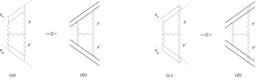
FIG. 9.: Counting of loops for Feynman diagrams (a),(c) and the corresponding Wilson-line operators (b),(d)

have the form [4],[17]:

$$S_{\rm eff}=\int d^{2}xV^{ai}(x)Y^{a}_{i}(x)-$$ (50)

$${g^{2}\over 64\pi^{3}}\ln{\sigma\over\sigma^{\prime}}\Big{(}N_{c}\int d^{2}xd^{2}yV^{a}_{i,i}(x)\ln^{2}(x-y)^{2}Y^{a}_{j,j}(y)+{f_{abc}f_{mnc}\over 4\pi^{2}}\!\int\!d^{2}xd^{2}yd^{2}x^{\prime}d^{2}y^{\prime}d^{2}z$$ (51)

$$V^{a}_{i,i}(x)V^{m}_{j,j}(y)Y^{b}_{k,k}(x^{\prime})Y^{n}_{l,l}(y^{\prime})\ln{(x-z)^{2}\over(x-x^{\prime})^{2}}\ln{(y-z)^{2}\over(y-y^{\prime})^{2}}\left({\partial\over\partial z_{i}}\right)^{2}\ln{(x^{\prime}-z)^{2}\over(x-x^{\prime})^{2}}\ln{(y^{\prime}-z)^{2}\over(y-y^{\prime})^{2}}\Big{)}+...$$ (52)

where we we use the notation $V^{a}_{i,j}(x)\equiv{\partial\over\partial x_{j}}V^{a}_{i}(x)$ etc. The first term (see Fig. 8a) looks like the corresponding term in the factorization formula (39) – only the directions of the supporting lines are now strongly different . The second term shown in Fig. 8c is the first-order expression for the reggeization of the gluon[1] and the third term (see Fig. 8d) is the two-reggeon Lipatov’s Hamiltonian[18] responsible for BFKL logarithms.

Let us discuss subsequent terms in the perturbative expansion (50). There can be two types of the logarithmical contributions. First is the ”true” loop contribution coming from the diagrams of the Fig.10a type. This diagram is an iteration of the Lipatov’s Hamiltonian. However, in the same $(\ln{\sigma\over\sigma^{\prime}})^{2}$ order there is another contribution coming from the diagram shown in Fig. 10b.

FIG. 10.: Typical perturbative diagrams in the next $\left(\ln{\sigma\over\sigma^{\prime}}\right)^{2}$ order.

To treat them separately, we can consider the case when $g\ll 1$ but the sources are strong ($\sim{1\over g}$) so $gY_{i}\sim gU_{i}\sim 1$. In this case, the diagram in Fig.10a has the order $g^{4}Y_{i}^{2}V_{i}^{2}\left(\ln{\sigma\over\sigma^{\prime}}\right)^{2}\sim\left(\ln{\sigma\over\sigma^{\prime}}\right)^{2}$ while the ”tree” Fig.8b diagram is $\sim g^{4}Y_{i}^{3}V_{i}^{3}\left(\ln{\sigma\over\sigma^{\prime}}\right)^{2}\sim{1\over g^{2}}\left(\ln{\sigma\over\sigma^{\prime}}\right)^{2}$. So, in this approximation the tree diagrams are the most important and should be summed up in the first place. As usual, the best way to sum the tree diagrams is given by the semiclassical method which will be discussed in next Section.

However, if we would like to get the result on the one-log level it can be obtained using the evolution equations for the Wilson-line operators [6]. Note that at this level we have only the diagrams of the Fig.11 type. These diagrams describe the situation when one of the sources is weak and another is still strong (see also refs. [20], [16]). For example, if the source $V_{i}$ is weak (and hence $gV_{i}$ is a valid small parameter) but the source $Y_{i}$ is not weak (so that $gV_{i}\sim 1$ is not a small parameter) one must take into account the diagrams shown in Fig. 11a and b.

FIG. 11.: Perturbative diagrams for the effective action in the case of one weak source and one strong one.

The multiple rescatterings in Fig. 11a,b describe the motion of the gluon emitted by the weak source $V_{i}$ in the strong external field $A_{i}=Y_{i}\theta(x_{\ast})$ created by the source $Y_{i}$. These diagrams were calculated in ref. [6]. For example, the result of the calculation of the diagram in Fig. 11a presented in a form of the evolution of the Wilson-line operators $U_{i}$ reads

$$U^{a}_{i}(x_{\perp})\rightarrow Y^{a}_{i}(x_{\perp})-$$ (53)

$${g^{2}\over 8\pi^{3}}\ln{\sigma\over\sigma^{\prime}}\int dy_{\perp}{1\over(x-y)_{\perp}^{2}}\Big{(}f^{abc}\big{(}Y^{\dagger}_{x}\partial_{i}Y_{y}\big{)}^{bc}+N_{c}U^{a}_{i}(x_{\perp})\Big{)}+...$$ (54)

where dots stand for the terms with extra $g^{2}\ln{\sigma\over\sigma^{\prime}}$ factors. This evolution equation means that if we integrate over the rapidities $\eta_{0}>\eta>\eta^{\prime}_{0}$ in the matrix elements of the operator $U_{i}$ we will get the expression (54) constructed from the operators $Y_{i}$ with rapidities up to $\eta^{\prime}_{0}$ times factors proportional to $g^{2}(\eta_{0}-\eta^{\prime}_{0})\equiv g^{2}\ln{\sigma\over\sigma^{\prime}}$. Therefore, the corresponding contribution to the effective action at the one-log level takes the form

$$\int dx_{\perp}V^{a}_{i}(x_{\perp})U^{ai}(x_{\perp})\rightarrow\int dx_{\perp}V^{a}_{i}(x_{\perp})Y^{ai}(x_{\perp})-$$ (55)

$${g^{2}\over 8\pi^{3}}\ln{\sigma\over\sigma^{\prime}}\int\!dx_{\perp}dy_{\perp}{1\over(x-y)_{\perp}^{2}}\Big{(}i\big{(}V^{i}(x_{\perp})Y^{\dagger}_{x}\partial_{i}Y_{y}\big{)}^{aa}-N_{c}V^{ai}(x_{\perp})U^{a}_{i}(x_{\perp})\Big{)}$$ (56)

where the first term is the lowest-order effective action ($\equiv$ the first term in eq. (50)) and the second term contains new information. To check this second term, we may expand it in powers of the source $Y_{i}$ and it is easy to see that the first nontrivial term in this expansion coincides with the gluon-reggeization term in eq. (50).

Apart from the (55) term, there is another contribution to the one-loop evolution equations coming from the diagrams in Fig. (11b) [6]:

$$U_{i}^{a}(x_{\perp})U_{j}^{b}(y_{\perp})\rightarrow$$ (57)

$$-{g^{2}\over 4\pi^{3}}\ln{\sigma\over\sigma^{\prime}}\Big{(}\nabla^{x}_{i}\Big{[}\int dz_{\perp}{(x-z)_{\perp}\cdot(y-z)_{\perp}\over(x-z)^{2}_{\perp}(y-z)^{2}_{\perp}}(Y^{\dagger}_{x}Y_{y}+1-Y^{\dagger}_{x}Y_{z}-Y^{\dagger}_{z}Y_{y})\Big{]}\stackrel{{\scriptstyle\leftarrow}}{{\nabla}}^{y}_{j}\Big{)}^{ab}$$ (58)

where

$$\nabla^{x}_{i}{\cal O}(x_{\perp}) \equiv {\partial\over\partial x^{i}}{\cal O}(x_{\perp})-iU_{i}(x_{\perp}){\cal O}(x_{\perp})$$ (59)

$${\cal O}(y_{\perp})\stackrel{{\scriptstyle\leftarrow}}{{\nabla}}^{y}_{i} \equiv -{\partial\over\partial y^{i}}{\cal O}(y_{\perp})-i{\cal O}(y_{\perp})U_{i}(y_{\perp})$$ (60)

are the “covariant derivatives” (in the adjoint representation). The corresponding term in effective action has the form

$${ig^{2}\over 8\pi^{3}}\ln{\sigma\over\sigma^{\prime}}\int dx_{\perp}dy_{\perp}\left(\nabla^{x}_{i}V^{a}_{i}\right)(x_{\perp})\int dz_{\perp}{(x-z)_{\perp}\cdot(y-z)_{\perp}\over(x-z)^{2}_{\perp}(y-z)^{2}_{\perp}}$$ (61)

$$\big{(}Y^{\dagger}_{x}Y_{y}+1-Y^{\dagger}_{x}Y_{z}-Y^{\dagger}_{z}Y_{y}\big{)}^{ab}\left(\nabla^{y}_{j}V^{b}_{j}\right)(y_{\perp})$$ (62)

The final form of the one-log effective action for this case is the sum of the expressions (55) and (62):

$$S^{(I)}_{\rm eff}(V_{i},Y_{j})=\int d^{2}xV^{ai}(x)Y^{a}_{i}(x)-$$ (63)

$${g^{2}\over 8\pi^{3}}\ln{\sigma\over\sigma^{\prime}}\int\!dx_{\perp}dy_{\perp}{1\over(x-y)_{\perp}^{2}}\Big{(}i\big{(}V^{i}(x_{\perp})Y^{\dagger}_{x}\partial_{i}Y_{y}\big{)}^{aa}-N_{c}V^{ai}(x_{\perp})U^{a}_{i}(x_{\perp})\Big{)}$$ (64)

$$+{ig^{2}\over 8\pi^{3}}\ln{\sigma\over\sigma^{\prime}}\int dx_{\perp}dy_{\perp}\nabla^{x}_{i}V^{ai}(x_{\perp})\int dz_{\perp}{(x-z)_{\perp}\cdot(y-z)_{\perp}\over(x-z)^{2}_{\perp}(y-z)^{2}_{\perp}}$$ (65)

$$\big{(}Y^{\dagger}_{x}Y_{y}+1-Y^{\dagger}_{x}Y_{z}-Y^{\dagger}_{z}Y_{y}\big{)}^{ab}\nabla^{y}_{j}V^{bj}(y_{\perp})$$ (66)

where $V_{i}$ is a weak source and $Y_{i}$ is a strong one. It is clear that if the source $V_{i}$ is strong and $Y_{i}$ is weak as shown in Fig. 10c,d diagrams the effective action $S^{(II)}_{\rm eff}(V_{i},Y_{j})$ will have the similar form with the replacement $V\leftrightarrow Y$.

As we mentioned above, the diagrams in Fig.10 and Fig. 11 complete the list of diagrams which contribute to the effective action at the one-log level (even if both sources are strong). It means that the one-log answer in general case can be guessed by comparison of the answers for $S^{(I)}_{\rm eff}(V_{i},Y_{j})$ and $S^{(II)}_{\rm eff}(V_{i},Y_{j})$ (the simple sum is not enough since some of the contributions will be double-counted). Instead of doing that, we will obtain the one-log result for two strong sources using the semiclassical method and check that it agrees with (63).

V Effective action and collision of two shock waves

The functional integral (49) which defines the effective action is the usual QCD functional integral with two sources corresponding to the two colliding shock waves. Instead of calculation of perturbative diagrams (as it was done in previous section) one can use the semiclassical approach. This approach is relevant when the coupling constant is relatively small but the characteristic fields are large (in other words, when $g^{2}\ll 1$ but $gV_{i}\sim gY_{i}\sim 1$). In this case one can calculate the functional integral (49) by expansion around the new stationary point corresponding to the classical wave created by the collision of the shock waves.

With leading log accuracy, we can replace the vector $n$ by $p_{1}$ and the vector $n^{\prime}$ by $p_{2}$. Then the functional integral (49) takes the form:

$$e^{iS_{\rm eff}(V_{i},Y_{i};{\sigma\over\sigma^{\prime}})}=\int\!{\cal D}Ae^{iS_{QCD}(A)}e^{i\!\int\!d^{2}x_{\perp}V^{ai}(x_{\perp})U^{a}_{i}(x_{\perp})+i\!\int\!d^{2}x_{\perp}W^{ai}Y^{a}_{i}(x_{\perp})}$$ (67)

where now

$$U^{a}_{i}(x_{\perp})=\int^{\infty}_{-\infty}dv\hat{F}_{\bullet i}(vp_{1}+x_{\perp}),~{}~{}~{}~{}~{}~{}~{}W^{a}_{i}=\int^{\infty}_{-\infty}dv\tilde{F}_{\ast i}(vp_{2}+x_{\perp})$$ (68)

Hereafter we use the notations

$$\hat{\cal O}(x) = [-\infty p_{1}+x,x]{\cal O}(x)[x,-\infty p_{1}+x]$$ (69)

$$\tilde{\cal O}(x) = [-\infty p_{2}+x,x]{\cal O}(x)[x,-\infty p_{2}+x]$$ (70)

Note that we changed the name for the gluon fields in the integrand from ${\cal C}$ back to $A$.

As usual, the classical equation for the saddle point $\bar{A}$ in the functional integral (67) is

$$\left.{\delta\over\delta A}\left(S_{QCD}+\!\int\!d^{2}x_{\perp}V^{ai}(x_{\perp})U^{a}_{i}(x_{\perp})+\!\int\!d^{2}x_{\perp}W^{ai}Y^{a}_{i}(x_{\perp}\right)\right|_{A=\bar{A}}=0$$ (71)

To write down them explicitly we need the first variational derivatives of the source terms with respect to gauge field. We have:

$$\delta U_{i}=\delta\hat{A}_{i}(\infty p_{1}+x_{\perp})-\delta{A}_{i}(-\infty p_{1}+x_{\perp})-\int^{\infty}_{-\infty}du\hat{\nabla}_{i}\delta\hat{A}_{i}(up_{1}+x_{\perp})$$ (72)

$$\delta W_{i}=\delta\tilde{A}_{i}(\infty p_{2}+x_{\perp})-\delta{A}_{i}(-\infty p_{2}+x_{\perp})-\int^{\infty}_{-\infty}du\tilde{\nabla}_{i}\delta\tilde{A}_{i}(up_{2}+x_{\perp})$$ (73)

where

$$\hat{\nabla}_{i}{\cal O}(x) \equiv \partial_{i}{\cal O}(x)-i[U_{i}(x_{\perp})+A_{i}(-\infty p_{1}+x_{\perp}),{\cal O}(x)]$$ (74)

$$\tilde{\nabla}_{i}{\cal O}(x) \equiv \partial_{i}{\cal O}(x)-i[W_{i}(x_{\perp})+A_{i}(-\infty p_{2}+x_{\perp}),{\cal O}(x)]$$ (75)

Therefore the explicit form of the classical equations (71) for the wave created by the collision is:

$$D^{\mu}F_{\mu i}=0$$ (76)

$$D^{\mu}F_{\ast\mu}=\delta({2\over s}x_{\bullet})[{2\over s}x_{\ast}p_{1},-\infty p_{1}]_{x_{\perp}}\hat{\nabla}_{i}V^{i}(x_{\perp})[-\infty p_{1},{2\over s}x_{\ast}p_{1}]_{x_{\perp}}$$ (77)

$$D^{\mu}F_{\bullet\mu}=\delta({2\over s}x_{\ast})[{2\over s}x_{\bullet}p_{2},-\infty p_{2}]_{x_{\perp}}\tilde{\nabla}_{i}Y^{i}(x_{\perp})[-\infty p_{2},{2\over s}x_{\bullet}p_{2}]_{x_{\perp}}$$ (78)

Also, as explained in Sect. 3, since our fields do not decrease at infinity there may be extra surface linear terms (cf. Eq. (17)) coming from the contributions proportional to $\delta A(\pm\infty)$ in the r.h.s. of eq. (73). The requirement of absence of such terms gives four additional equations

$$\left.F_{\bullet i}\right|_{x_{\bullet}=\infty} = \delta(2x_{\ast}/s)Y_{i}(x_{\perp}),~{}~{}~{}~{}~{}~{}~{}\left.F_{\ast i}\right|_{x_{\ast}=-\infty}=\delta(2x_{\bullet}/s)V_{i}(x_{\perp}),$$ (79)

$$\left.F_{\bullet i}\right|_{x_{\bullet}=\infty} = \delta(2x_{\ast}/s)[\infty p_{2},-\infty p_{2}]_{x_{\perp}}Y_{i}(x_{\perp})[-\infty p_{2},\infty p_{2}]_{x_{\perp}}$$ (80)

$$\left.F_{\ast i}\right|_{x_{\ast}=\infty} = \delta(2x_{\bullet}/s)[\infty p_{1},-\infty p_{1}]_{x_{\perp}}V_{i}(x_{\perp})[-\infty p_{1},\infty p_{1}]_{x_{\perp}}$$ (81)

The two sets of equations (76) and (79) define the classical field created by the collision of two shock waves .

Unfortunately, it is not clear how to solve these equations. One can start with the trial field which is a simple superposition of the two shock waves (15)

$$A^{(0)}_{\ast}=A^{(0)}_{\bullet}=0,~{}~{}~{}~{}A^{(0)}_{i}=\Theta(x_{\bullet})V_{i}+\Theta(x_{\ast})Y_{i}$$ (82)

and improve it by taking into account the interaction between the shock waves order by order[15]. The parameter of this expansion is the commutator $g^{2}[Y_{i},V_{k}]$. Moreover, it can be demonstrated that each extra commutator brings a factor $\ln{\sigma\over\sigma^{\prime}}$ and therefore this approach is a sort of leading logarithmic approximation. In the lowest nontrivial order one gets:

$$A^{(1)}_{i} = -{g\over 4\pi^{2}}\int dz_{\perp}([Y_{i}(z_{\perp}),V_{k}(z_{\perp})]-i\leftrightarrow k){(x-z)^{k}\over(x-z)_{\perp}^{2}}\ln\left(1-{(x-z)_{\perp}^{2}\over x_{\parallel}^{2}+i\epsilon}\right)$$ (83)

$$A^{(1)}_{\bullet} = {gs\over 16\pi^{2}}\int dz_{\perp}{1\over x_{\ast}+i\epsilon}\ln(-x_{\parallel}^{2}+(x-z)_{\perp}^{2}+i\epsilon)[Y_{k}(z_{\perp}),V^{k}(z_{\perp})]$$ (84)

$$A^{(1)}_{\ast} = -{gs\over 16\pi^{2}}\int dz_{\perp}{1\over x_{\bullet}+i\epsilon}\ln(-x_{\parallel}^{2}+(x-z)_{\perp}^{2}+i\epsilon)[Y_{k}(z_{\perp}),V^{k}(z_{\perp})]$$ (85)

where $x_{\parallel}^{2}\equiv{4\over s}x_{\ast}x_{\bullet}$ is a longitudinal part of $x^{2}$. These fields are obtained in the background-Feynman gauge. The corresponding expressions for field strength have the form:

$$F^{(1)}_{\bullet\ast} = {gs\over 4\pi^{2}}\int dz_{\perp}{1\over-x_{\parallel}^{2}+(x-z)_{\perp}^{2}+i\epsilon}[Y_{k},V^{k}]$$ (86)

$$F^{(1)}_{ik} = {g\over 2\pi^{2}}\int dz_{\perp}{1\over-x_{\parallel}^{2}+(x-z)_{\perp}^{2}+i\epsilon}([Y_{i},V_{k}]-[Y_{k},V_{i}])$$ (87)

$$F^{(1)}_{\bullet i} = {gs\over 8\pi^{2}}\!\int\!dz_{\perp}{(x-z)^{k}\over-x_{\parallel}^{2}+(x-z)_{\perp}^{2}+i\epsilon}\left({g_{ik}[Y_{j},V^{j}]\over x_{\ast}-i\epsilon}+{[Y_{i},V_{k}]-[Y_{k},V_{i}]\over x_{\ast}+i\epsilon}\right)$$ (88)

$$F^{(1)}_{\ast i} = -{gs\over 8\pi^{2}}\!\int\!dz_{\perp}{(x-z)^{k}\over-x_{\parallel}^{2}+(x-z)_{\perp}^{2}+i\epsilon}\left({g_{ik}[Y_{j},V^{j}]\over x_{\bullet}-i\epsilon}-{[Y_{i},V_{k}]-[Y_{k},V_{i}]\over x_{\bullet}+i\epsilon}\right)$$ (89)

In terms of usual Feynman diagrams (when we expand in powers of source just like in previous Section) these expressions come from the diagrams shown in Fig. 12.

FIG. 12.: Perturbative Feynman diagrams for the field strength (86)

When we sum up the three contributions from the diagrams in Fig. 12a,b, and c the three-gluon vertex in Fig. 12a is replaced by the effective Lipatov’s vertex and we get (86) up to the terms ${1\over\partial^{2}}\partial_{i}\partial_{k}Y^{k}$ and ${1\over\partial^{2}}\partial_{j}\partial_{k}V^{k}$ standing in place of $Y_{i}$ and $V_{j}$. However, as we have discussed in Sect. 3, the difference $Y_{i}-{1\over\partial^{2}}\partial_{i}\partial_{k}Y^{k}=g{\partial_{k}\over\partial^{2}}[Y_{i},Y_{k}]$ (which has an additional power of g) will be canceled by the next-order perturbative diagrams of the Fig. 12d type.

Let us now find the effective action. In the trivial order the only non-zero field strength components are $F^{(0)}_{\bullet i}=\delta({2\over s}x_{\ast})Y_{i}(x_{\perp})$ and $F^{(0)}_{\ast i}=\delta({2\over s}x_{\bullet})V_{i}(x_{\perp})$ so we get the familiar expression $S^{(0)}=\int d^{2}x_{\perp}V^{ai}Y^{a}_{i}$. In the next order one has

$$S^{(1)}=\int d^{4}x\left(-{2\over s}F_{\ast}^{(1)ai}F^{(1)a}_{\bullet i}-{1\over 4}F^{(1)a}_{ik}F^{(1)aik}+{2\over s^{2}}F^{(1)a}_{\ast\bullet}F^{(1)a}_{\ast\bullet}\right)+2\!\int\!d^{2}x_{\perp}$$ (90)

$$\int\!du\Big{(}{\rm Tr}V^{i}\left([-\infty p_{1},up_{1}]_{x_{\perp}}F_{\bullet i}(up_{1}+x_{\perp})[up_{1}+x_{\perp},-\infty p_{1}]_{x_{\perp}}\right)^{(1)}+$$ (91)

$${\rm Tr}Y^{i}\left(-\infty p_{2},up_{2}]_{x_{\perp}}F_{\ast i}(up_{2}+x_{\perp})[up_{2},\infty p_{2}]_{x_{\perp}}\right)^{(1)}\Big{)}$$ (92)

We have seen above that the effective action contains $\ln{\sigma\over\sigma^{\prime}}$ (see Eq. (50)). With logarithmic accuracy, the r.h.s of Eq. (92) reduces to

$$S^{(1)} = -{2\over s}\int d^{4}xF^{(1)ai}_{\ast}(x)F_{\bullet i}^{(1)a}(x)$$ (93)

$$+ \int d^{2}x_{\perp}2{\rm Tr}[Y^{i},V_{i}]\left([x_{\perp},-\infty p_{2}+x_{\perp}]^{(1)}-[x_{\perp},-\infty p_{1}+x_{\perp}]^{(1)}\right)$$ (94)

The first term contains the integral over $d^{4}x={2\over s}dx_{\bullet}dx_{\ast}d^{2}x_{\perp}$. In order to separate the longitudinal divergencies from the infrared divergencies in the transverse space we will work in the $d=2+2\epsilon$ transverse dimensions. It is convenient to perform at first the integral over $x_{\ast}$ which is determined by a residue in the point $x_{\ast}=0$. The integration over remaining light-cone variable $x_{\bullet}$ factorizes then in the form $\int_{0}^{\infty}dx_{\bullet}/x_{\bullet}$ or $\int_{-\infty}^{0}dx_{\bullet}/x_{\bullet}$. This integral reflects our usual longitudinal logarithmic divergencies which arise from the replacement of vectors $n$ and $n^{\prime}$ in (49) by the light-like vectors $p_{1}$ and $p_{2}$. In the momentum space this logarithmical divergency has the form $\int d\alpha/\alpha$. It is clear that when $\alpha$ is close to $\sigma$ (or $\sigma^{\prime}$) we can no longer approximate $n$ by $p_{1}$ (or $n^{\prime}$ by $p_{2}$). Therefore, in the leading log approximation this divergency should be replaced by $\ln{\sigma\over\sigma^{\prime}}$:

$$\int_{0}^{\infty}dx_{\bullet}{1\over x_{\bullet}}=\int_{0}^{\infty}d\alpha{1\over\alpha}\rightarrow\int_{\sigma}^{\sigma^{\prime}}d\alpha{1\over\alpha}~{}=~{}\ln{\sigma\over\sigma^{\prime}}$$ (95)

The (first-order) gauge links in the second term in r.h.s. of Eq. (94) have the logarithmic divergence of the same origin:

$$[x_{\perp},-\infty p_{1}+x_{\perp}]^{(1)}=-{i\over 8\pi^{2}}\int^{0}_{-\infty}\!{dx_{\ast}\over x_{\ast}}\int d^{2}x_{\perp}{\Gamma(\epsilon)\over(x-z)_{\perp}^{2\epsilon}}[Y_{k}(z_{\perp}),V^{k}(z_{\perp})]$$ (96)

$$[x_{\perp},-\infty p_{2}+x_{\perp}]^{(1)}={i\over 8\pi^{2}}\int^{0}_{-\infty}\!{dx_{\bullet}\over x_{\bullet}}\int d^{2}x_{\perp}{\Gamma(\epsilon)\over(x-z)_{\perp}^{2\epsilon}}[Y_{k}(z_{\perp}),V^{k}(z_{\perp})]$$ (97)

which also should be replaced by $\ln{\sigma\over\sigma^{\prime}}$. Performing the remaining integration over $x_{\perp}$ in the first term in r.h.s. of Eq. (94) we obtain the the first-order classical action in the form:

$$S^{(1)}=$$ (98)

$$-{ig^{2}\over 8\pi^{2}}\ln{\sigma\over\sigma^{\prime}}\int d^{2}x_{\perp}d^{2}y_{\perp}\big{(}L^{a}_{1}(x_{\perp})L^{a}_{1}(y_{\perp})+L^{a}_{2}(x_{\perp})L^{a}_{2}(y_{\perp})\big{)}{\Gamma(\epsilon)\over(x-y)_{\perp}^{2\epsilon}}$$ (99)

where

$$L^{a}_{1} = if^{abc}Y^{a}_{j}V^{bj},L^{a}_{2}=i\epsilon_{ik}Y^{ai}V^{bk}$$ (100)

and $\epsilon_{ik}$ is the totally antisymmetric tensor in two transverse dimensions ($\epsilon_{12}=1$). One may also rewrite this expression in a compact form

$$S^{(1)} = {ig^{2}\over 2\pi}\ln{\sigma\over\sigma^{\prime}}\int d^{2}x_{\perp}\left(L_{1}^{a}{1\over\partial_{\perp}^{2}}L_{1}^{a}+L_{2}^{a}{1\over\partial_{\perp}^{2}}L_{2}^{a}\right)$$ (101)

A more accurate version of this formula looks like:

$$S^{(1)} =$$ (102)

$${ig^{2}\over 2\pi}\ln{\sigma\over\sigma^{\prime}}\int d^{2}x_{\perp}\Big{(}L_{1}^{a}{1\over\partial_{\perp}^{2}}L_{1}^{a}+L_{2}^{a}\big{(}Y^{\dagger}{1\over\partial_{\perp}^{2}}Y+V^{\dagger}{1\over\partial_{\perp}^{2}}V-{1\over\partial_{\perp}^{2}}\big{)}^{ab}L_{2}^{b}+$$ (103)

$$L_{1}^{a}\big{(}{\partial_{i}\over\partial^{2}}Y^{\dagger}{\partial_{k}\over\partial^{2}}Y-Y\leftrightarrow V\big{)}L^{b}_{2}\epsilon^{ik}-L_{2}^{a}\epsilon^{ik}\big{(}Y^{\dagger}{\partial_{i}\over\partial^{2}}Y{\partial_{k}\over\partial^{2}}-Y\leftrightarrow V\big{)}^{ab}L^{b}_{1}\Big{)}+$$ (104)

$$O([U,V]^{3})$$ (105)

where

$$Y(x_{\perp})=[\infty p_{1},-\infty p_{1}]_{x_{\perp}},~{}~{}~{}~{}~{}~{}~{}V(x_{\perp})=[\infty p_{2},-\infty p_{2}]_{x_{\perp}}$$ (106)

It is easy to see that in the case of one weak and one strong source this expressions coincides with (62) (up to the terms of higher order in weak source which we neglect anyway).

At $d=2$ we have an infrared pole in $S^{(1)}$ which must be canceled by the corresponding divergency in the trajectory of the reggeized gluon. The gluon reggeization is not a classical effect in our approach - rather, it is a quantum correction coming from the loop corresponding to the determinant of the operator of second derivative of the action

$$\left.{\delta\over\delta A_{\mu}}{\delta\over\delta A_{\nu}}\left(S_{QCD}+\!\int\!d^{2}x_{\perp}V^{ai}(x_{\perp})U^{a}_{i}(x_{\perp})+\!\int\!d^{2}x_{\perp}W^{ai}Y^{a}_{i}(x_{\perp}\right)\right|_{A=\bar{A}}$$ (107)

The lowest-order diagrams are shown in Fig. 13

FIG. 13.: Lowest-order diagrams for gluon reggeization.

and the explicit form of the second derivative of the Wilson-line operator is:

$$\delta U_{i}=i\int^{\infty}_{-\infty}du\int^{u}_{-\infty}dv[\delta\hat{A}_{i}(up_{1}+x_{\perp}),\hat{\nabla}_{i}\delta\hat{A}_{i}(vp_{1}+x_{\perp})]$$ (108)

$$\delta W_{i}=i\int^{\infty}_{-\infty}du\int^{u}_{-\infty}dv[\tilde{A}_{i}(up_{2}+x_{\perp}),\tilde{\nabla}_{i}\delta\tilde{A}_{i}(up_{2}+x_{\perp})]$$ (109)

Now one easily gets the contribution of the Fig. 13 diagrams in the form:

$$S_{\rm r}=$$ (110)

$${g^{2}N_{c}\over 8\pi^{3}}\ln{\sigma\over\sigma^{\prime}}\int d^{2}x_{\perp}d^{2}y_{\perp}\big{(}V_{i}^{a}(x_{\perp})Y^{ai}(y_{\perp})-V_{i}^{a}(x_{\perp})Y^{ai}(x_{\perp})\big{)}{\Gamma^{2}(1+\epsilon)\over((x-y)_{\perp}^{2})^{(1+2\epsilon)}}$$ (111)

A more accurate form of this equation reads:

$$S_{\rm r}=$$ (112)

$$- {g^{2}N_{c}\over 8\pi^{3}}\ln{\sigma\over\sigma^{\prime}}\int d^{2}x_{\perp}d^{2}y_{\perp}{\Gamma^{2}(1+\epsilon)\over((x-y)_{\perp}^{2})^{(1+2\epsilon)}}\Big{\{}V_{i}^{a}(x_{\perp})Y^{ai}(x_{\perp})-$$ (113)

$${1\over N_{c}}\Big{(}Y^{i}(x_{\perp})\{Y(x_{\perp})Y^{\dagger}(y_{\perp})+V(x_{\perp})V^{\dagger}(y_{\perp})-1\}Y^{i}(y_{\perp})\Big{)}^{aa}\Big{\}}+O([U,V]^{3})$$ (114)

where ${\cal O}^{aa}\equiv$Tr$O$ in the gluonic representation. In the case of one strong and one weak source it coincides with (55) (up to the higher powers of weak source).

The complete first-order ($\equiv$ one-log) expression for the effective action is the sum of $S^{(0)}$, $S^{(1)}$, and $S_{\rm r}$:

$$S_{\rm eff}=\int d^{2}xV^{ai}(x)Y^{a}_{i}(x)-$$ (120)

$${ig^{2}\over 8\pi^{2}}\ln{\sigma\over\sigma^{\prime}}\!\int\!d^{2}xd^{2}y\Big{\{}{\Gamma(\epsilon)\over(x-z)^{2\epsilon}}\Big{(}L^{a}_{1}(x)L^{a}_{1}(y)+L^{a}_{2}(x)L^{b}_{2}(y)\big{(}Y^{\dagger}_{x}Y_{y}+V^{\dagger}_{x}V_{y}-1\big{)}^{ab}\Big{)}$$

$$\int\!d^{2}z{\epsilon^{ij}(x-z)_{i}(z-y)_{j}\over\pi^{2}(x-z)^{2}(z-y)^{2}}\Big{(}L^{a}_{1}(x)\big{(}Y^{\dagger}_{z}Y_{y}-Y\leftrightarrow V\big{)}^{ab}L^{b}_{2}(y)-$$

$$L^{a}_{2}(x)\big{(}Y^{\dagger}_{x}Y_{z}-Y\leftrightarrow V\big{)}^{ab}L^{b}_{1}(y)\Big{)}\Big{\}}$$

$$-{g^{2}N_{c}\over 8\pi^{3}}\ln{\sigma\over\sigma^{\prime}}\int d^{2}x_{\perp}d^{2}y_{\perp}{\Gamma^{2}(1+\epsilon)\over((x-y)_{\perp}^{2})^{(1+2\epsilon)}}\Big{\{}V_{i}^{a}(x_{\perp})Y^{ai}(x_{\perp})-$$

$${1\over N_{c}}\Big{(}V^{i}(x_{\perp})\{Y(x_{\perp})Y^{\dagger}(y_{\perp})+V(x_{\perp})V^{\dagger}(y_{\perp})-1\}Y^{i}(y_{\perp})\Big{)}^{aa}\Big{\}}+O([U,V]^{3})$$

At one weak and one large source it coincides with (63). (As we discussed in Sect. 4, the new nontrivial terms in the case of two strong sources start from $[U,V]^{3}\ln^{2}{\sigma\over\sigma^{\prime}}$).

As usual, in the case of scattering of white objects the logarithmic infrared divergence $\sim{1\over\epsilon}$ cancels. For example, for the case of one-pomeron exchange the relevant term in the expansion of $e^{iS_{\rm eff}}$ has the form:

$$-{g^{2}\over 16\pi^{2}}\ln{\sigma\over\sigma^{\prime}}\int d^{2}x_{\perp}d^{2}y_{\perp}f^{dam}(V_{j}^{a}Y^{mj}g_{ik}+V^{a}_{i}Y^{m}_{k}-V^{a}_{k}Y^{m}_{i})(x_{\perp})$$ (121)

$${\Gamma(\epsilon)\over(x-y)_{\perp}^{2\epsilon}}f^{dbn}(V_{l}^{b}Y^{nl}g^{ik}+V^{bi}Y^{mk}-V^{bk}Y^{mi})(y_{\perp})+$$ (122)

$${g^{2}N_{c}\over 16\pi^{3}}\ln{\sigma\over\sigma^{\prime}}\int d^{2}x_{\perp}V^{a}_{i}(x_{\perp})Y^{ai}(x_{\perp})\int d^{2}y_{\perp}d^{2}y^{\prime}_{\perp}(V_{j}^{b}(y_{\perp})-V_{j}^{b}(y^{\prime}_{\perp}))$$ (123)

$${\Gamma^{2}(1+\epsilon)\over((y-y^{\prime})_{\perp}^{2})^{(1+2\epsilon)}}(Y^{bj}(y_{\perp})-Y^{bj}(y^{\prime}_{\perp}))$$ (124)

It is easy to see that the terms $\sim{1\over\epsilon}$ cancel if we project onto colorless state in t-channel (that is, replace $V^{ai}V_{j}^{b}$ by ${\delta_{ab}\over N_{c}^{2}-1}V^{ci}V_{j}^{c}$). It is worth noting that in the two-gluon approximation the r.h.s. of the eq. (124) gives the BFKL kernel.

VI Conclusions and outlook

The ultimate goal of this approach is to obtain the explicit expression for the effective action in all orders in $ln{s\over m^{2}}$. One possible prospect is that due to the conformal invariance of QCD at the tree level our future result for the effective action can be formalized in terms of conformal two-dimensional theory in external two-dimentional “gauge fields” $V_{i}$ and $Y_{i}$.

Up to now, we have not used the conformal invariance because it is not obvious how to implement it in terms of Wilson-line operators. We can, however, expand Wilson lines back to gluons. The conformal properties of (reggeized) gluon amplitudes are well studied now. In the coordinate space the BFKL kernel is invariant under Mobius group and therefore the eigenfunctions of BFKL kernel are simply powers of coordinates. Moreover, at large $N_{c}$ the diagrams with fixed number of reggeized gluons (which form a unitary subset of all diagrams) may be described in terms of two-dimensional quantum mechanics of the particles with Lipatov’s Hamiltonian (50). Due to the property of a holomorphic separability this two-dimensional quantum mechanics reduces to the one-dimesional Heisenberg xxx spin-0 model [19]. (Unfortiunately, the exact solution of this model is not known yet). It is not clear which part of this symmetry survives for the full effective action but there is every reason to believe that it will simplify the structure of the answer even after reassembling of Wilson lines.

In conclusion I would like to note that the semiclassical approach developed above for the small-x processes in perturbative QCD may be modified for studying the heavy-ion collisions. As advocated in ref. [20], for the heavy-ion collisions the coupling constant may be relatively small due to high density. On the other hand, the fields produced by colliding ions are large so that the product $gA$ is not small – which means that the Wilson-line gauge factors $V$ and $Y$ are of order of 1. It should be mentioned, however, that in this paper we considered the special case of the collision of the two shock waves, namely without any particles in the final state. It follows from the usual boundary conditions for Feynman amplitude (10) which we calculate: no outgoing waves at $t\rightarrow\infty$ (and no incoming fields at $t\rightarrow-\infty$, but we have satisfied this condition by choosing the gauge $\left.A\right|_{t\rightarrow-\infty}=0$). However, people are usually interested in the process of particle production during the collision (see e.g. [21]) since it gives the experimental probe of quark-gluon plasma. In this case, our approach must be modified for the new boundary conditions — we must solve the classical equations (76) with only half of the boundary conditions (79) at $t\rightarrow-\infty$. The boundary condition at $t\rightarrow\infty$ depends on the problem under investigation: in the case if we are interested in the wavefuction of the system at large times we do not have any boundary conditions at $t\rightarrow\infty$ but we must use the causal (retarded and advanced) Green function instead of the usual Feynman ones. ( For example, in the expression (86) for the field strength we will have the retarded Green function $\theta(x_{0})2\pi\delta(x_{\parallel}^{2}-(x-z)_{\perp}^{2})$ instead of the Feynman propagator $(-x_{\parallel}^{2}+(x-z)_{\perp}^{2}+i\epsilon)^{-1}$) On the contrary, if we calculate the total cross section (cut diagrams) we must calculate the double functional integral corresponding to the integration over the “+” fields to the right and the “-” fields to the left of the cut (see ref[22]). (This is actually a functional-integral formalization of Cutkovsky rules). In this case we may use the usual (Feynman and c.c. Feynman) propagators for each type of the fields. The boundary condition requires that two types of the field — the left -side “-” fields and the right-side “+” ones — coincide at $t\rightarrow\infty$. (This boundary condition is responsible for the $\delta(p^{2})\theta(p_{0})$ propagators on the cut). Thus, to find the total cross section of the shock-wave collision in the semiclassical approximation we must solve the double set of classical equations for “+” and “-” fields with the boundary condition that these fields coincide at infinity. The study is in progress.

References

References

[1]
V.S. Fadin, E.A. Kuraev, and L.N. Lipatov, Phys. Lett. B 60, 50 (1975);
I.I. Balitsky and L.N. Lipatov, Sov. Journ. Nucl. Phys.28, 822 (1978)
[2]
V.S. Fadin and L.N. Lipatov,Phys. Lett. B 429, 127 (1998);
[3]
I. Balitsky, Nucl. Phys. B 463, 99 (1996).
[4]
H. Verlinde and E. Verlinde,
“QCD at High Energies and Two-Dimensional Field Theory”,
preprint PUPT-1319, e-Print Archive: hep-th/9302104.
[5]
J.C. Collins, D.R. Soper, and G. Sterman,
”Factorization of Hard Processes in QCD”,
in Perturbative QCD, ed. A.H. Mueller (World Scientific,
Singapore, 1989)
[6]
I. Balitsky,
Nucl. Phys. B 463, 99 (1996).
[7]
L.N. Lipatov,
Phys. Reports286, 131 (1997).
[8]
I. Balitsky abnd V.M. Braun, Nucl. Phys. B 311, 541 (1989).
[9]
I. Balitsky, Phys. Rev. Lett.81, 2024 (1998).
[10]
L. McLerran and R. Venugopalan,
Phys. Rev. D 50, 2225 (1994);
A. Ayala, J. Jalilian-Marian, L. McLerran , and
R. Venugopalan, Phys. Rev. D 52, 2935 (1995).
[11]
O. Nachtmann, Ann. Phys.209, 436 (1991).
[12]
I.I. Balitsky and L.N. Lipatov,
JETP Letters30, 355 (1979).
[13]
I.I. Balitsky, Nucl. Phys. B 254, 166 (1985).
[14]
H.G. Dosch, E. Ferreira, and A. Kraemer,
Phys. Rev. D 50, 2015 (1994).
[15]
I. Balitsky,
”Factorization and Effective action for High-Energy Scattering”.
To be published in the Proceedings of the 3rd Workshop on
Continuous Advances in QCD (QCD 98), Minneapolis;
e-print archive: hep-ph/9808215
[16]
A. Kovner, L. McLerran and H. Weigert,
Phys. Rev. D 52, 6231 (1995).
[17]
R. Kirschner, L.N. Lipatov, L. Szymanowski,
Nucl. Phys. B 425, 579 (1994);
L.N. Lipatov, Nucl. Phys. B 452, 369 (1996)
[18]
L.N. Lipatov, Sov. Phys. JETP63, 904 (1986).
[19]
L.N. Lipatov, JETP Letters59, 571 (1994);
L.D. Faddeev and G.P. Korchemsky,
Phys. Lett. B 342, 311 (1995).
[20]
L. McLerran and R. Venugopalan, Phys. Rev. D 49, 2233 (1994)
Phys. Rev. D 49, 3352 (1994).