The phenomenological implications of the eleven dimensional limit of $M$-theory (strongly coupled $E_{8}\times E_{8}$) are investigated. In particular we calculate the supersymmetric particle spectrum subject to constraints of correct electroweak symmetry breaking and the requirement that the lightest supersymmetric particle provides the dark matter of the universe. We also calculate direct detection event rates of the lightest neutralino relevant for non-baryonic dark matter experiments. The modulation effect, due to Earth’s annual motion is also calculated.

1 Introduction

In recent years it has become clear that the five perturbative string theories and the 11 dimensional supergravity are different limits in moduli space of a unique fundamental theory. This strongly indicates an enormous degree of symmetry of the underlying theory and its intrinsically non-perturbative nature. String duality correlates the six corners of the moduli space. The duality transformation involves Planck’s constant $\hbar$ and is therefore essentially quantum mechanical. One then might argue that before we have the complete picture of $M$(other)theory it is premature to make any attempt at phenomenology. However, it may be that the corners of the moduli space capture most of the features of the theory relevant for low-energy phenomenology .

One of the most interesting dualities (and the most relevant for low-energy phenomenology) is the one in which the low-energy limit of $M$-theory (i.e 11D-Supergravity) compactified on the line segment $I\sim S^{1}/\bf{Z}_{2}$ (i.e an orbifold) is equivalent to the strong coupling limit of the $E_{8}\times E_{8}$ heterotic string [1]. In this picture on one end of the line segment of length $\pi\rho$ live the observable gauge fields contained in the first $E_{8}$ while the hidden sector fields live in the second $E_{8}$ factor on the other end. Gravitational fields propagate in the bulk.

The main phenomenological virtue of such a framework is that due to the extra dimension one may obtain unification of all interactions at a scale $M_{U}\sim 3\times 10^{16}GeV$ consistent with experimental data for the low energy gauge couplings [3]. Also the analysis of gaugino condensation reveals that phenomenologically acceptable gaugino masses, comparable with the gravitino mass $m_{3/2}$, arise quite naturally in sharp contrast to the weakly coupled case where tiny gaugino masses were troublesome [11]. It is therefore of great importance to investigate further the phenomenological implications of the 11-dimensional low energy limit of $M$-theory and to determine any deviations from the weakly coupled case.

It is well known from observation (rotation curves) and supported by theoretical reasons (inflation) that most of the matter in our galaxy, and in the universe in general consists of a new exotic form of matter beyond the standard baryonic matter. The identification of this new form of matter is one of the most important challenges of astroparticle physics. A convenient parametrization of matter in the universe is given by the quantity, $\Omega=\rho/\rho_{c}$, where $\rho$ is the matter density of the universe $\rho_{c}=3H^{2}/8\pi G_{N}$ is the critical matter needed to close the universe, and $H$ is the Hubble parameter which is generally parametrized by $H=100h$ Km/s Mpc. Experimentally the current evaluations of $h$ lie in the interval $0.4\leq h\leq 0.8$. Inflation predicts generically $\Omega=1$, and the quantity that enters in the particle physics analysis is $\Omega h^{2}$. The COBE data indicates that there is more than one component to the non-baryonic dark matter, namely , a hot component which consists of particles which would be relativistic at the time of galaxy formation and a cold component which would be non-relativistic at the time of galaxy formation. The hot component could be massive neutrinos and the cold component could be either axions, or supersymmetric particles. In supersymmetric theories with $R$-parity invariance the lightest supersymmetric particle (LSP) is stable and a very good candidate for cold dark matter [4]. For most regions of the parameter space the LSP is the lightest neutralino. The axion mass relevant for cosmology has been constrained recently by experiment [5]. On the other hand experiments for the direct detection of the neutralino have reported progress and soon their sensitivity will start exploring the susy parameter space . It is therefore of great importance to calculate the cross section of neutralinos with detector nuclei in the $M$-theory framework since such searches are complementary to accelerator experiments. In the analysis of this paper we shall assume the parameter space of the effective supergravity from $M$-theory is limited by

$$0.1\leq\Omega_{LSP}h^{2}\leq 0.4$$ (1)

where the LSP is identified with the lightest neutralino . We will discuss later on the effect of varying the allowed range of $\Omega_{LSP}h^{2}$.

Several papers have recently analyzed the effective supergravity and the soft supersymmetry-breaking terms emerging in the $M$-theory framework [8, 9, 11, 12, 13, 14, 15, 10]. Some properties of the sparticle spectrum which depend only on the boundary conditions and not on the details of the electroweak symmetry breaking, have been discussed in [14]. Further phenomenological implications for the supersymmetric particle spectrum including the constraint of correct electroweak symmetry breaking [16], have been performed in [17, 18, 19]. It is the purpose of this paper to investigate the phenomenological implications of $M$-theory relevant to accelerator experiments and the cosmological properties of the LSP, as well as the prospects for its detection in underground non-baryonic dark matter experiments. Some of our findings were already reported briefly elsewhere [17]. Here we shall present our calculations in greater detail, and their connection with experiments to detect the LSP as well as presenting further results for additional values of the goldstino angle.

2 Soft supersymmetry breaking-terms in $M$-theory

The soft supersymmetry-breaking terms are determined by the following functions of the effective supergravity theory [15, 14]:

$$K = -{\rm ln}(S+\bar{S})-3{\rm ln}(T+\bar{T})+\Biggl{(}\frac{3}{T+\bar{T}}+\frac{\alpha}{S+\bar{S}}\Biggr{)}|C|^{2},$$

$$f_{E_{6}} = S+\alpha T,\;\;f_{E_{8}}=S-\alpha T,$$

$$W = d_{pqr}C^{p}C^{q}C^{r}$$ (2)

where $K$ is the K$\rm{\ddot{a}}$hler potential, $W$ the perturbative superpotential, and $f_{E_{6}},f_{E_{8}}$ are the gauge kinetic functions for the observable and hidden sector gauge groups $E_{6}$ and $E_{8}$ respectively. Also $S,T$ are the dilaton and Calabi-Yau moduli fields and $C^{\alpha}$ charged matter fields. The superpotential and the gauge kinetic functions are exact up to non-perturbative effects. The integer $\alpha=\frac{1}{8\pi^{2}}\int J\wedge[{\rm tr}(F\wedge F)-\frac{1}{2}{\rm tr}(R\wedge R)]$ for the K$\rm{\ddot{a}}$hler form $J$ is normalized as the generator of the integer (1,1) cohomology. Let us give an example of how one can calculate this important parameter in Calabi-Yau compactifications of $M$-theory . For instance in the $(0,2)$ Calabi Yau models the following relations in the Chern classes hold:

$$c_{2}({\cal M}) = c_{2}(V_{1})+c_{2}(V_{2})$$

$$c_{1}(V_{1,2}) = 0\;\rm{mod}2$$ (3)

We now calculate $\alpha$, in Calabi-Yau manifolds defined as intersections in products of complex projective spaces $P^{n}_{\omega_{:}\cdots:\omega_{n}}$. Then a polynomial $f_{a}(z)$ in the quasi-homogeneous coordinates of $P^{n}_{\bf{W}}$ of total weight $q_{a}$ is a section of the line bundle $O(P^{n}_{\bf{W}})$ and the Chern classes expand as

$$c[{\cal M}||{\cal E}]=\frac{\prod_{r=1}^{m}\prod_{i=0}^{n_{r}}(1+\omega_{i}^{(r)}J_{r})}{\prod_{a=1}^{k}(1+\sum_{s=1}^{m}q_{a}^{s}J_{s})}$$ (4)

For example in the model of Kachru [22] in which ${\cal M}$ is defined as a complete intersection of two degree six polynomials $P_{1}$ and $P_{2}$ in $P_{1,1,2,2,3,3}^{5}$ if we choose the instanston numbers as $V_{1}=(3,3,2,;1,1,1,1,1,1,1,1)$ and $V_{2}=(6,3;1,1,1,2,2,2)$ then $c_{2}(V_{1})=7$ and $c_{2}(V_{2})=15$ while the Chern class of the tangent bundle is $c_{2}({\cal M})=22$. In that case

$$\alpha_{obs} = (c_{2}(V_{1})-\frac{1}{2}c_{2}({\cal M}))\int J\wedge J\wedge J=-4$$

$$\alpha_{hidden} = (c_{2}(V_{2})-\frac{1}{2}c_{2}({\cal M}))\int J\wedge J\wedge J=4$$ (5)

Given eqs(2) one can determine [14, 15] the soft supersymmetry breaking terms for the observable sector gaugino masses $M_{1/2}$, scalar masses $m_{0}$ and trilinear scalar masses $A$ as functions of the auxiliary fields $F_{S}$ and $F_{T}$ of the moduli $S,T$ fields respectively.

$$M_{1/2} = \frac{\sqrt{3}Cm_{3/2}}{(S+\bar{S}+\alpha(T+\bar{T})}\Biggl{(}(S+\bar{S})\sin\theta+\frac{\alpha(T+\bar{T})\cos\theta}{\sqrt{3}}\Biggr{)},$$

$$m_{0}^{2} = V_{0}+m_{3/2}^{2}-\frac{3m_{3/2}^{2}C^{2}}{3(S+\bar{S})+\alpha(T+\bar{T})}$$

$$\times \Biggl{\{}\alpha(T+\bar{T})\Biggl{(}2-\frac{\alpha(T+\bar{T})}{3(S+\bar{S})+\alpha(T+\bar{T})}\Biggr{)}\sin^{2}\theta$$

$$+ (S+\bar{S})\Biggl{(}2-\frac{3(S+\bar{S})}{3(S+\bar{S})+\alpha(T+\bar{T})}\Biggr{)}\cos^{2}\theta$$

$$- \frac{2\sqrt{3}\alpha(T+\bar{T})(S+\bar{S})}{3(S+\bar{S})+\alpha(T+\bar{T})}\sin\theta\cos\theta\Biggr{\}},$$

$$A = \sqrt{3}Cm_{3/2}\Biggl{\{}\Biggl{(}-1+\frac{3\alpha(T+\bar{T})}{3(S+\bar{S})+\alpha(T+\bar{T})}\Biggr{)}\sin\theta$$ (6)

$$+\sqrt{3}\Biggl{(}-1+\frac{3(S+\bar{S})}{3(S+\bar{S})+\alpha(T+\bar{T})}\Biggr{)}\cos\theta\Biggr{\}}$$

while the $B$-soft term associated with non-perturbatively generated $\mu$ term in the superpotential is given by [17]:

$$B_{\mu} = m_{3/2}\Bigl{[}-3C\cos\theta-\sqrt{3}C\sin\theta$$

$$+ \frac{6C\cos\theta(S+\bar{S})}{3(S+\bar{S})+\alpha(T+\bar{T})}+\frac{2\sqrt{3}C\sin\theta\alpha(T+\bar{T})}{3(S+\bar{S})+\alpha(T+\bar{T})}-1\Bigr{]}+F^{S}\frac{\partial{ln\mu}}{\partial S}+F^{T}\frac{\partial{ln\mu}}{\partial T}$$

In (2),(3) the auxiliary fields are parametrized as follows [21]:

$$F^{S} = \sqrt{3}m_{3/2}C(S+\bar{S})\sin\theta,$$

$$F^{T} = m_{3/2}C(T+\bar{T})\cos\theta$$ (8)

and $\theta$ is the goldstino angle which specifies the extent to which the supersymmetry breaking resides in the dilaton versus the moduli sector. Also $m_{3/2}$ is the gravitino mass and $C^{2}=1+\frac{V_{0}}{3m_{3/2}^{2}}$ with $V_{0}$ the tree level vacuum energy density. Note that in the limit $\alpha(T+\bar{T})\rightarrow 0$ we recover the soft terms of the weakly coupled large $T$-limit of Calabi-Yau compactifications [21].

3 Supersymmetric particle spectrum and relic abundances of the neutralino

We now consider the supersymmetric particle spectrum and the calculation of the relic abundance of the lightest neutralino. We also report the event rates for direct detection. We discuss the details of this calculation in section 4.

Our parameters are the goldstino angle $\theta$, $\alpha(T+\bar{T})$,$sign\mu$ (which is not determined by the radiative electroweak symmetry breaking constraint), where $\mu$ is the Higgs mixing parameter in the low energy superpotential, and $\tan\beta$ (i.e the ratio of the two Higgs vacuum expectation values $\tan\beta=\frac{<H_{2}^{0}>}{<H_{1}^{0}>}$) if we leave $B$ a free parameter determined by the minimization of the Higgs potential. If $B$ instead is given by (LABEL:beta), one determines the value of $\tan\beta$. For this purpose we take $\mu$ independent of $T$ and $S$ because of our lack of knowledge of $\mu$ in $M$-theory. We also set $C=1$ in the above expressions assuming zero cosmological constant. For the goldstino angle we choose three representative values: $\theta=\frac{7\pi}{20},\frac{\pi}{4},\frac{\pi}{8}$. The soft masses start running from a mass $R_{11}^{-1}\sim 7.5\times 10^{15}GeV$ with $R_{11}$ the extra $M$-theory dimension. This is perhaps the most natural choice. However values as low as $10^{13}$ GeV are possible and have been advocated by some authors [9]. However, the recent analysis of [11] disfavours such scenarios. For the most part of our analysis we shall consider the former value of $R_{11}$, but we shall also comment on the consequences of the latter.

Then using (2) (3) as boundary conditions for the soft terms, one evolves the renormalization group equations down to the weak scale and determines the sparticle spectrum compatible with the constraints of correct electroweak symmetry breaking and experimental constraints on the sparticle spectrum from unsuccessful searches at LEP,Tevatron etc, and also that the LSP providing a good dark matter candidate.

Electroweak symmetry breaking is characterized by the extrema equations

$$\frac{1}{2}M_{Z}^{2} = \frac{\bar{m}^{2}_{H_{1}}-\bar{m}^{2}_{H_{2}}\tan^{2}\beta}{\tan^{2}\beta-1}-\mu^{2}$$

$$-B\mu = \frac{1}{2}(\bar{m}^{2}_{H_{1}}+\bar{m}^{2}_{H_{2}}+2\mu^{2})\sin 2\beta$$ (9)

where

$$\bar{m}^{2}_{H_{1},H_{2}}\equiv m^{2}_{H_{1},H_{2}}+\frac{\partial\Delta V}{\partial{v^{2}_{1,2}}}$$ (10)

and $\Delta V=(64\pi^{2})^{-1}{\rm{STr}}M^{4}[ln(M^{2}/Q^{2})-\frac{3}{2}]$ is the one loop contribution to the Higgs effective potential. We include contributions from the third generation of particles and sparticles.

Since $\mu^{2}\gg M_{Z}^{2}$ for most of the allowed region of the parameter space [26], the following approximate relationships hold at the electroweak scale for the masses of neutralinos and charginos, which of course depend on the details of electroweak symmetry breaking.

$$m_{\chi_{1}^{\pm}}\sim m_{\chi_{2}^{0}}\sim 2m_{\chi_{1}^{0}}$$

$$m_{\chi_{3,4}^{0}}\sim m_{\chi_{2}^{\pm}}\sim|\mu|$$ (11)

In (11) $m_{\chi_{1,2}^{\pm}}$ are the chargino mass eigenstates and $m_{\chi_{i}^{0}},i=1\ldots 4$ are the four neutralino mass eigenstates with $i=1$ denoting the lightest. The former arise after diagonalization of the mass matrix.

$$M_{ch}=\left(\begin{array}[]{cc}\\ M_{2}&\sqrt{2}m_{W}\sin\beta\\ m_{W}\cos\beta&-\mu\end{array}\right)$$ (12)

We focus on the extreme $M$-theory limit in which $\alpha(T+\bar{T})=2$. An interesting case is when the scalar masses are much smaller than the gaugino masses at the unification scale. For instance this can be achieved by a goldstino angle $\theta=\frac{7\pi}{20}$. In this case sleptons are much lighter compared to the gluino than in the weakly coupled Calabi Yau compactifications of the heterotic string for any value of $\theta$. As a result for high values of $\tan\beta$ there is a possibility that right handed selectrons or the lightest stau mass eigenstate become the LSP, where the stau mass matrix is given by the expression

$${\cal M}_{\tau}^{2}=\left(\begin{array}[]{cc}\\ {\cal M}_{11}^{2}&m_{\tilde{\tau}}(A_{\tau}+\mu\tan\beta)\\ m_{\tilde{\tau}}(A_{\tau}+\mu\tan\beta)&{\cal M}_{22}^{2}\end{array}\right)$$ (13)

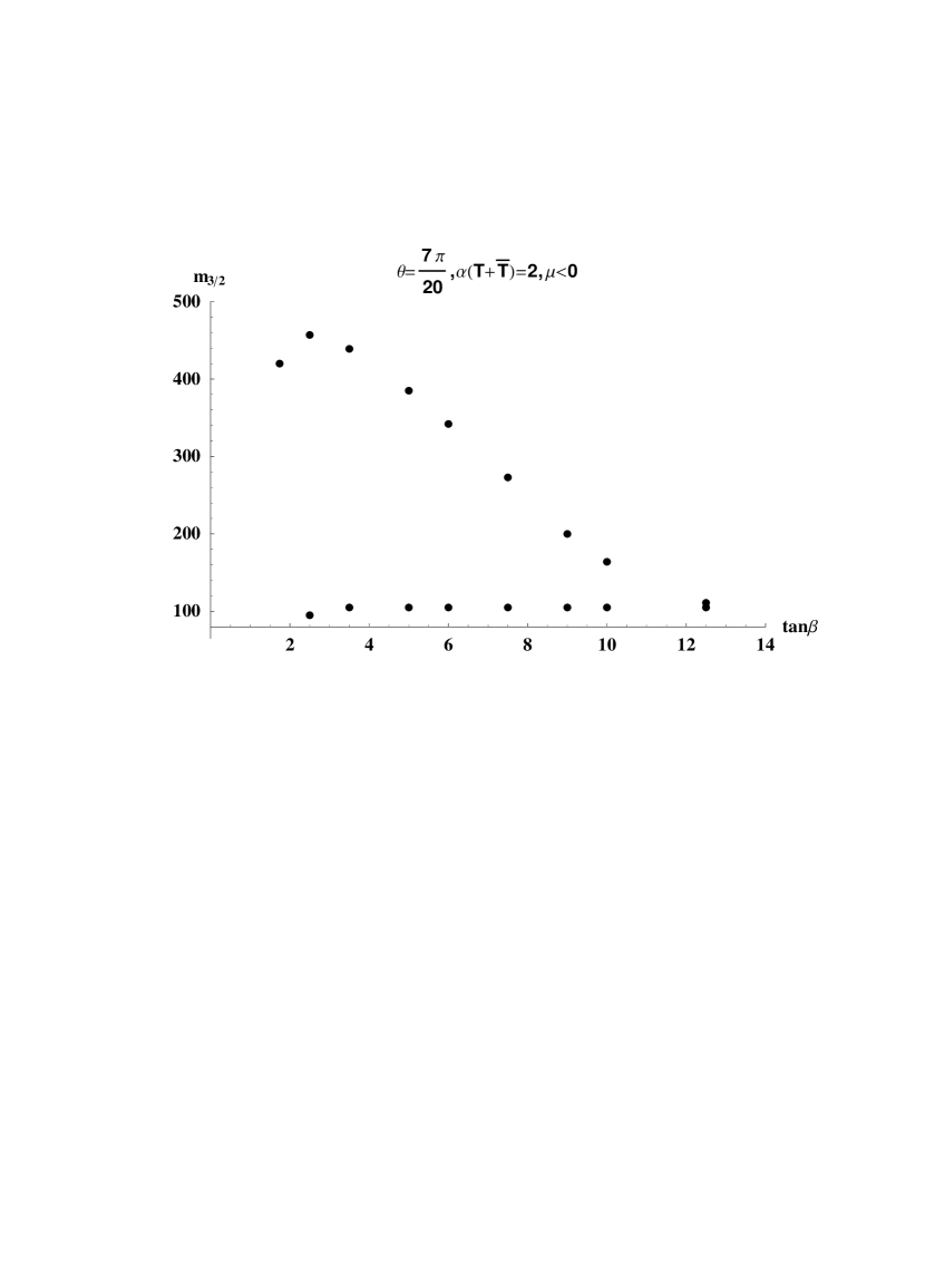
Figure 3: Allowed parameter space in $m_{3/2},\tan\beta$ plane for $\theta=\frac{7\pi}{20},\mu<0$

This of course is phenomenologically unacceptable [4, 20] and results in strong constraints in the sparticle spectrum. In fig.3 we plot the critical value of gravitino mass $m_{3/2}^{c}$ above, (below) which $m_{\tilde{\tau}_{2}}$ or $m_{\tilde{e}_{R}}<m_{\chi_{1}^{0}}$ $(m_{\tilde{\nu}}<43GeV)$ versus $\tan\beta$. The acceptable parameter space lies between the upper and lower bound in fig.3. One can see that because of the above contraint $\tan\beta\leq 13$ in this M-theory limit because the acceptable parameter space vanishes for larger values of $\tan\beta$. We also plot in fig.4 the critical chargino mass $m_{\chi_{1}^{\pm}}$ ,above which the right handed seleptons become the LSP, versus $\tan\beta$. In the same figure we also draw the experimental lower bound for the chargino mass from LEP of about $83$ GeV (horizontal line). The $\tan\beta$ dependence of these constraints may be understood from the $D$-term contribution to the $\tilde{e}_{R}$ and $\tilde{\nu}$ mass formulas

$$\tilde{m}^{2}_{i}=c_{i}m_{3/2}^{2}-d_{i}\frac{\tan^{2}\beta-1}{\tan^{2}\beta+1}M^{2}_{W}$$ (14)

where the $c_{i}$ are some RGE-dependent constants and $d_{\tilde{e}_{R}}=-\tan^{2}\theta_{W}<0$ whereas $d_{\tilde{\nu}}=\frac{1}{2}(1+\tan^{2}\theta_{W})>0$.

In the allowed region of fig.1 the LSP is the lightest neutralino $\chi_{1}^{0}$. Assuming $R$-parity conservation the LSP is stable and consequently can provide a good dark matter candidate. It is a linear combination of the superpartners of the photon, $Z^{0}$ and neutral-Higgs bosons,

$$\chi_{1}^{0}=N_{11}\tilde{B}+N_{12}\tilde{W}^{3}+N_{13}\tilde{H}_{1}^{0}+N_{14}\tilde{H}_{2}^{0}$$ (15)

The neutralino $4\times 4$ mass matrix can be written as

$$\left(\begin{array}[]{cccc}\\ M_{1}&0&-M_{Z}A_{11}&M_{Z}A_{21}\\ 0&M_{2}&M_{Z}A_{12}&-M_{Z}A_{22}\\ -M_{Z}A_{11}&M_{Z}A_{12}&0&\mu\\ M_{Z}A_{21}&-M_{Z}A_{22}&\mu&0\end{array}\right)$$

with

$$\left(\begin{array}[]{cc}\\ A_{11}&A_{12}\\ A_{21}&A_{22}\end{array}\right)=\left(\begin{array}[]{cc}\\ \sin\theta_{W}\cos\beta&\cos\theta_{W}\cos\beta\\ \sin\theta_{W}\sin\beta&\cos\theta_{W}\sin\beta\end{array}\right)$$

In fact the lightest neutralino in this model is almost a pure bino ($\tilde{B}$), which means $f_{g}\equiv|N_{11}|^{2}+|N_{21}|^{2}\gg 0.5$. Most cosmological models predict that the relic abundance of neutralinos [27] satisfies

$$0.1\leq\Omega_{LSP}h^{2}\leq 0.4$$ (16)

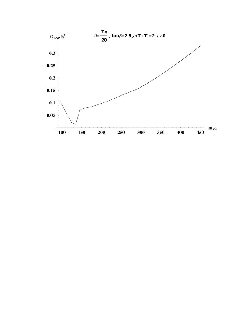
Figure 5: Relic abundance versus $m_{3/2}$ for $\tan\beta=2.5,\mu<0$

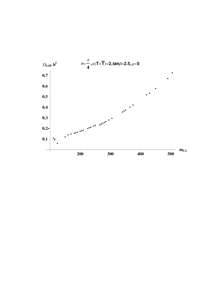
Figure 7: Relic abundance of LSP in case of $\theta=\frac{\pi}{4}$ and $\tan\beta=2.5$

We calculated the relic abundance of the lightest neutralino using standard technology [28] and found strong constraints on the resulting spectrum. In particular for $\mu<0$ the lower limit on the relic abundance results in a lower limit on the gravitino mass of about 200 GeV. In figs(5-7). we plot the relic abundance of the lightest neutralino versus the gravitino mass for various values of $\tan\beta$ for goldstino angle of $\theta=\frac{7\pi}{20}$. We also note that for the allowed parameter space $\Omega_{LSP}h^{2}$ never exceeds the upper limit of 0.4. However, for other values of the goldstino angle the upper limit on $\Omega_{LSP}h^{2}$ can constrain the gravitino mass. The lower limit also constrains the allowed values of the $\tan\beta$ parameter even further. For instance one can see from the plots that $\tan\beta<10$ in order that $\Omega_{LSP}h^{2}\geq 0.1$. In the allowed physical region direct detection rates are of order $10^{-2}-10^{-4}events/Kg/day$. The lightest Higgs mass $m_{h}$ is in the range $87GeV\leq m_{h}\leq 115GeV$, while the neutralino mass is in the range $77GeV\leq m_{\chi_{0}}\leq 195GeV$. At this point is worth mentioning that if one chooses to run the soft masses from the mass $R_{11}^{-1}\sim O(10^{13})GeV$ instead of $7.5\times 10^{15}GeV$ the cosmological constraint ( 16) is very powerful and eliminates all of the parameter space since the relic abundance is always much smaller than 0.1, when $\theta=\frac{7\pi}{20}$. For $\mu>0$ the maximum gravitino mass above which $m_{{\tilde{e}}_{R}}<m_{\chi_{1}^{0}}$ or $m_{{\tilde{\tau}}_{2}}<m_{\chi_{1}^{0}}$ is smaller for fixed $\tan\beta$. Clearly this novel $M$-theory limit provide us with a phenomenology distinct from the weakly coupled case which should be a subject of experimental scrutiny.

For other values of the goldstino angle for which scalar masses are comparable to the gaugino masses (a case which is more similar to the weakly coupled limit [21] in which $m_{0}\sim\frac{1}{\sqrt{3}}M_{1/2}$) we do not obtain constraints from the bounds on the mass of right handed selectrons and staus, but in this case the upper limit on the relic abundance leads to an upper limit on the gravitino mass. For instance, for a goldstino angle of $\theta=\frac{\pi}{4}$ (see fig.7) and $\tan\beta=2.5$, the requirement that $\Omega_{LSP}h^{2}\leq 0.4$ results in $m_{3/2}\leq 365$ GeV. This results in an upper limit for the lightest Higgs mass $m_{h}\leq 100GeV$. The lower limit is now $m_{3/2}\geq 115$ GeV. However, the LEP limit on the chargino mass of 82 GeV requires that $m_{3/2}\geq 150$ GeV. In this case the lightest neutralino is in the range $52GeV\leq m_{\chi_{1}^{0}}\leq 148GeVfor\mu<0$. For $\mu>0$ we have $65GeV\leq m_{\chi_{1}^{0}}\leq 153GeV$. Detection rates of the LSP for ${}^{73}Ge$ detector are in the range $6\times 10^{-2}-10^{-4}events/Kg/day$ for $\mu<0$ and $O(10^{-3})-O(10^{-5}$ events/Kg/day for $\mu>0$. For higher $\tan\beta$ values one can obtain higher detection rates.

For a goldstino angle $\theta=\frac{\pi}{8},\tan\beta=2.5$, the upper limit on the relic abundance leads to an upper limit on the gravitino mass $m_{3/2}\leq 360$ GeV. As a result $m_{\chi_{0}^{1}}\leq 119$GeV and $m_{\chi_{1}^{\pm}}\leq 220$ GeV for $\mu<0$. Similarly, $m_{h}\leq 105$GeV. For higher values of $\tan\beta$, i.e $\tan\beta=15$ the neutralino mass is $60\leq m_{\chi_{1}^{0}}\leq 120$ GeV and $m_{h}\leq 125$ GeV. The detection rates have been calculated in three different nuclei ${}^{73}Ge,^{131}Xe,^{208}Pb$ and are in the range of order $10^{-1}$ to order $10^{-4}events/Kg/day$. The higher the atomic number of the target nuclei the higher the detection rate since the strength of the scalar interaction is sensitive to the atomic number (see Fig.12 and the discussion in section 4). The upper line corresponds to ${}^{208}Pb$ and the lower to ${}^{73}Ge$. Also the higher detection rates occur for low LSP mass ($m_{\chi_{1}^{0}}\sim 60GeV$) since for higher LSP mass the LSP becomes more and more Bino and the interaction is suppressed. The reader should bear in mind the important relationship $m_{\chi_{1}^{0}}\sim\frac{1}{2}m_{\chi_{1}^{\pm}}$ (11). That relationship (11) can provide an important consistency check if a positive signal with $m_{\chi_{1}^{0}}\leq 40$ GeV is found. We also calculated the modulation effect in the total event rate which is small ($\leq 0.05$).

In summary, we have analyzed the supersymmetric spectrum and the properties of the lightest neutralino (LSP) in the 11-dimensional limit of M-theory for the extreme M-theory case in which $\alpha(T+\bar{T})=2$. The most striking result ,in the case of small scalar masses compare with gluino masses, is that one obtains a limit on $\tan\beta\leq 13$, since above that value the right handed selectron or the lightest stau is the LSP, which is phenomenologically unacceptable since the LSP should be electrically neutral [4, 20]. Also the cosmological constraint on the relic abundance of the LSP results in a lower limit on the gravitino mass $m_{3/2}\geq 200$GeV. This further constrains $\tan\beta$; $\tan\beta<10$. In this case the upper limit on the relic abundance is not relevant since $\Omega_{LSP}h^{2}<0.4$ for goldstino angle $\theta=\frac{7\pi}{20}$ and for all the allowed values of $\tan\beta$. Also the lower limit on the relic abundance excludes the case of $R_{11}^{-1}\sim O(10^{13})$ GeV. The scenario with $B_{\mu}$ given by (LABEL:beta), and $\mu$ independent of, $S$ and, $T$ is excluded since one has to go to non-perturbative Yukawa couplings in order to obtain a value of $\tan\beta$ consistent with $B_{\mu}$ as in (LABEL:beta). For a goldstino angle of $\theta=\frac{(7.2)\pi}{20}$ the maximum value of gravitino mass for a fixed $\tan\beta$ is much lower (for $\mu>0$ the parameter space vanishes) from the requirement that the lightest neutralino is the LSP and $\tan\beta(max)\sim 12$. For other values of the goldstino angle (which resemble more the weakly coupled Calabi-Yau compactifications for which $m_{0}=\frac{1}{\sqrt{3}}M_{1/2}$) the upper bound on the relic abundance results in an upper bound on the gravitino mass. For a goldstino angle, $\theta=\frac{\pi}{4}$ and $\tan\beta=2.5$ then we find $m_{3/2}\leq 365$GeV. For $\tan\beta=12.5$ the upper limit on the relic abundance leads to an upper limit on the LSP mass of $\sim 160$ GeV. Direct detection rates of the lightest neutralino are in the range of $10^{-1}-10^{-4}events/Kg/day$.

4 Direct detection

Detection of the LSP is a field in which particle physics, nuclear physics and cosmology play important role in the analysis. Although there are uncertainties which stem from all the above mentioned disciplines the main uncertainty arises from ignorance of the supersymmetric parameters involved. A neutral LSP cannot be detected in collider experiments because of its stability. Experimental detection is therefore focused on underground detectors. There are two main methods, direct detection of the nuclear recoil of order $(10KeV)$ induced by the weak interaction of the LSP with the nucleus [29] and indirect detection which measures the upward muon flux from energetic neutrinos of order 100 GeV resulted from capture of LSP in massive objects like the sun or earth [30].

The typical cross section involved is $\sigma_{0}\sim 10^{-38}cm^{2}$, and for an LSP in the halo with a typical mass of 100GeV interacting with a ${}^{76}Ge$ nucleus of mass 67.9 GeV and moving with a velocity $v$ of 300Km/sec this leads to a detection rate of $\sim 1event/Kg/year$. In what follows we will describe in detail the microscopic interactions of LSP with matter and the process of translating these interactions to the nuclear level[31, 32, 33, 34, 35, 36, 37, 38, 40, 42, 41, 17, 43, 44]. Because the neutralino is a Majorana particle it does not lead to vector interactions with matter because of the identity

$$\bar{\chi_{1}^{0}}\gamma^{\mu}\chi_{1}^{0}=0$$ (17)

This property is important since it makes the observation of LSP a very difficult experimental task. The fundamental interaction of $\chi_{1}^{0}$ with quarks involves three possibilities: exchange of $Z$ boson, s-quark exchange and Higgs exchange. The total interaction is of the form

$${\cal L}_{eff}={\cal L}_{eff}^{(SD)}+{\cal L}_{eff}^{(SI)}$$ (18)

where ${\cal L}_{eff}^{(SD)}$ is a spin dependent interaction and ${\cal L}_{eff}^{(SI)}$ is a spin independent part. In the following we describe in detail the above mentioned three possibilities.

4.1 The $Z$-exchange contribution

This can arise from the interaction of Higgsinos with $Z$. The relevant microscopic Lagrangian reads:

$${\cal L}=\frac{g}{\cos\theta_{W}}\frac{1}{4}(|N_{31}|^{2}-|N_{41}|^{2})\bar{\chi_{1}^{0}}\gamma_{\mu}\gamma_{5}\chi_{1}^{0}Z^{\mu}$$ (19)

Figure 1: Spin dependent scattering of $\chi$ from quarks

which leads to the effective 4-fermion interaction

$${\cal L}_{eff}=\frac{g}{\cos\theta_{W}}\frac{1}{4}2(|N_{31}|^{2}-|N_{41}|^{2})(-\frac{g}{2\cos\theta_{W}}\frac{1}{q^{2}-M_{Z}^{2}}\bar{\chi_{1}^{0}}\gamma^{\mu}\gamma_{5}\chi_{1}^{0})J_{\mu}^{Z}$$ (20)

where $N_{31}$ and $N_{41}$ are defined as in Eq.(15). The neutral hadronic current $J_{\lambda}^{Z}$ is given by

$$J_{\lambda}^{Z}=-\bar{q}\gamma_{\lambda}\Bigl{\{}\frac{1}{3}\sin^{2}\theta_{W}-\Bigl{[}\frac{1}{2}(1-\gamma_{5})-\sin^{2}\theta_{W}\Bigr{]}\tau_{3}\Bigr{\}}q$$ (21)

at the nucleon level it can be written as

$$\tilde{J}_{\lambda}^{Z}=-\bar{N}\gamma_{\lambda}\Bigl{\{}\sin^{2}\theta_{W}-g_{V}(\frac{1}{2}-\sin^{2}\theta_{W})\tau_{3}+\frac{1}{2}g_{A}\gamma_{5}\tau_{3}\Bigr{\}}N$$ (22)

Consequently the effective Lagrangian can be written

$${\cal L}_{eff}=-\frac{G_{F}}{\sqrt{2}}(\bar{\chi_{1}^{0}}\gamma^{\nu}\gamma^{5}\chi_{1}^{0})J_{\nu}(Z)$$ (23)

where

$$J_{\nu}(Z)=\bar{N}\gamma_{\lambda}[f_{V}^{0}(Z)+f_{V}^{1}(Z)\tau_{3}+f_{A}^{0}(Z)\gamma_{5}+f_{A}^{1}(Z)\gamma_{5}\tau_{3}]N$$ (24)

and

$$f_{V}^{0}(Z) = 2(|N_{31}|^{2}-|N_{41}|^{2})\frac{M^{2}_{Z}}{M^{2}_{Z}-q^{2}}\sin^{2}\theta_{W}$$

$$f_{V}^{1}(Z) = -2(|N_{31}|^{2}-|N_{41}|^{2})\frac{M^{2}_{Z}}{M^{2}_{Z}-q^{2}}g_{V}(\frac{1}{2}-\sin^{2}\theta_{W})$$

$$f_{A}^{0}(Z) = 0$$

$$f_{A}^{1}(Z) = 2(|N_{31}|^{2}-|N_{41}|^{2})\frac{M^{2}_{Z}}{M^{2}_{Z}-q^{2}}\frac{1}{2}g_{A}$$ (25)

with $g_{V}=1.0,g_{A}=1.24$. For the Z-exchange (19) we see that this exchange not only depends on the Higgsino component of the neutralino but on their mismatch as well. This interaction is suppressed for an LSP which is almost Bino i.e $\chi_{1}^{0}\sim\tilde{B}$, since the mixing couplings $N_{31},N_{41}$ are small. Nevertheless in some regions of the parameter space $N_{31}\sim 0.2$ and $N_{41}\sim 0.01$ and therefore this interaction is not entirely negligible although much smaller than the scalar interaction.

4.2 The squark mediated interaction

The effective Lagrangian at the nucleon level in this case is given [34] by

$${\cal L}_{eff}=-\frac{G_{F}}{\sqrt{2}}(\bar{\chi}^{0}_{1}\gamma^{\lambda}\gamma^{5}\chi^{0}_{1})J_{\lambda}(\tilde{q})$$ (26)

$$J_{\lambda}(\tilde{q})=\bar{N}\gamma_{\lambda}{f_{V}^{0}(\tilde{q})+f_{V}^{1}(\tilde{q})\tau_{3}+f_{A}^{0}(\tilde{q})\gamma_{5}+f_{A}^{1}(\tilde{q})\gamma_{5}\tau_{3}}N$$ (27)

with

$$f_{V}^{0} = 6(\beta_{0R}-\beta_{0L}),\;\;f_{V}^{1}=2(\beta_{3R}-\beta_{3L})$$

$$f_{A}^{0} = 2g_{V}(\beta_{0R}+\beta_{0L}),\;\;f_{A}^{1}=2g_{A}(\beta_{3R}+\beta_{3L})$$ (28)

with

$$\beta_{0R} = (\frac{4}{9}\chi^{2}_{\tilde{u}_{R}}+\frac{1}{9}\chi^{2}_{\tilde{d}_{R}}|N_{11}\tan\theta_{W}|^{2}$$

$$\beta_{3R} = (\frac{4}{9}\chi^{2}_{\tilde{u}_{R}}-\frac{1}{9}\chi^{2}_{\tilde{d}_{R}}|N_{11}\tan\theta_{W}|^{2}$$

$$\beta_{0L} = |\frac{1}{6}N_{11}\tan\theta_{W}+\frac{1}{2}N_{21}|^{2}\chi^{2}_{\tilde{u}_{L}}+|\frac{1}{6}N_{11}\tan\theta_{W}-\frac{1}{2}N_{21}|^{2}\chi^{2}_{\tilde{d}_{L}}$$

$$\beta_{3L} = |\frac{1}{6}N_{11}\tan\theta_{W}+\frac{1}{2}N_{21}|^{2}\chi^{2}_{\tilde{u}_{L}}-|\frac{1}{6}N_{11}\tan\theta_{W}-\frac{1}{2}N_{21}|^{2}\chi^{2}_{\tilde{d}_{L}}$$ (29)

with

$$\chi^{2}_{qL} = \cos\theta_{\tilde{q}}^{2}\frac{M_{W}^{2}}{m_{\tilde{q_{1}}^{2}}-q^{2}}+\sin\theta^{2}_{\tilde{q}}\frac{M_{W}^{2}}{m_{\tilde{q_{2}}^{2}}-q^{2}}$$

$$\chi^{2}_{qR} = \sin\theta^{2}_{\tilde{q}}\frac{M_{W}^{2}}{m_{\tilde{q_{1}}^{2}}-q^{2}}+\cos\theta_{\tilde{q}}^{2}\frac{M_{W}^{2}}{m_{\tilde{q_{2}}^{2}}-q^{2}}$$ (30)

where $\tilde{q}_{1,2}$ are the squark mass eigenstates and $\theta_{\tilde{q}}$ the squark mass matrices mixing angles.

4.3 The intermediate Higgs contribution

The scalar interaction receives contributions from Higgs exchange and from the squark exchange. We first describe the Higgs exchange.

$${\cal L}_{H\chi_{1}^{0}\chi_{1}^{0}} = \frac{g}{\sqrt{2}}((N_{21}-\tan\theta_{W}N_{11})N_{41}\bar{\chi}^{0}_{1R}\chi_{1L}^{0}H_{2}^{0*}$$ (31)

$$- (N_{21}-\tan\theta_{W}N_{11})N_{31}\bar{\chi}^{0}_{1R}\chi_{1L}^{0}H_{1}^{0*})+{\rm h.c}$$

Figure 2: Diagrams contributing to the scalar scattering of $\chi$ with quarks

If we express the fields $H_{1}^{0*},H_{2}^{0*}$ in terms of the mass eigenstates $h,H,A$ we get

$${\cal L}_{eff}=-\frac{G_{F}}{\sqrt{2}}\bar{\chi}_{1}^{0}\chi_{1}^{0}\bar{N}[f_{s}^{0}(H)+f_{s}^{1}(H)\tau_{3}]N$$ (32)

where

$$f_{s}^{0}(H)=\frac{1}{2}(g_{u}+g_{d})+g_{s}+g_{c}+g_{b}+g_{t}$$ (33)

$$f_{s}^{1}(H)=\frac{1}{2}(g_{u}-g_{d})$$ (34)

with

$$g_{a_{i}}=\Bigl{[}g_{1}(h)\frac{\cos\alpha}{\sin\beta}+g_{2}(H)\frac{\sin\alpha}{\sin\beta}\Bigr{]}\frac{m_{a_{i}}}{m_{N}},a_{i}=u,c,t$$ (35)

$$g_{f_{i}}=\Bigl{[}-g_{1}(h)\frac{\sin\alpha}{\cos\beta}+g_{2}(H)\frac{\cos\alpha}{\cos\beta}\Bigr{]}\frac{m_{f_{i}}}{m_{N}},\;f_{i}=d,s,b$$ (36)

$$g_{1}(h)=4(N_{11}\tan\theta_{W}-N_{21})(N_{41}\cos\alpha+N_{31}\sin\alpha)\frac{m_{N}M_{W}}{m^{2}_{h}-q^{2}}$$ (37)

$$g_{2}(H)=4(N_{11}\tan\theta_{W}-N_{21})(N_{41}\sin\alpha-N_{31}\cos\alpha)\frac{m_{N}M_{W}}{m_{H}^{2}-q^{2}}$$ (38)

where $m_{N}$ is the nucleon mass, $m_{h},m_{H}$ are the one-loop corrected lightest and heavier Higgs CP-even mass eigenstates and $\alpha$ is the Higgs mixing angle which at tree level is given by

$$\cos{2\alpha}=-\cos 2\beta\Biggl{(}\frac{m^{2}_{A}-M^{2}_{Z}}{m^{2}_{H}-m^{2}_{h}}\Biggr{)}$$ (39)

However, we determine the Higgs mixing angle numerically by diagonalizing the one-loop $CP$-even Higgs mass matrix since as has been emphasized in [36] the determination of the Higgs mixing angle by inserting the one-loop values in the tree-level expression (39) leads to erroneous results.

We note that the scalar interaction involves an interference of the gaugino and the Higgsino components. Thus if the LSP were to be strictly a Bino or a Higgsino , the scalar interaction would vanish and the neutralino-nucleus scattering would be strictly governed by the spin dependent interaction. However, such a situation is never realized and the scalar interaction plays the dominant role in the event rate analysis of the effective supergravity from $M$-theory. At this point we must emphasize that the coherent interaction depends very much on the nuclear model. If only the up and down quarks contribute to the nucleon mass and $m_{u}=5MeV,m_{d}=10MeV$ one finds [45]

$$f_{s}^{0}=1.86(g_{u}+g_{d})/2,f_{s}^{1}=0.49(g_{u}-g_{d})/2$$ (40)

In this case the interaction is small. However, if heavier quarks are also involved due to QCD effects, one obtains the pseudoscalar Higgs-nucleon interaction $f_{s}^{0}(H)$ by using effective quark masses as follows

$$m_{u}\rightarrow f_{u}m_{N},\;\;m_{d}\rightarrow f_{d}m_{N},m_{s}\rightarrow f_{s}m_{N},m_{Q}\rightarrow f_{Q}m_{N}\;\;{\rm for}\;{\rm heavy}\;{\rm quarks}\;\;(c,b,t)$$ (41)

where $m_{N}$ is the nucleon mass. The isovector contribution is now negligible. The parameters $f$ can be obtained by chiral symmetry breaking terms in relation to phase shift and dispersion analysis. Following Cheng we obtain

$$f_{u}=0.021,\;f_{d}=0.037,\;f_{s}=0.140$$ (42)

As pointed by Shifman, Vainstein, and Zakharov, heavy quarks contribute to the mass of the nucleon through the anomaly [46]. Under the heavy quark expansion, the following substitution can be made for the heavy quarks $Q=c,b,t$, in a nucleon matrix element [46]

$$m_{Q}\bar{Q}Q\rightarrow\frac{-2\alpha_{S}}{24\pi}GG$$ (43)

so we find that for each of the heavy quarks, $Q=c,b,t$ [28],

$$<N|m_{Q}\bar{Q}Q|N>=\frac{2}{27}m_{N}\Bigl{[}1-\sum_{q=u,d,s}f^{N}_{q}\Bigr{]}$$ (44)

with $G$ the QCD field strength.

In the case of the scalar interaction, the sum over all quarks in the nucleus produces a mass factor $A$, which enhances the contribution of the scalar term. Thus the heavier the nucleus the more sensitive it is to the spin-independent scattering.

We can also a have a small scalar contribution from the squark exchange, as was first observed by Griest [31], in which the effective Lagrangian at the nucleon level is

$${\cal L}=\frac{G_{F}}{\sqrt{2}}[f_{S}^{0}(\tilde{q})\bar{N}N+f_{s}^{1}(\tilde{q})\bar{N}\tau_{3}N]\bar{\chi}_{1}^{0}\chi_{1}^{0}$$ (45)

with $f_{s}^{0}(\tilde{q})=1.86\beta_{+}$ and $f_{s}^{1}(\tilde{q})=0.48\beta_{-}$ [45] with

$$\beta_{\pm} = \frac{1}{3}\tan\theta_{W}N_{11}\{2\sin 2\theta_{\tilde{u}}[\frac{1}{6}N_{11}\tan\theta_{W}+\frac{1}{2}N_{21}]\Delta_{\tilde{u}}$$ (46)

$$\mp \sin 2\theta_{\tilde{d}}[\frac{1}{6}N_{11}\tan\theta_{W}-\frac{1}{2}N_{21}]\Delta_{\tilde{d}}\}$$

4.4 The nuclear matrix elements

Combining the results of the previous subsections we can write

$${\cal L}_{eff}=-\frac{G_{F}}{\sqrt{2}}\Bigl{\{}(\bar{\chi}_{1}^{0}\gamma^{\lambda}\gamma_{5}\chi_{1}^{0})J_{\lambda}+(\bar{\chi}_{1}^{0}\chi_{1}^{0})J\Bigr{\}}$$ (47)

where

$$J_{\lambda}=\bar{N}\gamma_{\lambda}(f_{V}^{0}+f_{V}^{1}\tau_{3}+f_{A}^{0}\gamma_{5}+f_{A}^{1}\gamma_{5}\tau_{3})N$$ (48)

with

$$f_{V}^{0} = f_{V}^{0}(Z)+f_{V}^{0}(\tilde{q}),\;\;f_{V}^{1}=f_{V}^{1}(Z)+f_{V}^{1}(\tilde{q})$$

$$f_{A}^{0} = f_{A}^{0}(Z)+f_{A}^{0}(\tilde{q}),\;\;f_{A}^{1}=f_{A}^{1}(Z)+f_{A}^{1}(\tilde{q})$$ (49)

and the scalar interaction is given by

$$J=\bar{N}(f_{s}^{0}+f_{s}^{1}\tau_{3})N$$ (50)

The total cross section can be cast in the form [28, 43]

$$\sigma = \sigma_{0}(\frac{m_{\chi_{1}^{0}}}{m_{N}})^{2}(\frac{1}{(1+\eta)^{2}}\Bigl{\{}A^{2}[[\beta^{2}(f_{V}^{0}-f_{V}^{1}\frac{A-2Z}{A})^{2}$$ (51)

$$+ (f_{s}^{0}-f_{s}^{1}\frac{A-2Z}{A})^{2}]I_{0}(u_{0})-\frac{\beta^{2}}{2}\frac{2\eta+1}{(1+\eta)^{2}}(f_{V}^{0}-f_{V}^{1}\frac{A-2Z}{A})^{2}I_{1}(u_{0})]$$

$$+ (f_{A}^{0}\Omega_{0}(0))^{2}S_{00}(u_{0})+2f_{A}^{0}f_{A}^{1}\Omega_{0}(0)\Omega_{1}(0)S_{01}(u_{0})$$

$$+ (f_{A}^{1}\Omega_{1}(0))^{2}S_{11}(u_{0})\Bigr{\}}$$

where

$$\sigma_{0}=\frac{1}{2\pi}(G_{F}m_{N})^{2}\sim 0.77\times 10^{-38}cm^{2}$$ (52)

and

$$\eta=\frac{m_{\chi^{0}_{1}}}{m_{N}A};q_{0}=\beta\frac{2m_{\chi^{0}_{1}}c}{1+\eta}$$ (53)

and the dimensionless quantity $u_{0}$ is defined as [43]

$$u_{0}=q_{0}^{2}b^{2}/2$$ (54)

with $b\sim 1.0A^{1/6}\rm{fm}$ and $A=Z+N$ is the atomic number of the nuclei. The form factors entering (51) are defined as

$$I_{\rho}=(1+\rho)u_{0}^{-(1+\rho)}\int_{0}^{\infty}x^{1+\rho}|F(x)|^{2}dx,\;\;\rho=0,1$$ (55)

where $F(q)$ is the nuclear form factor. Another appropriate form factor is the Woods-Saxon form factor [47]

$$I_{WS}=\frac{3j_{1}(qR_{0})}{qR_{0}}exp[-\frac{1}{2}(qs)^{2}]$$ (56)

or using appropriate expressions for the form factors [39](in a harmonic oscillator basis with size parameter $b$)

$$I_{\rho}=\frac{1}{A^{2}}\Bigl{\{}Z^{2}I_{ZZ}^{(\rho)}(u_{0})+2NZI_{NZ}^{(\rho)}(u_{0})+N^{2}I_{NN}^{(\rho)}(u_{0})\Bigr{\}}$$ (57)

where

$$I_{\alpha\beta}^{(\rho)}(u_{0}) = (1+\rho)\;\sum_{\lambda=0}^{N_{max(\alpha)}}\sum_{\nu=0}^{N_{max(\beta)}}\frac{\theta_{\lambda}^{(\alpha)}}{\alpha}\frac{\theta_{\nu}^{(\beta)}}{\beta}\frac{2^{\lambda+\nu+\rho}(\lambda+\nu+\rho)!}{u_{0}^{1+\rho}}$$ (58)

$$\times [1-e^{-u_{0}}\sum_{k=0}^{\lambda+\nu+\rho}\frac{u_{0}^{\kappa}}{\kappa!}]$$

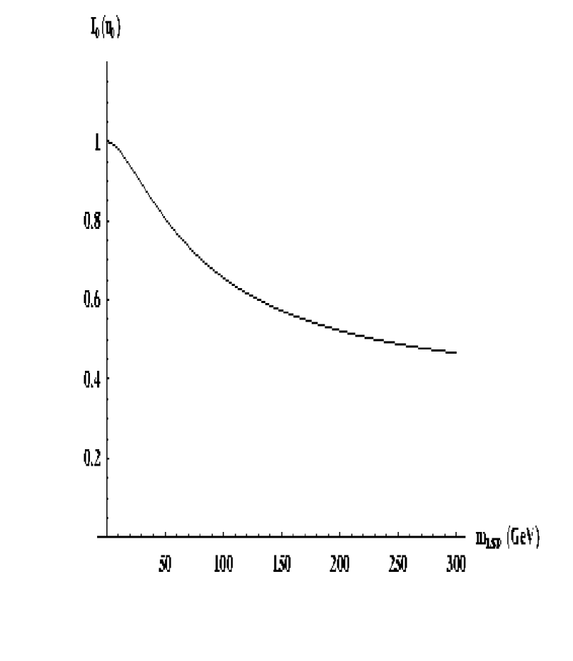
Figure 8: Form factor $I_{0}(u_{0})$ versus LSP mass for ${}^{72}_{32}Ge$ nuclei see Eq.(57)

We exhibit the dependence of the scalar form factors $I_{0}$ on the LSP mass in fig. (8)-(10) for three different nuclei.

Since the LSP is moving with velocity $v_{Z}$ with respect to the detector nuclei the detection rate for a target with mass $m$ is given by

$$R=\frac{dN}{dt}=\frac{\rho_{0}}{m_{\chi_{1}^{0}}}\frac{m}{Am_{p}}\int f(\bf{v})|v_{z}|\sigma(|\bf{v}|)d^{3}\bf v$$ (59)

where $\rho_{0}=0.3GeV/cm^{3}$ is the local LSP density in our vicinity which has to be consistent with a Maxwell distribution

$$f(v^{\prime})d^{3}v^{\prime}=(\sqrt{\pi}v_{0})^{(-3)}e^{(-v^{\prime}/v_{0})^{2}}d^{3}v^{\prime}$$ (60)

and

$$v_{0}=\sqrt{(2/3)<v^{2}>}=220Km/s$$ (61)

More realistically, one should take into account the motion of the Sun and Earth. This increases the total event rate and gives rise to a yearly modulation in the event rate which might serve as a method of distinguishing signal from noise if many events are found [48]. Following Freese, Frieman and Gould and Sadoulet [48], one subtracts the Earth velocity $\bf{v_{E}}$ from $v^{\prime}$ in (60) to get the velocity $v$ of the LSP in the Earth frame.

$${{\bf v^{\prime}}=\bf{v}+\bf{v_{E}}},\;\;{v^{\prime}}^{2}=v^{2}+v^{2}_{E}+2vv_{E}\cos\chi$$ (62)

where $\chi$ is the angle between the LSP velocity in the Earth frame and the direction of the Earth’s motion. As a function of time, $v_{E}$ changes as the Earth’s motion comes into and out of alignment and the event rate peaks around second of June. This is taken into account using

$$v_{E}=v_{0}\Bigl{[}1.05+0.07\cos\Bigl{(}\frac{2\pi(t-t_{p})}{\rm{1yr}}\Bigr{)}\Bigr{]}$$ (63)

where $t_{p}=\rm{June}2^{nd}\pm 1.3days$. Changing variables, and integrating over angles one obtains

$$f_{1}(v)dv=\frac{vdv}{v_{E}v_{0}\sqrt{\pi}}\Bigl{\{}e^{-\frac{(v-v_{e})^{2}}{v_{0}^{2}}}-e^{-\frac{(v+v_{E})^{2}}{v_{0}^{2}}}\Bigr{\}}$$ (64)

Assuming a Gaussian parametrization for the form factors [32] and averaging over the Maxwellian distribution of dark matter velocities the total scattering rate is given by

$$R = (R_{S.I}+R_{S.D})\frac{4m_{\chi_{1}^{0}}m_{A}}{(m_{\chi_{1}^{0}}+m_{A})^{2}}$$ (65)

$$\times \frac{\rho_{0}}{0.3GeVcm^{-3}}\frac{|V_{E}|}{320kms^{-1}}\frac{events}{Kgd}$$

where the

$$R_{S.I} = 840m_{A}^{2}M_{Z}^{4}\zeta|A_{S.I}|^{2}$$ (66)

and

$$\zeta = \frac{0.573}{b}\Bigl{(}1-\frac{exp[-b/(1+b)]}{\sqrt{1+b}}\frac{\rm{erf}(1/\sqrt{1+b})}{\rm{erf}(1)}\Bigr{)}$$ (67)

is a form factor with

$$b=\frac{m_{\chi_{1}^{0}}^{2}m_{A}^{2}}{((m_{\chi_{1}^{0}}+m_{A})^{2}}\frac{8}{9}\sigma^{2}r^{2}_{charge}$$ (68)

where $\sigma=0.9\;10^{-3}$ is the velocity dispersion and $r_{charge}=(0.3+0.89A^{1/3})\rm{fm}$.

5 Conclusions

In this work we have analysed the supersymmetric particle spectrum of the extreme M-theory case $(\alpha(T+\bar{T})=2)$ with the requirement that the lightest supersymmetric particle is the dominant component of the dark matter in the universe. We also calculated in detail the detection rates of direct interaction of neutralinos with various nuclei ${}^{131}Xe,^{73}Ge,^{208}Pb$. The LSP in the effective supergravity from M-theory is almost a Bino. This has the important effect that the scalar component (through Higgs exchange) is the dominant interaction of the LSPs with terrestrial nuclei. The strength of this interaction is such that this should be detectable in the near future by nuclei with large atomic number $A$, since these nuclei are more sensitive to the scalar interaction as illustrated in Fig.12. We obtain maximum event rates of order $50events/Kg/year$ for large values of $\tan\beta$ and lightest chargino mass of order $100$ GeV. The detection rates depend also on the sign of the $\mu$ parameter as well the nucleon model . Therefore the allowed parameter space can be limited by experimental investigation. We also calculated the magnitude of the modulation effect due to the annual revolution of Earth which is small ($\leq 0.05$).

In the scenario with small scalar masses compare to gaugino masses, i.e $m_{0}\ll M_{1/2}$ the parameter $\tan\beta$ is constrained to be small, i.e $\tan\beta\leq 12$ from the requirement that the LSP should be the lightest neutralino. After imposing the limits on the relic abundance of the lightest neutralino the upper limit on $\tan\beta$ becomes smaller ($\tan\beta\leq 10$).

For scenarios with scalar masses comparable to the gaugino masses at the unification scale the upper limit from cosmology on the relic abundance of the LSP imposes an upper bound on the gravitino mass and gluino masses.

The above results motivate the investigation of the effect of CP violating phases in the soft supersymmetry-breaking terms on the detection rates as well as the investigation of the size of the modulation effect on the differential event rate. The above will be the subject of a future publication [49].

Figure 4: Maximum lightest chargino mass vs $\tan\beta$

Figure 6: Relic abundance of LSP vs $m_{3/2}$ for $\tan\beta=5,\mu<0$

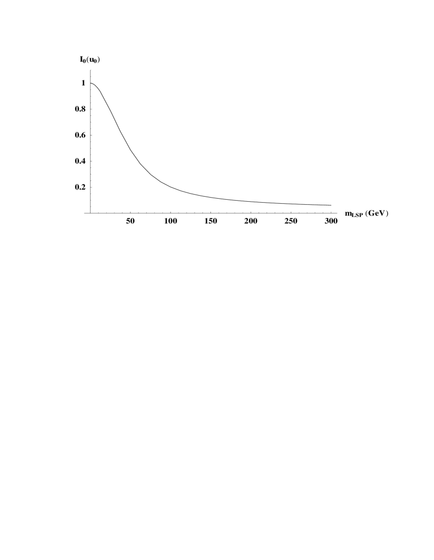
Figure 9: Form factor $I_{0}(u_{0})$ versus LSP mass for ${}^{208}_{82}Pb$ nuclei see Eq.(57)

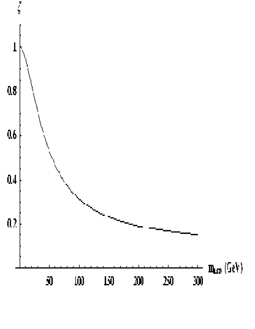
Figure 10: Form factor $\zeta$ for ${}^{131}Xe$ nuclei

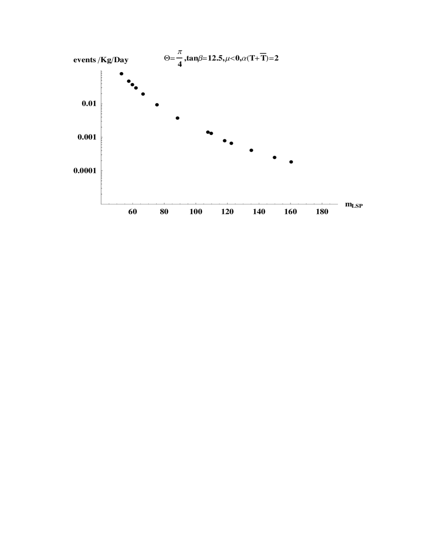
Figure 11: Detection rates in the case $\theta=\frac{\pi}{4},\tan\beta=2.5$

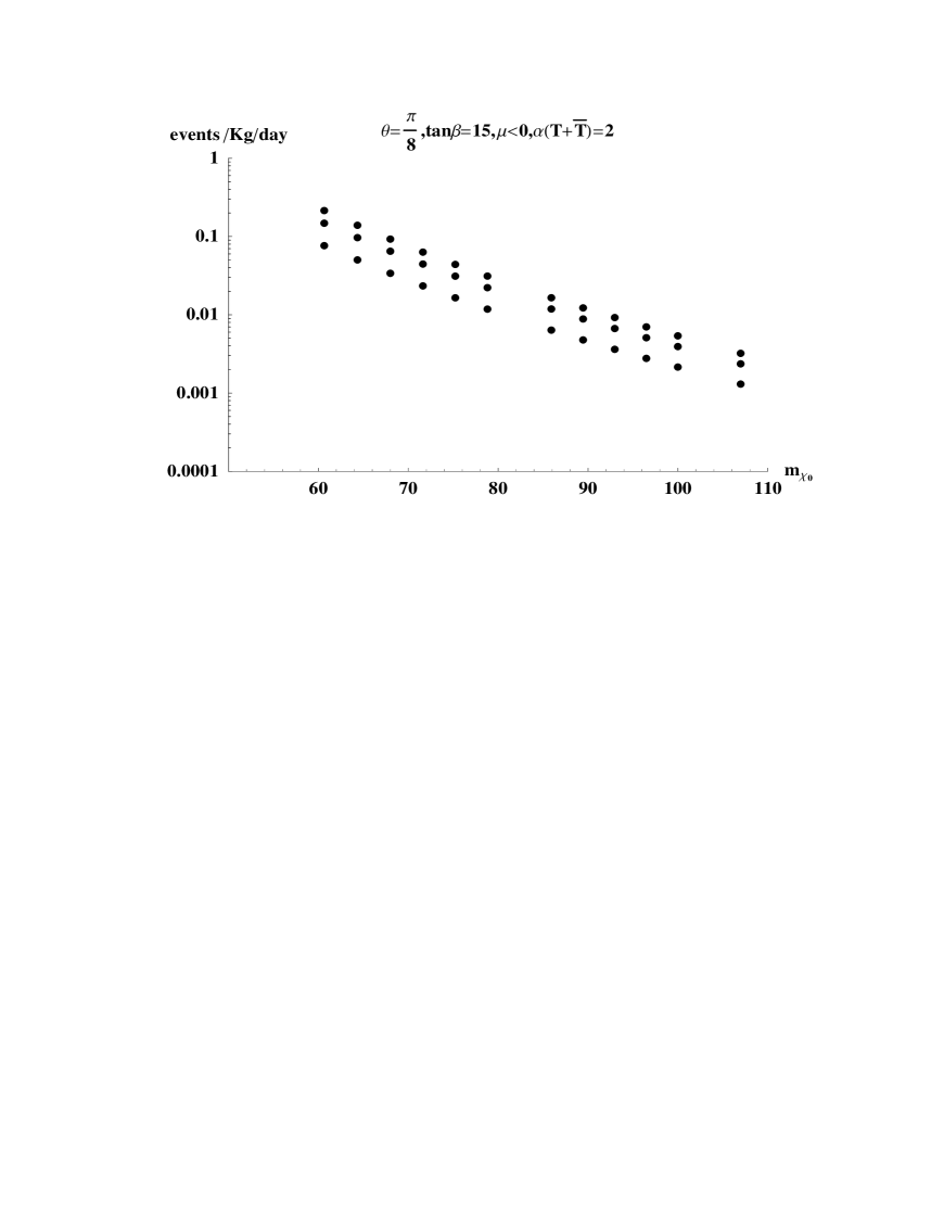
Figure 12: Event rates for 3 different nuclei,${}^{208}Pb,^{131}Xe,^{73}Ge$

References

• [1] P. Ho${\rm{\breve{r}}}$ava and E. Witten, Nucl. Phys. B460(1996)506; Nucl. Phys. B475(1996)94
• [2] M. Faux, hep-th/9801204
• [3] E. Witten, Nucl. Phys. B471(1996)135
• [4] J. Ellis, J.S. Hagelin, D.V. Nanopoulos, K.A. Olive and M. Srednicki, Nucl.Phys.B238(1984)453
• [5] E. Daw, “Results for the large scale US axion search”, To be published in the Proc.of IDM98, Buxton,UK
• [6] R. Bernabei et al, Phys. Lett.B424(1998)195; R. Bernabei et al.,preprint ROM2F/98/27, August 1998
• [7] K. Benakli, J. Ellis and D. V. Nanopoulos, hep-ph/9803333
• [8] I. Antoniadis and M. Quir${\rm{\acute{o}}}$s, Phys.Lett.B392(1997)61;hep-th/9705037
• [9] T. Li, J.L. Lopez and D.V. Nanopoulos,hep-ph/9702237; hep-ph/9704247; D.V. Nanopoulos, hep-th/9711080
• [10] T. Li,hep-th/9801123
• [11] H.P. Nilles, M. Olechowski and M. Yamaguchi,hep-ph/9707143, Phys. Lett.B415(1997)24; H.P. Nilles, M. Olechowski and M. Yamaguchi,hep-th/9801030;Y. Kawamura, H.P. Nilles, M. Olechowski and M. Yamaguchi,hep-ph/9805397
• [12] E. Dudas and C. Grojean,hep-th/9704177; E. Dudas,hep-th/9709043
• [13] Z. Lalak and S. Thomas, hep-th/9707223
• [14] K. Choi, H.B. Kim and C. Mu${\rm\tilde{n}}$oz, hep-th/9711158
• [15] A. Lukas, B.A. Ovrut and D. Waldram, hep-th/9711197; A. Lukas, B.A. Ovrut and D. Waldram, hep-th/9710208; A. Lukas, B.A. Ovrut, K.S. Stelle and D. Waldram, hep-th/9806051; A. Lukas, B.A. Ovrut and D. Waldram, hep-th/9812052
• [16] L. Ibanez, G.G. Ross: Phys. Lett. B110 (1982) 215; L. Alvarez-Gaume, J. Polchinsky and M. Wise: Nucl. Phys. B221 (1983) 495; J. Ellis, J.S. Hagelin, D.V. Nanopoulos and K. Tamvakis: Phys. Lett. B125 (1983) 275; M. Claudson, L. Hall and I. Hinchliffe: Nucl. Phys. B228 (1983) 501; C. Kounnas, A.B. Lahanas, D.V. Nanopoulos and M. Quiros: Nucl. Phys. B236 (1984) 438; L.E. Ib$\acute{a}$ $\tilde{n}$ez and C. Lopez: Nucl. Phys. B233 (1984) 511; A. Bouquet, J. Kaplan, C.A. Savoy: Nucl. Phys. B262 (1985) 299
• [17] D. Bailin, G.V. Kraniotis and A. Love, Phys.Lett.B432(1998)90
• [18] C.E. Huang, T. Liao, Q. Yan and T. Li, hep-ph/9810412
• [19] J.A. Casas, A. Ibarra and C. Munoz,hep-ph/9810266
• [20] S. Wolfram, Phys.Lett.B82(1979)65; P.F. Smith and J. R. J. Bennett, Nucl.Phys.B149(1979)525
• [21] A. Brignole, L.E. Ib$\rm{\acute{a}}\rm{\tilde{n}}$ez and C. Munoz, Nucl. Phys.B422(1994)125
• [22] S. Kachru, Phys.Lett.B349(1995)76
• [23] K. Benakli, hep-th/9805181
• [24] S. Stieberger, hep-th/9807124, To appear in Nucl.Phys.B
• [25] D. Bailin, G.V. Kraniotis and A. Love, Phys. Lett.B414(1997)269; D. Bailin, G.V. Kraniotis and A. Love, Nucl.Phys.B518(1998)92
• [26] P. Nath and R. Arnowitt, Phys. LettB289(1992)368
• [27] R. Arnowitt and P. Nath, Phys. Rev. D56 (1997)2820; hep-ph/9701301
• [28] G. Jungman, M. Kamionkowski and K. Griest, Phys. Rep. 267(1996) 195
• [29] M.W. Goodman and E. Witten, Phys.Rev.D31 (1986)3059
• [30] J. Silk, K. Olive and M. Srednicki, Phys.Rev.Lett.55(1985)257; L. M. Krauss, K. Freese, D. N. Spergel and W. H. Press, Astrophys.J.299(1985)1001;L. M. Krauss, M. Srednicki and F. Wilczek, Phys.Rev.D33(1986)2079
• [31] K. Griest, Phys.Rev.Lett.62(1988)666;Phys.Rev.D38(1988)2357; D39(1989)3802
• [32] J. Ellis and R. Flores,Phys.Lett.B300(1993)175
• [33] A. Bottino et al,Astro.Part.Phys.1(1992)61;2(1994)77
• [34] M. Drees and M. Nojiri, Phys.Rev.D48(1993)3483
• [35] V.A. Bednyakov, H. V. Klapdor-Kleingrothaus and S.G. Kovalenko, Phys.Rev.D50(1994)7128
• [36] P. Nath and R. Arnowitt, Phys.Rev.Lett.74(1995)4592; R. Arnowitt and P. Nath, Mod. Phys. Lett. A10 (1995) 1257
• [37] E. Diehl, G. Kane, C. Kolda and J. Wells,Phys.Rev.D52(1995)4223
• [38] L. Bergstrom and P. Gondolo,hep-ph/9510252
• [39] T. S. Kosmas and J. D. Vergados,nucl-th/9509026
• [40] J.D. Vergados, J. Phys. G22(1996)253
• [41] G.L. Kane and J.D. Wells, Phys.Rev.Lett.76(1996)4458
• [42] B. de Carlos and G.V. Kraniotis, Proc. of IDM 96; Sheffield(1996) 581-586;hep-ph/9610355
• [43] J.D. Vergados and T.S. Kosmas,hep-ph/9802270
• [44] S. Khalil, A. Masiero and Q. Shafi, Phys.Rev.D56(1997)5754; Phys.Lett.B397(1997)197
• [45] S.L. Addler, Phys.Rev.D 11 (1975)3309
• [46] M.A. Shifman, A.I. Vainshtein and V.I. Zakharov, Phys.Lett.B78 (1978)443
• [47] J. Engel,Phys.Lett.B264(1991)114
• [48] K. Freese, J. Frieman and A. Gould, Phys.Rev.D37(1988)3388
• [49] G. V. Kraniotis, in preparation
Refer to caption