Abstract

We determine the three-neutrino mixing and mass parameters that are allowed by the solar and atmospheric neutrino data when vacuum oscillations are responsible for both phenomena. The global fit does not appreciably change the allowed regions for the parameters obtained from effective two-neutrino fits. We discuss how measurements of the solar electron energy spectrum below 6.5 GeV in Super-Kamiokande and seasonal variations in the Super-Kamiokande, ⁷¹Ga, and BOREXINO experiments can distinguish the different solar vacuum solutions.

I Introduction

Recent data from the Super-Kamiokande experiment [1, 2] have strengthened the interpretation of the solar [3, 4, 5, 6] and atmospheric [8, 9] neutrino anomalies in terms of neutrino oscillations. Oscillations have also been invoked to describe the appearance of electron neutrinos and antineutrinos in the LSND experiment [10]. Because confirmation of the LSND results awaits future experiments and recent measurements in the KARMEN detector exclude part of the LSND allowed region [11], a conservative approach is to assume that oscillations need only account for the solar and atmospheric data. Then the two mass-squared difference scales in a three-neutrino model are sufficient to describe the data. A number of three-neutrino models have been investigated [12, 13, 14, 15, 16, 17]. One attractive possibility is that both the atmospheric $\nu_{\mu}$ and solar $\nu_{e}$ oscillate maximally [14] or near-maximally [15] at the $\delta m^{2}_{atm}$ and $\delta m^{2}_{sun}$ scales, respectively.

Most detailed oscillation fits have been done separately for the solar and atmospheric data in effective two-neutrino approximations [18]. In this paper we make full three-neutrino fits to the solar and atmospheric oscillation data to determine the allowed values for the general three-neutrino mixing matrix under the assumption that one mass-squared difference, $\delta m^{2}_{atm}$, explains the atmospheric neutrino oscillations and that the other independent mass-squared difference, $\delta m^{2}_{sun}\ll\delta m^{2}_{atm}$, explains the solar neutrino oscillations via the vacuum long-wavelength scenario [19, 20]. We choose a particular parametrization for the three-neutrino mixing in which the expressions for the atmospheric and solar neutrino oscillations share only a single parameter, and discuss the degree to which the two phenomena decouple. We find that the extension from two to three neutrino species does not improve the separate fits to either the atmospheric or solar data. Although pure $\nu_{\mu}\rightarrow\nu_{\tau}$ oscillations of atmospheric neutrinos are favored, there exist three-neutrino solutions with non-negligible $\nu_{\mu}\leftrightarrow\nu_{e}$ oscillations, even with the constraints from the CHOOZ reactor experiment [21]. Hence both $\nu_{\mu}\leftrightarrow\nu_{e}$ and $\nu_{e}\rightarrow\nu_{\tau}$ oscillations may be observable in future long-baseline experiments. We also find that future measurements of seasonal variations in the solar neutrino signal can provide an unmistakable sign of vacuum oscillations, and can further constrain the allowed parameter regions.

In Sec. II we review the formalism for oscillations of three neutrinos relevant to the atmospheric and solar phenomena. In Sec. III we evaluate the current allowed two-neutrino parameter regions, and briefly review the evidence indicating that two distinct $\delta m^{2}$ are needed to describe the solar and atmospheric data. In Sec. IV we obtain three-neutrino solutions from a combined fit to the atmospheric and solar data. We conclude with a discussion of future tests of vacuum oscillations in Sec. V.

II Oscillation analysis

A General probability expressions

The survival probability for a given neutrino flavor $\nu_{\alpha}$ in a vacuum is [22]

$$P(\nu_{\alpha}\to\nu_{\alpha})=1-4\sum_{k<j}|U_{\alpha j}|^{2}|U_{\alpha k}|^{2}\sin^{2}\Delta_{jk}\,,$$ (1)

where $U$ is the neutrino mixing matrix (in the basis where the charged-lepton mass matrix is diagonal), $\Delta_{jk}\equiv\delta m_{jk}^{2}\,L/4E=1.27(\delta m^{2}_{jk}/{\rm eV}^{2})(L/{\rm km})/(E/{\rm GeV})$, $\delta m^{2}_{jk}\equiv m^{2}_{j}-m^{2}_{k}$, and the sum is over all $j$ and $k$, subject to $k<j$. The matrix elements $U_{\alpha j}$ are the mixings between the flavor ($\alpha=e,\mu,\tau$) and the mass ($j=1,2,3$) eigenstates, and we assume without loss of generality that $m_{1}<m_{2}<m_{3}$. The solar oscillations are driven by $|\Delta_{21}|\equiv\Delta_{sun}$ and the atmospheric oscillations are driven by $|\Delta_{31}|\simeq|\Delta_{32}|\equiv\Delta_{atm}\gg\Delta_{sun}$.

The off-diagonal vacuum oscillation probabilities in a three-neutrino model are [23]

$$P(\nu_{e}\rightarrow\nu_{\mu}) = 4\,|U_{e3}U_{\mu 3}^{*}|^{2}\sin^{2}\Delta_{atm}-4Re\{U_{e1}U_{e2}^{*}U_{\mu 1}^{*}U_{\mu 2}\}\sin^{2}\Delta_{sun}-2\,J\sin 2\Delta_{sun}\,,$$ (2)

$$P(\nu_{e}\rightarrow\nu_{\tau}) = 4\,|U_{e3}U_{\tau 3}^{*}|^{2}\sin^{2}\Delta_{atm}-4Re\{U_{e1}U_{e2}^{*}U_{\tau 1}^{*}U_{\tau 2}\}\sin^{2}\Delta_{sun}+2\,J\sin 2\Delta_{sun}\,,$$ (3)

$$P(\nu_{\mu}\rightarrow\nu_{\tau}) = 4\,|U_{\mu 3}U_{\tau 3}^{*}|^{2}\sin^{2}\Delta_{atm}-4Re\{U_{\mu 1}U_{\mu 2}^{*}U_{\tau 1}^{*}U_{\tau 2}\}\sin^{2}\Delta_{sun}-2\,J\sin 2\Delta_{sun}\,,$$ (4)

where the $CP$-violating “Jarlskog invariant” [24] is $J=\sum_{k,\gamma}\epsilon_{ijk}\epsilon_{\alpha\beta\gamma}Im\{U_{\alpha i}U_{\alpha j}^{*}U_{\beta i}^{*}U_{\beta j}\}$ for any $\alpha$, $\beta$, $i$, and $j$ (e.g., $J=Im\{U_{e2}U_{e3}^{*}U_{\mu 2}^{*}U_{\mu 3}\}$ for $\alpha=e$, $\beta=\mu$, $i=2$, and $j=3$). The $CP$-odd term changes sign under reversal of the oscillating flavors, or if neutrinos are replaced by anti-neutrinos. We note that the $CP$-violating probability at the atmospheric scale is suppressed to order $\delta m^{2}_{sun}/\delta m^{2}_{atm}$, with the leading term cancelling in the sum over the two light-mass states; thus, $P(\nu_{\alpha}\rightarrow\nu_{\beta})=P(\bar{\nu}_{\alpha}\rightarrow\bar{\nu}_{\beta})$ (and therefore $P(\nu_{\alpha}\rightarrow\nu_{\beta})=P(\nu_{\beta}\rightarrow\nu_{\alpha})$ from $CPT$ invariance) at the atmospheric scale.

Without loss of generality we work in the basis where the charged-lepton mass matrix is diagonal. The matrix $U$ that relates the flavor eigenstates to the mass eigenstates may be parametrized in terms of three Euler angles and one (three) phases for Dirac (Majorana) neutrinos. This can be understood as follows. In the Dirac case, $U$ is analogous to the CKM mixing matrix in the quark sector, in which there are three Euler angles and one phase. For Majorana neutrinos, the $3\times 3$ mass matrix in the flavor basis must be symmetric but may be complex [25]. There are 12 independent parameters, which can be taken as 3 real mass eigenvalues, 3 real Euler angles, and 6 phases. Then three of the phases can be absorbed into the definitions of the fields. However, only one of the three remaining phases has physical consequences in neutrino oscillations. Therefore for either Dirac or Majorana neutrinos we can choose the following parametrization for $U$ [26]

$$\left(\begin{array}[]{c}\nu_{e}\\ \nu_{\mu}\\ \nu_{\tau}\end{array}\right)=U\left(\begin{array}[]{c}\nu_{1}\\ \nu_{2}\\ \nu_{3}\end{array}\right)=\left(\begin{array}[]{ccc}c_{1}c_{3}&c_{1}s_{3}&s_{1}e^{-i\delta}\\ -c_{2}s_{3}-s_{1}s_{2}c_{3}e^{i\delta}&c_{2}c_{3}-s_{1}s_{2}s_{3}e^{i\delta}&c_{1}s_{2}\\ s_{2}s_{3}-s_{1}c_{2}c_{3}e^{i\delta}&-s_{2}c_{3}-s_{1}c_{2}s_{3}e^{i\delta}&c_{1}c_{2}\\ \end{array}\right)\left(\begin{array}[]{c}\nu_{1}\\ \nu_{2}\\ \nu_{3}\end{array}\right)\,,$$ (5)

where $c_{j}\equiv\cos\theta_{j}$, $s_{j}\equiv\sin\theta_{j}$ and $\delta$ is the $CP$-violating phase.

B Atmospheric and long-baseline experiments

The experimental indications are that $\delta m^{2}_{atm}\sim 10^{-3}$ eV² and that $\delta m^{2}_{sun}\sim 10^{-10}$ eV² for a vacuum oscillation explanation of the solar neutrino data. Then for the oscillations of neutrinos in atmospheric and long-baseline experiments with $L/E\gtrsim 10^{2}$ km/GeV, the $\Delta_{sun}$ terms are negligible and the relevant oscillation probabilities are

$$P(\nu_{\mu}\rightarrow\nu_{\mu}) = 1-(c_{1}^{4}\sin^{2}2\theta_{2}+s_{2}^{2}\sin^{2}2\theta_{1})\sin^{2}\Delta_{atm}\,,$$ (6)

$$P(\nu_{e}\rightarrow\nu_{e}) = 1-\sin^{2}2\theta_{1}\sin^{2}\Delta_{atm}\,.$$ (7)

$$P(\nu_{e}\leftrightarrow\nu_{\mu}) = s_{2}^{2}\sin^{2}2\theta_{1}\sin^{2}\Delta_{atm}\,.$$ (8)

$$P(\nu_{e}\leftrightarrow\nu_{\tau}) = c_{2}^{2}\sin^{2}2\theta_{1}\sin^{2}\Delta_{atm}\,,$$ (9)

$$P(\nu_{\mu}\leftrightarrow\nu_{\tau}) = c_{1}^{4}\sin^{2}2\theta_{2}\sin^{2}\Delta_{atm}\,.$$ (10)

When $\theta_{1}=0$ (i.e., $U_{e3}=0$), these reduce to pure $\nu_{\mu}\rightarrow\nu_{\tau}$ oscillations with amplitude $\sin^{2}2\theta_{2}$, and $\nu_{e}$ does not oscillate in atmospheric and long-baseline experiments.

We define the oscillation amplitudes $A^{\mu\not\mu}_{atm}$, $A^{e\not e}_{atm}$, $A^{\mu e}_{atm}$, $A^{e\tau}_{atm}$, and $A^{\mu\tau}_{atm}$ as the coefficients of the $\sin^{2}\Delta_{atm}$ terms in Eqs. (6)–(10), respectively. The neutrino parameters can then be determined from the atmospheric neutrino data by the relations

$$N_{\mu}/N^{o}_{\mu}=\alpha\left[(1-\left<S\right>\,A^{\mu\not\mu}_{atm})+r\,\left<S\right>\,A^{\mu e}_{atm}\right]\,,$$ (11)

and

$$N_{e}/N^{o}_{e}=\alpha\left[(1-\left<S\right>\,A^{e\not e}_{atm})+r^{-1}\,\left<S\right>\,A^{\mu e}_{atm}\right]\,,$$ (12)

where $N_{e}^{o}$ and $N_{\mu}^{o}$ are the expected numbers of atmospheric $e$ and $\mu$ events, respectively, $r\equiv N^{o}_{e}/N^{o}_{\mu}$, $\left<S\right>$ is $\sin^{2}\Delta_{atm}$ appropriately averaged, and $\alpha$ is an overall neutrino flux normalization, which we allow to vary following the SuperK analysis [2].

SuperK presented $N_{\mu}/N_{\mu}^{o}$ and $N_{e}/N_{e}^{o}$ for eight different $L/E$ bins [2] from a 535 day exposure. The data were obtained by inferring an $L/E$ value for each event from the zenith angle $\theta_{\ell}$ and energy of the observed charged lepton $E_{\ell}$ and comparing it to expectations from a monte carlo simulation based on the atmospheric neutrino spectrum [27] folded with the differential cross section. Due to the fact that the charged lepton energy and direction in general differ from the corresponding values for the incident neutrino (or antineutrino), the $L/E$ distribution involves substantial smearing. We estimate this smearing by a monte carlo integration over the neutrino angle and energy spectrum [28] weighted by the deep-inelastic differential cross section[29]. We generate events with $E_{\nu}$ and $\theta_{\nu}$, and determine the corresponding $E_{\ell}$ and $\theta_{\ell}$ for the charged lepton. We bin the events in $L/E_{\nu}$, using $\theta_{\ell}$ to determine $L$ and an estimated neutrino energy inferred from the average ratio of lepton momentum to neutrino energy, $E_{\nu}^{\rm est}=E_{\ell}\left<E_{\nu}/E_{\ell}\right>$, analogous to the SuperK analysis [2]. We calculate a value for $\left<\sin^{2}\Delta_{atm}\right>$ for each $L/E$ bin for a given value of $\delta m^{2}_{atm}$. We can then fit Eqs. (11) and (12) to the data and determine the neutrino parameters in Eqs. (6)–(8) and the normalization $\alpha$. Without loss of generality we take $\delta m^{2}_{atm}$ to be positive.

We do not consider matter effects in our analysis. For the $\delta m^{2}_{atm}$ favored by our fits, matter effects are small for the sub-GeV neutrinos that constitute most of the data [30]. Also, as evidenced by our fits, the dominant oscillation is $\nu_{\mu}\rightarrow\nu_{\tau}$, which is not greatly affected by matter [31]. However, matter effects could be important for the neutrino flux with smaller $\delta m^{2}_{atm}/E_{\nu}$, i.e., multi-GeV data in solutions with $\delta m^{2}_{atm}\lesssim 10^{-3}\rm\,eV^{2}$, or in long-baseline experiments [30].

C Solar experiments

For neutrinos from the sun $L/E\sim 10^{10}$ km/GeV, and the $\sin^{2}\Delta_{atm}$ terms oscillate very rapidly, averaging to ${1\over 2}$. Then the oscillation probabilities are

$$P(\nu_{e}\rightarrow\nu_{e}) = 1-{1\over 2}\sin^{2}2\theta_{1}-c_{1}^{4}\sin^{2}2\theta_{3}\sin^{2}\Delta_{sun}\,,$$ (13)

$$P(\nu_{e}\rightarrow\nu_{\mu}) = {1\over 2}s_{2}^{2}\sin^{2}2\theta_{1}+4c_{1}^{2}s_{3}c_{3}\left[s_{3}c_{3}(c_{2}^{2}-s_{1}^{2}s_{2}^{2})+s_{1}s_{2}c_{2}\cos 2\theta_{3}\cos\delta\right]\sin^{2}\Delta_{sun}$$ (15)

$$-2s_{1}c_{1}^{2}s_{2}c_{2}s_{3}c_{3}\sin\delta\sin 2\Delta_{sun}\,,$$

$$P(\nu_{e}\rightarrow\nu_{\tau}) = {1\over 2}c_{2}^{2}\sin^{2}2\theta_{1}+4c_{1}^{2}s_{3}c_{3}\left[s_{3}c_{3}(s_{2}^{2}-s_{1}^{2}c_{2}^{2})-s_{1}s_{2}c_{2}\cos 2\theta_{3}\cos\delta\right]\sin^{2}\Delta_{sun}$$ (17)

$$+2s_{1}c_{1}^{2}s_{2}c_{2}s_{3}c_{3}\sin\delta\sin 2\Delta_{sun}\,,$$

where $P(\nu_{\alpha}\rightarrow\nu_{\beta})=P(\bar{\nu}_{\beta}\rightarrow\bar{\nu}_{\alpha})$ from $CPT$ invariance and $P(\nu_{\beta}\rightarrow\nu_{\alpha})$ may be found from $P(\nu_{\alpha}\rightarrow\nu_{\beta})$ by changing the sign of $\delta$. Since only the sum of oscillation channels $P(\nu_{e}\rightarrow\nu_{\mu})+P(\nu_{e}\rightarrow\nu_{\tau})=1-P(\nu_{e}\rightarrow\nu_{e})$ is tested in solar experiments, the $CP$-violating parameter $J$ cannot be constrained from solar measurements. To see the effects of $CP$ violation one must measure

$$P(\nu_{\mu}\rightarrow\nu_{e})-P(\nu_{e}\rightarrow\nu_{\mu}) = P(\nu_{e}\rightarrow\nu_{\tau})-P(\nu_{\tau}\rightarrow\nu_{e})$$ (18)

$$= P(\nu_{\tau}\rightarrow\nu_{\mu})-P(\nu_{\mu}\rightarrow\nu_{\tau})$$ (19)

$$= 2s_{1}c_{1}^{2}s_{2}c_{2}s_{3}c_{3}\sin\delta\sin 2\Delta_{sun}\,,$$ (20)

the corresponding differences for antineutrinos (which have the opposite sign), or combinations that violate $CP$ explicitly, such as $P(\nu_{\mu}\rightarrow\nu_{e})-P(\bar{\nu}_{\mu}\rightarrow\bar{\nu}_{e})$.

When $\theta_{1}=0$ (i.e., $U_{e3}=0$), the solar oscillation acts like a simple two-neutrino oscillation with amplitude $\sin^{2}2\theta_{3}$; although the oscillations of $\nu_{e}$ may involve both $\nu_{\mu}$ and $\nu_{\tau}$, the individual channels $\nu_{e}\rightarrow\nu_{\mu}$ and $\nu_{e}\rightarrow\nu_{\tau}$ are not measurable in solar experiments, since the neutrino energies are below the thresholds for $\mu$ and $\tau$ production. The parameter $\theta_{1}$ measures the extent to which the solar oscillations have a constant component coming from the atmospheric oscillation scale [32].

In our solar fits we use the shape of the standard solar model (SSM) neutrino fluxes and absorption cross sections in Ref. [6] and the new normalizations in Ref. [7]. For the ³⁷Cl and ⁷¹Ga cases, we fold the neutrino oscillation probability with the neutrino absorption cross section and expected neutrino flux to obtain the expected number of events, which can then be compared to the expectations of the standard solar model. We also allow an arbitrary normalization factor $\beta$ for the ⁸B neutrino flux. The expected number of neutrino events is then

$$N=\int\sigma P(\nu_{e}\rightarrow\nu_{e})(\beta\phi_{B}+\phi_{non-B})dE_{\nu},$$ (21)

For the Super-Kamiokande case, for which the interaction is $\nu e\rightarrow\nu e$, the events are binned by outgoing electron energy, and we have included the effects of the detector resolution. The number of events per unit of electron energy is

$${dN\over dE_{e}}=\beta\int\left\{{d\sigma_{CC}\over dE_{e}^{\prime}}P(\nu_{e}\rightarrow\nu_{e})+{d\sigma_{NC}\over dE_{e}^{\prime}}[1-P(\nu_{e}\rightarrow\nu_{e})]\right\}G(E_{e}^{\prime},E_{e})\phi_{B}dE_{\nu}dE_{e}^{\prime}$$ (22)

where $d\sigma_{CC}/dE_{e}$ ($d\sigma_{NC}/dE_{e}$) is the charge-current (neutral-current) differential cross section for an incident neutrino of energy $E_{\nu}$ and $G(E_{e}^{\prime},E_{e})$ is the probability that an electron of energy $E_{e}^{\prime}$ is measured as having energy $E_{e}$; the electron energy resolution is taken from Ref. [1]. The events are then put into 0.5 GeV bins starting at the 6.5 GeV threshhold for the detector, to compare with the Super-Kamiokande data. We take as the input solar data the Homestake ³⁷Cl rate [3], the GALLEX and SAGE [5] ⁷¹Ga rates, and 16 bins of the Super-Kamiokande detected electron energy spectrum [1]. We then fit Eqs. (21) and (22) to the data and determine the neutrino parameters in Eq. (13) and the ⁸B neutrino flux normalization $\beta$.

In our solar fits we combine day and night results, since they should not be appreciably different for vacuum long-wavelength oscillations. We compare the model predictions with the time-averaged data, since with current statistics the Super-Kamiokande data does not reflect any seasonal variation [1]. The possibility of detecting a seasonal variation in Super-Kamiokande and other experiments with improved statistics is discussed in Sec. V.

III Two-neutrino solutions

A Independent solutions for atmospheric and solar data

In the limit $\theta_{1}=0$ (i.e., $U_{e3}=0$), the atmospheric and solar oscillations decouple [32, 33] and effectively reduce to two separate two-neutrino solutions, each with its own oscillation amplitude and mass-squared difference. Also, the only oscillation channel for atmospheric neutrinos is $\nu_{\mu}\rightarrow\nu_{\tau}$. More specifically, for atmospheric neutrinos

$$P(\nu_{\mu}\rightarrow\nu_{\mu}) = 1-\sin^{2}2\theta_{2}\sin^{2}\Delta_{atm}\,,$$ (23)

$$P(\nu_{e}\rightarrow\nu_{e}) = 1\,,$$ (24)

$$P(\nu_{e}\leftrightarrow\nu_{\mu}) = 0\,,$$ (25)

and for solar neutrinos

$$P(\nu_{e}\rightarrow\nu_{e})=1-\sin^{2}2\theta_{3}\sin^{2}\Delta_{sun}\,.$$ (26)

In the $U_{e3}=0$ limit, fits to the atmospheric and solar data may be made independently.

B Atmospheric data

For the two-neutrino case with $\theta_{1}=0$ (only $\nu_{\mu}\rightarrow\nu_{\tau}$ oscillations) our best fit parameters are

$$\delta m^{2}_{atm} = 2.8\times 10^{-3}{\rm~{}eV}^{2}\,,$$ (27)

$$\sin^{2}2\theta_{2} = 1.00\,,$$ (28)

$$\alpha = 1.16\,,$$ (29)

where $\alpha$ is the overall flux normalization in Eqs. (11) and (12), with $\chi^{2}_{min}=7.1$ for 13 degrees of freedom (DOF). This $\chi^{2}/DOF$ corresponds to a goodness-of-fit of 90%. The 95% C.L. allowed region for $\delta m^{2}_{atm}$ versus $\sin^{2}2\theta_{2}$ is shown in Fig. 1. Our result is very similar to the fit obtained by the SuperK collaboration. If we set $\alpha=1$ (i.e., assume that the theoretical flux normalization is exact), the best fit has $\chi^{2}/DOF=22.8/14$, which is acceptable only at the 6% C.L. The calculated flux has a normalization uncertainty of about $\pm 20\%$ [34].

As reported by the SuperK collaboration, the other two-neutrino case with pure vacuum $\nu_{\mu}\leftrightarrow\nu_{e}$ oscillations (which corresponds to $\theta_{2}=\pi/2$) does not give a good fit to the data (possible effects of matter are discussed at the end of Sec. II.B). We find that the minimum $\chi^{2}/DOF$ for this case is 81.9/13, corresponding to a goodness-of-fit of $4\times 10^{-12}$. Therefore the $\nu_{\mu}\leftrightarrow\nu_{e}$ scenario for atmospheric neutrinos is strongly disfavored by the SuperK data. The results of the two-neutrino fits to the atmospheric data are summarized in Table I. Large amplitude $\nu_{\mu}\rightarrow\nu_{e}$ oscillations are also excluded by the CHOOZ reactor data [21] for $\delta m^{2}_{atm}\gtrsim 10^{-3}$ eV².

C Solar data

For the effective two-neutrino oscillation formula with $\theta_{1}=0$, our best fit to the combined solar data yields the parameters

$$\delta m^{2}_{sun} = 7.5\times 10^{-11}{\rm~{}eV}^{2}\,,$$ (30)

$$\sin^{2}2\theta_{3} = 0.91\,,$$ (31)

$$\beta = 1.62\,,$$ (32)

with $\chi^{2}_{min}/DOF=21.6/16$, acceptable at the 16% C.L. The 95% C.L. allowed regions for $\delta m^{2}_{atm}$ versus $\sin^{2}2\theta_{3}$ are shown in Fig. 2. We note that our allowed regions are very similar to those obtained in Ref. [35] with a somewhat different analysis. Taken at face value, the preferred value of the ⁸B normalization would suggest that the SSM underestimates the ⁸B neutrino flux by a sizable amount. However, this seems unlikely because most alternative solar models give a lower ⁸B neutrino flux. The best fit values for $\beta=1$ (the SSM ⁸B spectrum normalization) are

$$\delta m^{2}_{sun} = 6.5\times 10^{-11}{\rm~{}eV}^{2}\,,$$ (33)

$$\sin^{2}2\theta_{3} = 0.74\,,$$ (34)

with $\chi^{2}_{min}/DOF=26.5/17$, acceptable at the 7% C.L.

We have also searched for the best-fit to the solar data in each of the $\delta m^{2}_{sun}$ “finger” regions in Fig. 2. The results are given in Table II, where these four best fits have been labeled A, B, C, D in order of ascending $\delta m^{2}_{sun}$. These fits correspond to vacuum oscillation wavelengths (for a typical ⁸B neutrino energy) of approximately ${1\over 2}D$, ${3\over 2}D$, ${5\over 2}D$, and ${7\over 2}D$, where $D$ is the Earth-Sun distance. We see that the best fits in the higher $\delta m^{2}_{sun}$ regions all have a lower ⁸B normalization. They also tend to fit the Super-K data better, but do somewhat worse on the radiochemical experiments. Interestingly, the two solutions with the largest $\delta m^{2}_{sun}$ have $\sin^{2}2\theta_{3}\simeq 1$.

Because the apparent suppression in the ³⁷Cl measurement differs from that of the ⁷¹Ga and SuperK cases, we consider the possibility that it had an unknown systematic error. The results of fitting to just the ⁷¹Ga and SuperK data are listed in the lower half of Table II. The best fit now occurs for a larger $\delta m^{2}_{sun}$, and the goodness-of-fit improves. The allowed regions do not qualitatively change. However, for the larger $\delta m^{2}_{sun}$ regions, the ⁷¹Ga data is more easily accomodated by small changes of the parameters from their values in the global fit.

D Existence of separate mass scales

In making our three-neutrino fits we assume that separate mass-squared difference scales are necessary to explain the atmospheric and solar neutrino data. If the $\delta m^{2}$ scales were not distinct, or if one of the mass-squared differences were used to explain the LSND data, then either the solar or atmospheric probabilities would be in a region of $L/E$ where the oscillations have averaged, and there would be no energy dependence. An energy-independent suppression due to oscillations would be equivalent to letting the overall normalization vary. Oscillation scenarios where there is not a separate mass scale associated with solar neutrinos have been considered [36].

It has already been demonstrated in the literature that an energy-independent suppression is strongly disfavored by the solar data [37]. Even if one ignores the ³⁷Cl data, and assumes that the ⁷¹Ga and $\nu e$ experimental rates are both consistent with an overall suppression by 50%, the spectrum distortion of ⁸B neutrinos measured in the $\nu e$ experiments disfavors an energy-independent suppression. We have updated this analysis, allowing for an overall flux suppression in addition to the variation of the ⁸B neutrino normalization. The lowest value $P(\nu_{e}\rightarrow\nu_{e})$ can achieve with three neutrinos when all oscillations are averaged is $1\over 3$. We found the best fit to the solar data with overall depletion between $1\over 3$ and unity and arbitrary ⁸B normalization has $\chi^{2}/DOF=48.1/17$, which is ruled out at the 99.99% C.L. If the ³⁷Cl data are ignored, the best fit has only $\chi^{2}/DOF=25.0/16$, ruled out at the 93% C.L. Therefore the distortion of the electron energy spectrum present in the solar neutrino data favors the existence of a separate mass scale for the oscillation of the solar neutrinos, which justifies the form of Eqs. (6)–(10) and (13)–(17).

If one $\delta m^{2}$ is used to describe the LSND data and the other is used to describe the solar data, then the oscillation due to $\delta m^{2}_{LSND}$ will be averaged for the $L/E$ of the atmospheric neutrinos, so that the oscillation probabilities are independent of both energy and zenith angle. We find the best fit in this scenario to have $\chi^{2}/DOF=33.2/13$, which is excluded at the 99.8% C.L.

IV Three-neutrino solutions

A Bi-maximal solution

The atmospheric data favor maximal mixing of atmospheric $\nu_{\mu}$ with $\nu_{\tau}$ and no mixing with $\nu_{e}$. The solar data also suggest, although not as strongly, that solar neutrinos may also mix maximally, or nearly maximally. If we require both atmospheric and solar oscillations to be maximal, there is a unique three-neutrino solution to the neutrino mixing matrix [14], which corresponds to $\theta_{1}=0$ and $\theta_{2}=\theta_{3}=\pi/4$. The corresponding oscillation probabilities for atmospheric neutrinos are

$$P(\nu_{\mu}\rightarrow\nu_{\mu}) = 1-\sin^{2}\Delta_{atm}\,,$$ (35)

$$P(\nu_{e}\rightarrow\nu_{e}) = 1\,,$$ (36)

$$P(\nu_{e}\leftrightarrow\nu_{\mu}) = 0\,,$$ (37)

and for solar neutrinos

$$P(\nu_{e}\rightarrow\nu_{e}) = 1-\sin^{2}\Delta_{sun}\,.\,,$$ (38)

$$P(\nu_{e}\rightarrow\nu_{\mu})=P(\nu_{e}\rightarrow\nu_{\tau}) = {1\over 2}\sin^{2}\Delta_{sun}\,.$$ (39)

One interesting aspect of this solution is that the solar $\nu_{e}$ oscillations are 50% into $\nu_{\mu}$ and 50% into $\nu_{\tau}$, although the flavor content of the $\nu_{e}$ oscillation is not observable in solar experiments. Further properties of the bi-maximal and nearly bi-maximal solutions are discussed in Ref. [14].

B Atmospheric data

A full three-neutrino fit to the atmospheric data with one $\delta m^{2}_{atm}$ scale has been made in Refs. [23, 38]. In terms of the oscillation parameters defined in Sec. II, our best fit values for the four parameters are

$$\delta m^{2}_{atm} = 2.8\times 10^{-3}{\rm~{}eV}^{2}\,,$$ (40)

$$\sin\theta_{1} = 0.00\,,$$ (41)

$$\sin^{2}2\theta_{2} = 1.00\,,$$ (42)

$$\alpha = 1.16\,,$$ (43)

with $\chi^{2}_{min}/DOF=7.1/12$, acceptable at the 85% C.L. In Fig. 3 we show the 95% C.L. allowed region for $\sin^{2}2\theta_{2}$ versus $\delta m^{2}_{atm}$ for various values of $\sin\theta_{1}$ when the flux normalization $\alpha$ is allowed to vary. Although $\sin\theta_{1}=0$ is favored, nonzero values are allowed, which permit some $\nu_{\mu}\leftrightarrow\nu_{e}$ and $\nu_{e}\rightarrow\nu_{\tau}$ oscillations of atmospheric neutrinos. In Fig. 4 we show the 95% C.L. allowed region for $\sin\theta_{1}$ versus $\delta m^{2}_{atm}$ when $\alpha$ and $\sin^{2}2\theta_{2}$ are allowed to vary.

Another limit on $\sin\theta_{1}$ comes from the CHOOZ reactor experiment [21] that measures $\bar{\nu}_{e}$ disappearance

$$A^{e\not e}_{atm}=4P_{e3}(1-P_{e3})\lesssim 0.2\,,$$ (44)

which applies for $\delta m^{2}_{atm}\gtrsim 2\times 10^{-3}$ eV². The exact limit on $A^{e\not e}_{atm}$ varies with $\delta m^{2}_{atm}$, and for $\delta m^{2}_{atm}<10^{-3}$ eV² there is no limit at all. For $\delta m^{2}_{atm}=2.8\times 10^{-3}$ eV² and $\alpha=1.16$, $\sin\theta_{1}$ is constrained to be less than 0.19. The result of imposing the CHOOZ constraint is shown in Figs. 3 and 4. In Fig. 4 we see that the range of $\sin\theta_{1}$ allowed by the fit to the atmospheric neutrino data and the CHOOZ constraint is

$$0\leq\sin\theta_{1}\leq 0.29\,,$$ (45)

at 95% C.L.

C Solar data

A full three-neutrino fit to solar data can be made by varying $\theta_{1}$, $\theta_{3}$, $\delta m^{2}_{sun}$ and the ⁸B flux normalization $\beta$, and using the expression in Eq. (13) for the oscillation probabilities in Eqs. (21) and (22). We find the best fit values for the solar parameters

$$\delta m^{2}_{atm} = 7.5\times 10^{-11}{\rm~{}eV}^{2}\,,$$ (46)

$$\sin\theta_{1} = 0.00\,,$$ (47)

$$\sin^{2}2\theta_{3} = 0.91\,,$$ (48)

$$\beta = 1.62\,,$$ (49)

with $\chi^{2}_{min}/DOF=21.6/15$, acceptable at the 12% C.L. If the ⁸B normalization is fixed at the SSM value ($\beta=1$), the best fit is

$$\delta m^{2}_{atm} = 6.5\times 10^{-11}{\rm~{}eV}^{2}\,,$$ (50)

$$\sin\theta_{1} = 0.00\,,$$ (51)

$$\sin^{2}2\theta_{3} = 0.74\,,$$ (52)

with $\chi^{2}_{min}/DOF=26.5/16$, acceptable at the 5% C.L. The addition of the extra parameter $\sin\theta_{1}$ does not improve the fit to the solar data. In Fig. 5 we show the 95% C.L. allowed region for $\sin^{2}2\theta_{3}$ versus $\delta m^{2}_{sun}$ for various values of $\sin\theta_{1}$ when $\beta$ is allowed to vary. As in the atmospheric neutrino case, $\sin\theta_{1}=0$ is favored, although non-negligible nonzero values are allowed. In Fig. 6 we show the 95% C.L. allowed region for $\sin\theta_{1}$ versus $\delta m^{2}_{sun}$ when $\beta$ and $\sin^{2}2\theta_{3}$ are allowed to vary. The range of $\sin\theta_{1}$ allowed by the solar data is

$$0\leq\sin\theta_{1}\leq 0.49\,,$$ (53)

at 95% C.L.

D Global atmospheric and solar fit

Since the atmospheric and solar fits have only one common parameter, $\sin\theta_{1}$, and the best separate fits to the two data sets both have $\sin\theta_{1}=0$, then the best fit to the combined solar and atmospheric data sets can be identified immediately as given by Eqs. (40)-(43) and (46)-(49), with $\chi^{2}_{min}/DOF=28.7/28$, acceptable at the 43% C.L. To see how the fits vary with the common parameter, in Fig. 7 we show $\chi^{2}_{min}$ for the solar and atmospheric data sets versus $\sin\theta_{1}$, as well as the combined $\chi^{2}$. From the figure we see that the dependence of $\chi^{2}_{min}$ on $\sin\theta_{1}$ is relatively weak for $\sin\theta_{1}<0.3$ for the solar data set. Therefore, the parameter regions allowed by the combined solar and atmospheric data sets are essentially the most stringent of those allowed by the solar and atmospheric data sets separately.

V Discussion

A Long-baseline oscillations

The MINOS [39], K2K [40], ICARUS [41] and NOE [41] experiments can test for $\nu_{\mu}\rightarrow\nu_{x}$ oscillations for $\delta m^{2}_{atm}>10^{-3}$ eV², and MINOS and ICARUS can also search for $\nu_{\mu}\rightarrow\nu_{\tau}$. Together these measurements could more precisely determine $\sin^{2}2\theta_{2}$, $\sin\theta_{1}$, and $\delta m^{2}_{atm}$. Further measurements of atmospheric neutrinos will also help constrain these parameters. Full three-neutrino fits including the solar neutrino data [32] can then determine one of the remaining two independent parameters in the mixing matrix, e.g., $\sin^{2}2\theta_{3}$, and $\delta m^{2}_{sun}$.

There is new physics predicted when $\sin\theta_{1}\neq 0$, i.e., $\nu_{e}\rightarrow\nu_{\tau}$ oscillations with leading probability given by Eq. (9). The allowed range at 95% C.L. for the $\nu_{e}\rightarrow\nu_{\tau}$ oscillation amplitude $A^{e\tau}_{atm}$ versus $\delta m^{2}_{atm}$ is depicted in Fig. 8; the effect of the CHOOZ constraint is also shown. The maximal $\nu_{e}\rightarrow\nu_{\tau}$ amplitude of about 0.15 occurs at $\delta m^{2}_{atm}=1.7\times 10^{-3}$ eV². These $\nu_{e}\rightarrow\nu_{\tau}$ oscillations could be observed by long-baseline neutrino experiments with proposed high intensity muon sources [42, 43, 44], which can also make precise measurements of $\nu_{\mu}\leftrightarrow\nu_{e}$ and $\nu_{\mu}\rightarrow\nu_{\tau}$ oscillations. Sensitivity to $A^{e\tau}_{atm}(\delta m^{2}_{atm}/{\rm eV}^{2})^{2}>2.5\times 10^{-9}$ is expected [42] for the parameter ranges of interest here; matter effects would not be large for an experiment from Fermilab to Soudan [30]. For $\delta m^{2}_{atm}=2.8\times 10^{-3}$ eV², $A^{e\tau}_{atm}$ could be measured down to $3\times 10^{-4}$; the expected sensitivity versus $\delta m^{2}_{atm}$ is shown in Fig. 8. Precise measurement of $\nu_{e}\rightarrow\nu_{\tau}$ and $\nu_{\mu}\leftrightarrow\nu_{e}$ oscillations in such a long-baseline experiment would uniquely specify the $CP$-conserving part of the three-neutrino model.

B Future solar tests

In this section we discuss how future solar neutrino measurements can distinguish between the different solar vacuum oscillation solutions. We consider only the two-neutrino solutions since the discussion easily generalizes to the three-neutrino case.

One interesting feature of vacuum long-wavelength solutions is that they can give a rise in the fraction of surviving $\nu_{e}$’s for higher electron energies, in agreement with the SuperK measurement [1]. Figure 9 shows the ratio of the electron energy spectrum to the SSM prediction for two different vacuum long-wavelength scenarios and the SuperK data. Future measurements at SuperK will improve the statistics in the high $E_{e}$ bins. However, with an $hep$ flux that is $\sim 25$ times greater than the SSM result, this rise at high $E_{e}$ could be due to contributions of $hep$ neutrinos [45]. SuperK is also planning to lower their threshhold for electron detection to 5 MeV; this is particularly important since the number of events rises for energies just below the current threshhold of 6.5 MeV. In Fig. 10 we show predictions for the electron energy spectrum in SuperK in the range 5 MeV $\leq E_{e}\leq$ 10 MeV for the four oscillation solutions A, B, C, and D in Table II. It is evident that Solutions A and B may be distinguishable from C and D, and from each other, using data at lower $E_{e}$. The energy spectrum measured in the SNO experiment [46] will also provide additional information on the energy dependence of the spectrum suppression.

Another feature of vacuum solar solutions is that they may cause a detectable seasonal variation as the distance between the Earth and Sun varies [47, 48]. We define two seasonal asymmetry parameters,

$$A_{1} = {2(N_{W}-N_{S})\over(N_{W}+N_{S}+N_{F}+N_{SP})}\,,$$ (54)

$$A_{2} = {N_{W}+N_{S}-N_{F}-N_{SP}\over N_{W}+N_{S}+N_{F}+N_{SP}}\,,$$ (55)

where $N_{W}$, $N_{SP}$, $N_{S}$, and $N_{F}$ are the number of events collected in the time periods from November 20 to February 19 (winter, Earth closest to the Sun), February 20 to May 21 (spring), May 22 to August 20 (summer, Earth farthest from the Sun), and August 21 to November 19 (fall), respectively. Since $N_{F}=N_{SP}$ (the same range of distances is covered), $A_{1}$ and $A_{2}$ are the only independent quantities that may be constructed from the four seasonal measurements. The quantity $A_{1}$ is similar to the seasonal asymmetry defined in Ref. [49], and $A_{1}$ and $A_{2}$ are similar to the first two harmonics in the analysis of the first paper in Ref. [48]. The parameter $A_{1}$ has a significant nonzero value when the oscillation probability increases or decreases monotonically as the Earth moves from perihelion to aphelion, while $A_{2}$ has a significant nonzero value when the oscillation probability reaches a local extremum somewhere between perihelion and aphelion. Due to the $1/r^{2}$ dependence of the solar neutrino flux and the 3.3% change in $r$ from perihelion to aphelion, $A_{1}$ and $A_{2}$ have the values 0.030 and 0, respectively, in the absence of oscillations. The asymmetry $A_{1}$ is strongly correlated with the electron energy spectrum distortion; such a correlation is a distinctive characteristic of vacuum oscillations [49].

For ⁸B neutrinos, due to their relatively higher energies and longer oscillation wavelengths, the seasonal variation is less pronounced than for solar neutrinos of lower energy. The total SuperK event rate as a fraction of the SSM value versus time of year [1] is shown in Fig. 11; also shown is the prediction for Solution A in Table II and the prediction for no oscillations. The results for other oscillation solutions are similar to the prediction for Solution A. Oscillation solutions produce an enhanced seasonal effect [47, 48, 49]. The SuperK experiment has not observed a significant seasonal variation with the current data sample, but could be sensitive to the effects predicted by vacuum oscillations with increased statistics.

In order to extract the most information from the SuperK data it is advantageous to plot the seasonal asymmetries versus the observed electron energy. In Fig. 12 we show $A_{1}$ versus $E_{e}$ for Solutions A, B, C, and D of Table II. Although the asymmetries are not large, each solution has a characteristic shape, especially Solution A. The energy dependence of $A_{1}$ clearly distinguishes the oscillation scenarios from the asymmetry induced only by the seasonal flux variation. Similar measurements can be done in the SNO experiment [46]. The deviation of $A_{2}$ from the value for no oscillations is at most about 0.003, and does not provide a good discrimination between models.

The GALLEX and SAGE ⁷¹Ga experiments may also exhibit a seasonal variation with increased statistics if there are vacuum oscillations of solar neutrinos [50, 51]. In Fig. 13 we plot the predictions for $A_{2}$ versus $A_{1}$ in the GALLEX and SAGE experiments for a range of $\delta m^{2}_{sun}$ from each of the four “finger” regions in Fig. 2. Most of the seasonal asymmetry in the ⁷¹Ga experiments is due to the monoenergetic ⁷Be neutrinos which constitute about 25% of the signal in the SSM.

The BOREXINO experiment [52] will primarily measure the ⁷Be neutrinos ($E_{\nu}=0.862$ MeV) using the process $\nu e\rightarrow\nu_{e}$. The final-state electron kinetic energy $T_{e}$ has a maximum value of 0.665 MeV for ⁷Be neutrinos. The $pp$ neutrinos have a maximum $T_{e}$ of 0.26 MeV, and also there is a considerable background for $T_{e}<0.25$ MeV. Therefore selecting events in the range $0.26{\rm~{}MeV}\leq T_{e}\leq 0.665$ MeV will preferentially select the ⁷Be neutrino signal. Neutrinos from the $pep$ reaction and the CNO cycle will also give final-state electrons in this energy range, but the ⁷Be neutrinos represent more than 80% of the signal, assuming the SSM.

Predictions for event rate and seasonal variation in the BOREXINO experiment for various vacuum oscillation parameters have previously been discussed in the literature [47, 50]. Here we examine how the seasonal asymmetries in Eqs. (54) and (55) may be used to further discriminate the different vacuum neutrino solutions in Table II. In Fig. 14 we plot the predictions for $A_{2}$ versus $A_{1}$ in the BOREXINO experiment for a range of $\delta m^{2}_{sun}$ from each of the four “finger” regions in Fig. 2. The seasonal asymmetries are potentially larger than in the ⁷¹Ga case since the ⁷Be neutrinos are a much larger fraction of the signal. Although there are some regions where the predictions of two or more solutions overlap, combining the asymmetry information with the event rate should significantly reduce the allowed parameter regions for the vacuum solutions, and could select the appropriate “finger” region.

VI Acknowledgements

VB thanks Fermilab for support as a Frontier Fellow and for kind hospitality. We thank John Learned for stimulating discussions regarding the Super-Kamiokande atmospheric data, and we thank Sandip Pakvasa and Tom Weiler for collaboration on previous related work. We are grateful to Todor Stanev for providing his atmospheric neutrino flux program. This work was supported in part by the U.S. Department of Energy, Division of High Energy Physics, under Grants No. DE-FG02-94ER40817 and No. DE-FG02-95ER40896, and in part by the University of Wisconsin Research Committee with funds granted by the Wisconsin Alumni Research Foundation.

TABLE I.: Best-fit two-neutrino solutions to the atmospheric data for different oscillation scenarios. The $\sin^{2}2\theta$ in each case corresponds to the effective two-neutrino oscillation amplitude, with $\theta=\theta_{2}$ ($\theta_{1}$) for $\nu_{\mu}\rightarrow\nu_{\tau}$ ($\nu_{\mu}\rightarrow\nu_{e}$) oscillations.

Oscillation	$\delta m^{2}_{atm}$ (10-3 eV2)	$\sin^{2}2\theta$	$\alpha$	$\chi^{2}_{tot}$/DOF	Goodness-of-fit
$\nu_{\mu}\rightarrow\nu_{\tau}$	2.8	1.00	1.16	7.1/13	90%
$\nu_{\mu}\rightarrow\nu_{\tau}$	1.1	0.85	1.00 (fixed)	22.8/14	6%
$\nu_{\mu}\rightarrow\nu_{e}$	1.1	0.88	0.71	81.9/13	$4\times 10^{-12}$

TABLE II.: Best-fit two-neutrino solutions to the solar data in the four “finger” regions of $\delta m^{2}_{sun}$ depicted in Fig. 2. The top half of the table corresponds to a fit to all solar data, while the bottom half shows the results for a fit with the ³⁷Cl data excluded. The $\chi^{2}$ sums do not add to the total in some cases due to rounding.

Solution	$\delta m^{2}_{sun}$ (10-10 eV2)	$\sin^{2}2\theta_{3}$	$\beta$	37Cl	71Ga	Super-K	$\chi^{2}_{tot}$	Goodness-of-fit
A	0.75	0.91	1.62	0.8	1.5	19.4	21.6	16%
B	2.49	0.86	0.84	5.9	2.2	18.2	26.3	5%
C	4.40	0.97	0.80	6.5	4.7	12.3	23.5	10%
D	6.44	1.00	0.80	7.4	5.3	15.0	27.6	4%
	0.75	0.85	1.38	—	1.1	19.0	19.0	17%
	2.47	0.77	0.78	—	1.3	16.0	16.0	30%
	4.35	0.97	0.80	—	1.2	12.1	12.1	58%
	6.35	0.97	0.78	—	1.3	15.2	15.2	35%

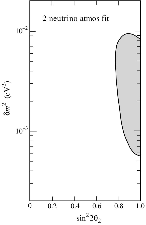
FIG. 1.: Allowed region at 95% C.L. for our effective two-neutrino fit to the Super-Kamiokande atmospheric neutrino data.

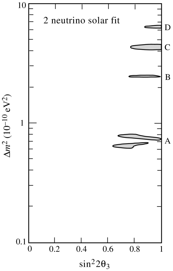
FIG. 2.: Allowed regions at 95% C.L. for our effective two-neutrino fit to the solar neutrino data from Homestake, SAGE, GALLEX, and Super-Kamiokande. The four “finger” regions from Table II are labeled A, B, C, and D.

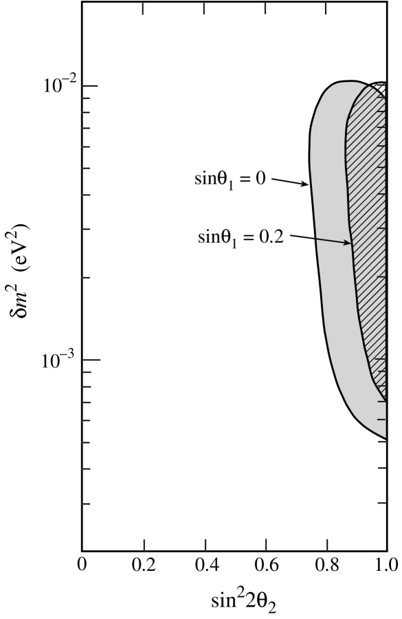
FIG. 3.: Allowed regions at 95% C.L. from the Super-Kamiokande atmospheric neutrino data for $\delta m^{2}_{atm}$ versus $\sin^{2}2\theta_{2}$ when the overall atmospheric neutrino flux normalization $\alpha$ is allowed to vary, for $\sin\theta_{1}=0$ and $\sin\theta_{1}=0.2$.

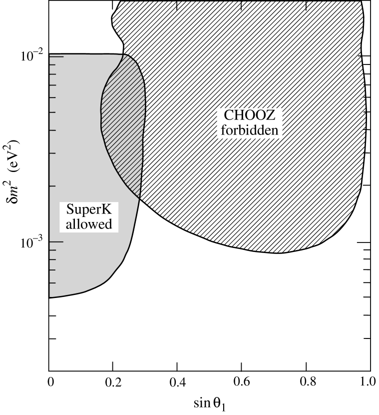
FIG. 4.: Allowed regions at 95% C.L. from the Super-Kamiokande atmospheric neutrino data for $\delta m^{2}_{atm}$ versus $\sin\theta_{1}$ when $\sin^{2}2\theta_{2}$ and the overall atmospheric neutrino flux normalization $\alpha$ are allowed to vary. The CHOOZ constraint is also shown.

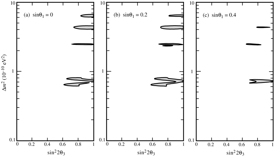
FIG. 5.: Allowed regions at 95% C.L. from the solar neutrino data for $\delta m^{2}_{sun}$ versus $\sin^{2}2\theta_{3}$ when the ⁸B neutrino flux normalization $\beta$ is allowed to vary, for (a) $\sin\theta_{1}=0$, (b) $\sin\theta_{1}=0.2$, and (c) $\sin\theta_{1}=0.4$

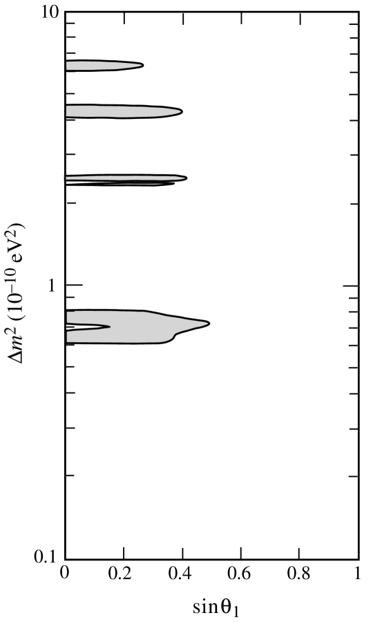
FIG. 6.: Allowed regions at 95% C.L. from the solar neutrino data for $\delta m^{2}_{sun}$ versus $\sin\theta_{1}$ when $\sin^{2}2\theta_{3}$ and the ⁸B neutrino flux normalization $\beta$ are allowed to vary.

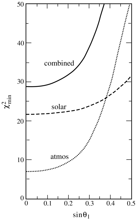
FIG. 7.: Minimum $\chi^{2}$ versus $\sin\theta_{1}$ for the atmsopheric data set (dotted line), the solar data set (dashed), and the combined atmospheric and solar data sets (solid). All other relevant parameters are allowed to vary in these fits.

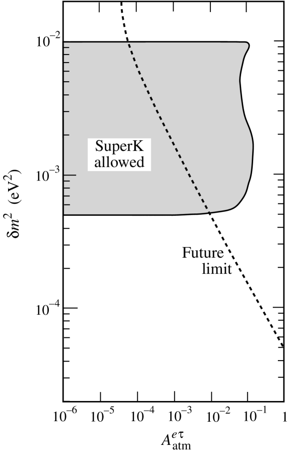
FIG. 8.: Allowed region at 95% C.L. of the $\nu_{e}\rightarrow\nu_{\tau}$ oscillation amplitude in atmospheric and long-baseline experiments versus $\delta m^{2}_{atm}$, determined from a fit to the atmospheric neutrino data set when the CHOOZ constraint is included. The expected sensitivity of a long-baseline experiment from Fermilab to Soudan using muon storage rings is shown by the dashed line.

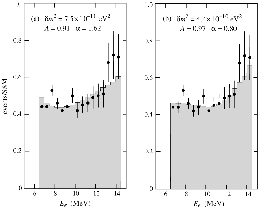
FIG. 9.: Ratio of the electron energy spectrum to the SSM prediction for two different two-neutrino vacuum long-wavelength oscillation scenarios, compared to the Super-Kamiokande data. The shaded histograms show the results when oscillations are included. The two cases shown are (a) the best overall fit to all solar neutrino data, solution A from Table II, and (b) the best fit to just the Super-Kamiokande data, solution C from Table II.

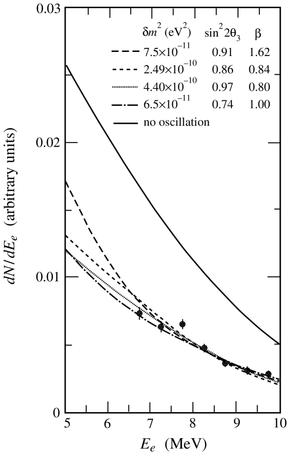
FIG. 10.: Electron energy spectrum in Super-Kamiokande for the Standard Solar Model with no oscillations (solid curve) and for the four vacuum neutrino oscillation solutions A (long-dashed), B (short-dashed), C (dotted), and D (dash-dotted) listed in Table II. Also shown is the current data from Super-Kamiokande [1].

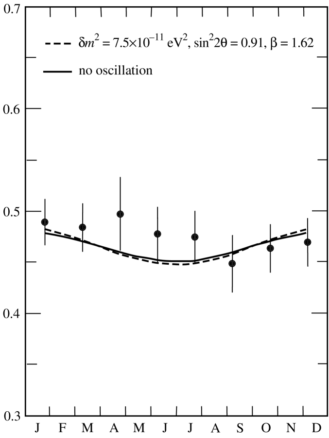
FIG. 11.: Predicted event rate as a fraction of the SSM value in Super-Kamiokande versus time of the year for vacuum oscillation Solution A in Table II (dashed curve) and for no oscillations when the overall event rate is normalized to the observed value (solid). The other solutions in Table II give similar results. Also shown is the current data from Super-Kamiokande [1].

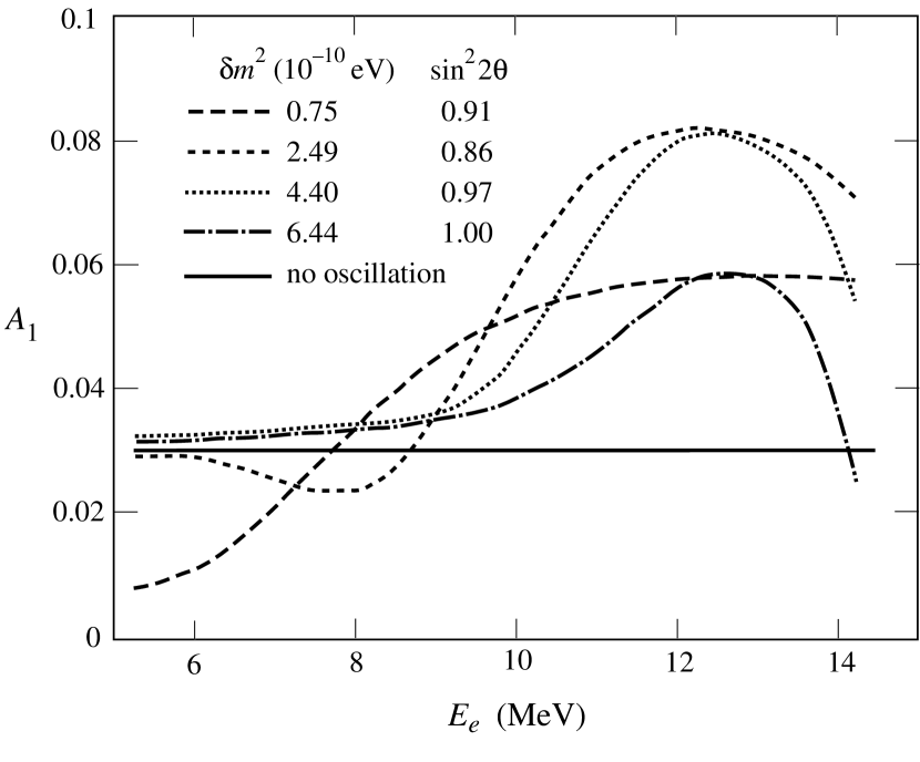
FIG. 12.: Predicted values for the seasonal asymmetry $A_{1}$ defined in Eq. (54) versus electron energy in the SuperK experiment for the four vacuum neutrino oscillation solutions A (long-dashed curve), B (short-dashed), C (dotted), and D (dash-dotted) listed in Table II. Also shown is the energy-independent value for no oscillations (solid).

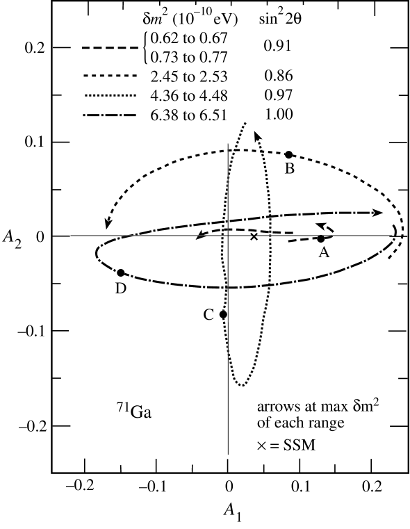
FIG. 13.: Typical predicted seasonal asymmetries $A_{2}$ versus $A_{1}$ (defined in Eqs. (54) and (55)) in the GALLEX and SAGE experiments for solutions from the four “finger” regions of Fig. 2: (a) $\sin^{2}2\theta_{3}=0.74$, $\delta m^{2}_{sun}=(0.62-0.67)\times 10^{-10}$ eV² and $\sin^{2}2\theta_{3}=0.91$, $\delta m^{2}_{sun}=(0.73-0.77)\times 10^{-10}$ eV² (long-dashed curves), (b) $\sin^{2}2\theta_{3}=0.86$, $\delta m^{2}_{sun}=(2.45-2.53)\times 10^{-10}$ eV² (short-dashed), (c) $\sin^{2}2\theta_{3}=0.97$, $\delta m^{2}_{sun}=(4.36-4.49)\times 10^{-10}$ eV² (dotted), and (d) $\sin^{2}2\theta_{3}=1.00$, $\delta m^{2}_{sun}=(6.38-6.51)\times 10^{-10}$ eV² (dash-dotted). The predictions of best-fit solutions A, B, C, D from Table II are indicated by the solid circles. In cases (c) and (d), $\delta m^{2}_{sun}$ can vary over a wider range than shown; the additional values give orbits in $A_{1}$–$A_{2}$ space that are slightly shifted from those shown here. The arrow on each curve is at the maximum value of $\delta m^{2}_{sun}$ for each range. The no oscillation prediction (where the only variation in signal comes from the variation of the flux due to the elliptical orbit) is shown by a cross.

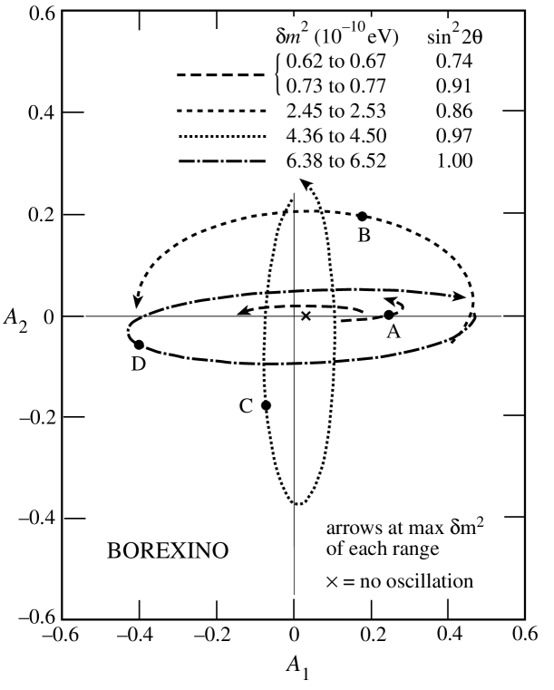
FIG. 14.: Same as Fig. 13 for the BOREXINO experiment. Cross sections have been calculated for final-state electron kinetic energies in the range $0.26{\rm~{}MeV}\leq T_{e}\leq 0.665$ MeV.

REFERENCES

- [1] Super-Kamiokande Collaboration, talk by Y. Suzuki at Neutrino-98, Takayama, Japan, June 1998.
- [2] Super-Kamiokande Collaboration, Y. Fukuda et al., Phys. Lett. B433, 9 (1998); Phys. Lett. B436, 33 (1998); Phys. Rev. Lett. 81, 1562 (1998).
- [3] B.T. Cleveland et al., Nucl. Phys. B (Proc. Suppl.) 38, 47 (1995).
- [4] Kamiokande collaboration, Y. Fukuda et al., Phys. Rev. Lett, 77, 1683 (1996).
- [5] GALLEX Collaboration, W. Hampel et al., Phys. Lett. B388, 384 (1996); SAGE collaboration, J.N. Abdurashitov et al., Phys. Rev. Lett. 77, 4708 (1996).
- [6] J.N. Bahcall and R.K. Ulrich, Rev. Mod. Phys. 60, 297 (1988).
- [7] J.N. Bahcall, S. Basu, and M.H. Pinsonneault, Phys. Lett. B433, 1 (1998).
- [8] J.G. Learned, S. Pakvasa, and T.J. Weiler, Phys. Lett. B207, 79 (1988); V. Barger and K. Whisnant, Phys. Lett. B209, 365 (1988); K. Hidaka, M. Honda, and S. Midorikawa, Phys. Rev. Lett. 61, 1537 (1988).
- [9] Kamiokande collaboration, K.S. Hirata et al., Phys. Lett. B280, 146 (1992); Y. Fukuda et al., Phys. Lett. B335, 237 (1994); IMB collaboration, R. Becker-Szendy et al., Nucl. Phys. Proc. Suppl. 38B, 331 (1995); Soudan-2 collaboration, W.W.M. Allison et al., Phys. Lett. B391, 491 (1997).
- [10] Liquid Scintillator Neutrino Detector (LSND) collaboration, C. Athanassopoulos et al., Phys. Rev. Lett. 75, 2650 (1995); ibid. 77, 3082 (1996); ibid. 81, 1774 (1998); talk by H. White at Neutrino-98, Takayama, Japan, June 1998.
- [11] KARMEN collaboration, K. Eitel and B. Zeitnitz, at Neutrino-98, Takayama, Japan, June 1998, hep-ex/9809007; future tests of the LSND results will be made by the KARMEN experiment and also by the mini-BooNE experiment, E. Church et al., nucl-ex/9706011; see also J.M. Conrad, talk at ICHEP-98, hep-ex/9811009
- [12] J.W. Flanagan, J.G. Learned, and S. Pakvasa, Phys. Rev. D57, 2649 (1998); M.C. Gonzalez-Garcia, H. Nunokawa, O. Peres, T. Stanev, and J.W.F. Valle, Phys. Rev. D58, 033004 (1998); M.C. Gonzalez-Garcia, H. Nunokawa, O. Peres, and J.W.F. Valle, hep-ph/9807305; C.H. Albright, K.S. Babu, and S.M. Barr, Phys. Rev. Lett. 81, 1167 (1998).; J. Bordes, H.-M. Chan, J. Pfaudler, and S.T. Tsou, Phys. Rev. D58, 053003 (1998); J.G. Learned, S. Pakvasa, and J.L. Stone, Phys. Lett. B435, 131 (1998); L.J. Hall and H. Murayama, Phys. Lett. B436, 323 (1998); S.F. King, hep-ph/9806440.
- [13] M. Drees, S. Pakvasa, X. Tata, and T. ter Veldhuis, Phys. Rev. D57, 5335 (1998); E.J. Chun, S.K. Kang, C.W. Kim, and U.W. Lee, hep-ph/9807327; V. Bednyakov, A. Faessler, and S. Kovalenko, hep-ph/9808224; B. Mukhopadhaya, S. Roy, and F. Vissani, hep-ph/9808265; O.C.W. Kong, hep-ph/98084304; E.J. Chun and J.S. Lee, hep-ph/9811201; L. Clavelli and P.H. Frampton, hep-ph/9811326; Z. Berezhiani and A. Rossi, hep-ph/9811447.
- [14] V. Barger, S. Pakvasa, T.J. Weiler, and K. Whisnant, Phys. Lett. B437 107 (1998); A.J. Baltz, A.S. Goldhaber, and M. Goldhaber, hep-ph/9806540; M. Jezabek and Y. Sumino, hep-ph/9807310; Y. Nomura and T. Yanagida, hep-ph/9807325; G. Altarelli and F. Feruglio, Phys. Lett. B439, 112 (1998); hep-ph/9809596; H. Georgi and S. Glashow, hep-ph/9808293; S. Davidson and S.F. King, hep-ph/9808296. R.N. Mohapatra and S. Nussinov, hep-ph/9808301; hep-ph/9809415; S.K. Kang and C.S. Kim, hep-ph/9811379.
- [15] H. Fritzsch and Z. Xing, Phys. Lett. B372, 265 (1996); hep-ph/9807234; hep-ph/9808272; E. Torrente-Lujan, Phys. Lett. B389, 557 (1996); M. Fukugita, M. Tanimoto, and T. Yanagida, Phys. Rev. D57, 4429 (1998); M. Tanimoto, hep-ph/9807283.
- [16] R. Barbieri, L.J. Hall, D. Smith, A. Strumia, and N. Weiner, hep-ph/9807235; R. Barbieri, L.J. Hall, and A. Strumia, hep-ph/9808333.
- [17] E. Ma, hep-ph/9807386; J. Ellis, G.K. Leontaris, S. Lola, and D.V. Nanopoulos, hep-ph/9808251; S. Lola and J.D. Vergados, hep-ph/9808269; K. Kang, S.K. Kang, C.S. Kim, and S.M. Kim, hep-ph/9808419; E. Ma, D.P. Roy, and U. Sarkar, hep-ph/9810309; E. Malkawi, hep-ph/9810542; E. Ma and D.P. Roy, hep-ph/9811266; J. Elwood, N. Irges, and P. Ramond, hep-ph/9807228.
- [18] Analyses that have considered the both atmospheric and MSW solar oscillations include A. Joshipura and P. Krastev, Phys. Rev. D50, 3484 (1994), and the first paper of Ref [16].
- [19] V. Barger, R.J.N. Phillips, and K. Whisnant, Phys. Rev. D24, 538 (1981); S.L. Glashow and L.M. Krauss, Phys. Lett. B190, 199 (1987).
- [20] A. Acker, S. Pakvasa, and J. Pantaleone, Phys. Rev. D43, 1754 (1991); V. Barger, R.J.N. Phillips, and K. Whisnant, Phys. Rev. Lett. 69, 3135 (1992); P.I. Krastev and S.T. Petcov, Phys. Lett. B285, 85 (1992); Phys. Rev. Lett. 72, 1960 (1994); Phys. Rev. D53, 1665 (1996).
- [21] CHOOZ collaboration, M. Apollonio et al., Phys. Lett. B420, 397 (1998).
- [22] V. Barger, K. Whisnant, D. Cline, and R.J.N. Phillips, Phys. Lett. B93, 194 (1980).
- [23] V. Barger, T.J. Weiler, and K. Whisnant, hep-ph/9807319, Phys. Lett. B (in press).
- [24] C. Jarlskog, Z. Phys. C29, 491 (1985); Phys. Rev. D35, 1685 (1987).
- [25] See, for example, R.N. Mohapatra and P.B. Pal, Massive Neutrinos in Physics and Astrophysics (World Scientific, Singapore, 1991), p. 61-62.
- [26] See, e.g., the Particle Data Group’s 1998 Review of Particle Properties, C. Caso et al., Euro. Phys. J. 3, 1 (1998).
- [27] G. Barr, T.K. Gaisser, and T. Stanev, Phys. Rev. D39, 3532 (1989); M. Honda, T. Kajita, K. Kasahara, and S. Midorikawa, Phys. Rev. D52, 4985 (1995); V. Agrawal, T.K. Gaisser, P. Lipari, and T. Stanev, Phys. Rev. D53, 1314 (1996); T.K. Gaisser and T. Stanev, Phys. Rev. D57, 1977 (1998).
- [28] We use an updated version of the neutrino flux in the first paper of Ref. [27]; a program to calculate the flux was provided by T. Stanev.
- [29] See, e.g., V. Barger and R.J.N. Phillips, Collider Physics (Addison-Wesley, New York, updated edition, 1995), p.143.
- [30] R.H. Bernstein and S.J. Parke, Phys. Rev. D44, 2069 (1991); E.K. Akhmedov, P. Lipari, and M. Lusignoli, Phys. Lett. B300, 128 (1993); Q.Y. Liu and A. Yu. Smirnov, Nucl. Phys. B524, 505 (1998); Q.Y. Liu, S.P. Mikheyev, and A. Yu. Smirnov, hep-ph/9803415; S.T. Petcov, Phys. Lett. B434, 321 (1998); E.K. Akhmedov, hep-ph/9805272; E.K. Akhmedov, A. Dighe, P. Lipari, and A.Y. Smirnov, hep-ph/9808270; M. Chizhov, M. Maris, and S.T. Petcov, hep-ph/9810501.
- [31] J. Pantaleone, Phys. Rev. D49, 2152 (1994).
- [32] The effects of a nonzero on solar oscillation fits are considered by Z. Berezhiani and A. Rossi, Phys. Lett. B367, 219 (1996), P. Osland and G. Vigdel, Phys. Lett. B438, 129 (1998), and the first paper in Ref. [16].
- [33] S.M. Bilenky and C. Giunti, hep-ph/9802201.
- [34] T.K. Gaisser et al., Phys. Rev. D54, 5578 (1996).
- [35] J. Bahcall, P. Krastev, and A. Smirnov, Phys. Rev. D58, 096016 (1998); a comprehensive fit to earlier data was done by N. Hata and P. Langacker, Phys. Rev. 56, 6116 (1997).
- [36] A. Acker and S. Pakvasa, Phys. Lett. B397, 209 (1997); P.F. Harrison, D.H. Perkins and W.G. Scott, Phys. Lett. B396, 186 (1997); Phys. Lett. B349, 137 (1995); G. Conforto, A. Marchionni, F. Martelli, F. Vetrano, M. Lanfranchi and G. Torricelli-Ciamponi, Astrop. Physics 5, 147 (1996); G. Conforto, A. Marchionni, F. Martelli and F. Vetrano, Phys. Lett. B427, 314 (1998); G. Conforto, M. Barone and C. Grimani, hep-ph/9809501; R.P. Thun and S. McKee, Phys. Lett. B439, 123 (1998).
- [37] P.I. Krastev and S.T. Petcov, Phys. Lett. B395, 69 (1997); see also G. Conforto, C. Grimani, F. Martelli and F. Vetrano, hep-ph/9807306.
- [38] Three-parameter fits to older atmospheric data without explicit dependence were made by S.M. Bilenky, C. Giunti, and C.W. Kim, Astropart. Phys. 4, 241 (1996), using the ratio of muon to electron rates, and the first paper of Ref. [16], using up/down ratios; see also C. Giunti, C.W. Kim, and M. Monteno, Nucl. Phys. B521, 3 (1998); O. Yasuda, Phys. Rev. D58, 091301 (1998); hep-ph/9809205; G.L. Fogli, E. Lisi, A. Marrone, G. Scioscia, hep-ph/9808205.
- [39] MINOS Collaboration, “Neutrino Oscillation Physics at Fermilab: The NuMI-MINOS Project,” NuMI-L-375, May 1998.
- [40] K. Nishikawa, talk at Neutrino-98, Takayama, Japan, June 1998;
- [41] F. Pietropaola, talk at Neutrino-98, Takayama, Japan, June 1998;
- [42] S. Geer, Phys. Rev. D57, 6989 (1998).
- [43] V. Barger, K. Whisnant, and T.J. Weiler, Phys. Lett. B427, 97 (1998); V. Barger, S. Pakvasa, T.J. Weiler, and K. Whisnant, Phys. Rev. D58, 093016 (1998).
- [44] A. De Rujula, M.B. Gavela, and P. Hernandez, hep-ph/9811390.
- [45] R. Escribano, J.M. Frere, A.Gevaert, and D. Monderen, Phys. Lett. B444, 397 (1998); J.N. Bahcall and P. Krastev, Phys. Lett. B436, 243 (1998).
- [46] SNO Collaboration, E. Norman et al., in proc. of The Fermilab Conference: DPF 92, November 1992, Batavia, IL, ed. by C. H. Albright, P.H. Kasper, R. Raja, and J. Yoh (World Scientific, Singapore, 1993), p. 1450.
- [47] V. Barger, R.J.N. Phillips, and K. Whisnant, Phys. Rev. Lett. 65, 3084 (1990); S. Pakvasa and J. Pantaleone, Phys. Rev. Lett. 65, 2479 (1990); A. Acker, Ph.D. thesis, Dec. 1992, UH-511-759-92.
- [48] For recent discussions, see B. Faid, G.L. Fogli, E. Lisi, and D. Montanino, hep-ph/9805293; V. Berezinsky, G. Fiorentini, and M. Lissia, hep-ph/9811352; S.L. Glashow, P.J. Kernan, and L.M. Krauss, hep-ph/9808470.
- [49] S.P. Mikheyev and A.Yu. Smirnov, Phys. Lett. B429, 343 (1998).
- [50] V. Barger, R.J.N. Phillips, and K. Whisnant, Phys. Rev. D43, 1110 (1991).
- [51] J.M. Gelb and S.P. Rosen, hep-ph/9809508; see also the second paper of Ref. [48].
- [52] BOREXINO Collaboration, C. Arpesella et al., “INFN Borexino proposal,” Vols. I and II, edited by G. Bellini, R. Raghavan et al. (Univ. of Milan, 1992); J. Benziger, F.P. Calaprice et al., “Proposal for Participation in the Borexino Solar Neutrino Experiment,” (Princeton University, 1996).