INT #DOE/ER/40561-18-INT98

TRI-PP-98-26

Spectral Content of Isoscalar Nucleon Form Factors

H.-W. Hammer^a, and M.J. Ramsey-Musolf^b,c,

^a TRIUMF, 4004 Wesbrook Mall, Vancouver, BC, Canada V6T 2A3

^b Department of Physics, University of Connecticut, Storrs, CT 06269, USA

^c Institute for Nuclear Theory, University of Washington, Seattle, WA 98195, USA

The nucleon strange vector and isoscalar electromagnetic form factors are studied using a spectral decomposition. The $K\bar{K}$ contribution to the electric and magnetic radii as well as the magnetic moment is evaluated to all orders in the strong interaction using an analytic continuation of experimental $KN$ scattering amplitudes and bounds from unitarity. The relationship between non-resonant and resonant $K\bar{K}$ contributions to the form factors is demonstrated, and values for the vector and tensor $\phi N\bar{N}$ couplings are derived. The $K\bar{K}$ spectral functions are used to evaluate the credibility of model calculations for the strange quark vector current form factors.
PACS: 14.20.Dh, 11.55.Fv, 12.38.Lg, 14.65.Bt
Keywords: nucleon form factors; dispersion relations; strangeness

1 Introduction

The reasons for the success of the constituent quark model of light hadrons remains one of the on-going mysteries of strong interaction physics. Although deep inelastic scattering has provided incontrovertible evidence for the existence of gluons and QCD current quarks in the lightest hadrons, these degrees or freedom are manifestly absent from the the quark model. Nevertheless, a description of light hadrons solely in terms of constituent quarks moving in an effective potential has been enormously successful in accounting for the mass spectrum and other properties of low-lying hadrons. Various explanations for this situation have appeared in the literature, including the simple and intuitive idea that the sea quarks and gluons of QCD “renormalize” the valence current quarks into the constituent quarks of the quark model [1]. In this picture, for example, the multitude of QCD degrees of freedom appear to a long wavelength probe primarily as single objects carrying the quantum numbers and effective mass of the constituent quark. From the standpoint of the quark-quark effective potential, gluon and sea-quarks are similarly un-discernible – as they help renormalize the quark model string tension into the physical value used as model input [2]. In fact, most low-energy observables studied to date are unable to uncover explicit signatures of QCD degrees of freedom.

There have been, however, a few exceptions to this situation. Of particular interest are observables sensitive to the presence of strange quarks in the nucleon. In contrast to up- and down-quarks, which appear both as valence and sea quarks, strange quarks constitute a purely sea-quark degree of freedom. Being the lightest such objects, they ought to generate the largest effects (in comparison to the heavier quarks). Consequently, nucleon matrix elements of strange quark operators provide an interesting window on the $q\bar{q}$ sea and as such may shed new light on the connection between non-perturbative QCD and the quark model. Indeed, were strange-quark observables found to be vanishingly small, one might ascribe the quark model’s success partly to the numerical insignificance of sea quark effects. In fact, the situation is more ambiguous. As is well-known, analyses of the “$\sigma$-term” in $\pi N$ scattering, the $g_{1}$ sum in polarized deep inelastic scattering, and $\nu_{\mu}\ (\bar{\nu}_{\mu})\ N$ deep inelastic scattering suggest that non-trivial fractions of the nucleon mass, spin, and light-cone momentum arise from the $s\bar{s}$ sea (see Ref. [3] and references therein). Evidently, the most naïve explanation for the quark model’s validity is ruled out by these analyses.

More recently, a well-defined program has begun to determine the matrix element ${\langle N|}{\bar{s}}\gamma_{\mu}s{|N\rangle}$ using parity-violating elastic and quasi-elastic electron scattering from the proton and nuclei [3]. The first result for the magnetic form factor associated with this matrix element has been reported by the SAMPLE collaboration at MIT-Bates [4]:

$${G_{{\scriptscriptstyle M}}^{s}}(q^{2}=-0.1\mbox{ GeV}^{2})=0.23\pm 0.37\pm 0.15\pm 0.19\,,$$ (1)

where $q^{2}$ is the four-momentum transfer squared. (The first error is statistical, the second is the estimated systematic error, and the last uncertainty is due to radiative corrections entering the analysis.) Although the value is consistent with zero, the error bars are large. Improved accuracy is expected when the full data set is analyzed. Similarly, a combination of the strange magnetic and electric form factors have been determined by the HAPPEX collaboration[5]:

$${G_{{\scriptscriptstyle E}}^{s}}+0.39{G_{{\scriptscriptstyle M}}^{s}}(q^{2}=-0.48\mbox{ GeV}^{2})=0.023\pm 0.034\pm 0.022\pm 0.026\,,$$ (2)

where the first two errors are again of statistical and systematic origin, respectively, and the last one arises from the estimated uncertainty in the electric neutron form factor. While no definitive conclusion can as yet be made regarding the experimental scale of ${\langle N|}{\bar{s}}\gamma_{\mu}s{|N\rangle}$, one expects to be able to do so at the conclusion of the measurements.

In contrast, the theoretical understanding of ${\langle N|}{\bar{s}}\gamma_{\mu}s{|N\rangle}$ is much less clear. The difficulty lies with the mass scales relevant to strange quark dynamics. In contrast to the heavy quarks, for which $m_{q}\gg\Lambda_{QCD}$, the strange quark has $m_{s}\sim\Lambda_{QCD}$. Consequently, the lifetime of a virtual $s{\bar{s}}$ pair is commensurate with typical strong interaction timescales, allowing the pair to exchange a plethora of gluons with other quarks and gluons in its environment. The dynamics of the pair are therefore inherently non-perturbative. Given the present state of QCD theory, a complete, first principles treatment of ${\langle N|}{\bar{s}}\gamma_{\mu}s{|N\rangle}$ has remained beyond reach. Attempts to obtain this matrix element on the lattice have produced two results for ${G_{{\scriptscriptstyle M}}^{s}}(q^{2}=0)$, neither of which agree with each other nor with the first SAMPLE results [6, 7], and one result for the slope of ${G_{{\scriptscriptstyle E}}^{s}}$ at the origin with large error bars [7].

An alternative – and more popular approach – has been to employ various effective frameworks, with varying degrees of model-dependence. These frameworks have included nucleon models, chiral perturbation theory (ChPT), and dispersion relations. Generally speaking, the degrees of freedom adopted in each of these approaches have been hadronic rather than quark and gluon, given that the lifetime of an $s{\bar{s}}$ pair permits it to form strange hadronic states. Apart from a few exceptions, effective approaches do not address the way in which QCD sea quarks hadronize. Hence, the connection with QCD is indirect at best, with each approach emphasizing some aspects of the strong interaction to the exclusion of others.

Not surprisingly, the range of predictions for the strangeness form factors is broad. In particular, the breadth of model predictions appears to be as wide as the variety of models that has been used even though the same models are in reasonable agreement for standard nucleon observables [3, 8, 9]. This situation illustrates the sensitivity of sea quark observables to model assumptions and the limited usefulness of models in making airtight predictions. One might have hoped for more insight from ChPT, which relies on the chiral symmetry of QCD to successfully account for a wide variety of other low-energy observables [10]. Unfortunately, ChPT is unable to make a prediction for the leading non-vanishing parts of ${G_{{\scriptscriptstyle M}}^{s}}$ or ${G_{{\scriptscriptstyle E}}^{s}}$ since the leading moments depend on unknown counterterms [11]. Recently, however, it has been noticed that slope of ${G_{{\scriptscriptstyle M}}^{s}}$ at the origin is independent of unknown counterterms to ${\cal O}(p^{3})$ [12].

In the present study, we turn to dispersion relations (DR’s) to derive insight into ${\langle N|}{\bar{s}}\gamma_{\mu}s{|N\rangle}$. Like ChPT, DR’s rely on certain general features of QCD (and other field theories) to relate existing experimental data to the observables of interest. In the case of DR’s it is analyticity and causality, rather than chiral symmetry, which allow one to make the connection. Although DR’s do not bear on the way in which QCD quarks and gluons form intermediate strange hadronic states, they do provide an essentially model-independent framework for treating the way in which those states contribute to the form factors. We view them as providing an intermediate step toward understanding the strange quark form factors at the fundamental level of QCD. Because of their generality, they also allow us to evaluate the credibility of several model predictions.

Our use of DR’s to study nucleon form factors is not new. The spectral content of the nucleon isovector form factors has been clearly delineated using this approach [13, 14]. It is now known that both an un-correlated $\pi\pi$ continuum as well as the $\pi\pi\to\rho$ resonance play important roles in the low-$q^{2}$ behavior of these form factors. The $q^{2}$-dependence of the isoscalar EM form factors has been successfully reproduced using DR’s under the assumption of vector meson dominance (VMD). The results have been used to infer relations between the $\omega NN$ and $\phi NN$ coupling strengths and to make predictions for the strange quark form factors [15, 16, 17]. However, the relationship between the resonance and continuum contributions to these form factors has not been previously established. Consequently, a number of model predictions have appeared which rely on the assumption that the uncorrelated continuum (“meson cloud”) gives the largest effect. These meson cloud calculations have generally entailed a truncation at second order in the strong hadronic coupling, $g$ – a practice of questionable validity. The corresponding predictions have generally been in disagreement with those obtained using VMD.

In what follows, we consider both the strange quark and isoscalar EM form factors without relying on the a priori assumption of vector meson or meson cloud dominance. We focus in particular on the contribution from the $K{\bar{K}}$ intermediate state. The rationale for this focus is twofold. First, the $K{\bar{K}}$ state constitutes the lightest intermediate state containing valence $s$ and ${\bar{s}}$ quarks. Its contribution to the strange quark form factors has correspondingly been emphasized in both models and ChPT. Second, given the present availability of strong interaction and EM data, the $K\bar{K}$ contribution can be computed to all orders in $g$ using a minimum of assumptions. From an analysis of $KN\to KN$ and $e^{+}e^{-}\to K{\bar{K}}$ data, we show that the scale of the $K{\bar{K}}$ contribution depends critically on effects going beyond ${\cal O}(g^{2})$ and argue that a similar situation holds for the remainder of the form factor spectral content. We also

(a) illustrate the relation between the continuum and resonance contributions,

(b) evaluate the credibility of several model predictions as well as the ${\cal O}(p^{3})$ prediction of ChPT for the magnetic radius,

(c) derive values for the vector and tensor $\phi NN$ couplings and compare with those obtained from isoscalar EM form factors under the assumption of VMD.

In Refs. [18, 19], we reported on the results of our DR analysis of the $K\bar{K}$ contribution to the nucleon “strangeness radius” (the slope of ${G_{{\scriptscriptstyle E}}^{s}}$ at the photon point). Here, we expand on that analysis to consider the full $q^{2}$-dependence in both the isoscalar EM and strangeness channels and to discuss both the electric and magnetic form factors. Since the DR approach requires knowledge of the $K{\bar{K}}\to N{\bar{N}}$ amplitudes in the unphysical region, some form of analytic continuation is needed to complete the analysis. Using backward dispersion relations, we obtain the unphysical amplitudes from $KN$ phase shift analyses. The results of this continuation and their implications for nucleon form factors constitute a central theme of this paper.

Our discussion of these issues is organized as follows. After outlining our formalism, we perform the spectral decomposition of the form factors and write down DR’s in Section 2. In Section 3, we express the spectral functions in terms of $K\bar{K}\to N\bar{N}$ partial waves and give the corresponding unitarity bounds valid in the physical region of the dispersion integrals. The analytic continuation of $KN$ amplitudes which is used in the unphysical region is performed in Section 4. A brief description of the analytic continuation and our treatment of the inherent problems is given. The results are applied to the nucleon’s strange and isoscalar EM form factors in Section 5. In Section 6, we discuss the contribution of other intermediate states and summarize our conclusions.

2 Spectral Decomposition and Dispersion Relations

The vector current form factors of the nucleon, $F_{1}(t)$ and $F_{2}(t)$, are defined by

$${\langle N(p^{\prime})|}j_{\mu}(0){|N(p)\rangle}=\bar{u}(p^{\prime})\left[F_{1}(t)\gamma_{\mu}+{iF_{2}(t)\over 2{m_{{\scriptscriptstyle N}}}}\sigma_{\mu\nu}(p^{\prime}-p)^{\nu}\right]u(p)\,.$$ (3)

where $t=q^{2}=(p^{\prime}-p)^{2}$. We consider two cases for $j_{\mu}$: (i) the strange vector current $\bar{s}\gamma_{\mu}s$ and (ii) the isoscalar EM current $j_{\mu}^{\scriptscriptstyle(I=0)}$. Since the nucleon carries no net strangeness, ${F_{1}^{s}}$ must vanish at zero momentum transfer, (i.e. ${F_{1}^{s}}(0)=0$), whereas ${F_{1}^{\scriptscriptstyle(I=0)}}$ is normalized to the isoscalar EM charge of the nucleon, ${F_{1}^{\scriptscriptstyle(I=0)}}(0)=1/2$. We also define the electric and magnetic Sachs form factors, which may be interpreted as the fourier transforms of the charge and magnetic moment distributions in the Breit frame,

$${G_{{\scriptscriptstyle E}}}={F_{1}}-\tau{F_{2}}\,,\qquad\qquad\qquad{G_{{\scriptscriptstyle M}}}={F_{1}}+{F_{2}}\,,$$ (4)

with $\tau=-t/4{m^{2}_{{\scriptscriptstyle N}}}$. In the case of the strange form factors we are particularly interested in their leading moments, the strange magnetic moment and the strange radii:

$$\kappa^{s}={F_{2}^{s}}(0)={G_{{\scriptscriptstyle M}}^{s}}(0)=\mu^{s}\,,\vphantom{\frac{1}{2}}$$ (5)

$$\langle r^{2}\rangle^{s}_{i}=6{d{G_{{\scriptscriptstyle i}}^{s}}(t)\over dt}\bigg{|}_{t=0}\,,$$

where $i=E,M$, respectively. A dimensionless version of the radii can be defined by

$$\rho^{s}_{E} = {d{G_{{\scriptscriptstyle E}}^{s}}(\tau)\over d\tau}\bigg{|}_{\tau=0}=-\frac{2}{3}{m^{2}_{{\scriptscriptstyle N}}}\langle r^{2}\rangle^{s}_{E}$$ (6)

and similarly for $\rho^{s}_{M}$. The leading moments of the EM form factors are defined analogously.

It is conventional to employ a once subtracted DR for $F_{1}$. Typically, one wishes to predict $F_{2}(0)$ as well as its $t\not=0$ behavior. In this case, an unsubtracted DR is appropriate. We follow this ansatz in the present study and obtain

$${F_{2}^{s}}(t)=\frac{1}{\pi}\int_{t_{\lambda}}^{\infty}\frac{\mbox{\sl{Im}}\,{F_{2}^{s}}(t^{\prime})}{t^{\prime}-t}dt^{\prime}\,,$$ (7)

and

$${F_{1}^{s}}(t)=\frac{t}{\pi}\int_{t_{\lambda}}^{\infty}\frac{\mbox{\sl{Im}}\,{F_{1}^{s}}(t^{\prime})}{t^{\prime}(t^{\prime}-t)}dt^{\prime}\,.$$ (8)

As a consequence, subtracted DR’s can be written for the Sachs form factors as well.

From Eqs. (7-8), it is clear that the quantities of interest are the imaginary parts of the form factors. The success of the DR analysis relies on a decomposition of the ${\mbox{\sl{Im}}\,F_{i}}$ into scattering amplitudes involving physical states. To obtain this spectral decomposition, we follow the treatment of Refs. [20, 21, 18] and consider the crossed matrix element

$$J_{\mu}={\langle N(p)\,\bar{N}(\bar{p})|}j_{\mu}(0){|0\rangle}=\bar{u}(p)\left[F_{1}(t)\gamma_{\mu}+{iF_{2}(t)\over 2{m_{{\scriptscriptstyle N}}}}\sigma_{\mu\nu}(\bar{p}+p)^{\nu}\right]v(\bar{p})\,,$$ (9)

where $t$ is now timelike. Using the LSZ reduction formalism and inserting a complete set of intermediate states, $\mbox{\sl{Im}}\,J_{\mu}$ may be expressed as

$$\mbox{\sl{Im}}\,J_{\mu} = \frac{\pi}{\sqrt{Z}}(2\pi)^{3/2}{\cal N}\sum_{\lambda}{\langle N(p)|}\bar{J_{N}}(0){|\lambda\rangle}{\langle\lambda|}j_{\mu}(0){|0\rangle}\,v(\bar{p})\,\delta^{4}(p+\bar{p}-p_{\lambda})\,,$$ (10)

where ${\cal N}$ is a spinor normalization factor and $J_{N}(0)$ a nucleon source. Eq. (10) determines the singularity structure of the form factors and relates their imaginary parts to on-shell matrix elements for other processes. The form factors have multiple cuts on the positive real $t$-axis. The invariant mass-squared $M_{\lambda}^{2}$ of the lightest state appearing in the sum defines the beginning of the first cut and the lower limit in the dispersion integrals: $M_{\lambda}^{2}=t_{\lambda}$. Since Eq. (10) is linear, the contributions of different ${|\lambda\rangle}$ can be treated separately.

There is an infinite number of contributing intermediate states ${|\lambda\rangle}$ which are restricted by the quantum numbers of the currents $\bar{s}\gamma_{\mu}s$ and $j_{\mu}^{\scriptscriptstyle(I=0)}$ $[I^{G}(J^{PC})=0^{-}(1^{--})]$. Naïvely, the lightest states generate the most important contributions to the leading moments of the current. Moreover, because of the source $J_{N}(0)$, the intermediate states must have zero baryon number. The lowest allowed states together with their thresholds are collected in Table 1. Resonances, such as the $\omega$, do not correspond to asymptotic states and are already included in the continuum contributions, such as that from the $3\pi$ state.

mesonic states	$t_{\lambda}[\,\mbox{GeV}^{2}]$	baryonic states	$t_{\lambda}[\,\mbox{GeV}^{2}]\vphantom{\Large[}$
$3\pi$	0.18	$N\bar{N}$	3.53
$5\pi$	0.49	$N\bar{N}\pi\pi$	4.67
$7\pi$	0.96	$\Lambda\bar{\Lambda}$	4.84
$K\bar{K}$	0.98	$\Sigma\bar{\Sigma}$	5.76
$K\bar{K}\pi$	1.28	$\Lambda\bar{\Sigma}\pi$	5.95
$\vdots$		$\vdots$

Table 1: Lowest mass intermediate states contributing to Eq. (10).

When sufficient data exist, experimental information may be used to determine the matrix elements appearing in Eq. (10). However, when the threshold $t_{\lambda}$ of the intermediate state ${|\lambda\rangle}$ is below the two-nucleon threshold, the values of the matrix element ${\langle N(p)|}\bar{J_{N}}(0){|\lambda\rangle}\,v(\bar{p})$ are also required in the unphysical region $t_{\lambda}\leq t\leq 4\,{m^{2}_{{\scriptscriptstyle N}}}$. In this case, the amplitude must be analytically continued from the physical to the unphysical regime. The first cut in the complex $t$-plane appears at the $3\pi$ production threshold, $t=9m_{\pi}^{2}$, and higher-mass intermediate states generate additional cuts. For example for ${|\lambda\rangle}={|K\bar{K}\rangle}$ the cut runs from $t=4{m_{{\scriptscriptstyle K}}^{2}}$ to infinity. Therefore, the matrix element for $K\bar{K}\longrightarrow\bar{N}N$ is also needed in the unphysical region $4{m_{{\scriptscriptstyle K}}^{2}}\leq t\leq 4{m^{2}_{{\scriptscriptstyle N}}}$, which requires an analytic continuation.

Some of the predictions for the ${F_{i}^{s}}$ reported in the literature are based on approximations to the spectral functions appearing in Eqs. (7, 8). The work of Refs. [15, 16, 17] employed a VMD approximation, which amounts to writing the spectral function as $\mbox{\sl{Im}}\,{F_{i}^{s}}(t)=\pi\sum_{j}a_{j}\delta(t-m_{j}^{2})$, where “$j$” denotes a particular vector meson resonance (e.g. $\omega$ or $\phi$) and the sum runs over a finite number of resonances. In terms of the formalism from above this approximation omits any explicit multi-meson intermediate states ${|n\rangle}$ and assumes that the products ${\langle N(p)|}\bar{J_{N}}(0){|\lambda\rangle}{\langle\lambda|}\bar{s}\gamma_{\mu}s{|0\rangle}v({\bar{p}})$ are strongly peaked near the vector meson masses. The same has been made conventional analyses of the isoscalar EM form factors [13, 14].

In contrast, a variety of hadronic effective theory and model calculations for the strange form factors have focused on contributions from the two-kaon intermediate state [3, 8, 11]. Even though ${|K{\bar{K}}\rangle}$ is not the lightest state appearing in Table 1, it is the lightest state containing valence strange quarks. The rationale for focusing on the $\bar{K{\bar{K}}}$ contribution is based primarily on the intuition that such states ought to give larger contributions to the matrix element ${\langle\lambda|}\bar{s}\gamma_{\mu}s{|0\rangle}$ than purely pionic states with no valence $s$ or $\bar{s}$ quarks. In other words, the kaons represent the lightest contribution favored by the OZI rule. Typically, kaon-cloud predictions have been computed to ${\cal O}(g^{2})$ only. The results for for $\rho^{s}_{E}$ in particular are smaller in magnitude than the vector meson dominance predictions and have the opposite sign. In what follows, we illustrate how both the structure and magnitude of the full kaon cloud contribution differ from the ${\cal O}(g^{2})$ result and how a $\phi$-resonance structure appears in the all-orders analysis.

Although we consider here only the $K{\bar{K}}$ intermediate state, we note in passing that the validity of this so called “kaon cloud dominance” ansatz is open to question for a variety reasons. As can be seen from Table 1, for example, the three-pion threshold is significantly below the $K\bar{K}$ threshold. Consequently, the $3\pi$ contribution is weighted more strongly in the dispersion integral than the $K\bar{K}$ contribution because of the denominators in Eqs. (7, 8). Moreover, three pions can resonate into a state having the same quantum numbers as the $\phi$ (nearly pure $s\bar{s}$), and thereby generate a non-trivial contribution to the current matrix element. Indeed, the $\phi$ has roughly a 15% branch to multi-pion final states (largely via a $\rho\pi$ resonance). Although such resonances do not appear explicitly in the sum over the states in Eq. (10), their impact nevertheless enters via the current matrix element ${\langle 3\pi|}\bar{s}\gamma_{\mu}s{|0\rangle}$ and the $N\bar{N}$ production amplitude ${\langle N(p)|}\bar{J_{N}}(0){|3\pi\rangle}v({\bar{p}})$. Thus, the $3\pi$ state could contribute appreciably to the strangeness form factors via its coupling to the $\phi$. We return to this possibility in Section 6 (see also Ref. [25]).

3 $K\bar{K}$ Intermediate State and Unitarity

In order to determine $K\bar{K}$ contribution to the spectral functions, we need the matrix elements ${\langle N(p)|}\bar{J_{N}}{|K(k)\bar{K}(\bar{k})\rangle}\,v(\bar{p})$ and ${\langle K(k)\bar{K}(\bar{k})|}j_{\mu}{|0\rangle}$. By expanding the $K\bar{K}\to N\bar{N}$ amplitude in partial waves, we are able to impose the constraints of unitarity in a straightforward way. In doing so, we follow the helicity amplitude formalism of Jacob and Wick [22]. With $\lambda$ and $\bar{\lambda}$ being the nucleon and antinucleon helicities, we write the corresponding $S$-matrix element as

$${\langle N(p,\lambda)\bar{N}({\bar{p}},\bar{\lambda})|}{\hat{S}}{|K(k)\bar{K}(\bar{k})\rangle}=$$ (11)

$$\hphantom{N(p,\lambda)}i(2\pi)^{4}\delta^{4}(p+{\bar{p}}-k-\bar{k})(2\pi)^{2}\left[{64t\over t-4m_{K}^{2}}\right]^{1/2}{\langle\theta,\phi,\lambda,\bar{\lambda}|}{\hat{S}}(P){|00\rangle}\,,$$

where $t=P^{2}=(p+{\bar{p}})^{2}$ and $m_{K}$ is the kaon mass. The matrix element ${\langle\theta,\phi,\lambda,\bar{\lambda}|}{\hat{S}}(P){|00\rangle}$ is then expanded in partial waves as [18, 22]

$$S_{\lambda,\bar{\lambda}}\equiv{\langle\theta,\phi,\lambda,\bar{\lambda}|}{\hat{S}}(P){|00\rangle}=\sum_{J}\left({2J+1\over 4\pi}\right)b_{J}^{\lambda,\bar{\lambda}}\;{\cal D}_{0\mu}^{J}(\phi,\theta,-\phi)^{\ast}\,,$$ (12)

where ${\cal D}_{\nu\,\nu^{\prime}}^{J}(\alpha,\beta,\gamma)$ is a Wigner rotation matrix with $\mu=\lambda-\bar{\lambda}$. The $b_{J}^{\lambda\,\bar{\lambda}}$ define partial waves of angular momentum $J$. Because of the quantum numbers of the isoscalar EM and strange vector currents, only the $J=1$ partial waves contribute to the spectral functions. Moreover, because of parity invariance only two of the four partial waves are independent. We choose ${b_{1}^{1/2,\,1/2}}$ and ${b_{1}^{1/2,\,-1/2}}$ which fulfill the threshold relation [18]

$$\left.{b_{1}^{1/2,\,-1/2}}(t)\right|_{t=4{m^{2}_{{\scriptscriptstyle N}}}}=\sqrt{2}\,\left.{b_{1}^{1/2,\,1/2}}(t)\right|_{t=4{m^{2}_{{\scriptscriptstyle N}}}}\,.$$ (13)

Using the above definitions, the unitarity of the $S$-matrix, $S^{{\dagger}}S=1$, requires that

$$|b_{J}^{\lambda,\bar{\lambda}}(t)|\leq 1\,,$$ (14)

for $t\geq 4{m^{2}_{{\scriptscriptstyle N}}}$. Consequently, unitarity gives model-independent bounds on the contribution of the physical region ($t\geq 4{m^{2}_{{\scriptscriptstyle N}}}$) to the imaginary part. In the unphysical region ($4{m_{{\scriptscriptstyle K}}^{2}}\leq t\leq 4{m^{2}_{{\scriptscriptstyle N}}}$), however, the partial waves are not bounded by unitarity. Therefore, we must rely upon an analytic continuation of $KN$ scattering amplitudes. This procedure is discussed in the next section.

The second matrix element appearing in Eq. (10), ${\langle K(k)\bar{K}(\bar{k})|}j^{(a)}_{\mu}{|0\rangle}$, is parametrized by the kaon vector current form factor ${F_{{\scriptscriptstyle K}}^{a}}$:

$${\langle 0|}j_{\mu}^{(a)}{|K(k)\bar{K}(\bar{k})\rangle} = (k-\bar{k})_{\mu}{F_{{\scriptscriptstyle K}}^{a}}(t)\,,$$ (15)

where $a$ denotes $EM$ or $s$ and ${F_{{\scriptscriptstyle K}}^{a}}(0)$ gives the corresponding charge (e.g., ${F_{{\scriptscriptstyle K}}^{s}}(0)=-1$).

From Eq. (10), the spectral functions are related to the partial waves and the kaon strangeness form factor by,

$$\mbox{\sl{Im}}\,{F_{1}^{(a)}}(t) = \mbox{\sl{Re}}\,\left\{\left({{m_{{\scriptscriptstyle N}}}q_{t}\over 4p_{t}^{2}}\right)\left[{E\over\sqrt{2}{m_{{\scriptscriptstyle N}}}}{b_{1}^{1/2,\,-1/2}}(t)-{b_{1}^{1/2,\,1/2}}(t)\right]{F_{{\scriptscriptstyle K}}^{a}}(t)^{\ast}\right\}\,,$$ (16)

$$\mbox{\sl{Im}}\,{F_{2}^{(a)}}(t) = \mbox{\sl{Re}}\,\left\{\left({{m_{{\scriptscriptstyle N}}}q_{t}\over 4p_{t}^{2}}\right)\left[{b_{1}^{1/2,\,1/2}}(t)-{{m_{{\scriptscriptstyle N}}}\over\sqrt{2}E}{b_{1}^{1/2,\,-1/2}}(t)\right]{F_{{\scriptscriptstyle K}}^{a}}(t)^{\ast}\right\}\,,$$ (17)

where

$$p_{t}=\sqrt{t/4-{m^{2}_{{\scriptscriptstyle N}}}}\,,\qquad q_{t}=\sqrt{t/4-m_{K}^{2}}\,,\qquad\mbox{and}\qquad E=\sqrt{t}/2\,.$$ (18)

The corresponding spectral functions for the Sachs form factors follow from Eq. (4),

$$\mbox{\sl{Im}}\,{G_{\scriptscriptstyle E}^{(a)}}(t) = \mbox{\sl{Re}}\,\left\{\left({q_{t}\over 4{m_{{\scriptscriptstyle N}}}}\right){b_{1}^{1/2,\,1/2}}(t){F_{{\scriptscriptstyle K}}^{a}}(t)^{\ast}\right\}\,,$$ (19)

$$\mbox{\sl{Im}}\,{G_{\scriptscriptstyle M}^{(a)}}(t) = \mbox{\sl{Re}}\,\left\{\left({q_{t}\over 2\sqrt{2t}}\right){b_{1}^{1/2,\,-1/2}}(t){F_{{\scriptscriptstyle K}}^{a}}(t)^{\ast}\right\}\,.$$ (20)

On one hand, Eqs. (16-20) may be used to determine the spectral functions from experimental data. On the other hand, one can impose bounds on the imaginary parts in the physical region by using Eq. (14). Eqs. (16-20) involve expressions of the type

$$\mbox{\sl{Re}}\,\left\{{b_{1}^{1/2,\,\pm 1/2}}({F_{{\scriptscriptstyle K}}^{a}})^{\ast}\right\}=|{b_{1}^{1/2,\,\pm 1/2}}||{F_{{\scriptscriptstyle K}}^{a}}|\cos(\delta_{1}-\delta_{K})=|{b_{1}^{1/2,\,\pm 1/2}}||{F_{{\scriptscriptstyle K}}^{a}}|(1+\gamma_{K})\,,$$ (21)

where the phase correction $\gamma_{K}$ is defined by $\gamma_{K}\equiv\cos(\delta_{1}-\delta_{K})-1$, with $\delta_{1}$ and $\delta_{K}$ the complex phases of the ${b_{1}^{\lambda,\bar{\lambda}}}$ and form factor, respectively. The experimental information on $\gamma_{K}$ is incomplete. Since $|1+\gamma_{K}|\leq 1$, however, we can take $\gamma_{K}=0$ to obtain an upper bound on the spectral functions. In order to obtain finite bounds for the Dirac and Pauli form factors at the $N\bar{N}$ threshold, we build in the correct threshold relation for the ${b_{1}^{\lambda,\bar{\lambda}}}$, Eq. (13). This is necessary to cancel the $1/p_{t}^{2}$ factor in Eqs. (16, 17). Strictly speaking, the relation holds only for $t=4{m^{2}_{{\scriptscriptstyle N}}}$. For simplicity, however, we assume this relation to be valid for all momentum transfers, as e.g. holds in the tree approximation of perturbation theory. Consequently, we have

$$|\mbox{\sl{Im}}\,{F_{1}^{(a)}}(t)| \leq \frac{q_{t}}{2\sqrt{2}(\sqrt{t}+2{m_{{\scriptscriptstyle N}}})}|{F_{{\scriptscriptstyle K}}^{a}}(t)|\,,$$ (22)

$$|\mbox{\sl{Im}}\,{F_{2}^{(a)}}(t)| \leq \frac{{m_{{\scriptscriptstyle N}}}q_{t}}{\sqrt{2t}(\sqrt{t}+2{m_{{\scriptscriptstyle N}}})}|{F_{{\scriptscriptstyle K}}^{a}}(t)|\,.$$ (23)

The unitarity bounds for the Sachs form factors are obtained more straightforwardly by simply setting $|{b_{1}^{1/2,\,\pm 1/2}}(t)|\leq 1$ in Eqs. (19, 20).

3.1 Kaon Form Factors

The timelike EM kaon form factor, ${F_{{\scriptscriptstyle K}}^{{\scriptscriptstyle EM}}}(t)$, has been determined from $e^{+}e^{-}\to K\bar{K}$ cross sections. A striking feature of ${F_{{\scriptscriptstyle K}}^{{\scriptscriptstyle EM}}}$ observed in these studies is the pronounced peak for $t\approx m_{\phi}^{2}$ [23]. At higher values of $t$, oscillations at a much smaller scale are observed. A variety of analyses of ${F_{{\scriptscriptstyle K}}^{{\scriptscriptstyle EM}}}$ in this region have been performed [23, 24], and it is found that ${F_{{\scriptscriptstyle K}}^{{\scriptscriptstyle EM}}}$ is well-described by a VMD parametrization:

$${F_{{\scriptscriptstyle K}}^{{\scriptscriptstyle EM}}}(t)=\sum_{V}C_{V}{m_{V}^{2}\over m_{V}^{2}-t-im_{V}\Gamma_{V}f_{V}(t)}\,,$$ (24)

where the sum is over vector mesons of mass $m_{V}$ and width $\Gamma_{V}$ and where $f_{V}(t)$ is some specified function of $t$. We use $f_{V}(t)=t/m_{V}^{2}$ [24]. In nearly all analyses, one finds for the residues: $C_{\rho}\approx 1/2$, $C_{\omega}\approx 1/6$, and $C_{\phi}\approx 1/3$. These residues may alternately be described in terms of the $V\gamma$ and $VK\bar{K}$ couplings: $C_{V}=g_{VK\bar{K}}/f_{V}\,,$ where $f_{\rho}\approx 5.1$, $f_{\omega}\approx 17$, and $f_{\phi}\approx 13$. The strong couplings can be determined from $\Gamma(\phi\to K\bar{K})$ and SU(3) relations.

To obtain ${F_{{\scriptscriptstyle K}}^{s}}(t)$ we follow Refs. [15, 11, 25] and draw upon the known flavor content of the vector mesons. The $\rho$ does not contribute to isoscalar form factors. To the extent that (i) the $\omega$ and $\phi$ satisfy ideal mixing (${|\phi\rangle}=-{|s\bar{s}\rangle}$ and ${|\omega\rangle}={|u\bar{u}+d\bar{d}\rangle}/\sqrt{2}$) and (ii) the valence quarks determine the low-$t$ behavior of the matrix elements ${\langle 0|}J_{\mu}{|V\rangle}$ one expects ${\langle 0|}\bar{s}\gamma_{\mu}s{|\omega\rangle}=0$ and ${\langle 0|}\bar{s}\gamma_{\mu}s{|\phi\rangle}=-3{\langle 0|}J_{\mu}^{EM}{|\phi\rangle}$. It is straightforward to account for deviations from ideal mixing [15, 11, 25]:

$$C_{\omega}^{(s)}/C_{\omega} = -\sqrt{6}\left[{\sin\epsilon\over\sin(\epsilon+\theta_{0})}\right]\approx-0.2\,,$$ (25)

$$C_{\phi}^{(s)}/C_{\phi} = -\sqrt{6}\left[{\cos\epsilon\over\cos(\epsilon+\theta_{0})}\right]\approx-3\,,$$

where the $s$ superscript denotes the residue for the strangeness form factor, $\theta_{0}$ is the “magic” octet-singlet mixing angle giving rise to pure $u\bar{u}+d\bar{d}$ and $s\bar{s}$ states and $\epsilon$ deviations from ideal mixing. From Eqs. (24) and (25) we observe that the time-like kaon strangeness form factor is dominated by the $\phi(1020)$ resonance. We note that the flavor rotation of Eq. (25) only gives the relative size of the $\omega$ and $\phi$ contributions but does not lead to the correct normalization for ${F_{{\scriptscriptstyle K}}^{s}}$ at $t=0$ which must be enforced by hand.

Figure 1: Different model parametrizations for ${F_{{\scriptscriptstyle K}}^{s}}$. Full line shows simple VMD model with the $\phi$ only, dashed line shows the flavor rotated VMD model including the $\omega$ and $\phi$, and dash-dotted line shows GS parametrization. Dotted vertical line indicates $K\bar{K}$ threshold.

In Fig. 1 we plot ${F_{{\scriptscriptstyle K}}^{s}}$ as given by Eqs. (24) and (25) and compare it with a simple VMD model [18] and the Gounaris-Sakurai (GS) parametrization for $F_{\pi}$ [26] with all $\rho$ parameters replaced by the corresponding ones for the $\phi$. We observe that the GS and VMD forms reproduce the essential features of ${F_{{\scriptscriptstyle K}}^{s}}$ as determined from $e^{+}e^{-}$ data and standard flavor rotation arguments. Since ${F_{{\scriptscriptstyle K}}^{s}}$ is needed for $t\geq 4{m_{{\scriptscriptstyle K}}^{2}}$, the $\omega$-contribution which gives rise to the bump around $t\approx 0.6\mbox{ GeV}^{2}$ in Fig. 1 is negligible. In comparison to the strong $\phi$ peak, the small scale oscillations at higher-$t$ have a negligible impact as well. When computing the leading strangeness moments, we find less a than 10% variation in the results when any of these different parametrizations for ${F_{{\scriptscriptstyle K}}^{s}}$ is used. In short, any model parametrization of ${F_{{\scriptscriptstyle K}}^{s}}$ showing the peak at the $\phi$ mass and having the correct normalization, ${F_{{\scriptscriptstyle K}}^{s}}(0)=-1$, may be used for the purpose of studying nucleon strangeness. The pointlike approximation, ${F_{{\scriptscriptstyle K}}^{s}}=-1$, however, misses important resonance physics. Throughout the remainder of this work, we will use the GS parametrization.

4 Analytic Continuation

To obtain the ${b_{1}^{\lambda,\bar{\lambda}}}$ for $4{m_{{\scriptscriptstyle K}}^{2}}\leq t\leq 4{m^{2}_{{\scriptscriptstyle N}}}$ we analytically continue physical amplitudes into the unphysical regime. The analytic continuation (AC) of a finite set of experimental amplitudes with non-zero error is fraught with potential ambiguities. Indeed, AC in this case is inherently unstable, and analyticity alone has no predictive power. Additional information must be used in order to stabilize the problem, as we discuss below [27].

In order to illustrate these issues and the methods we adopt to resolve them, we first briefly review the kinematics of $KN$ scattering (cf. Ref. [28]). It is useful to consider the $s$-, $u$-, and $t$-channel reactions simultaneously,

(a) $$s \qquad K(q_{i})+N(p_{i})\rightarrow K(q_{f})+N(p_{f})\,,$$-channel:

(b) $$u \qquad\bar{K}(-q_{f})+N(p_{i})\rightarrow\bar{K}(-q_{i})+N(p_{f})\,,$$-channel:

(c) $$t \qquad\bar{K}(-q_{f})+K(q_{i})\rightarrow\bar{N}(-p_{i})+N(p_{f})\,,$$-channel:

where the four-momenta of the particles are given in parentheses. In this notation the crossing relations between the different channels are immediately transparent. The three processes can be described in terms of the usual Mandelstam variables

$$s = (p_{i}+q_{i})^{2}\,,\qquad u=(p_{i}-q_{f})^{2}\,,\qquad\mbox{and}\qquad t=(q_{i}-q_{f})^{2}\,.$$ (27)

The invariant matrix element for the $KN$ scattering process has the structure,

$${\cal M}=\bar{u}(p_{f})\left[A(s,t)+\frac{1}{2}(/\!\!\!q_{i}+/\!\!\!q_{f})B(s,t)\right]u(p_{i})\,,$$ (28)

and the isospin decomposition of the invariant amplitudes $A$ and $B$ reads

$$A(s,t) = A^{+}(s,t)+A^{-}(s,t)\left(\vec{\tau}_{N}\cdot\vec{\tau}_{K}\right)\,,$$ (29)

$$B(s,t) = B^{+}(s,t)+B^{-}(s,t)\left(\vec{\tau}_{N}\cdot\vec{\tau}_{K}\right)\,.$$

We also need the $\Lambda$ and $\Sigma$ pole contributions to $A^{(\pm)}$ and $B^{(\pm)}$ which are given by

$$A^{(\pm)}_{\rm pole}(s,u) = \sum_{Y=\Lambda,\Sigma}\frac{g_{\scriptscriptstyle KNY}^{2}}{2}(m_{\scriptscriptstyle Y}-{m_{{\scriptscriptstyle N}}})\left(\frac{1}{u-m_{\scriptscriptstyle Y}^{2}}\pm\frac{1}{s-m_{\scriptscriptstyle Y}^{2}}\right)\,,$$ (30)

$$B^{(\pm)}_{\rm pole}(s,u) = \sum_{Y=\Lambda,\Sigma}\frac{g_{\scriptscriptstyle KNY}^{2}}{2}\left(\frac{1}{u-m_{\scriptscriptstyle Y}^{2}}\mp\frac{1}{s-m_{\scriptscriptstyle Y}^{2}}\right)\,.$$

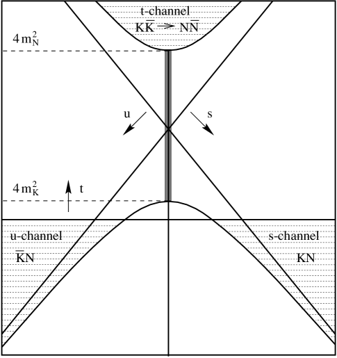
Figure 2: Mandelstam plane for $KN$ scattering. Physical regions are marked by dashed areas.

It is instructive to display the range of $s,u,$ and $t$ in the Mandelstam plane, shown in Fig 2. The physical regions of the three reactions do not overlap, and the invariant amplitudes simultaneously describe all three processes. The physical values of the invariant amplitudes are obtained when the Mandelstam variables are taken in the corresponding ranges. In order to carry out the dispersion integrals of Eqs. (7, 8), we require the ${b_{1}^{\lambda,\bar{\lambda}}}$ along the $t$-channel cut, indicated by the gray shaded area in Fig. 2.

We begin with experimental $KN$ amplitudes in the s-channel region and employ the method of backward DR to obtain the unphysical amplitudes along the $t$-channel cut. The backward DR method has has been used successfully for a similar continuation of $\pi N$ scattering amplitudes [29] and as a consistency test for different $KN$ phase shift solutions in the 1970’s [30]. Only recently has a continuation of the $KN$ amplitudes become possible due to improvements in the data base over the last three decades. A continuation of $KN$ scattering amplitudes has also been performed on the basis of hyperbolic DR [31]. In the latter analysis, however, the $t$-channel helicity amplitudes have been parametrized by sharp resonance poles, an a priori assumption we seek to avoid in the present analysis. We use the recent $KN$ phase shift analysis of the VPI-group [32] as experimental input.

4.1 Overall Strategy and Problems

Although an AC is uniquely defined from a continuum of points, this is not the case for a finite set of points lying within a certain error corridor. Consequently, the procedure for obtaining amplitudes outside the range of the given data is unstable. In practice the problem is stabilized by restricting the admissible solutions. This is achieved by using a priori information on the solution from experiment or theory as “stabilizing levers” [27]. In the remainder of this subsection, we give an overview of our general procedure for making this stabilized continuation [28, 19].

The first important observation is that in the backward direction, the invariant amplitudes in the $s$- and $t$-channel coincide, i.e. $f_{s}(t,\theta_{s}=\pi)=f_{t}(t,\theta_{t}=\pi)=f(t)$. Here $f$ is a generic invariant amplitude and $\theta_{s}$ and $\theta_{t}$ are the CM-scattering angles in the $s$- and $t$-channel, respectively. Thus, the continued amplitude $f_{s}(t,\theta_{s}=\pi)$ in the unphysical regime can be identified with the unphysical $t$-channel amplitude, $f_{t}(t,\theta_{t}=\pi)$.

Second, we work on a Riemann sheet where only the singularities from the $s$- and $t$-channel reactions are present. The backward amplitude $f$ then possesses a left-hand cut from zero to minus infinity stemming from the $s$-channel reaction. The lowest right-hand cut, which is due to the $3\pi$ intermediate state in the $t$-channel, runs from $9m_{\pi}^{2}$ to infinity. The two cuts do not overlap and we can write an unsubtracted DR for $f$. The amplitude is known from experiment on the left-hand cut in the region $t_{p}\leq t\leq 0$ and we need its values on the right-hand cut where $f$ is related to the $K\bar{K}\to N\bar{N}$ partial waves. In particular, we are interested in the unphysical region $4{m_{{\scriptscriptstyle K}}^{2}}\leq t\leq 4{m^{2}_{{\scriptscriptstyle N}}}$ where the partial waves are not bounded by unitarity.

Following our strategy to include as much a priori information as possible, we do not continue the amplitude $f$ itself but rather a related function, $\Delta f$, the so-called discrepancy function. In $\Delta f$ the analytically determined pole terms for $f$, as well as the experimentally known behavior of the amplitude, have been subtracted out. This subtraction is carried out in such a way as to remove the portion of the left-hand cut lying in the range $t_{p}\leq t\leq 0$ where the phase shift analyses are available. Thus, the use of $\Delta f$ presents two advantages. First, the original problem which entailed an AC from the boundary of the region of analyticity to another point on the boundary ($B\to B$) has been transformed into one in which the continuation occurs from the interior of the analyticity domain to the boundary ($I\to B$). Second, the well-known pole terms can be continued explicitly, and only non-pole parts which remain in $\Delta f$ must be continued with other methods. In the end, $f$ is easily reconstructed from $\Delta f$.

The continuation of $\Delta f$ is carried out by means of a power series expansion. Such an expansion, however, converges only up to the nearest singularity. In our case this point lies at the three-pion cut, well below the region of interest. We circumvent this problem by using a conformal mapping of the complex $t$-plane. First we symmetrize the cuts to lie along $(-\infty,-R]$ and $[R,\infty)$. We then map the cuts for $\Delta f$ onto the circumference of the unit circle in the $w$-plane and the rest of the $t$-plane into its interior using

$$t(w)=\frac{2Rw}{1+w^{2}}.$$ (31)

Now it is possible to use a Legendre series in $w$ to perform the continuation. In principle, the series can be fit to $\Delta f$ in the region $t_{p}\leq t\leq 0$ and the fit then be evaluated in the region of interest. In practice, we fit to the function

$$\Delta g(w)=|t|^{-\alpha}\Delta f(t(w))$$ (32)

instead of $\Delta f$. In so doing, we explicitly enforce the high-energy behavior of the amplitude $f$: $f(t)\sim|t|^{\alpha}$ for $t\to\infty$. The parameter $\alpha$ may be obtained from Regge analyses. In addition, the explicit inclusion of the high-energy behavior stabilizes the continuation by suppressing oscillations in the solution. In fact, $\alpha$ can also be thought of as an auxiliary parameter introduced just for this purpose. The final results depend only weakly on the precise value of $\alpha$. In fact, we evaluate the stability of the continuation by studying the variation of the results with $\alpha$ as well as with the number of terms included in the Legendre series. The technical details of the AC procedure are given in Ref. [28]. In the next subsection, we directly start with the continued backward amplitudes.

4.2 Results

First we introduce the invariant amplitude $F^{(\pm)}$ which in the backward limit is related to $A^{(\pm)}$ and $B^{(\pm)}$ via

$$F^{(\pm)}(t)=A^{(\pm)}(t)+{m_{{\scriptscriptstyle N}}}\sqrt{q_{t}/p_{t}}\,B^{(\pm)}(t)\,.$$ (33)

In order to extract the ${b_{1}^{\lambda,\bar{\lambda}}}$, we need $B^{(+)}$ and $F^{(+)}$ in the $t$-channel unphysical region.

Figure 3: Analytic continuation of the invariant backward amplitudes $\tilde{F}^{(+)}=F^{(+)}-F^{(+)}_{pole}$ (with $n=6$) and $\tilde{B}^{(+)}=B^{(+)}-B^{(+)}_{pole}$ (with $n=5$) for $\alpha=-1.2$.

In Fig. 3, we show the results of the analytic continuation for $\tilde{F}^{(+)}=F^{(+)}-F^{(+)}_{pole}$ and $\tilde{B}^{(+)}=B^{(+)}-B^{(+)}_{pole}$ up to $t=14\,{m_{{\scriptscriptstyle K}}^{2}}$. The continued amplitudes vanish as $t\to\infty$. We do not expect the power series expansion to be credible in a larger region than the one in which its coefficients have been determined. Since the experimental amplitudes are given in the interval $-8\,{m_{{\scriptscriptstyle K}}^{2}}\leq t\leq 0$, we trust our continuation only up to $t\approx 8\,{m_{{\scriptscriptstyle K}}^{2}}$ which covers half of the unphysical region. Fortunately, for purposes of analyzing nucleon form factors, the $K\bar{K}$ threshold region dominates. The kaon form factor ${F_{{\scriptscriptstyle K}}^{a}}(t)$, which multiplies the ${b_{1}^{\lambda,\bar{\lambda}}}$ in the spectral functions amplifies the low-$t$ contribution and suppresses that from the region $8{m_{{\scriptscriptstyle K}}^{2}}\leq t\leq 4{m^{2}_{{\scriptscriptstyle N}}}$. We plot only the results for the amplitudes without their pole part. Since the pole part is exactly known, it can be continued explicitly and is added to the remainder obtained from the AC in the end.

Ultimately, we require the $J=1$ partial wave projections of the backward amplitudes which can be expanded in partial waves as

$$B^{(+)}(t) = \frac{8\pi}{q_{t}^{2}}\sum_{J=1}^{\infty}\frac{J+\frac{1}{2}}{\sqrt{J(J+1)}}{b_{J}^{1/2,\,-1/2}}(t)P_{J}^{\prime}(-1)\,,$$ (34)

$$F^{(+)}(t) = -\frac{4\pi\sqrt{t}}{p_{t}q_{t}}\sum_{J=0}^{\infty}(J+\frac{1}{2}){b_{J}^{1/2,\,1/2}}(t)P_{J}(-1)\,.$$

Because the AC gives the invariant amplitudes only in the backward direction, it is non-trivial to extract the partial waves. The expansion can be carried out separately for $\tilde{f}$ and $f_{\rm pole}$. This is useful because the sum in Eq. (34) converges much faster for the non-pole part than for the pole part [29]. Consequently, we exploit the faster convergence for the non-pole part and add the exactly known pole term projections after the ${b_{1}^{\lambda,\bar{\lambda}}}$ have been isolated.

Since the amplitude is known only for one value of $\theta_{t}$, a separation of the ${b_{1}^{1/2,\,\pm 1/2}}$ from the $b_{J\not=1}^{\lambda,\bar{\lambda}}$ relies on several additional observations. First, each $|b_{J}^{\lambda,\bar{\lambda}}|\to 1$ or smaller as $t\to 4{m^{2}_{{\scriptscriptstyle N}}}$ because of unitarity. The only significant deviation from this trend for $4{m_{{\scriptscriptstyle K}}^{2}}\leq t\leq 4{m^{2}_{{\scriptscriptstyle N}}}$ occurs via resonant enhancements of the partial waves. The lightest $J>1$, $I=0$ resonance having a non-negligible branching ratio to the $K\bar{K}$ state is the $f_{2}(1270)$, whose mass lies near the upper end of the range of validity of the AC. Moreover, in Ref. [31] no evidence for $J\geq 2$ resonance effects close to the $K\bar{K}$ threshold was found. Consequently, we truncate the expansions in Eq. (34) at $J=1$. In order to test the validity of this truncation, we also perform an analysis with a model for the resonant $J=2$ partial waves included. As discussed below, our results are essentially unaffected by this inclusion. Since the width of the $f_{2}(1270)$ is $\sim 185$ MeV, we may expect some small, residual contamination of the $J\leq 1$ partial waves due to our truncation. Fortunately, the presence of ${F_{{\scriptscriptstyle K}}^{a}}(t)$ in Eqs. (16-20) protects the spectral functions. The kaon form factors are peaked in the vicinity of the $\phi(1020)$ and strongly suppress contributions from $t>m_{\phi}^{2}$ [18].

The remaining separation between the S- and P-waves in $B^{(+)}$ may be performed by drawing on the work of Refs. [30] and [31], where backward and hyperbolic DR have been used to analyze the $K\bar{K}\to N\bar{N}$ amplitudes under the assumption that the helicity amplitudes are dominated by sharp resonance poles. In the S-wave, one finds a resonance close to the $K\bar{K}$ threshold having a 22% branching ratio to $K\bar{K}$, namely the $f_{0}(980)$. Therefore, we use the resonant $b_{0}^{1/2,1/2}$ amplitude from Refs. [30, 31] and subtract it from our result. Both analyses use the following form for the amplitude

$$b_{0}^{1/2,1/2}(t)=\frac{2q_{t}}{\sqrt{t}p_{t}}\frac{\Gamma_{+}^{f_{0}}}{m_{f_{0}}^{2}-t-i\epsilon}\,,$$ (35)

and obtain approximately the same result for the residue $\Gamma_{+}^{f_{0}}$. We use $\Gamma_{+}^{f_{0}}=(-24.10\pm 6.65)\,m_{\scriptscriptstyle K}^{3}$ [31] and extract the ${b_{1}^{\lambda,\bar{\lambda}}}$ from the continued invariant amplitudes using

$${b_{1}^{1/2,\,-1/2}}(t) = \frac{\sqrt{2}q_{t}^{2}}{12\pi}\tilde{B}^{(+)}(t)+\left.{b_{1}^{1/2,\,-1/2}}(t)\right|_{\rm pole}\,,$$ (36)

$${b_{1}^{1/2,\,1/2}}(t) = \frac{1}{3}\left(\frac{ip_{-}q_{t}}{2\pi\sqrt{t}}\tilde{F}^{(+)}(t)+b_{0}^{1/2,1/2}\right)+\left.{b_{1}^{1/2,\,1/2}}(t)\right|_{\rm pole}\,,$$

with $p_{-}=\sqrt{{m^{2}_{{\scriptscriptstyle N}}}-t/4}$. Note that the $\Lambda$ and $\Sigma$ pole term projections for even values of $J$ vanish for the isoscalar amplitudes in the $t$-channel. As a consequence, the pole term projection for $J=0$ does not appear in Eqs. (36). The $J=1$ pole term projections are

$$\left.{b_{1}^{1/2,\,-1/2}}(t)\right|_{\rm pole} = \sum_{Y=\Lambda,\Sigma}\frac{\sqrt{2}q_{t}g_{\scriptscriptstyle KNY}^{2}}{24\pi ip_{-}}\left(Q_{0}(-i\xi_{\scriptscriptstyle Y})-Q_{2}(-i\xi_{\scriptscriptstyle Y})\right)\,,$$ (37)

$$\left.{b_{1}^{1/2,\,1/2}}(t)\right|_{\rm pole} = \sum_{Y=\Lambda,\Sigma}\frac{g_{\scriptscriptstyle KNY}^{2}}{4\pi\sqrt{t}}\bigg{[}(m_{\scriptscriptstyle Y}-{m_{{\scriptscriptstyle N}}})\,Q_{1}(-i\xi_{\scriptscriptstyle Y})$$

$$\hphantom{\sum_{Y=\Lambda,\Sigma}}+\frac{{m_{{\scriptscriptstyle N}}}q_{t}}{3ip_{-}}\left(2Q_{2}(-i\xi_{\scriptscriptstyle Y})+Q_{0}(-i\xi_{\scriptscriptstyle Y})\right)\bigg{]}\,,$$

where the $Q_{i}$, $i=0,1,2$ are Legendre functions of the second kind and $\xi_{\scriptscriptstyle Y}$ is given by

$$\xi_{\scriptscriptstyle Y}=\frac{t-2{m_{{\scriptscriptstyle K}}^{2}}+2(m_{\scriptscriptstyle Y}^{2}-{m^{2}_{{\scriptscriptstyle N}}})}{4q_{t}p_{-}}\,.$$ (38)

The introduction

Figure 4: Comparison of the results for the $b_{1}^{1/2,\,1/2}$ (upper row) and $b_{1}^{1/2,\,-1/2}$ (lower row) for different order of the Legendre series $n$ and $\alpha=-1.2$. Solid lines show $|b_{1}^{1/2,\,\pm 1/2}|$, dashed lines show $\mbox{\sl{Re}}\,b_{1}^{1/2,\,\pm 1/2}$, and dotted lines show $\mbox{\sl{Im}}\,b_{1}^{1/2,\,\pm 1/2}$.The continuation is expected to be trustworthy up to $t\approx 2\mbox{ GeV}^{2}$.

of a width in Eq. (35) changes the extracted amplitudes $b_{1}^{1/2,\,\pm 1/2}$ only slightly and has almost no impact on the application to nucleon form factors. The same observation applies for the case when the $J=2$ partial waves from Ref. [31] are subtracted as well. Therefore, we discard the $J\geq 2$ partial waves and proceed accordingly.

In the following, we discuss the sensitivity of the amplitudes to the order $n$ of the Legendre series and the high-energy parameter $\alpha$. In Fig. 4, we display the full $b_{1}^{1/2,\,\pm 1/2}$ for different values of $n$. We show their real and imaginary parts as well as their absolute value. It is clearly seen that $b_{1}^{1/2,\,1/2}$ is almost independent of $n$, whereas $b_{1}^{1/2,\,-1/2}$ shows some variation. From the quality of the fits to the discrepancy functions, we choose $n=6$ for $F^{(+)}$, whereas we take $n=5$ for $B^{(+)}$. This choice corresponds to taking the minimum $n$ which gives a satisfactory fit in order to minimize the amplification of experimental noise [27, 35]. The dependence of our results on the asymptotic parameter $\alpha$ is similar. Although $\alpha$ is a physical parameter, its determination is model dependent. We have varied $\alpha$ from $-0.2$ to $-5.0$ to test the sensitivity of the AC to $\alpha$. Similar to the dependence on $n$, the $b_{1}^{1/2,\,1/2}$ are almost independent of $\alpha$, whereas the $b_{1}^{1/2,\,-1/2}$ show some variation. For $\alpha\to 0$ our analysis becomes unstable as we expect since arbitrary oscillations in the AC are no longer suppressed. Furthermore, for $\alpha\geq 0$ the DR does not converge and the corresponding results are meaningless. For the final results we take $\alpha=-1.2$ from the Regge-model fit of Ref. [34]. From the dependence on $n$ and $\alpha$, we expect our results for $b_{1}^{1/2,\,1/2}$ to be more reliable. This conclusion is supported by the fact that $|F|^{2}$ is directly related to the backward cross section. Hence, $F$ is particularly well determined by the data and errors in the phase shift analysis cancel in the reconstruction of $F$ [29, 30].

As shown in Fig. 4, a clear resonance structure at threshold is seen in $b_{1}^{1/2,\,1/2}$, which presumably is the $\phi$ resonance. This resonance is not observed in $b_{1}^{1/2,\,-1/2}$. There are two possible explanations for this fact:

1. The AC for $B$ and consequently $b_{1}^{1/2,\,-1/2}$ is not sufficiently well determined for the reasons explained above.

2. The vector and tensor couplings of the $\phi$ meson to the nucleon are approximately equal and have opposite signs. Parametrizing the resonant part of the $J=1$ partial waves by the $\phi$, we have [31]

$$\Gamma^{\phi}_{-} = -\frac{2\sqrt{2}}{3}\frac{G_{\phi K\bar{K}}}{4\pi}\left(G^{V}_{\phi N\bar{N}}+G^{T}_{\phi N\bar{N}}\right)\,,$$ (39)

$$\Gamma^{\phi}_{+} = -\frac{2{m_{{\scriptscriptstyle N}}}}{3}\frac{G_{\phi K\bar{K}}}{4\pi}\left(G^{V}_{\phi N\bar{N}}+\frac{m_{\phi}^{2}}{4{m^{2}_{{\scriptscriptstyle N}}}}G^{T}_{\phi N\bar{N}}\right)\,,$$

where the $\Gamma^{\phi}_{\pm}$ are the residues corresponding to $b_{1}^{1/2,\,\pm 1/2}$ (cf. Eq. (35)). $G^{V}_{\phi N\bar{N}}=-G^{T}_{\phi N\bar{N}}$ then leads to a resonance in $b_{1}^{1/2,\,1/2}$ but not in $b_{1}^{1/2,\,-1/2}$.

Following scenario 2 above, we determine $G_{\phi N\bar{N}}^{V}$ and $G_{\phi N\bar{N}}^{T}$ from the resonance structure in ${b_{1}^{1/2,\,1/2}}$. We fit the region around this structure using the $J=1$ analog of Eq. (35), but including a finite width, $\Gamma_{\phi}$. We obtain $G_{\phi N\bar{N}}^{V}=7.4$ using the Particle Data Group value for $\Gamma_{\phi}$ [36] and $G_{\phi N\bar{N}}^{V}=9.6$ when $\Gamma_{\phi}$ is allowed to be a fit parameter. These values are comparable with the value $G_{\phi N\bar{N}}^{V}=9.2$ obtained from the VMD parametrization of ${F_{1}^{\scriptscriptstyle(I=0)}}$ [14]. Our value for $G_{\phi N\bar{N}}^{T}=-G_{\phi N\bar{N}}^{V}$, however, has a larger magnitude than obtained in Ref. [14]. The possible reasons for this difference are discussed elsewhere [37]. We emphasize, however, that our determination of the $\phi N\bar{N}$ couplings relies only on the observed resonance structure in the strong amplitude ${b_{1}^{1/2,\,1/2}}$ and not on a VMD ansatz for the isoscalar EM form factors. We also note that the interpretation of the ${b_{1}^{\lambda,\bar{\lambda}}}$ in terms of $\phi N\bar{N}$ couplings is inconsequential for the computation of the $F_{i}^{(a)}$, since the amplitudes themselves – rather than a parametrization of them – are used in the dispersion integrals.

5 $K\bar{K}$ contribution to Nucleon Form Factors

We now use the ${b_{1}^{\lambda,\bar{\lambda}}}$ to evaluate the contribution of the unphysical region to the dispersion integral for the strange and isoscalar nucleon form factors. We consider the electric and magnetic Sachs radii and the anomalous magnetic moment. Drawing upon Eqs. (7, 8), we write down subtracted DR’s for the Sachs radii,

$${\rho^{a}_{i}}=-{4{m^{2}_{{\scriptscriptstyle N}}}\over\pi}\int_{4{m_{{\scriptscriptstyle K}}^{2}}}^{\infty}\ dt^{\prime}\,{\mbox{\sl{Im}}\,G_{i}^{a}(t^{\prime})\over t^{2}}\,,$$ (40)

where $i=E,M$ and $a$ denotes the isoscalar EM or strangeness channel. Before evaluating Eq. (40), we discuss the qualitative features of the spectral functions for $\rho^{a}_{E}$, $\rho^{a}_{M}$, and $\kappa^{a}$. Since for our purpose the difference between the EM and strange kaon form factors is essentially given by the normalization, the qualitative features of the strange and EM spectral functions are the same. Consequently, we limit the following discussion to the strange spectral functions.

The $K\bar{K}$ content of the spectral function for $\rho_{E}^{s}$ is displayed in Fig. 5. In Fig. 5a, we compare two scenarios for ${b_{1}^{1/2,\,1/2}}$: (I) the Born approximation in the nonlinear $\sigma$-model (BA) and (II) the AC from the previous section.

Figure 5: $K\bar{K}$ contributions to the spectral function for $\rho_{E}^{s}$. Short dashed curve (a) gives ${\cal O}(g^{2})$ result of scenario (I) discussed in the text. Solid curve [(a) and (b)] gives result for scenario (II). Long-dashed curve gives unitarity bound for $t\geq 4{m^{2}_{{\scriptscriptstyle N}}}$ using a pointlike ${F_{{\scriptscriptstyle K}}^{s}}$ (scenario (II)) and GS parametrized ${F_{{\scriptscriptstyle K}}^{s}}$ (scenario (III)). Dashed-dotted curve (b) gives all-orders spectral function (scenario (III)). Dotted vertical line indicates physical $N\bar{N}$ production threshold.

For both scenarios a pointlike kaon form factor ${F_{{\scriptscriptstyle K}}^{a}}(t)\equiv 1$ has been used. Although the pointlike form factor is unrealistic, using it in this context allows to illustrate separately the effects of form factor and scattering amplitudes.

We include scenario (I) because of its correspondence with a number of model calculations as well as CHPT. The scenario (I) spectral function contains only contributions to ${\cal O}(g^{2})$, where $g$ is the scale of the strong hadronic couplings. It constitutes the DR form of a one-loop calculation containing a kaon and strange baryon intermediate state and a current insertion on the kaon line [18, 20]. A variety of model calculations (see, e.g., Refs. [3, 8]) have been performed under the assumption that such amplitudes dominate the strangeness form factors and that a truncation at ${\cal O}(g^{2})$ gives a reliable estimate of the scale and sign of the kaon contribution. In ChPT analyses of both the strange and isoscalar EM moments, the non-analytic (in quark masses) parts of the same amplitudes are retained and added to the appropriate low-energy constants. In the case of $\rho_{E}^{s}$, for example, the leading-order non-analytic contribution is singular in the chiral limit [11]:

$$\rho^{s}_{non-anal}=-\left({{m_{{\scriptscriptstyle N}}}\over\Lambda_{\chi}}\right)^{2}\left\{1+{5\over 3}\left[\left({3F+D\over\sqrt{6}}\right)^{2}+{3\over 2}(D-F)^{2}\right]\right\}\ln{m_{K}^{2}\over\mu^{2}}\,,$$ (41)

where $F$ and $D$ are the usual SU(3) reduced matrix elements, $\Lambda_{\chi}=4\pi f_{\pi}$ gives the scale of chiral symmetry breaking, and $\mu$ is a renormalization scale. The chiral singularity of Eq. (41) arises from the kaon-nucleon one loop graph with the strange vector current inserted on the kaon line. The equivalence of this loop calculation with the scenario (I) for the DR analysis [18, 20, 21] guarantees that the DR computation includes $\rho^{s}_{non-anal}$.

At leading order ChPT, both $\rho_{E}^{s}$ and $\kappa^{s}$ also contain low-energy constants which cannot be obtained from existing data using chiral symmetry [11]. For the magnetic radius, however, only the non-analytic one-loop terms contribute at ${\cal O}(p^{3})$ [12]. In principle, the low-energy constants include higher-order effects (in $g$) not contained in the non-analytic loop contributions. A comparison of the scenario (I) spectral function with the full spectral function – containing contributions to all orders in $g$ – allows us to determine the importance of these low-energy constants and more generally to evaluate the credibility of one-loop predictions.

For both scenarios (I) and (II), we show the upper limit on the spectral function generated by the unitarity bound on ${b_{1}^{1/2,\,1/2}}$. As observed previously in Ref. [18], and as illustrated in Fig. 5a, the BA omits these rescattering corrections and consequently violates the unitarity bound by a factor of four or more even at the $N\bar{N}$ threshold. This feature alone casts a shadow on predictions which rely solely on one-loop amplitudes. In principle, the low-energy constants of ChPT correct for the unitarity violation implicit in the one-loop contributions. The counterterm-free ${\cal O}(p^{3})$ prediction for $\rho_{M}^{s}$, however, does not include this unitarity correction.

The curve obtained in scenario (II) indicates the presence of a peak in the vicinity of the $\phi(1020)$ meson, reflecting the presence of a $K\bar{K}\leftrightarrow\phi$ resonance in ${b_{1}^{1/2,\,1/2}}$. This structure enhances the spectral function over the ${\cal O}(g^{2})$ result near the $K\bar{K}$ threshold. As $t$ increases from $4{m_{{\scriptscriptstyle K}}^{2}}$, the spectral function obtained in scenario (II) falls below that of scenario (I), presumably due to $K\bar{K}$ rescattering which must eventually bring the spectral function below the unitarity bound for $t\geq 4{m^{2}_{{\scriptscriptstyle N}}}$. The fact that the AC is approximately constant above $t\hskip 1.99997pt\raisebox{2.15277pt}{$>$}\raisebox{-3.00003pt}{$\sim$}\hskip 1.99997pt2\mbox{ GeV}^{2}$ and also violates the unitarity bound, indicates that the AC and partial wave separation cannot be trusted close to the $N\bar{N}$ threshold.

In Fig. 5b we plot the spectral function for a third scenario (III), obtained by including a realistic (empirical) kaon form factor. We use the GS parametrization, although other parametrizations for ${F_{{\scriptscriptstyle K}}^{s}}$, such as a simple $\phi$-dominance form, yield similar results as has been discussed above and elsewhere [18]. The corresponding spectral function is shown in Fig. 5b, and compared with the spectral function for a pointlike ${F_{{\scriptscriptstyle K}}^{s}}$. The use of the GS parametrization significantly enhances the spectral function near the beginning of the $K\bar{K}$ cut as compared with the pointlike case, while it suppresses the spectral function for $t\hskip 1.99997pt\raisebox{2.15277pt}{$>$}\raisebox{-3.00003pt}{$\sim$}\hskip 1.99997pt2\mbox{ GeV}^{2}$. Consequently, the full spectral function is dominated by the low-$t$ region where the AC for the ${b_{1}^{\lambda,\bar{\lambda}}}$ is reliable. The $t\hskip 1.99997pt\raisebox{2.15277pt}{$>$}\raisebox{-3.00003pt}{$\sim$}\hskip 1.99997pt2\mbox{ GeV}^{2}$ region gives a negligible contribution, even though the ${b_{1}^{\lambda,\bar{\lambda}}}$ are too large in this range (see Fig. 5b). The error associated with this region is correspondingly negligible. We emphasize that the one-loop model predictions miss entirely the resonance enhancement of the $K\bar{K}$ contribution.

The corresponding scenarios for the magnetic Sachs radius $\rho_{M}^{s}$ are shown in Fig. 6. In contrast to ${b_{1}^{1/2,\,1/2}}$, ${b_{1}^{1/2,\,-1/2}}$ shows no resonance structure at all. The possible explanations for this behavior have been discussed in the previous section. Here we take our result at face value and develop the pertinent consequences for $\rho_{M}^{a}$.

Figure 6: $K\bar{K}$ contribution to spectral function for $\rho_{M}^{s}$. Curves are as in Fig. 5.

In Fig. 6a we compare the results of scenario (I) BA and (II) AC for a pointlike coupling of the kaon to $\bar{s}\gamma_{\mu}s$. The AC spectral function stays clearly below the BA result for all $t$, presumably due to rescattering effects included in the AC. Similar to the electric case the unitarity bound is also violated in scenario (II), although the violation is about a factor two weaker than in the BA. Again we conclude that the continued ${b_{1}^{1/2,\,-1/2}}$ is not trustworthy close to $t=4{m^{2}_{{\scriptscriptstyle N}}}$. The suppression of the spectral function for $t\hskip 1.99997pt\raisebox{2.15277pt}{$>$}\raisebox{-3.00003pt}{$\sim$}\hskip 1.99997pt2\mbox{ GeV}^{2}$ by the GS form factor in scenario (III) is displayed in Fig. 6b.

The absence of the resonance structure in ${b_{1}^{1/2,\,-1/2}}$ suggests that the integrated spectral function for scenario (III) gives an upper bound, rather than a firm prediction, for ${\rho_{M}^{a}}$. The reason has to do with the relative phases of ${b_{1}^{1/2,\,-1/2}}$ and ${F_{{\scriptscriptstyle K}}^{a}}(t)$. Consider the strangeness case with a simple VMD parametrization of ${F_{{\scriptscriptstyle K}}^{s}}(t)$ (other parametrizations are similar):

$${F_{{\scriptscriptstyle K}}^{s}}(t)={m_{\phi}^{2}\over m_{\phi}^{2}-t-im_{\phi}\Gamma_{\phi}}\,.$$ (42)

As input to Eqs. (28-32), we require

$$\mbox{\sl{Re}}\,{b_{1}^{\lambda,\bar{\lambda}}}{F_{{\scriptscriptstyle K}}^{s}}^{\ast}=(\mbox{\sl{Re}}\ {b_{1}^{\lambda,\bar{\lambda}}})(\mbox{\sl{Re}}\ {F_{{\scriptscriptstyle K}}^{s}}^{\ast})+(\mbox{\sl{Im}}\ {b_{1}^{\lambda,\bar{\lambda}}})(\mbox{\sl{Im}}\ {F_{{\scriptscriptstyle K}}^{s}}^{\ast})\,,$$ (43)

where $\mbox{\sl{Re}}\ {b_{1}^{\lambda,\bar{\lambda}}}$ and $\mbox{\sl{Im}}\ {b_{1}^{\lambda,\bar{\lambda}}}$ are shown in Fig. 4. As $t$ crosses the resonance in the vicinity of $m_{\phi}^{2}$, $\mbox{\sl{Re}}\,{F_{{\scriptscriptstyle K}}^{s}}^{\ast}$ changes sign while $\mbox{\sl{Im}}\,{F_{{\scriptscriptstyle K}}^{s}}^{\ast}$ does not. Instead, the latter reaches its peak value of magnitude $\sim m_{\phi}/\Gamma_{\phi}$. From Fig. 4, we observe that neither $\mbox{\sl{Re}}\,{b_{1}^{\lambda,\bar{\lambda}}}$ nor $\mbox{\sl{Im}}\,{b_{1}^{\lambda,\bar{\lambda}}}$ undergoes a phase change around $t=m_{\phi}^{2}$. Hence, when integrated across the resonance, the contributions to the integral from $(\mbox{\sl{Re}}\,{b_{1}^{\lambda,\bar{\lambda}}})(\mbox{\sl{Re}}\,{F_{{\scriptscriptstyle K}}^{s}}^{\ast})$ change sign, leading to substantial cancellations. The contributions from $(\mbox{\sl{Im}}\,{b_{1}^{\lambda,\bar{\lambda}}})(\mbox{\sl{Im}}\,{F_{{\scriptscriptstyle K}}^{s}}^{\ast})$, on the other hand, do not change sign, and no cancellations occur. In the case of ${b_{1}^{1/2,\,1/2}}$, it is $\mbox{\sl{Im}}\,{b_{1}^{1/2,\,1/2}}$ which contains the resonance structure. Consequently, the integral for $\rho_{E}^{s}$ is dominated by the resonating imaginary parts of ${b_{1}^{1/2,\,1/2}}$ and ${F_{{\scriptscriptstyle K}}^{s}}$, which remain in phase. The continuum contribution is suppressed by the relative phase change of the real parts.

The situation for $\rho_{M}^{s}$ is different because ${b_{1}^{1/2,\,-1/2}}$ displays no resonant behavior. Again, the contribution to the integral from $(\mbox{\sl{Re}}\,{b_{1}^{1/2,\,-1/2}})(\mbox{\sl{Re}}\,{F_{{\scriptscriptstyle K}}^{s}}^{\ast})$ is suppressed by cancellations from the phase change across the resonance. $|(\mbox{\sl{Im}}\,{b_{1}^{1/2,\,-1/2}})(\mbox{\sl{Im}}\,{F_{{\scriptscriptstyle K}}^{s}}^{\ast})|\ll|{b_{1}^{1/2,\,-1/2}}\,{F_{{\scriptscriptstyle K}}^{s}}^{\ast}|$, however, and its precise magnitude is sensitive to the parameters $\alpha$ and $n$. Consequently, the integral of $\mbox{\sl{Re}}\,({b_{1}^{1/2,\,-1/2}}{F_{{\scriptscriptstyle K}}^{s}}^{\ast})$ is rather uncertain. We are confident, therefore, in quoting only an upper bound for $\rho_{M}^{s}$, obtained by integrating $|{b_{1}^{1/2,\,-1/2}}\,{F_{{\scriptscriptstyle K}}^{s}}^{\ast}|$, which varies only gently with $\alpha$ and $n$, and using $\gamma_{K}=1$ (Eq. (21)). As we note below, even this upper bound is nearly twice as small as the result obtained from scenario (I).

To determine the anomalous magnetic moment $\kappa^{a}$, we require an unsubtracted DR and turn to $F_{2}^{a}$. Eq.(7) reduces in the limit $t=0$ to

$${\kappa^{a}}=F_{2}^{a}(0) = {1\over\pi}\int_{4{m_{{\scriptscriptstyle K}}^{2}}}^{\infty}\ dt^{\prime}\,{\mbox{\sl{Im}}\,F_{2}^{a}(t^{\prime})\over t}\,.$$ (44)

with $\mbox{\sl{Im}}\,F_{2}^{a}$ given in Eq. (17). However, an additional comment is in order. $\mbox{\sl{Im}}\,F_{2}^{a}$ depends on both ${b_{1}^{\lambda,\bar{\lambda}}}$ rather than on one as for the radii. In order to guarantee a finite spectral function at the $N\bar{N}$ threshold, the two ${b_{1}^{\lambda,\bar{\lambda}}}$ must fulfill the threshold relation ${b_{1}^{1/2,\,-1/2}}=\sqrt{2}{b_{1}^{1/2,\,1/2}}$. Our AC, however, is not reliable at $t=4{m^{2}_{{\scriptscriptstyle N}}}$ and does not obey this relation. Therefore, we replace $\mbox{\sl{Im}}\,F_{2}^{a}(t)$ by $\mbox{\sl{Im}}\,F_{2}^{a}(t=8{m_{{\scriptscriptstyle K}}^{2}})$ for $8{m_{{\scriptscriptstyle K}}^{2}}\leq t\leq 4{m^{2}_{{\scriptscriptstyle N}}}$. Doing so leads to an upper bound for the spectral function. Essentially the same qualitative observations as for $\rho_{E}^{a}$ apply to $\kappa^{a}$ because the spectral function is dominated by the resonance in ${b_{1}^{1/2,\,1/2}}$ in both cases. Specifically, the contribution from $t\geq 8{m_{{\scriptscriptstyle K}}^{2}}$ is negligible.

The numerical consequences of our analysis are indicated in Table 2, where we give results for the leading strangeness moments.

Scenario	Moment	$4{m_{{\scriptscriptstyle K}}^{2}}\leq t\leq 4{m^{2}_{{\scriptscriptstyle N}}}$	$4{m^{2}_{{\scriptscriptstyle N}}}\leq t$	Total
	${\rho_{E}^{s}}$	$0.25$	$0.10$	$0.35$
${\cal O}(g^{2})$	${\rho_{M}^{s}}$	$0.30$	$0.05$	$0.35$
	$\kappa^{s}$	$-0.07$	$-0.07$	$-0.14$
	${\rho_{E}^{s}}$	$0.98$	$0.01$	$0.99$
AC/GS	${\rho_{M}^{s}}$	$0.17$	$0.01$	$0.18$
	$\kappa^{s}$	$-0.41$	$-0.01$	$-0.42$

Table 2: Kaon cloud contribution for ${\rho_{E}^{s}}$, ${\rho_{M}^{s}}$, and $\kappa^{s}$ for the scenarios discussed in the text. Second and third columns give contributions to the dispersion integral from the unphysical and physical region, respectively. In both scenarios, the unitarity bound on the ${b_{1}^{\lambda,\bar{\lambda}}}$ is imposed for $t\geq 4{m^{2}_{{\scriptscriptstyle N}}}$. To convert $\rho^{s}$ to $\langle r^{2}\rangle^{s}$, multiply $\rho^{s}$ by -0.066 fm².

The first three lines give the ${\cal O}(g^{2})$ “kaon cloud” prediction for ${\rho_{E}^{s}}$, ${\rho_{M}^{s}}$, and $\kappa^{s}$ (scenario I). The last three lines give the results when the GS form factor and analytically continued fit to $KN$ amplitudes for $b_{1}^{1/2,\,\pm 1/2}$ are used (AC/GS). In all cases the unitarity bound on $b_{1}^{1/2,\,\pm 1/2}$ is imposed for $t\geq 4{m^{2}_{{\scriptscriptstyle N}}}$. The AC/GS results were obtained by extending ${b_{1}^{1/2,\,1/2}}$ to $4{m^{2}_{{\scriptscriptstyle N}}}$. Although the continuation can be trusted only for $t\hskip 1.99997pt\raisebox{2.15277pt}{$<$}\raisebox{-3.00003pt}{$\sim$}\hskip 1.99997pt8{m_{{\scriptscriptstyle K}}^{2}}$, and although the continued amplitudes exceed the unitarity bound for $t\to 4{m^{2}_{{\scriptscriptstyle N}}}$, the GS form factor suppresses contributions for $t\hskip 1.99997pt\raisebox{2.15277pt}{$>$}\raisebox{-3.00003pt}{$\sim$}\hskip 1.99997pt8{m_{{\scriptscriptstyle K}}^{2}}$, rendering the overall contribution from $8{m_{{\scriptscriptstyle K}}^{2}}\leq t\leq 4{m^{2}_{{\scriptscriptstyle N}}}$ negligible. The overall sign of the product of ${F_{{\scriptscriptstyle K}}^{s}}^{\ast}$ and the ${b_{1}^{1/2,\,\pm 1/2}}$ has been determined by fits to EM form factor data [37]. However, the sign of ${\rho_{E}^{s}}$ is well determined from the phase of ${b_{1}^{1/2,\,1/2}}$ and ${F_{{\scriptscriptstyle K}}^{s}}^{\ast}$ at the $\phi$ peak.

From Table 2, we observe that the use of a realistic $K\bar{K}$ spectral function increases the kaon cloud contribution to ${\rho_{E}^{s}}$ by roughly a factor of three as compared to the ${\cal O}(g^{2})$ calculation. Moreover, the result of the all-orders computation approaches the scale at which the proposed PV electron scattering experiments [3] are sensitive, whereas the ${\cal O}(g^{2})$ calculation (e.g., one-loop) gives a result which is too small to be seen. This observation depends critically on the presence of the resonance structure near $t=m_{\phi}^{2}$ in both ${b_{1}^{1/2,\,1/2}}$ and ${F_{{\scriptscriptstyle K}}^{s}}$ (Fig. 5). Its absence from either the scattering amplitude or kaon form factor would lead to a significantly smaller magnitude for ${\rho_{E}^{s}}$.

Because ${b_{1}^{1/2,\,-1/2}}$ does not display any resonance structure, no enhancement in $\rho^{s}_{M}$ is observed. In fact the ${\cal O}(g^{2})$ result is a factor of two larger than in the AC/GS case. We emphasize that the AC/GS result for $\rho_{M}^{s}$ constitutes an upper bound, given the phase uncertainty discussed above. It is noteworthy that this bound $|\rho^{s}_{M}|=0.18$ is not consistent with the range given by ChPT to order ${\cal O}(p^{3})$, $\rho^{s}_{M}=2.44\ldots 9.05$ [12]. Although both the DR and ChPT calculations of $\rho_{M}^{s}$ include only the $K\bar{K}$ contribution, a large discrepancy exists between the two methods. We suspect that the problem lies in the truncation at ${\cal O}(p^{3})$ in ChPT, for the following reasons. First, the ${\cal O}(g^{2})$ spectral function contains no rescattering corrections required for consistency with the unitarity bound. When integrated as in Eq. (40), this spectral function yields the value for $\rho_{M}^{s}$ given in Table 2. Second, the ${\cal O}(p^{3})$ calculation in ChPT includes only the non-analytic contributions to this integral. The latter yield a result that is an order of magnitude larger than the result obtained for the full ${\cal O}(g^{2})$ integral. Given that this is already a factor of two larger than the upper bound obtained from the all orders DR result, we suspect that the ${\cal O}(p^{3})$ ChPT result omits crucial higher-order rescattering effects. Presumably, these effects are contained in the ${\cal O}(p^{4})$ Lagrangian, which contains a term of the form

$${\cal L}_{(4)}={b\over\Lambda_{\chi}^{3}}{\bar{\psi}}\sigma_{\mu\nu}\psi\partial^{2}F^{\mu\nu}\,,$$ (45)

where $\Lambda_{\chi}=4\pi f_{\pi}$. In effect, the AC/GS result of Table 2 represents a determination of the kaon rescattering contributions to ${b_{1}^{\lambda,\bar{\lambda}}}$. Unfortunately, ChPT cannot make counterterm free predictions for the other moments [11] and the problem remains unresolved.

In the case of $\kappa^{s}$, we observe an increase by a factor of three over the ${\cal O}(g^{2})$ approximation. However, due to the presence of both ${b_{1}^{1/2,\,1/2}}$ and ${b_{1}^{1/2,\,-1/2}}$ in $\mbox{\sl{Im}}\,F_{2}$ and the phase-related uncertainty associated with ${b_{1}^{1/2,\,-1/2}}$, we consider the all-orders AC/GS value for $\kappa^{s}$ to be an upper bound. Given the size of the experimental errors, this bound is not incompatible with the SAMPLE results (see Eq. (1)).

It is interesting to note that only the normalization of ${G_{{\scriptscriptstyle M}}^{s}}$ at $q^{2}=0$ but not its $q^{2}$-dependence receives a resonance-enhanced $K\bar{K}$ contribution. This feature can be understood by observing that the resonance-enhanced partial wave ${b_{1}^{1/2,\,1/2}}$ enters $\mbox{\sl{Im}}\,F_{1}$ and $\mbox{\sl{Im}}\,F_{2}$ with the same coefficient but opposite sign (cf. Eqs (4, 16, 17)).

In Fig. 7,

Figure 7: $K\bar{K}$ contribution to ${G_{{\scriptscriptstyle E}}^{s}}+\tau(1+\kappa^{p}){G_{{\scriptscriptstyle M}}^{s}}$ as function of the momentum transfer $t$. The contributions from ${G_{{\scriptscriptstyle E}}^{s}}$ and ${G_{{\scriptscriptstyle M}}^{s}}$ enter with opposite signs.

we plot the quantity extracted from forward angle parity-violating electron scattering experiments on the proton, ${G_{{\scriptscriptstyle E}}^{s}}+\tau(1+\kappa^{p}){G_{{\scriptscriptstyle M}}^{s}}$, as a function of the momentum transfer $t$. At $t=0.48\mbox{ GeV}^{2}$, one can compare the result of the HAPPEX collaboration (see Eq. (2)) with the $K\bar{K}$ contribution: $\left|{G_{{\scriptscriptstyle E}}^{s}}+0.39{G_{{\scriptscriptstyle M}}^{s}}\right|_{K\bar{K}}=0.053$. The two values agree within the experimental error bars.

From a qualitative standpoint, the $K\bar{K}$ spectral content of the isoscalar EM and strangeness form factors are similar. The numerical significance, however, differs between the two cases. In Table 3, we give the $K\bar{K}$ contribution to the leading isoscalar EM moments. We compare the $K\bar{K}$ contributions for the AC/GS scenario with the total “experimental” values from the dispersion theoretical analysis of Ref. [14] and the $\phi$ pole contribution alone.

Scenario	${\rho_{E}^{(I=0)}}$	${\rho_{M}^{(I=0)}}$	$\kappa^{(I=0)}$
Exp’t [14]	$-4.55$	$-3.97$	$-0.06$
AC/GS	$-0.50$	$-0.09$	$0.21$
$\phi$ pole [16]	2.21	2.87	0.15

Table 3: Leading moments of the isoscalar EM nucleon form factors. First line gives “experimental” values from the dispersion analysis of Ref. [14]. Second line shows $K\bar{K}$ contribution in AC/GS scenario. Third line gives contribution of $\phi$ pole alone in the pole fits of Ref. [16].

Evidently, the $q^{2}$-dependence of the isoscalar EM form factors is determined by states other than $|K\bar{K}\rangle$. Its contribution to $\kappa^{(I=0)}$, however, is considerable. The VMD analyses of Refs. [15, 16, 17] indicate a significant contribution to the leading moments from the $\phi$. The results of the VMD treatment and our present study are compatible only if other intermediate states having $t_{0}\leq m_{\phi}^{2}$ contain considerable $\phi$ strength. A preliminary consideration of this possibility is given in Ref. [25], where the role of the $\phi$ resonance in the $3\pi$ channel is discussed (see also Ref. [37]).

6 Other Contributions and Conclusions

The role of continuum and resonance effects in the isoscalar EM and strangeness form factors appears considerably more complicated than in the case of the isovector EM form factors whose spectral functions are dominated by a combination of $\rho$ resonance and uncorrelated $\pi\pi$ continuum. In the present study, we have continued our previous efforts [18, 25, 19] to determine the corresponding picture for the isoscalar EM and strange vector current spectral functions. We have focused on the $K\bar{K}$ contribution for two reasons:(i) the availability of scattering data afford us with the least model-dependent determination of this contribution to all orders in the strong coupling, and (ii) the OZI rule has prompted a number of strange form factor calculations assuming this state to give the dominant contributions. We find that

(a) the $K\bar{K}$ contribution to the isoscalar EM and strangeness electric spectral functions is significantly enhanced by the presence of a $\phi$-resonance in ${b_{1}^{1/2,\,1/2}}$ and ${F_{{\scriptscriptstyle K}}^{a}}$.

(b) there exists no evidence for such a resonance in the ${b_{1}^{1/2,\,-1/2}}$ partial wave.

(c) the resonance affects only the normalization of $G_{M}^{a}$ but not its $q^{2}$-dependence.

(d) results (a) and (b) can be reconciled with a simple $\phi$-resonance model of $N\bar{N}\to K\bar{K}$ if the vector and tensor $\phi NN$ couplings have roughly equal magnitudes and opposite signs. We obtain a value for $G_{\phi N\bar{N}}^{V}$ in agreement with the VMD analyses of the isoscalar EM form factors [14]. Our value for $G_{\phi N\bar{N}}^{T}$, however, is larger in magnitude.

(e) the $K\bar{K}$ contribution to the magnetic radius $\rho_{M}^{s}$ is significantly smaller than the value obtained at ${\cal O}(p^{3})$ in ChPT.

(f) the $K\bar{K}$ contribution to the sub-leading $q^{2}$-dependence of the isoscalar EM moments is small.

The result (f) implies that consideration of other intermediate states is essential to a proper description of the isoscalar EM and strangeness spectral functions. In this respect, the calculations of Refs. [9, 38] are suggestive, indicating the possibility of cancellations between different contributions as successive higher-mass intermediate states are included. Moreover, as discussed in Refs. [25, 37], contributions from light, multi-meson intermediate states may be just as large as that of the $K\bar{K}$ state. Nevertheless, our study of the $K\bar{K}$ state provides several insights into the the treatment of these contributions. In particular, we are able to understand the connection between continuum and resonance contributions to the isoscalar EM and strangeness form factors and to evaluate the credibility of other approaches used in computing them. Indeed, perturbative calculations which truncate at ${\cal O}(g^{2})$ omit what appears to be the governing physics of the spectral functions, namely rescattering and resonance effects. Consequently, the ${\cal O}(p^{3})$ ChPT computation of the strange magnetic radius – though counterterm independent – contains only the non-analytic contributions at ${\cal O}(g^{2})$ and exceeds our upper bound for the magnetic radius by an order of magnitude. The higher-order rescattering corrections needed to render the ChPT prediction consistent with our bound are presumably contained in terms of ${\cal O}(p^{4})$ or higher. Similarly, we suspect that the pattern of cancellations obtained in the ${\cal O}(g^{2})$ NRQM calculation of Ref. [9] will be significantly modified when rescattering and resonance effects are included.

A computation to all orders in $g$ of the remaining contributions would appear to be a daunting task. A few observations may simplify the problem, however. First, unitarity arguments suggest that the important structure in the spectral function lies below the two-nucleon threshold. Contributions from states such as $\Lambda\bar{\Lambda},\Lambda\bar{\Lambda}\pi,\ldots$ whose thresholds $t_{\lambda}>4{m^{2}_{{\scriptscriptstyle N}}}$ are limited by unitarity bounds on the strong partial waves and are unlikely to be significantly enhanced by resonance effects in the intermediate state form factors.

Second, we expect that the only important pionic contributions arise via resonances, such as the $\omega(780)$ or $\phi(1020)$. In ChPT, for example, the matrix element$\langle 3\pi|\bar{s}\gamma_{\mu}s|0\rangle$ receives no non-analytic contributions at ${\cal O}(p^{7})$. Consequently, the $3\pi$ contribution to the spectral function is small in the absence of resonant short distance effects. As discussed in Ref. [25], such effects (e.g., $3\pi\leftrightarrow\omega$ and $3\pi\leftrightarrow\rho\pi\leftrightarrow\phi$) may enhance the $3\pi$ contribution up to the scale of the $K\bar{K}$ contribution. In fact, we speculate that the $\phi$ strength obtained in the VMD analyses of the isoscalar EM form factors arises primarily in the $3\pi$ channel. There exists little evidence for significant coupling of higher-mass multi-pion states to $[I^{G}(J^{PC})=0^{-}(1^{--})]$ resonances. We thus expect their contributions to be no larger than the non-resonant part of the $K\bar{K}$ term.

Third, states involving pions and strange mesons may generate important contributions via the $\omega(1420)$, $\omega(1600)$ and $\phi(1680)$ resonances. A preliminary exploration of this possibility is given in Ref. [38]. In the VMD fits of Refs. [15, 16, 17], inclusion of a vector meson pole in this mass region is needed to obtain an acceptable $\chi^{2}$. Since the flavor content of the vector mesons in this region is not known, the higher mass contributions to the strangeness form factors have been inferred from a priori assumptions about their large-$t$ behavior. A reasonable range for the strange moments avoiding these assumptions has recently been given in Ref. [37].

A calculation of unitarity bounds for states having $t_{\lambda}\geq 4{m^{2}_{{\scriptscriptstyle N}}}$ is tractable. Data for $N\bar{N}\to 3\pi$ and $\pi N\to\pi\pi N$ may permit a model-independent determination of the $3\pi$ contribution to all orders in $g$. Whether or not a realistic treatment of the other multi-meson states can be carried out remains to be seen.

References

- [1] D.B. Kaplan and A. Manohar, Nucl. Phys. B 310 (1988) 527.
- [2] P. Geiger and N. Isgur, Phys. Rev. D 41 (1990) 1595.
- [3] M.J. Musolf et al., Phys. Rep. 239 (1994) 1.
- [4] B. Mueller et al., SAMPLE Collaboration, Phys. Rev. Lett. 78 (1997) 3824.
- [5] K.A. Aniol et al., HAPPEX Collaboration, Phys. Rev. Lett. 82 (1999) 1096.
- [6] D.B. Leinweber, Phys. Rev. D 53 (1996) 5115.
- [7] S.J. Dong, K.F. Liu, and A.G. Williams, Phys. Rev. D 58 (1998) 074504.
- [8] M.J. Musolf and M. Burkardt, Z. Phys. C 61 (1994) 433.
- [9] P. Geiger and N. Isgur, Phys. Rev. D 55 (1997) 299.
- [10] V. Bernard, N. Kaiser, and U.-G. Meißner, Int. J. Mod. Phys. E 4 (1995) 193.
- [11] M.J Ramsey-Musolf and H. Ito, Phys. Rev. C 55 (1997) 3066.
- [12] T.R. Hemmert, U.-G. Meißner, and S. Steininger, Phys. Lett. B 437 (1998) 184.
- [13] G. Höhler and E. Pietarinen, Nucl. Phys. B 95 (1975) 210; G. Höhler et al., Nucl. Phys. B 114 (1976) 505.
- [14] P. Mergell, U.-G. Meißner, and D. Drechsel, Nucl. Phys. A 596 (1996) 367; H.-W. Hammer, U.-G. Meißner, and D. Drechsel, Phys. Lett. B 385 (1996) 343.
- [15] R.L. Jaffe, Phys. Lett. B 229 (1989) 275.
- [16] H.-W. Hammer, U.-G. Meißner, and D. Drechsel, Phys. Lett. B 367 (1996) 323.
- [17] H. Forkel, Prog. Part. Nucl. Phys. 36 (1996) 229, Phys. Rev. C 56 (1997) 510.
- [18] M.J. Musolf, H.-W. Hammer, and D. Drechsel, Phys. Rev. D 55 (1997) 2741.
- [19] M.J. Ramsey-Musolf and H.-W. Hammer, Phys. Rev. Lett. 80 (1998) 2539.
- [20] P. Federbush, M.L. Goldberger, and S.B. Treiman, Phys. Rev. 112 (1958) 642.
- [21] S.D. Drell and F. Zachariasen, Electromagnetic Structure of Nucleons, Oxford University Press, 1961.
- [22] M. Jacob and G.C. Wick, Ann. Phys.(NY) 7 (1959) 404.
- [23] B. Delcourt et al., Phys. Lett. B 99 (1981) 257; F. Mane et al., ibid. B 99 (1981) 261; J. Buon et al., ibid. B 118 (1982) 221.
- [24] F. Felicetti and Y. Srivastava, Phys. Lett. B 107 (1981) 227.
- [25] H.-W. Hammer and M.J. Ramsey-Musolf, Phys. Lett. B 416 (1998) 5.
- [26] G.J. Gounaris and J.J. Sakurai, Phys. Rev. Lett. 21 (1968) 244.
- [27] S. Ciulli, C. Pomponiu, and I. Sabba-Stefanescu, Phys. Rep. 17 (1975) 133.
- [28] H.-W. Hammer, Ph.D. thesis, University of Mainz, 1997.
- [29] H. Nielsen, J. Lyng Petersen, and E. Pietarinen, Nucl. Phys. B 22 (1970) 525.
- [30] H. Nielsen and G.C. Oades, Nucl. Phys. B 41 (1972) 525.
- [31] R.A.W. Bradford and B.R. Martin, Z. Phys. C 1 (1979) 357.
- [32] J.S. Hyslop et al., Phys. Rev. D 46 (1992) 961.
- [33] D. Atkinson, Phys. Rev. 128 (1962) 1908.
- [34] V. Barger, Phys. Rev. 179 (1969) 1371.
- [35] I. Sabba-Stefanescu, J. Math. Phys. 21 (1980) 175.
- [36] Particle Data Group, Review of Particle Properties, Eur. Phys. J. C 3 (1998) 1.
- [37] H.-W. Hammer and M.J. Ramsey-Musolf, to appear in Phys. Rev. C, [hep-ph/9903367].
- [38] L.L. Barz et al., Nucl. Phys. A 640 (1998) 259.