DTP-98/96
December 1998

The scalar mesons in the 1 GeV region constitute the Higgs sector of the strong interactions. They are responsible for the masses of all light flavour hadrons. However, the composition of these scalar states is far from clear, despite decades of experimental effort. The two photon couplings of the $f_{0}$’s are a guide to their structure. Two photon results from Mark II, Crystal Ball and CELLO prompt a new Amplitude Analysis of $\gamma\gamma\to\pi^{+}\pi^{-}$, $\pi^{0}\pi^{0}$ cross-sections. Despite their currently limited angular coverage and lack of polarized photons, we use a methodology that provides the nearest one can presently achieve to a model-independent partial wave separation. We find two distinct classes of solutions. Both have very similar two photon couplings for the $f_{0}(980)$ and $f_{0}(400-1200)$. Hopefully these definitive results will be a spur to dynamical calculations that will bring us a better understanding of these important states.

1 Introduction

Two photon processes are a remarkably useful tool for studying the structure of matter and determining the composition of hadrons [1]. Photons clearly couple to charged objects and the observed cross-sections are directly related to these charges. Thus, for example, in the reaction $\gamma\gamma\to\pi\pi$, the shape of the integrated cross-sections perfectly illustrates this dynamics. At low energies, the photon sees the pion as a whole entity and couples to its charge. Consequently, the cross-section for $\gamma\gamma\to\pi^{+}\pi^{-}$ is large at threshold, whereas the $\gamma\gamma\to\pi^{0}\pi^{0}$ cross-section is very small [2]. When the energy increases, the shortening of its wavelength enables the photon to see the individual constituents of the pion, couples to their charges and causes them to resonate (see, for instance, [3]). Both the charged and neutral cross-sections are then dominated by the Breit-Wigner peak corresponding to the $f_{2}(1270)$ resonance, with several underlying $f_{0}$ states. The coupling of each of these to $\gamma\gamma$ is a measure of the charges of their constituents (to the fourth power) and so helps to build up a picture of the inner nature of these mesons. But how do we determine their $\gamma\gamma$ couplings from experimental data ?

In an ideal world, with complete information on all the possible angular correlations between the initial and final state directions and spins, we could decompose the cross-sections into components with definite sets of quantum numbers. From these, we could then unambiguously deduce the couplings to two photons of all the resonances with those quantum numbers, not only the $f_{2}(1270)$ but also the more complicated scalar resonances $f_{0}(980)$ and $f_{0}(400-1200)$ (and at higher energies the $f_{0}(1500)$ and $f_{J}(1710)$) [4]. Unfortunately, in the real world, experiments have only a limited angular coverage and the polarization of the initial state is not measured. This lack of information plays a crucial role in any analysis and affects the determination of the resonance couplings [5]. Thus one has to make assumptions of varying degree of rigour : for instance, in the $f_{2}(1270)$ region, assuming the cross-section is wholly $I=0$ $D$–wave with helicity two [6]. Estimates of the underlying $I=0$ scalar couplings are made from the small $\pi^{0}\pi^{0}$ cross-section at low energies, or the much larger $\pi^{+}\pi^{-}$ cross-section, etc [7, 8]. These are mere guesses and the consequent results of doubtful certitude.

The aim of the present treatment is to perform an Amplitude Analysis in as model-independent way as possible. To achieve this, we make up for our lack of experimental information, firstly by analysing the charged ($\pi^{+}\pi^{-}$) and neutral ($\pi^{0}\pi^{0}$) channels at the same time, and secondly using severe theoretical constraints from Low’s low energy theorem, crossing, analyticity and unitarity [5, 9]. The low energy theorem means that the amplitude for Compton scattering $\gamma\pi\to\gamma\pi$ is specified precisely at threshold [10]. Analyticity, together with the fact that the pion is so much lighter than any other hadron, means the Born amplitude, modified in a calculable way, dominates the $\gamma\gamma\to\pi\pi$ process in the near threshold regime [11, 3]. This provides the anchor on to which to hook our Amplitude Analysis, determining all the partial waves with both $I=0,2$ below 5 or 600 MeV. Above this energy, unitarity adds further constraints. Each $\gamma\gamma\to\pi\pi$ partial wave amplitude is related to the corresponding hadronic processes $h\to\pi\pi$. Below 1 GeV or so, $h$ can only be $\pi\pi$ and the constraints are highly restrictive. Above 1 GeV, $K{\overline{K}}$ channels not only open, but open strongly. This means we must incorporate coupled channel unitarity and include inputs from $\pi\pi\to K{\overline{K}}$ too. Above 1.1 GeV, the $\eta\eta$ channel opens and above 1.4 GeV a series of multi-pion channels become increasingly important. Because the $\eta\eta$ threshold is relatively weak, and the $K{\overline{K}}$ channel the major source of inelasticity, we can reliably perform an Amplitude Analysis, incorporating just $\pi\pi$ and $K{\overline{K}}$ information up to 1.4 GeV or so. Above that energy, we would have to access information on $\gamma\gamma\to n\pi$ and $\pi\pi\to n\pi$ (with $n\geq 4$) too and the analysis becomes impracticable, at present.

Since 1990, when the last amplitude analysis of $\gamma\gamma\to\pi\pi$ was performed [9], new results on $\gamma\gamma\to\pi^{+}\pi^{-}$ from the CELLO collaboration [12], more detailed information on the scalar $\pi\pi$ final state interactions and increased statistics in the Crystal Ball experiment [13] on $\gamma\gamma\to\pi^{0}\pi^{0}$ have become available. These provide the impetus for a new analysis. In addition, there has been much speculation about the nature of the scalar states in this region, their relation to the lightest $q{\overline{q}}$ multiplet, to multiquark states and to glueball candidates [14, 15, 16, 17]. In each case, their two photon width is a key parameter in this debate. Consequently, we need to put what we presently know about such widths on as a firm a foundation as possible. Hopefully, this will be a spur to two photon studies at CLEO, at LEP and at future $B$–factories. Further, improvements in data should allow the $\gamma\gamma$ widths of the $f_{0}(1500)$ and $f_{J}(1710)$ to be fixed too. With this as the long term aim, the present analysis will be able to limit the number of possible solutions previously found and obtain more stringent information particularly on the scalar sector below 1.4 GeV.

2 Formalism and parametrization

The unpolarized cross-section for dipion production by two real photons is given by the contributions of two helicity amplitudes $M_{++}$ and $M_{+-}$ (the subscripts label the helicities of the incoming photons) [1, 5] :

$$\frac{d\sigma}{d\Omega}=\frac{1}{128\pi^{2}s}\sqrt{1-4m^{2}_{\pi}/s}\;\left[\;|M_{++}|^{2}+\,|M_{+-}|^{2}\,\right].$$ (1)

These two helicity amplitudes can be decomposed into partial waves as

$$M_{++}(s,\theta,\phi)=e^{2}\sqrt{16\pi}\sum_{J\geq 0}F_{J0}(s)\;Y_{J0}(\theta,\phi)\;,$$ (2)

$$M_{+-}(s,\theta,\phi)=e^{2}\sqrt{16\pi}\sum_{J\geq 2}F_{J2}(s)\;Y_{J2}(\theta,\phi)\;.$$ (3)

The partial waves $F_{J\lambda}\,(\lambda=0,2)$ are the quantities we want to determine.

As explained in the Introduction, such an Amplitude Analysis is not possible without some theoretical input. The first key constraint is unitarity. This relates the process of two photons producing some specific hadronic final state to the hadronic production of these same final particles. Thus, for each amplitude with definite spin $J$, helicity $\lambda$ and isospin $I$, unitarity requires (as illustrated in Fig. 1 for $h=\pi\pi$, $K{\overline{K}}$)

$${\rm Im}\,{\cal F}_{J\lambda}^{I}(\gamma\gamma\to\pi\pi)\,=\,\sum_{h}\rho_{h}\ {\cal F}_{J\lambda}^{I}(\gamma\gamma\to h)^{*}\,{\cal T}_{J}^{I}(h\to\pi\pi)\;,$$ (4)

where the sum is over all hadronic intermediate states $h$ that are kinematically allowed; $\rho_{h}$ being the density of states for each such channel. We have dropped any dependence the hadronic partial wave amplitude ${\cal T}^{I}_{J}$ may have on helicity, as we shall, in practice, only be concerned with spinless final and intermediate states. Eq. (4) is, of course, linear in the two photon amplitudes, ${\cal F}$. However, each hadronic amplitude ${\cal T}^{I}_{J}(h\to\pi\pi)$ satisfies the non-linear unitarity relation:

$${\rm Im}\,{\cal T}_{J}^{I}(h\to\pi\pi)\,=\,\sum_{h^{\prime}}\rho_{h}\ {\cal T}_{J}^{I}(h\to h^{\prime})^{*}\,{\cal T}_{J}^{I}(h^{\prime}\to\pi\pi)\;.$$ (5)

This equation means that Eq. (4) is satisfied by [18]

$${\cal F}_{J\lambda}^{I}(\gamma\gamma\to\pi\pi)\,=\,\sum_{h}\ \overline{\alpha}_{h}^{I,J\lambda}\ {\cal T}_{J}^{I}(h\to\pi\pi)\;,$$ (6)

where the $\overline{\alpha}_{h}^{I,J\lambda}$ are functions of $s$, which are real above $\pi\pi$ threshold. Thus, unitarity relates the $\gamma\gamma\to\pi\pi$ partial wave amplitudes to a sum over hadronic amplitudes with the same $\pi\pi$ final state weighted by the coupling, $\alpha$, of $\gamma\gamma\$ to each contributing hadronic channel. Clearly, this constraint is only useful when we have information on all of the accessible hadronic channels. This restricts the present analysis to two photon energies below 1.4 GeV, where $\pi\pi$ and $K{\overline{K}}$ channels are essentially all that are relevant, Fig. 1. Then

$${\cal F}_{J\lambda}^{I}(\gamma\gamma\to\pi\pi)\,=\,\overline{\alpha}_{\pi}^{I,J\lambda}\ {\cal T}_{J}^{I}(\pi\pi\to\pi\pi)\,+\,\overline{\alpha}_{K}^{I,J\lambda}\ {\cal T}_{J}^{I}(K\overline{K}\to\pi\pi)\;.$$ (7)

 

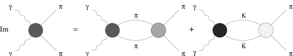
Figure 1: The relation between the two photon amplitudes and those for hadronic reactions given by Eq. (7).

$T$–invariance of the strong interactions means

$${\cal T}_{J}^{I}(K\overline{K}\to\pi\pi)\,\equiv\,{\cal T}_{J}^{I}(\pi\pi\to K\overline{K})\;.$$

The analytic properties of the ${\cal F}^{I}_{J\lambda}(s)$ suggest the functions ${\overline{\alpha}}(s)$ are smooth for $s\geq 4m_{\pi}^{2}$, aside from possible poles that can occur in well-defined situations that we will discuss in more detail below. Notice that the $\overline{\alpha}_{\pi,K}(s)$ give the weight with which ${\cal T}^{I}_{J}(\pi\pi\to\pi\pi)$ and ${\cal T}^{I}_{J}(\pi\pi\to K{\overline{K}})$, respectively, contribute to ${\cal F}^{I}_{J\lambda}(\gamma\gamma\to\pi\pi)$. The $\overline{\alpha}_{\pi}(s)$ and $\overline{\alpha}_{K}(s)$ will be determined by fitting the experimental data on $\gamma\gamma\to\pi\pi$, as we describe in Sect. 4.

In Eq. (7) the hadronic amplitudes are independent of the photon helicity $\lambda$, since the channels involve only spinless pions and kaons. Below 1 GeV, where the $K{\overline{K}}$ channel switches off, Eq. (6) can be expressed even more simply as

$${\cal F}_{J\lambda}^{I}(\gamma\gamma\to\pi\pi)\,=\,\overline{a}_{\pi}^{I,J\lambda}\,{\cal T}_{J}^{I}(\pi\pi\to\pi\pi)$$ (8)

where $\overline{a}$ is a real function for $4m_{\pi}^{2}\leq s\leq 4m_{K}^{2}$. Eq. (7) and Eq. (8) are, of course, consistent, since for $4m_{\pi}^{2}<s<4m_{K}^{2}$ :

$${\cal T}^{I}_{J}(\pi\pi\to K{\overline{K}})\,\propto\,{\cal T}^{I}_{J}(\pi\pi\to\pi\pi)$$ (9)

with a real function of proportionality. The use of the representation Eq. (7), throughout the region we consider, will allow us to track through the important $K{\overline{K}}$ threshold region. We stop at 1.4 GeV, since there multi-pion channels (as well as $\eta\eta$) become increasingly important and the unitarity constraint, Eq. (6), more complicated and impossible to implement without detailed partial wave information on $\pi\pi\to 4\pi$, $6\pi$, etc.

Though unitarity imposes Eq. (7), for each spin and isospin, in practice the $I=2$ amplitudes are simpler, as a result of the final state interactions being weaker and the $K{\overline{K}}$ channel not being accessible. Consequently, the representation, Eq. (7), will only be used for the $I=0$ $S$ and $D$–waves. Let us deal with these in turn:

• $I=0$ $S$–wave: The $\gamma\gamma$ partial wave amplitude ${\cal F}^{0}_{00}$ will be parametrized in terms of the two real coupling functions $\overline{\alpha}_{\pi}^{0,00}$ and $\overline{\alpha}_{K}^{0,00}$ (denoted by $\overline{\alpha}_{\pi}^{0}$, $\overline{\alpha}_{K}^{0}$ as a shorthand) and the hadronic $S$–wave amplitudes ${\cal T}_{S}(\pi\pi\to\pi\pi)$ and ${\cal T}_{S}(\pi\pi\to K{\overline{K}})$. The input for the hadronic amplitudes is based on a modification (and extension) of the $K$–matrix parametrization of AMP [18]. Briefly, the ${\bf T}$–matrix is related to the ${\bf K}$–matrix by

  $${\bf{\cal T}}\,=\,\frac{{\bf K}}{{\bf 1}\,-\,i{\bf\rho K}}$$ (10)

  where ${\bf\rho}$ is the diagonal phase–space matrix. In the case in which two channels are considered, we have

  $${\bf\rho}\,=\,\left(\begin{array}[]{cc}\rho_{1}&0\\ 0&\rho_{2}\end{array}\right)\;,$$ (11)

  where

  $$\rho_{1}\,=\,\sqrt{1\,-\,\frac{4m^{2}_{\pi}}{s}}\;,$$ (12)

  $$\rho_{2}\,=\,\frac{1}{2}\,\sqrt{1\,-\,\frac{4m^{2}_{K^{\pm}}}{s}}\,+\,\frac{1}{2}\,\sqrt{1\,-\,\frac{4m^{2}_{K^{0}}}{s}}\;.$$ (13)

  In this notation, the convention is

  $$1\;\leftrightarrow\;\pi\pi\;,\quad 2\;\leftrightarrow\;K\overline{K}.$$

  Coupled channel unitarity is then fulfilled by the $K$–matrix being real for $s\geq 4m_{\pi}^{2}$. It is then the $K$–matrix elements, $K_{ij}$ that embody the hadronic information. For our $I=0$ $S$–wave, we take the $K_{1}$ solution from ref. [18] above approximately $1.1$ GeV, which is characterized by having only one pole in the ${\bf K}$–matrix in the $1$ GeV energy region. For energies up to about $1$ GeV, we supply the strong interaction amplitudes ${\cal T}_{S}(\pi\pi\to\pi\pi)$ and ${\cal T}_{S}(\pi\pi\to K\overline{K})$ as given by the “Solution 2” obtained in a further refinement of the [18] fit, reported in ref. [19]. It includes a larger set of experimental data, particularly in the $K\overline{K}$ threshold region, which favour a parametrization of the $f_{0}(980)$ that allows for two poles in the $T$–matrix on different sheets corresponding to this state. These solutions are smoothly joined from one energy region to the other. The moduli of the amplitudes ${\cal T}_{S}(\pi\pi\to\pi\pi)$ and ${\cal T}_{S}(\pi\pi\to K\overline{K})$ determined in this way are shown in Fig. 1. In fact, we have two $K$–matrix parametrizations of these, called ReVAMP1 and 2  [19], in which the $K$–matrix elements, in addition to having a single pole, have either 2nd or 3rd order polynomials, respectively.

   

  Figure 2: Strong interaction inputs for the $I=0$ $S$–wave: here we show the moduli of the amplitudes ${\rm T}$, which are obtained from the amplitudes ${\cal T}$ by removing the Adler zero factor, ${\rm T}(s)={\cal T}(s)/(s-s_{0})$.

  The relation of these hadronic amplitudes to that for $\gamma\gamma\to\pi\pi$ is through the coupling functions $\overline{\alpha}_{\pi,K}$. Since these functions have only left hand cuts, they must be real for $s\geq 4m_{\pi}^{2}$, but should be smooth along the right hand cut, once obvious dynamical structures are taken into account. Such obvious structures are that the coupling functions have poles wherever any element, or other sub-determinant, of the $T$–matrix has a real zero. For instance, ${\cal T}_{S}(\pi\pi\to\pi\pi)$ and ${\cal T}_{S}(\pi\pi\to K{\overline{K}})$ have Adler zeros below threshold (at $s=s_{0}$), which are not present in the $\gamma\gamma$ amplitude. (That is why they have been divided out in the amplitudes plotted in Fig. 2) Similarly, ${\rm{det}}{\bf{\cal T}}(s)$ can (and in fact does) vanish at a real value of $s=s_{1}$, where $s_{1}\leq 4m_{K}^{2}$ because of Eq. (9). Unless the $\overline{\alpha}$’s have poles at this point, with related residues, this constraint on the hadronic amplitudes unnecessarily transmits to the $\gamma\gamma$ amplitudes. To avoid these unnatural constraints, the functions are parametrized as follows:

  $$\overline{\alpha}^{0}_{\pi}(s) = \frac{\alpha^{S}_{\pi}(s)}{s-s_{0}}\,+\,\frac{\nu}{s-s_{1}}\,{\cal T}_{S}(\pi\pi\to K{\overline{K}};s=s_{1})\;,$$

  $$\overline{\alpha}^{0}_{K}(s) = \frac{\alpha^{S}_{K}(s)}{s-s_{0}}\,-\,\frac{\nu}{s-s_{1}}\,{\cal T}_{S}(\pi\pi\to\pi\pi;s=s_{1})\;.$$ (14)

  The fit then determines $\alpha_{\pi}^{S}$ and $\alpha_{K}^{S}$ as polynomials in $s$ and the constant parameter $\nu$. It is important to stress that the poles in Eq. (14) do not appear in the $\gamma\gamma$ amplitudes, of course. This representation, Eq. (7), for the $I=0$ $S$–wave has the flexibility needed to determine the details of the mechanism by which the scalar resonances, $f_{0}$’s, couple to two photons.

• $I=0$ $D$–waves with $\lambda=0,2$: here a simplification arises from the fact that the $\pi\pi\to\pi\pi$ and $\pi\pi\to K{\overline{K}}$ amplitudes are proportional to each other, both being dominated by the $f_{2}(1270)$ resonance. Then the hadronic amplitude ${\cal T}_{D}(\pi\pi\to\pi\pi)$ is given by

  $${\cal T}_{D}(\pi\pi\to\pi\pi)\,=\,\frac{BR}{\beta(m_{f}^{2})}\,\frac{m_{f}\ \Gamma(s)}{m_{f}^{2}-s-im_{f}\Gamma(s)}\;$$ (15)

  where $BR$ is the branching ratio of $f_{2}\to\pi\pi$. Importantly, the width is energy dependent and given by

  $$\Gamma(s)\,=\,\frac{\beta(s)}{\beta(m_{f}^{2})}\,\Gamma_{\rm tot}\,D_{2}(s)$$ (16)

  with $\beta(s)=\sqrt{1-4m_{\pi}^{2}/s}$. The factor $D_{2}(s)$ incorporates threshold and barrier effects. Here, we take these to be given by duality shaping, with the scale set by the slope of the non-strange Regge trajectories (or equivalently the $\rho$–mass, $m_{\rho}$). Then

  $$D_{2}(s)\,=\,{\left(1+\frac{6m_{\rho}^{2}}{(m_{f}^{2}-4m_{\pi}^{2})}+\frac{6m_{\rho}^{4}}{(m_{f}^{2}-4m_{\pi}^{2})^{2}}\right)}/{\left(1+\frac{6m_{\rho}^{2}}{(s-4m_{\pi}^{2})}+\frac{6m_{\rho}^{4}}{(s-4m_{\pi}^{2})^{2}}\right)}\;.$$

  The $\pi\pi\to K{\overline{K}}$ amplitude is proportional to this and so (just as in Eq. (8)) we can write

  $${\cal F}_{2\lambda}\,=\,\overline{\alpha}^{0,2\lambda}(s)\,{\cal T}_{D}(\pi\pi\to\pi\pi)\;,$$ (17)

  even above $K{\overline{K}}$ threshold, where the $\overline{\alpha}^{0,2\lambda}(s)$ are again smooth real functions of energy to be determined by the fit to experimental data. To ensure the appropriate threshold behaviour for the $\gamma\gamma\to\pi\pi$ amplitude, these $D$–wave coupling functions are parametrized by modifying the threshold factor, so

  $$\overline{\alpha}^{0,2\lambda}(s)\,=\,\frac{\alpha^{D\lambda}}{\sqrt{D_{2}(s)}}\;.$$ (18)

  $m_{f}$ and $\Gamma_{\rm tot}$ are taken from the PDG Tables [4] and $D_{2}(s)$ as in Eq. (17).

So far the formalism we have described would apply to any reaction, by which a non-strongly interacting initial state leads to $\pi\pi$. We now turn to the particular features of the two photon reaction.

For $\gamma\gamma\to\pi\pi$, Low’s low energy theorem [10] imposes an important constraint, in which the hadron charge fixes the size of the cross-section. This is embodied in the one pion exchange Born amplitude. Though the theorem applies at the threshold for the Compton process $\gamma\pi\to\gamma\pi$, the Born term controls the $\gamma\gamma\to\pi\pi$ amplitude in the whole low energy region [11], as discussed extensively in [3]. It is this dominance of the Born term that means, unusually for a strong interaction final state, that the $I=2$ channel is just as important as that with $I=0$. It is the almost exact cancellation between those amplitudes with $I=0,2$ that makes the $\gamma\gamma\to\pi^{0}\pi^{0}$ cross-section small at low energies.

While the Born amplitude controls the low energy process, it is of course modified by final state interactions. As already mentioned these affect the $I=0$ and $I=2$ $\pi\pi$ channels quite differently. For the $I=2$ final state, these interactions are weak and the Born amplitude is little changed, remaining predominantly real in all partial waves. In contrast, the $I=0$ final state interactions in $S$ and $D$ waves are strong (leading to resonance formation for instance), consequently even close to $\pi\pi$ threshold the Born amplitude is modified. It is unitarity that allows these modifications to be reliably calculated up to 600 or 700 MeV [11, 3]. Consequently, the Born amplitude, with such modifications from final state interactions, provides a precise description of the partial wave amplitudes on to which we must connect our amplitude analysis.

• All waves with spin $J\geq 4$: For these, final state interactions are negligible and so the $\gamma\gamma\to\pi\pi$ amplitudes are set equal to the Born amplitude in the whole energy region up to 1.4 GeV. Thus

  $${\cal F}_{J\lambda}\,(\gamma\gamma\to\pi^{+}\pi^{-})\,=\,B_{J\lambda}\,(\gamma\gamma\to\pi^{+}\pi^{-})\;,$$ (19)

  and

  $${\cal F}_{J\lambda}\,(\gamma\gamma\to\pi^{0}\pi^{0})\,=\,B_{J\lambda}\,(\gamma\gamma\to\pi^{0}\pi^{0})\,=\,0\;.$$ (20)

• $I=2$ $S$ and $D$ waves: Here the $\gamma\gamma\to\pi\pi$ amplitudes have modifications from final state interactions that can be calculated up to 1.4 GeV. This we do by expressing the amplitude essentially as a modulus times a phase factor as

  $${\cal F}^{I=2}_{J\lambda}(s)\,=\,\sqrt{\frac{1}{3}}\,P^{B}_{J\lambda}(s)\,\Omega^{I=2}_{J\lambda}(s)\;,$$ (21)

  where $\Omega^{I=2}_{J\lambda}(s)$ is the appropriate Omnès function [20]:

  $$\Omega_{J\lambda}^{I}(s)\,=\,\exp\left[\frac{s}{\pi}\int_{4m^{2}_{\pi}}^{\infty}ds^{\prime}\,\frac{\phi_{J\lambda}^{I=2}(s^{\prime})}{s^{\prime}(s^{\prime}-s)}\right]\;,$$ (22)

  with $\phi_{J\lambda}^{I=2}$ the phase of the corresponding $\gamma\gamma$ amplitudes ${\cal F}^{I=2}_{J\lambda}$. Applying elastic unitarity relates this phase to the $I=2$ spin $J$ $\pi\pi$ phase shift. Then, using the data of Ref. [21], the $\Omega$’s are readily computed. The function $P(s)$ in Eq. (21) is then real for $s\geq 4m_{\pi}^{2}$ and can be calculated as follows. Dropping the $I,\lambda$ indices to keep the notation simple, consider the analytic function $f_{J}(s)$ defined by

  $$f_{J}(s)\,=\,B_{J}(s)\,(\Omega_{J}^{-1}(s)\,-\,1)\;,$$ (23)

  where $B_{J}(s)$ is the spin $J$ Born amplitude. We now write a once subtracted dispersion relation for $f_{J}(s)/(s-4m_{\pi}^{2})^{J/2}$

  $$f_{J}(s)\,=\,f_{J}(0) + \frac{s(s-4m_{\pi}^{2})^{J/2}}{\pi}\,\int^{\infty}_{4m_{\pi}^{2}}ds^{\prime}\frac{B_{J}(s^{\prime})\,{\rm Im}\Omega_{J}^{-1}(s^{\prime})}{s^{\prime}(s^{\prime}-s)(s^{\prime}-4m_{\pi}^{2})^{J/2}}$$ (24)

  $$+ \frac{s(s-4m_{\pi}^{2})^{J/2}}{\pi}\,\int_{-\infty}^{0}\frac{{\rm Im}[B_{J}(s^{\prime})(\Omega_{J}^{-1}(s^{\prime})-1)]}{s^{\prime}(s^{\prime}-s)(s^{\prime}-4m_{\pi}^{2})^{J/2}}\;,$$

  where we have taken into account that $B_{J}(s)$ has only a cut on the left-hand side, so that

  $$\begin{array}[]{lll}{\rm Im}\ f_{J}(s)\,=\,B_{J}(s)\,{\rm Im}\Omega_{J}^{-1}(s)&\;\;{\rm for}&s\geq 4m_{\pi}^{2}\;,\\ &&\\ {\rm Im}\ f_{J}(s)\,=\,{\rm Im}\,[B_{J}(s)\,(\Omega_{J}^{-1}(s)-1)]&\;\;{\rm for}&s<0\;.\end{array}$$

  If we use the fact that $f_{J}(0)=0$ since $\Omega(0)=1$, and subtract the function $P(s)$ from Eq. (24), we find

  $$P_{J}(s)\,=\,B_{J}(s)\,+\,\frac{s(s-4m_{\pi}^{2})^{J/2}}{\pi}\,\int^{\infty}_{4m_{\pi}^{2}}ds^{\prime}\frac{B_{J}(s^{\prime})\,{\rm Im}\Omega_{J}^{-1}(s^{\prime})}{s^{\prime}(s^{\prime}-s)(s^{\prime}-4m_{\pi}^{2})^{J/2}}$$ (25)

  which involves the integration of the imaginary part of the function $\Omega_{J}^{-1}(s)$ over the right–hand cut only. This allows us to use hadronic information for $s\geq 4m_{\pi}^{2}$ to constrain the input into our description of the limited $\gamma\gamma\to\pi\pi$ experimental results.

  The factor $\sqrt{1/3}$ in Eq. (21) is the appropriate Clebsch–Gordan coefficient, as obtained by decomposing the amplitudes with definite isospin in terms of the amplitudes with definite charge quantum numbers. As a consequence of the fact that the $\pi^{0}\pi^{0}$ Born amplitude is zero, we have:

  $$B(\gamma\gamma\to\pi^{0}\pi^{0})\,=\,\sqrt{\frac{2}{3}}\,B^{I=2}-\sqrt{\frac{1}{3}}\,B^{I=0}=0\;,$$ (26)

  from which

  $$B^{I=0}\,=\,\sqrt{2}\,B^{I=2}\;.$$ (27)

  Applying this to the Born amplitude

  $${\cal B}\,\equiv\,B(\gamma\gamma\to\pi^{+}\pi^{-})\,=\,\sqrt{\frac{2}{3}}\,B^{I=0}+\sqrt{\frac{1}{3}}\,B^{I=2}$$ (28)

  we have

  $$B^{I=2}\,=\,\sqrt{\frac{1}{3}}\,{\cal B}\;\;,\;\;\;B^{I=0}\,=\,\sqrt{\frac{2}{3}}\,{\cal B}\;.$$ (29)

• $I=0$ $S$ and $D$ waves: For these, an identical procedure can be used to calculate the modifications from final state interactions reliably up to 0.6 GeV, starting from

  $${\cal F}^{I=0}_{J\lambda}(s)\,=\,\sqrt{\frac{2}{3}}\,P^{B}_{J\lambda}(s)\,\Omega^{I=0}_{J\lambda}(s)\;,$$ (30)

  and using information about the $I=0$ $S$ and $D$ waves $\pi\pi$ phase-shift [22, 3] to compute the $\Omega$’s. Below 600 MeV, the effect of the unknown $\gamma\gamma\to\pi\pi$ isoscalar phases in the inelastic regime above 1 GeV is small — see Ref. [23]. The effect of the modification from final state interactions is shown for example in Fig. 3. At higher energies, non-pion exchange contributions become increasingly important as discussed in [3] and so these partial waves can no longer be reliably calculated from first principles. Instead, we leave the data to determine the amplitudes using the representation given by Eq. (7).

Let us summarize the input and the constraints, in the region under study. Everywhere, all the $I=2$ partial waves and the $I=0$ waves with $J\geq 4$ are given by the modified Born amplitudes. Final state interactions only appreciably affect the $I=0$ $S$ and $D$ waves. The $I=0$ waves with $J=0,2$ can be reliably predicted by the modified Born amplitudes below 600 MeV. However, everywhere they can be represented by Eq. (7) which follows merely from coupled channel unitarity.

With the hadronic amplitudes $\cal{T}_{S}$ and $\cal{T}_{D}$ known, the four coupling functions $\alpha^{S}_{\pi}$, $\alpha^{S}_{K}$, $\alpha^{D\lambda}$ are what the data and the above constraints determine. These four $\alpha$’s are polynomials in energy, which we allow to be at most cubic: this gives a reasonable degree of flexibility, but without an overdue number of unphysical structures that could affect the reliability of the fit. They are written as a Legendre expansion in terms of the variable $x$, defined as

$$x\,=\,\frac{2E-E_{1}-E_{2}}{E_{2}-E_{1}}\quad,$$ (31)

so that the energy interval {$E_{1}=0.28,E_{2}=1.44$}, which gives the boundaries of the energy range we are fitting, maps onto the interval $-1\leq x\leq 1$. Symbolically, we write each $\alpha$ as

$$\alpha_{i}\,=\,\sum_{n=0}^{3}\alpha^{(n)}_{L}P_{n}(x)\;.$$ (32)

Before we consider the data we are going to analyse to determine their partial wave content, let us stress that there is an important region below 600 MeV, where the $\gamma\gamma\to\pi\pi$ amplitudes are predicted and must also agree with the unitary representation of Eq. (7). These predictions provide a reliable starting point for such a general representation. We next describe how we build in this constraint.

3 Analysis procedure

3.1 Low energy inputs

To implement the constraint from Low’s theorem [10], that as we go down in energy the amplitudes are given by their Born terms [11], we adopt the following strategy.

 

Figure 3: The amplitudes ${\cal F}^{I=0}_{J\lambda}$ in the low energy region. The shaded areas represent the bands we give as a constraining input, by building a “horn”around the central curve generated by the final state modified Born amplitudes. The solid lines are the output of our fit. For this plot we have used, as an illustration, the outcomes corresponding to what is later called the peak solution; but the difference between the two solutions in the low energy range is hardly noticable.

We take the $[{\cal F}^{I=0}_{J\lambda}]_{\rm low\;energy}$ below 600 MeV, as calculated in Sect. 2. Our amplitudes, fitted to experiment, must agree with these within some tolerance. To fix this, we construct a “horn” around the curves given by ${\cal F}^{I=0}_{J\lambda}(s)$, by assigning error bars, which are zero at threshold and become progressively larger as the energy increases. This reflects the fact that neglecting other exchanges then the pion becomes a poorer approximation as the energy increases. To do this we introduce a contribution to the total $\chi^{2}$ from fitting

$$\chi^{2}_{\rm low\;energy}\,=\,\left(\frac{[{\cal F}^{I=0}_{J\lambda}]_{\rm trial\;form}-[{\cal F}^{I=0}_{J\lambda}]_{\rm low\;energy}}{\Delta{\cal F}}\right)^{2}\;,$$ (33)

where $\Delta{\cal F}$ is obviously given by the errors on $[{\cal F}^{I=0}_{J\lambda}]_{\rm low\;energy}$ we have introduced. These ensure an extremely tight constraint close to $\pi\pi$ threshold, while allowing larger flexibility when the two photon energy approaches $500-600$ MeV. Fig. 3 illustrates how the amplitudes ${\cal F}^{I=0}_{J\lambda}$ determined by our fit fulfil the low energy constraints given by the Born amplitudes modified by final state interactions of Eq. (32). The shaded regions are the “horns” inside which the low energy amplitudes ${\cal F}^{I=0}_{J\lambda}$ are required to fall.

3.2 Data analysis

As mentioned in the introduction, the data-sets on two photon scattering into charged pion final states at low energies come from Mark II [8] and CELLO [12], whereas two different runs of the Crystal Ball experiment, the last with much higher statistics, provide the only available normalized experimental information on $\gamma\gamma\to\pi^{0}\pi^{0}$ for such low energies. Table 1 shows the number of data in each experiment, below 1.4 GeV.

Experiment	Process	Int. X-sect.	$|\cos\theta|_{max}$	Ang. distrib.	$|\cos\theta|_{max}$
Mark II	$\gamma\gamma\to\pi^{+}\pi^{-}$	87	0.6	69	0.6
Cr. Ball	$\gamma\gamma\to\pi^{0}\pi^{0}$	26	0.8 (CB88) 0.7 (CB92)	80	0.8
CELLO	$\gamma\gamma\to\pi^{+}\pi^{-}$	30	0.6	127 (Harjes) 249 (Behrend)	0.55 - 0.8

Table 1: Number of data in each experiment below 1.4 GeV. Mark II results are from Boyer et al. [8], Crystal Ball from Marsiske et al. (CB88) [7] and Bienlein et al. (CB92) [13], and CELLO from Harjes [24] and Behrend et al. [12].

Though the angular distributions contain information about the integrated cross-section, because of different bin centres and sizes, these are not always the same. For instance, Mark II gives the angular distributions for $|\cos\theta|\leq 0.6$ in energy bins of 100 MeV, but present the integrated cross-section in 10 MeV steps above 750 MeV.

From the CELLO experiment, we have angular distributions in $\Delta\cos\theta$ bins of 0.05 from Behrend et al. [12] and $\Delta\cos\theta$ bins of 0.1 from the thesis of Harjes [24], both in energy bins of 50 MeV width. Though these come from the same data sample we believe, we have fitted them as separate data-sets but weighted appropriately (see later), since the different binning produces quite a difference in the scatter of the data-points, see Fig. 4.

 

Figure 4: Comparison between the angular distribution of CELLO data-points on $\gamma\gamma\to\pi^{+}\pi^{-}$ from Behrend [12] (squares) and Harjes [24] (diamonds) for some illustrative energy bins ($E$ is in GeV).

Where statistical and systematic errors are quoted (see tables in [2]), these have been added in quadrature. Each experiment has an absolute normalization for the cross-sections. However, these inevitably provide additional systematic uncertainties. Such uncertainties have been included in the results produced by the special low energy triggering of Mark II. However, above 700 MeV a systematic shift in normalization is apparent between the Mark II and CELLO integrated cross sections, though both of them are for $|\cos\theta|\leq 0.6$, see Fig. 5. It is clear that we must allow for some systematic shift in normalization, if we are to describe both data-sets in a sensible way. Mark II quote a systematic normalization uncertainty of 7%. With this in mind, we allow for up to a $5\%$ relative shift in normalization between Mark II and CELLO experiments.

 

Figure 5: Comparison between Mark II [8] (diamonds) and CELLO [12] (squares) integrated cross-sections for $\gamma\gamma\to\pi^{+}\pi^{-}$ in their common energy range.

 

Figure 6: Comparison between CB88 [7] (diamonds) and CB92 [13] (squares) integrated cross-sections for $\gamma\gamma\to\pi^{0}\pi^{0}$.

For the $\pi^{0}\pi^{0}$ channel, Crystal Ball had two distinct runs. The first covering the energy region from $\pi\pi$ threshold, called CB88 [7]. The second had 1.5 times as much data, but only above 800 MeV. Bienlein et al. [13] combined this with the CB88 set to produce their complete CB92 dataset above 800 MeV. Nevertheless, there was always a clear systematic difference in the earlier and later runs through the $f_{2}$–region. The CB88 set had a higher, narrower peak than the combined CB92 set (see Fig. 6). Since the CB88 set (above 800 MeV) is subsumed in CB92, we cannot really separate them. Consequently, we allow for a systematic shift of $3\%$ between CB88 below 800 MeV and CB92 above.

While both charged and neutral pion experiments would be consistent (and the fits even better) with larger normalization shifts, we have erred on the side of caution in allowing this freedom. To repeat : we assume that the results from CELLO, CB88 below 800 MeV and Mark II below 400 MeV are absolute, and allow small shifts of other data-sets with respect to these.

3.3 Weighting, relative normalizations and fitting

From Table 1, we see that the number of data-points is far greater for the reaction $\gamma\gamma\to\pi^{+}\pi^{-}$ than for $\gamma\gamma\to\pi^{0}\pi^{0}$. Since an accurate separation of the $I=0$ component requires both are accurately described, we give different weight factors to each dataset. We choose these so that the Mark II and the CELLO data have roughly the same number of weighted data, while the weight assigned to the Crystal Ball data approximately equals the weighted sum of the Mark II and CELLO data. Nevertheless, good agreement is not easy to achieve.

The analysis program (GAMP [9]) works by integrating the amplitudes over the appropriate bin in energy and angle for each data-point. It does not just use the central values. This is to allow for any strong local variation of the amplitudes, particularly near $K{\overline{K}}$ threshold. In the next Section, where we display the solutions we find, this should be borne in mind. Where the energy bins are sizable (as with Crystal Ball), histograms are plotted (see Figs. 8 and 11). Where the energy bins are fine (as with Mark II data in 10 MeV steps), the fits are shown more appropriately as continuous lines joining the bin centres, as in Figs. 7, 9, 10, 12. However throughout, the fits are histograms.

4 Results

Our fits deliver two classes of distinct solutions. As is seen from Figs. 7-18, the two classes have very similar quality as far as fitting the data is concerned, yet they have quite distinct characteristics. The first has a peak in the cross–section located in the $1$ GeV energy region and from now on will be referred to as the peak solution. The second has a dip in the same energy region and will be called the dip solution. The plots with the fits to the Mark II $\pi^{+}\pi^{-}$ integrated cross-section look more structured than those of CELLO in the 1 GeV region (cf. Figs 7 and 9, or 10 and 12). This is because our fitting routine integrates over bins, which for Mark II are only 10 MeV wide in this region compared with 25 MeV from CELLO. Detailed dynamical features are picked up more strongly in the finer binned data. Recall the fits are not continuous curves but histograms, as shown in Figs. 8, 11 for the $\pi^{0}\pi^{0}$ data of Crystal Ball.

Looking at the plots of just the Mark II results, Figs 7, 10, on the integrated cross-section for $\gamma\gamma\to\pi^{+}\pi^{-}$ in the 1 GeV region, one might be tempted to conclude that the peak solution is disfavoured. However, one cannot conclude that from the CELLO results, Figs. 9, 12, on the same channel and Crystal Ball, Figs. 8, 11, on the $\pi^{0}\pi^{0}$ final state, nor indeed from looking at the fits over the whole energy region for Mark II. Thus, individual features are a poor guide, even though one’s eye naturally picks those out. Indeed, the overall quality of the fits in each sector for the two distinct solutions are quite comparable as can be seen from Tables 2 and 3. There we report the contributions to the total $\chi^{2}$ from each experimental set, for the integrated cross-section and the angular distribution separately for the best of these solutions. This total is expressed as the $\chi^{2}$ per degree of freedom. The peak solution has a slightly lower overall $\chi^{2}$. However, the CELLO data turn out to be easiest to fit (and so we have reduced their weight by 1/2 to achieve greater sensitivity to the rest). In contrast, the two solutions have appreciably greater $\chi^{2}$ for the Mark II and Crystal Ball results by $\sim 0.5$ per degree of freedom.

PEAK SOLUTION $\chi^{2}_{{\rm tot}}=1.40$
Experiment	Process	data-points	$\chi^{2}_{{\rm average}}$	Int. X-sect.	Ang. distrib.
Mark II	$\gamma\gamma\to\pi^{+}\pi^{-}$	156	1.54	$\chi^{2}$ = 1.82	$\chi^{2}$ = 1.19
Cr. Ball	$\gamma\gamma\to\pi^{0}\pi^{0}$	106	1.44	$\chi^{2}$ = 1.42	$\chi^{2}$ = 1.44
CELLO	$\gamma\gamma\to\pi^{+}\pi^{-}$	406	1.33	$\chi^{2}$ = 0.65	$\chi^{2}$ =1.13 from Harjes $\chi^{2}$ =1.52 from Behrend

Table 2: Summary of contributions from each experiment to the total $\chi^{2}$ for the peak solution. Here $\chi^{2}_{\rm tot}$ is calculated by dividing the sum of the $\chi^{2}$’s for all data-sets by the total number of data-points we are fitting, namely 668. $\chi^{2}_{\rm average}$ is computed by dividing the sum of the $\chi^{2}$’s for each data-set by the total number of data-points in that experiment.

DIP SOLUTION $\chi^{2}_{{\rm tot}}=1.48$
Experiment	Process	data-points	$\chi^{2}_{{\rm average}}$	Int. X-sect.	Ang. distrib.
Mark II	$\gamma\gamma\to\pi^{+}\pi^{-}$	156	1.75	$\chi^{2}$ = 1.99	$\chi^{2}$ = 1.46
Cr. Ball	$\gamma\gamma\to\pi^{0}\pi^{0}$	106	1.62	$\chi^{2}$ = 1.97	$\chi^{2}$ = 1.51
CELLO	$\gamma\gamma\to\pi^{+}\pi^{-}$	406	1.33	$\chi^{2}$ = 0.88	$\chi^{2}$ =1.09 from Harjes $\chi^{2}$ =1.51 from Behrend

Table 3: Summary of contributions from each experiment to the total $\chi^{2}$ for the dip solution, as described for Table 2.

Figure 7: Cross-section as a function of the $\pi\pi$ invariant mass integrated over $\mid\cos\ \theta\mid\;\leq\;0.6$, and angular distributions as a function of $\cos\ \theta$, for the $\gamma\gamma\rightarrow\pi^{+}\pi^{-}$ process, from the MARK II experiment [8] (peak solution).

Figure 8: Cross-section as a function of the $\pi\pi$ invariant mass integrated over $\mid\cos\ \theta\mid\;\leq\;0.8$ for $E\,\leq\,0.8\,$GeV and $\mid\cos\ \theta\mid\;\leq\;0.7$ for higher energies, and angular distributions as a function of $\cos\ \theta$, for the $\gamma\gamma\rightarrow\pi^{0}\pi^{0}$ process, from the CRYSTAL BALL experiment [7, 13] (peak solution).

Figure 9: Cross-section as a function of the $\pi\pi$ invariant mass integrated over $\mid\cos\ \theta\mid\;\leq\;0.6$, and angular distributions as a function of $\cos\ \theta$, for the $\gamma\gamma\rightarrow\pi^{+}\pi^{-}$ process, from the CELLO experiment (peak solution). The angular distributions are from the binning of Harjes [24] — see Fig. 13 for the Behrend et al. binning.

Figure 10: Cross-section as a function of the $\pi\pi$ invariant mass integrated over $\mid\cos\ \theta\mid\;\leq\;0.6$, and angular distributions as a function of $\cos\ \theta$, for the $\gamma\gamma\rightarrow\pi^{+}\pi^{-}$ process, from the MARK II experiment [8] (dip solution).

Figure 11: Cross-section as a function of the $\pi\pi$ invariant mass integrated over $\mid\cos\ \theta\mid\;\leq\;0.8$ for $E\,\leq\,0.8\,$GeV and $\mid\cos\ \theta\mid\;\leq\;0.7$ for higher energies, and angular distributions as a function of $\cos\ \theta$, for the $\gamma\gamma\rightarrow\pi^{0}\pi^{0}$ process, from the CRYSTAL BALL experiment [7, 13] (dip solution).

Figure 12: Cross-section as a function of the $\pi\pi$ invariant mass integrated over $\mid\cos\ \theta\mid\;\leq\;0.6$, and angular distributions as a function of $\cos\ \theta$, for the $\gamma\gamma\rightarrow\pi^{+}\pi^{-}$ process, from the CELLO experiment (dip solution). The angular distributions are from the binning of Harjes [24] — see Fig. 14 for the Behrend et al. binning.

Figure 13: The angular distributions as a function of $\cos\ \theta$, for the $\gamma\gamma\rightarrow\pi^{+}\pi^{-}$ process, in different $\pi\pi$ mass bins from the Behrend et al. analysis [12] of CELLO experiment for the peak solution, to be compared with Figs. 9, 12, where the bins in $\cos\theta$ are larger.

Figure 14: As for Fig. 13, but showing the dip solution.

To explore the neighbourhood of these best fits, it is convenient to characterise these classes of solutions by the relative amount of $I=0$ $S$, $D_{0}$ and $D_{2}$ contribution to the cross-section $\sigma=\sigma_{S}+\sigma_{D_{0}}+\sigma_{D_{2}}$ at the $f_{2}(1270)$ peak. Each solution corresponds to a point in the equilateral triangle of height 1 with sides $\sigma_{S}/\sigma=0$, $\sigma_{D_{0}}/\sigma=0$ and $\sigma_{D_{2}}/\sigma=0$ (see Figs. 15, 16). For the two classes of solutions, peak and dip, we display the overall $\chi^{2}$ per degree of freedom found for each fit in these equilateral triangles.

These diagrams, Figs. 15, 16, clearly show that the fit singles out a well defined region in the parameter space for each class. If we tried to drive them outside this area, their $\chi^{2}$ values would increase very rapidly. Each rectangular flag in Figs. 15, 16 indicates one solution is found at that particular point, and the number which labels it is the corresponding $\chi^{2}$. The round labels indicate the position of solutions $A$ (the typical “good” solution) and $B$ (technically the “best” solution) found by Morgan and Pennington in their previous $\gamma\gamma\to\pi\pi$ data analysis [9]. Notice how, while their favoured solution $A$, falls inside the region determined by both our classes of solutions, their best solution $B$, having very large $S$ and $D_{0}$ wave contributions at the $f_{2}(1270)$ peak, lies considerably far away from it.

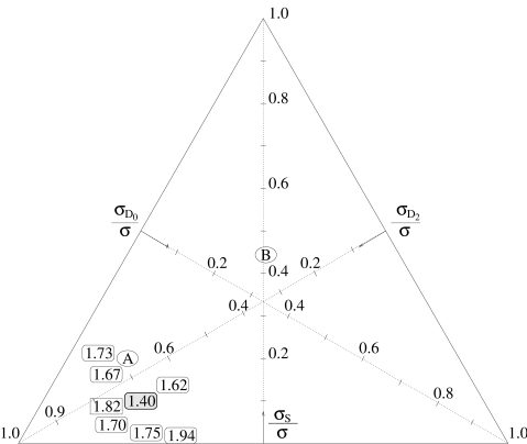
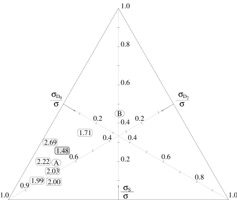
Figure 15: Mapping of an assortment of solutions with different proportions of $\sigma_{S}$, $\sigma_{D_{0}}$ and $\sigma_{D_{2}}$ at 1270 MeV labelled by the $\chi^{2}$ per dof for the peak class.

Figure 16: Mapping of an assortment of solutions with different proportions of $\sigma_{S}$, $\sigma_{D_{0}}$ and $\sigma_{D_{2}}$ at 1270 MeV labelled by the $\chi^{2}$ per dof for the dip class.

If we now compare the diagrams in Figs. 15 and 16, we see that our peak class of solutions singles out a region in the parameter space where the $\sigma_{S}/\sigma$ components are remarkably small, approximately bounded by

$$0.00 <\;\sigma_{S}/\sigma\;< 0.25\;,$$

$$0.06 <\;\sigma_{D_{0}}/\sigma\;< 0.35\;.$$ (34)

Alternatively, the dip class of solutions determine a region the boundaries of which are given by higher values of $\sigma_{S}/\sigma$ and lower values of $\sigma_{D_{0}}/\sigma$:

$$0.11 <\;\sigma_{S}/\sigma\;< 0.35\;,$$

$$0.03 <\;\sigma_{D_{0}}/\sigma\;< 0.16\;.$$ (35)

Furthermore, in Tables 4 and 5 we report the $\chi^{2}$’s of two representative solutions from the peak and dip classes, to be compared with those corresponding to our two favoured solutions, respectively, shown in Tables 2 and 3. They have been picked out from the solutions lying in the regions of the parameter space shown in Figs. 15 and 16 in order to show the difference in the $\chi^{2}$’s corresponding to each data set for an ordinary solution in either the peak or the dip class compared to our best solution (indicated by the shaded flag). It is immediately evident how the $\chi^{2}$’s corresponding to the CELLO experimental data, not only the overall averaged one but also the individual $\chi^{2}$ for the integrated cross section and the angular distribution, hardly change at all. On the contrary, big variations occur for the other data-sets, the $\chi^{2}$ of which in some cases increase by a factor of $2$. Indeed, it is all the data-sets together that determine the features of the solutions, but we once again want to stress the point that while a remarkably good agreement with the CELLO data is easily achieved most of the time, the Crystal Ball and Mark II data are always hard to satisfy simultaneously. In fact, as seen from Figs. 9 and 12, the CELLO data have finer energy and angular bins. Consequently, it is these data that most powerfully constrain our solutions. Thus the solutions in Tables 2–5 all have very similar $\chi^{2}$ for this sector, and it is in the contributions to $\chi^{2}$ from the Mark II and Crystal Ball data-sets that they differ. A final comment ought to be made on the contribution to the total $\chi^{2}$ from the low energy region constraints. As we have seen in Fig. 3, the agreement of the fit solutions to the low energy amplitudes ${\cal F}^{I=0}_{J\lambda}$, calculated by a dispersion relation over the right–hand cut, is pretty good. The ratio of the low energy $\chi^{2}$, see Eq. (33), to the total overall $\chi^{2}$ is the following

$$\,\;{\chi^{2}_{\rm low\;energy}}/{\chi^{2}_{\rm tot}}\,=\,0.22\qquad\;\;{\rm for\;the\;{\it peak}\;solution}\;,$$ (36)

$${\chi^{2}_{\rm low\;energy}}/{\chi^{2}_{\rm tot}}\,=\,0.17\qquad\;\;{\rm for\;the\;{\it dip}\;solution}\;.$$ (37)

Illustrative solution no. 1 $\chi^{2}_{tot}=1.82$
Experiment	$\chi^{2}_{{\rm average}}$	Int. X-sect.	Ang. distr.
Mark II	2.82	3.21	2.32
Cr. Ball	2.30	3.09	2.03
CELLO	1.30	0.64	1.35

Table 4: Summary of contributions from each experiment to the total $\chi^{2}$ for an illustrative solution in the peak class (see Fig. 15) to be compared with the best solution in that class. See text for comments.

Illustrative solution no. 2 $\chi^{2}_{tot}=2.00$
Experiment	$\chi^{2}_{{\rm average}}$	Int. X-sect.	Ang. distr.
Mark II	2.87	2.87	2.87
Cr. Ball	2.90	3.71	2.64
CELLO	1.42	0.63	1.49

Table 5: Summary of contributions from each experiment to the total $\chi^{2}$ for an illustrative solution in the dip class (see Fig. 16) to be compared with the best solution in that class. See text for comments.

Figure 17: $I=0$ $\gamma\gamma\to\pi\pi$ cross-section as a function of energy (peak solution). Notice the two pronounced peaks in the $S$ partial wave: the first just above threshold, where it dominates the $\pi^{+}\pi^{-}$ cross–section, and the second corresponding to the $f_{0}(980)$ resonance.

Figure 18: $I=0$ $\gamma\gamma\to\pi\pi$ cross-section as a function of energy (dip solution). Notice the pronounced peak in the $S$ partial wave at threshold, where it dominates the $\pi^{+}\pi^{-}$ cross–section, and the dip corresponding to the $f_{0}(980)$ resonance.

5 Solutions

Figs. 17 and 18 show the dominant partial wave components of the $I=0$ $\gamma\gamma\to\pi\pi$ cross-section for our two favoured solutions. These fall into two classes characterised by having either a peak or a dip in the $S$-wave cross-section in the 1 GeV region, corresponding to two distinct coupling patterns for the $f_{0}(980)$. In the peak solution $\alpha_{K}(s)$ is larger than $\alpha_{\pi}(s)$ in the 1 GeV region so that, in the decomposition given by Eq. (7), the contribution of the hadronic reaction $\pi\pi\to K\overline{K}$ dominates over $\pi\pi\to\pi\pi$ (see Figs. 17 and 2). As a consequence the $f_{0}(980)$ has a larger coupling to $\gamma\gamma\to K\overline{K}$ in the peak solution. However, there is nevertheless a crucial contribution from $\alpha_{\pi}(s)$, and hence of the $\pi\pi\to\pi\pi$ amplitude, which results in the $f_{0}(980)$ peak in this $\gamma\gamma$ amplitude (Fig. 17) being sharper than that seen in $\pi\pi\to K\overline{K}$ (Fig. 2). In the alternative class of solutions, $\alpha_{\pi}^{S}(s)$ dominates over $\alpha_{K}^{S}(s)$ in the 1 GeV region and as is clear from Fig. 18 the $f_{0}(980)$ then manifest itself as a dip as in the $\pi\pi\to\pi\pi$ cross-section (see Fig. 2).

In the energy region above 1 GeV, the cross section is dominated by the $D_{2}$-wave embodied in the $f_{2}(1270)$ resonance. An oversimplified description of individual channels is to ascribe the peak in this region wholly to $f_{2}(1270)$ formation in the $\lambda=2$ state [6]. Such a simplification is often used when trying to extract a $\gamma\gamma$ width for the tensor mesons from a single charge final state with limited angular coverage, when a true amplitude analysis is not possible. Here, as in the earlier analysis by Morgan and Pennington [9], sizable contributions of both $S$ and $D_{0}$ waves in this region are strongly favoured. This is in good agreement with solution A of Ref. [9]: however we do not find such large $S$ and $D_{0}$ contribution as their “technically best” solution, B. We report here $\sigma_{S}/\sigma$ and $\sigma_{D_{0}}/\sigma$ ratios for the $I=0$ cross-sections at 1270 MeV for the best solutions in each class:

$$\left.\begin{array}[]{r}\rule[-5.69046pt]{0.0pt}{25.60747pt}\sigma_{S}/\sigma\,=\,0.13\\ \rule[-14.22636pt]{0.0pt}{34.1433pt}\sigma_{D_{0}}/\sigma\,=\,0.22\end{array}\;\right\}\;{\rm for\;the\;{\it peak}\;solution\;,}$$ (38)

$$\left.\begin{array}[]{r}\rule[-5.69046pt]{0.0pt}{25.60747pt}\sigma_{S}/\sigma\,=\,0.25\\ \rule[-14.22636pt]{0.0pt}{34.1433pt}\sigma_{D_{0}}/\sigma\,=\,0.13\end{array}\;\right\}\;{\rm for\;the\;{\it dip}\;solution\;.}$$ (39)

Notice in Figs. 17, 18 how the influence of the Born term at low energies (modified of course by crucial final state interactions) means that even outside the $f_{0}(980)$ region the $S$-wave cross-section is not simply describable by a Breit-Wigner resonance at 600-1200 MeV, rather its contribution is spread over a wide region.

5.1 $\gamma\gamma$ couplings

We now calculate the $\gamma\gamma$ couplings of the resonant states in the threshold to $1.4$ GeV region that our amplitude analysis determines. We do this by two different methods [9]. The first is based on the analytic continuation of the amplitudes we have found in our fit into the complex $s$-plane to the pole position. This is the only formally correct way of deducing the couplings of any resonance and its outcomes are free from background contamination. The second is a more naive approach based on the Breit-Wigner-like peak height. For the $f_{2}(1270)$, these two methods give nearly identical results, as expected for an uncomplicated and isolated resonance with a relatively nearby second sheet pole. For the $f_{0}(980)$ only the pole method is applicable because of the overlapping of this state with $K\overline{K}$ threshold and the broader $f_{0}(400-1200)$. For this latter broad state, only the “peak height” provides a sensible measure of its $\gamma\gamma$ width, since its pole is too far from the real axis to be reliably located under the approximations needed to perform the analytic continuation, as will be clear from what follows.

To work out the pole residue based definition of the radiative widths, we suppose the strong interaction amplitudes ${\cal T}_{J}(s)$ and the corresponding $\gamma\gamma\to\pi\pi$ amplitudes ${\cal F}(s)$ to be dominated by their pole contribution near the resonance pole, i.e. for $s\sim s_{R}$; then we can write them in the form

$${\cal T}_{J}(\pi\pi\to\pi\pi)(s\sim s_{R}) =\;\;\frac{g^{2}_{\pi}}{s_{R}-s}\;,$$ (40)

$${\cal F}_{J\lambda}(\gamma\gamma\to\pi\pi)(s\sim s_{R}) =\;\;\frac{g_{\gamma}\,g_{\pi}}{s_{R}-s}\;.$$ (41)

It is easy to see that the couplings $g_{\pi}$ and $g_{\gamma}$ can be extracted as the residues of these amplitudes at the resonance pole $s_{R}$. Thanks to the parametrization of the amplitudes ${\cal T}$ in terms of the $K$–matrix elements, as given in Eq. (10), we know their numerator, $N_{\pi}(s)$ and $N_{K}(s)$ respectively, and denominator, $D(s)$, which is the same for the two of them. So we can use the expressions

$${\cal T}_{J}(\pi\pi\to\pi\pi)\;=\;\frac{N_{\pi}(s)}{D(s)}\;,$$ (42)

$${\cal T}_{J}(\pi\pi\to K\overline{K})\;=\;\frac{N_{K}(s)}{D(s)}\;,$$ (43)

and Eq. (7), to write ${\cal F}_{J\lambda}(\gamma\gamma\to\pi\pi)$ as:

$${\cal F}_{J\lambda}(\gamma\gamma\to\pi\pi)\,=\,\frac{\overline{\alpha}^{J\lambda}_{\pi}(s)\,N_{\pi}(s)+\overline{\alpha}^{J\lambda}_{K}(s)\,N_{K}(s)}{D(s)}\;.$$ (44)

Now, in the region nearby $s_{R}$ we can make a Taylor expansion of the function $D(s)$, truncated at the first order

$$D(s\sim s_{R})\simeq D(s_{R})+D^{\prime}(s_{R})(s-s_{R})\,=\,D^{\prime}(s_{R})(s-s_{R})\;,$$ (45)

where by definition $D(s_{R})=0$ at the resonance pole. Finally, by substituting this into Eqs. (42,43) and comparing with Eqs. (40,41), we find

$$g_{\pi}^{2}\,=\,\frac{N_{\pi}(s_{R})}{D^{\prime}(s_{R})}\;,$$ (46)

and

$$g_{\gamma}\,g_{\pi}\,=\,\frac{\overline{\alpha}^{J\lambda}_{\pi}(s_{R})\,N_{\pi}(s_{R})+\overline{\alpha}^{J\lambda}_{K}(s_{R})\,N_{K}(s_{R})}{D^{\prime}(s_{R})}\;,$$ (47)

from which the coupling $g_{\gamma}$ can readily be calculated. The corresponding width is then evaluated using the formula

$$\Gamma^{R}_{\gamma\gamma}({\rm pole})\,=\,\frac{\alpha^{2}\,\beta_{R}\;|g_{\gamma}|^{2}}{4(2J+1)m_{R}}\;,$$ (48)

where $\alpha=1/137$ is the fine structure constant, and $\beta_{R}=(1-4m_{\pi}^{2}/m_{R}^{2})^{1/2}\simeq 1$.

Because of its very large width, the $f_{0}(400-1200)$ coupling to two photons cannot be calculated with this technique, since one cannot reliably continue so far into the complex plane. As an alternative, we give a rough estimate of its width by using an expression based on the standard resonance peak formula

$$\Gamma^{R}_{\gamma\gamma}({\rm peak})\,=\,\frac{\sigma_{\gamma\gamma}({\rm res.\;peak})\,m^{2}_{R}\,\Gamma_{tot}}{8\pi(\hbar c)^{2}(2J+1)BR}\;,$$ (49)

where $BR$ is the hadronic branching ratio for the final state considered.

	$\Gamma(f_{2}(1270))$	$\Gamma(f_{0}(980))$	$\Gamma(f_{0}(400-1200))$
Peak solution	3.04	0.13-0.36	3.0
Dip solution	2.64	0.32	4.7

Table 6: Two photon partial widths in $keV$ for the meson states in our two classes of solutions.

Table 6 shows the results we obtain for the $\gamma\gamma$ widths of the $f_{0}(980)$, $f_{0}(400-1200)$, $f_{2}(1270)$ from either the pole or the peak–height definition, as appropriate, when choosing solution 1 and solution 2, respectively.

The continuation to the second sheet pole for the $f_{0}(980)$ is rather sensitive to the parametrization of the $K$–matrix (and hence of the $T$–matrix, Eq. 10) used. In the ReVAMP analysis [19] described in Sect. 2, the $K$–matrix elements are given by a single pole plus different order polynomials. These each fit the hadronic data equally well. For the dip solution, the $\gamma\gamma$ width for the $f_{0}(980)$ is $0.31$ keV for ReVAMP1, and $0.34$ keV for ReVAMP2, so rather little change. However, for the peak solution for which there is a much stronger interplay between the ${\cal T}_{S}(\pi\pi\to\pi\pi)$ and the ${\cal T}_{S}(\pi\pi\to K\overline{K})$ contributions to Eq. (7), we find a $\gamma\gamma$ width of $0.13$ keV for ReVAMP1 and $0.36$ keV for ReVAMP2. Hence the values in Table 6.

From the variation between different solutions within the classes indicated in Figs. 15 and 16, we estimate that the uncertainty on the $\gamma\gamma$ width of the $f_{2}(1270)$ is $\pm 0.08$ keV within each class of solutions. To this must be added a $5\%$ uncertainty in the absolute normalization. Consequently, it is the difference between solutions (rather than within a given class) that constitutes the major uncertainty, and so we quote

$$\Gamma(f_{2}(1270)\to\gamma\gamma)\,=\,(2.84\,\pm\,0.35)\;{\rm keV}\;.$$ (50)

Whilst this is in good agreement with the PDG’98 estimated value of $(2.8\pm 0.4)$ keV, it is somewhat at variance with the PDG’98 fitted value of $\left(2.44^{+0.32}_{-0.29}\right)$ keV, based on several different analyses [4] of either $\pi^{+}\pi^{-}$ or $\pi^{0}\pi^{0}$ data separately using quite different assumptions. It is important to stress that our value is nearest to a model independent amplitude analysis result one can presently achieve.

The uncertanties on the $\gamma\gamma$ widths of the $f_{0}(980)$ and $f_{0}(400-1200)$ are more problematic. For the $f_{0}(980)$ we quote

$$\Gamma(f_{0}(980)\to\gamma\gamma)\,=\,(0.28\,^{+0.09}_{-0.13})\;{\rm keV}.$$ (51)

However, a decision on whether the dip or peak solution was correct would reduce the uncertainty dramatically.

For the $f_{0}(400-1200)$ the estimate is much cruder and a $50\%$ uncertainty is likely, giving

$$\Gamma(f_{0}(400-1200)\to\gamma\gamma)\,=\,(3.8\,\pm\,1.5)\;{\rm keV}.$$ (52)

Once again discriminating between the classes of solutions would change the central value and reduce the error within these ranges.

What about the composition of these states ? Quite independently, we, of course, know the $f_{2}(1270)$ is the $n\overline{n}$ member of an ideally mixed multiplet. The $\gamma\gamma$ widths of the neutral members are then expected to be in the ratio of the squares of the average squared charges of their constituents, so

$$\Gamma(f_{2}\to\gamma\gamma):\Gamma(a_{2}\to\gamma\gamma):\Gamma(f_{2}^{\prime}\to\gamma\gamma)\,=\,25:9:2\;.$$ (53)

Experiments give ratios very close to this. The prediction for the $\gamma\gamma$ width not only depends on the charges of the constituents to which the photons couple, but to the probability that these constituents annihilate — their overlap. For members of a $q\overline{q}$ multiplet we expect these probabilities should be roughly equal. Experiment for the lowest tensor nonet confirms this. (Any differences can readily be explained by a small departure from ideal mixing — see the Appendix of Ref. [9].)

For the scalars, we need a certain modelling. The simplest would be to assume the lightest scalars are the shadow of the tensor nonet. Then non-relativistically, Chanowitz [25] deduced that the corresponding tensor and scalar two photon widths are related by

$$\Gamma(0^{++}\to\gamma\gamma)\,=\,\left(\frac{15}{4}\right)\times\left(\frac{m_{0}}{m_{2}}\right)^{3}\times\Gamma(2^{++}\to\gamma\gamma)\;,$$ (54)

where the factor of $(m_{0}/m_{2})^{3}$ takes account of the mass splitting. This gives the predictions in Table 7, under the assumption that the $f_{0}$ states are either purely $s{\overline{s}}$ or non-strange $n{\overline{n}}$. Relativistic corrections to Eq. (56) have been computed [26] and found to reduce the ratio $\Gamma(0^{++}\to\gamma\gamma)/\Gamma(2^{++}\to\gamma\gamma)$ by as much as a factor of 2 for light quark systems. An oft-cited alternative structure for the $f_{0}(980)$ is as a $K{\overline{K}}$ molecule [15]. Then though the fourth power of the charge of the constituents is far greater for a $K{\overline{K}}$ molecule than for a simple $s{\overline{s}}$ bound state, the molecule is a much more diffuse system, so that the probability of the kaons annihilating to form photons is strongly suppressed. Thus in the non-relativistic potential model of Weinstein and Isgur [15], computation of the molecular radiative width gives $\Gamma(f_{0}(K{\overline{K}}\to\gamma\gamma))=0.6$ keV [27].

	$n\overline{n}$	$s\overline{s}$	$K\overline{K}$
$\Gamma_{0^{++}}$	4.5	0.4	0.6

Table 7: Two photon partial widths in $keV$ predicted for a conventional $q\overline{q}$ nonet of scalar states and for a $K\overline{K}$ molecule.

Even this may be far too simplistic for these $0^{++}$ states. From the work of Tornqvist [16] (replicated by one of us [28]), we know the dressing of bare $q{\overline{q}}$ states, by the hadrons into which the physically observed mesons decay, is particularly large for scalars. In lattice-speak, their unquenching is a big effect. In a scheme where it’s assumed pseudoscalar meson pairs provide the dominant dressing, the $f_{0}(980)$ has not only an $s{\overline{s}}$ (and smaller $n{\overline{n}}$) component, but a large $K{\overline{K}}$ admixture, too. It is not a case of the physical hadron being either a $q{\overline{q}}$ bound state or a $K{\overline{K}}$ molecule, but it is in fact both! What this non-perturbative treatment predicts for the radiative width of the $f_{0}(980)$ is a calculation under way.

We know there are other scalars beyond the region of our analysis: the $f_{0}(1500)$ and $f_{J}(1710)$ in particular [4]. Some claim there is also an $f_{0}(1370)$. In the past, we have argued that this may just be the higher end of the broad $f_{0}(400-1200)$, cut-off below by $K{\overline{K}}$ and $4\pi$ phase-space. Interestingly, the very recent potential model analysis of Kaminski et al. [29] suggests the $f_{0}(1370)$ may actually be the same as the $f_{0}(1500)$. In any event, the radiative width of all these states is a key pointer to their composition, gluonic or otherwise [17, 30]. At present, only crude estimates are possible, for instance [31] that $\Gamma(f_{0}(1500)\to\gamma\gamma)<0.17$ keV. To achieve something more is the challenge for the future. A major task is to extend the present Amplitude Analysis beyond 1.4 GeV. This requires a study of two photon production of not just two pion final states, but $4\pi$ and $K\overline{K}$ too. Only by a detailed analysis of these final states simultaneously, can we hope to extract a true scalar signal from under the dominant spin 2 effects in the region from 1.3–1.8 GeV and so deduce the radiative widths of the $f_{0}(1500)$ and $f_{J}(1710)$.

We have seen that presently published data allow two classes of solutions, distinguished by the way the $f_{0}(980)$ couples to $\gamma\gamma$. A primary aim must be to distinguish between these. We believe that data with sufficient precision may already have been taken at CLEO that could do this [32]. However, these results have not yet been corrected for acceptance and efficiency, and sadly may not be. To go to higher masses within the resonance region may well be possible when corrected results from LEP2 and future experiments at $B$–factories become available. The challenge for theory is equally demanding: it is to deduce what the radiative widths for the $f_{0}(980)$ and for the $f_{0}(400-1200)$ we have determined here from experiment, and summarised in Table 6, tell us about the underlying nature of these dressed hadrons. Only then may we hope to solve the enigma of the scalars: states that are intimately related to the breakdown of chiral symmetry and hence reflect the very nature of the QCD vacuum.

References

- [1] S.J. Brodsky, T. Kinoshita and H. Terazawa, Phys. Rev. D4 (1971) 1532; V.M. Budnev, I.F. Ginsburg, G.V. Meledin & V.G. Serbo, Phys. Rep. C (1975) 181; M. Poppe, Int. Journ. Mod. Phys. A1 (1986) 545 ; Ch. Berger and W. Wagner, Phys. Rep. 146C (1987) 1; J. Olsson, Proc. Int. Symposium on Lepton and Photon Interactions at High Energies (Hamburg, 1987) ed. W. Bartel and R. Rückl (North Holland, 1987) p. 613; H. Kolanoski and P. Zerwas in High energy electron-positron physics, ed. A.Ali and P. Söding (World Scientific, 1988); S. Cooper, Ann Rev. Nucl & Part. Phys. 38 (1988) 705.
- [2] D. Morgan, M.R. Pennington, M.R. Whalley, A compilation of data on two photon reactions leading to hadron final states, J. Phys. G20, supp. 8A (1994) 1.
- [3] M.R. Pennington, DANE Physics Handbook, ed. L. Maiani, G. Pancheri and N. Paver (INFN, Frascati, 1992) pp. 379-418; Second DANE Physics Handbook, ed. L. Maiani, G. Pancheri and N. Paver (INFN, Frascati, 1995) pp. 531-558.
- [4] G. Caso et al. (PDG), Review of Particle Physics, Euro. Phys. J. C3 (1998) 1.
- [5] D. Morgan, M.R. Pennington, Z. Phys. C39 (1988) 590.
- [6] M. Krammer and H. Kraseman, Phys. Lett. 73B (1978) 58; M. Krammer, Phys. Lett. 74B (1978) 361.
- [7] H. Marsiske et al., Phys. Rev. D41 (1990) 3324.
- [8] J. Boyer et al., Phys. Rev. D42 (1990) 1350.
- [9] D. Morgan and M.R. Pennington, Z. Phys. C48 (1990) 620.
- [10] F.E. Low, Phys. Rev. 96 (1954) 1428; M. Gell–Mann and M.L. Goldberg, Phys. Rev. 96 (1954) 1433; H.D.I. Arbarbanel and M.L. Goldberg, Phys. Rev. 175 (1968) 1594.
- [11] D.H. Lyth, Nucl. Phys. B30 (1971) 195, B48 (1972) 537, J. Phys. G10 (1984) 39, G10 (1984) 1777; G. Mennessier, Z. Phys. C16 (1983) 241 ; G. Mennessier and T.N. Truong, Phys. Lett. 177B (1986) 195. D. Morgan and M.R. Pennington, Phys. Lett. B192 (1987) 207, B272 (1991) 134.
- [12] H.J. Behrend et al., Z. Phys. C56 (1992) 381.
- [13] J.K. Bienlein, Proc. IX Int. Workshop on Photon-Photon Collisions (San Diego, 1992), ed. D. Caldwell and H.P. Paar (World Scientific, 1992) p. 241.
- [14] See, for instance, D. Morgan, Phys. Lett. 51B (1974) 71; G. Janssen, B.C. Pearce, K. Holinde and J. Speth, Phys. Rev. D52 (1995) 2690; N.N. Achasov, hep-ph/9803292.
- [15] J. Weinstein and N. Isgur, Phys. Rev. Lett. 48 (1982) 659; Phys. Rev. D27 (1983) 588, D41 (1990) 2236.
- [16] N.A. Tornqvist, Z. Phys. C68 (1995) 647.
- [17] C. Amsler and F.E. Close, Phys. Lett. B353 (1995) 385, Phys. Rev. D53 (1996) 295; M. Boglione and M.R. Pennington, Phys. Rev. Lett. 79 (1997) 1998.
- [18] K.L. Au, D. Morgan, M.R. Pennington, Phys. Rev. D35 (1987) 1633.
- [19] D. Morgan and M.R. Pennington, Phys. Rev. D48 (1993) 1185.
- [20] R. Omnès, Nuovo Cim. 8 (1958) 316.
- [21] W. Hoogland et al., Nucl. Phys. B126 (1977) 109.
- [22] W. Ochs, thesis submitted to the University of Munich (1974); G. Grayer et al., Nucl. Phys. B75 (1974) 189; R. Kaminiski, L. Lesniak and K. Rybicki, Z. Phys. C74 (1997) 79.
- [23] M.R. Pennington, Proc. VIIIth Int. Workshop on Photon-Photon Collisions (Shoresh, Israel, 1988) ed. U. Karshon (World Scientific, 1988) pp. 297-325.
- [24] J. Harjes, Ph.D. thesis, submitted to the University of Hamburg (1991).
- [25] M.S. Chanowitz, Proc VIIIth Int. Workshop on Photon-Photon Collisions (Shoresh, Israel 1988) ed. U. Karshon (World Scientific, 1988) p. 205.
- [26] Z.P. Li, F.E. Close and T. Barnes, Phys. Rev. D43 (1991) 2161.
- [27] T. Barnes, Phys. Lett. 165B (1985) 434, Proc. IXth Int. Workshop on Photon-Photon Collisions (San Diego 1992) ed. D. Caldwell and H.P. Paar (World Scientific, 1992) p. 263.
- [28] M. Boglione, Ph.D. thesis submitted to the University of Turin (1997).
- [29] R. Kaminski, L. Lesniak and B. Loiseau, hep-ph/9810386.
- [30] M.R. Pennington, Glueballs: the naked truth, hep-ph/9811276, Proc.Workshop on Photon Interactions and Photon Structure (Lund, September 1998) ed. G. Jarlskog and T. Sjostrand (in press).
- [31] R. Barate et al. (ALEPH), contribution to the EPS Conference, Jerusalem (1997).
- [32] H. Paar, private communication.