PERTURBATIVE QCD THEORY (INCLUDES OUR KNOWLEDGE OF $\alpha_{s}$)

The problem of what we know, think we know, and think about the QCD coupling $\alpha_{s}$ is discussed.

1 The Ground gives rise to Measurements

QCD has a split personality, “Perturbative QCD” and “Non-perturbative aspects of QCD” being routinely separated by the organisers of HEP conferences. And so they are in our minds. The microscopic dynamics of quarks and gluons is the QCD battleground; understanding the spectrum and interactions of hadrons is its ultimate objective.

The objective of this talk is less ambitious. My aim is to make you aware (if not convinced) of a possibility of a root that starts off with the QCD Lagrangian, employs a good old Dyson-Feynman field-theoretical staff of quark and gluon Green functions and may eventually lead to an understanding of colour confinement. To embark on such a quest one should believe in legitimacy of using the language of quarks and gluons down to small momentum scales, which implies understanding and describing the physics of confinement in terms of the standard QFT machinery, that is, essentially, perturbatively.$\!{}^{{\bf?}}$

Is this programme crazy enough to have a chance to be correct? It seems it is.

1.1 pQCD: a sketchy health report

We shall start from a brief biased display of recent theoretical advances on the perturbative frontier.

1. Mass effects in heavy quark production cross sections are now available at the NLO level.$\!{}^{{\bf?}}$

2. A bunch of new state-of-the-art (2-loop + all-log-resummed) pQCD predictions have been derived to treat jet cross sections,$\!{}^{{\bf?}}$ hadroproduction of heavy quarks $\!{}^{{\bf?}}$ and prompt photons,$\!{}^{{\bf?}}$ secondary heavy quark pairs,$\!{}^{{\bf?}}$ the $C$-parameter $\!{}^{{\bf?}}$ and broadening $\!{}^{{\bf?}}$ distributions in $\rm e^{+}\rm e^{-}$ annihilation. Techniques are being developed for addressing next-to-next-to-leading order issues.$\!{}^{{\bf?}}$

3. Serious technical progress has been achieved in describing the High Energy Regime of scattering cross sections of two small QCD objects, the BFKL Heron (regretfully known as the “Hard Pomeron”).$\!{}^{{\bf?}}$ This object should be responsible for a steep energy growth of production cross sections of

   $\left\{\mbox{ \begin{minipage}{361.34999pt} HERA {forward jets} with {$p_{t}\simeq Q$}, \\ widely separated in rapidity Tevatron jets, \\ {$\gamma\gamma\to J/\psi+J/\psi$}, and alike. \end{minipage} }\right.$

   The origin of the large NLO correction to the BFKL evolution kernel $\!{}^{{\bf?}}$ is under scrutiny: how much of it is due to “kinematical” effects in the evolution,$\!{}^{{\bf?}}$ running coupling,$\!{}^{{\bf?}}$ angular ordering effects in space-like evolution.$\!{}^{{\bf?}}$ A physically motivated resummation of subleading kinematical and collinear effects seems to greatly improve the convergence of the PT analysis.$\!{}^{{\bf?},{\bf?}}$

4. A unification of deep inelastic and diffractive phenomena is underway. It employs the notion of non-forward (“off-diagonal”, “off-forward”) [double] parton distributions which, on one hand, are related with various hadron form factors $\!{}^{{\bf?}}$ and, on the other hand, can be accessed in hard interactions such as deeply virtual Compton scattering $\!{}^{{\bf?},{\bf?}}$ or hard diffractive electroproduction of (vector) mesons.$\!{}^{{\bf?}}$ Of special interest are parton-helicity-sensitive (“magnetic”) non-forward distributions $\!{}^{{\bf?}}$ that do not contribute to the usual inclusive DIS cross sections (structure functions) but participate, e.g., in determining the contribution of the quark orbital angular momentum to the proton spin,$\!{}^{{\bf?}}$ see also $\!{}^{{\bf?}}$ and references therein.

5. Gluon radiation induced by propagation of a colour charge through a QCD medium (QGP, nuclear matter) attracts increasing attention.$\!{}^{{\bf?}}$

6. An ideology and machinery for probing non-perturbative (NP) effects with perturbative (PT) tools is being developed.

Table 1: World summary of measurements of $\alpha_{s}$. Abbreviations: DIS = deep inelastic scattering; GLS-SR = Gross-Llewellyn-Smith sum rules; Bj-SR = Bjorken sum rules; (N)NLO = (next-to)next-to-leading order perturbation theory; LGT = lattice gauge theory; resum. = resummed next-to-leading order.

		Q			$\Delta\alpha_{s}(M^{2}_{\rm Z})$
	Process	[GeV]	$\alpha_{s}(Q)$	$\alpha_{s}(M^{2}_{\rm Z})$	exp.	theor.	Theory
	DIS [pol. strct. fctn.]	0.7 - 8		$0.120\ ^{+\ 0.010}_{-\ 0.008}$	${}^{+0.004}_{-0.005}$	${}^{+0.009}_{-0.006}$	NLO
	DIS [Bj-SR]	1.58	$0.375\ ^{+\ 0.062}_{-\ 0.081}$	$0.121\ ^{+\ 0.005}_{-\ 0.009}$	–	–	NNLO
$\bullet$	DIS [GLS-SR]	1.73	$0.295\ ^{+\ 0.092}_{-\ 0.073}$	$0.114^{+0.010}_{-0.012}$	${}^{+0.005}_{-0.006}$	${}^{+0.009}_{-0.010}$	NNLO
$\bullet$	$\tau$-decays	1.78	$0.339\pm 0.021$	$0.121\pm 0.003$	0.001	0.003	NNLO
	DIS [$\nu$; ${\rm F_{2}\ and\ F_{3}}$]	5.0	$0.215\pm 0.016$	$0.119\pm 0.005$	$0.002$	$0.004$	NLO
	DIS [$\mu$; ${\rm F_{2}}$]	7.1	$0.180\pm 0.014$	$0.113\pm 0.005$	$0.003$	$0.004$	NLO
	DIS [HERA; ${\rm F_{2}}$]	2 – 10		$0.120\pm 0.010$	$0.005$	$0.009$	NLO
$\bullet$	DIS [HERA; jets]	10 – 100		$0.118\pm 0.009$	$0.003$	$0.008$	NLO
	DIS [HERA; ev.shps.]	7 – 100		$0.118\ ^{+\ 0.007}_{-\ 0.006}$	$0.001$	${}^{+0.007}_{-0.006}$	NLO
	${\rm Q\overline{Q}}$ states	4.1	$0.223\pm 0.009$	$0.117\pm 0.003$	0.000	0.003	LGT
$\bullet$	$\Upsilon$ decays	4.13	$0.220\pm 0.027$	$0.119\ \pm 0.008$	0.001	$0.008$	NLO
$\bullet$	$\rm e^{+}\rm e^{-}$ [$\sigma_{\rm had}$]	10.52	$0.20\pm 0.06$	$0.130\ ^{+\ 0.021\ }_{-\ 0.029\ }$	$\ {}^{+\ 0.021\ }_{-\ 0.029\ }$	–	NNLO
	$\rm e^{+}\rm e^{-}$ [ev. shapes]	22.0	$0.161\ ^{+\ 0.016}_{-\ 0.011}$	$0.124\ ^{+\ 0.009}_{-\ 0.006}$	0.005	${}^{+0.008}_{-0.003}$	resum
	$\rm e^{+}\rm e^{-}$ [$\sigma_{\rm had}$]	34.0	$0.146\ ^{+\ 0.031}_{-\ 0.026}$	$0.123\ ^{+\ 0.021}_{-\ 0.019}$	${}^{+\ 0.021}_{-\ 0.019}$	–	NLO
$\bullet$	$\rm e^{+}\rm e^{-}$ [ev. shapes]	35.0	$0.145\ ^{+\ 0.012}_{-\ 0.007}$	$0.123\ ^{+\ 0.008}_{-\ 0.006}$	0.002	${}^{+0.008}_{-0.005}$	resum
$\bullet$	$\rm e^{+}\rm e^{-}$ [ev. shapes]	44.0	$0.139\ ^{+\ 0.010}_{-\ 0.007}$	$0.123\ ^{+\ 0.008}_{-\ 0.006}$	0.003	${}^{+0.007}_{-0.005}$	resum
	$\rm e^{+}\rm e^{-}$ [ev. shapes]	58.0	$0.132\pm 0.008$	$0.123\pm 0.007$	0.003	0.007	resum
	$\rm p\bar{\rm p}\rightarrow{\rm b\bar{b}X}$	20.0	$0.145\ ^{+\ 0.018\ }_{-\ 0.019\ }$	$0.113\pm 0.011$	${}^{+\ 0.007}_{-\ 0.006}$	${}^{+\ 0.008}_{-\ 0.009}$	NLO
	${\rm p\bar{p},\ pp\rightarrow\gamma X}$	24.2	$0.137\ ^{+\ 0.017}_{-\ 0.014}$	$0.111\ ^{+\ 0.012\ }_{-\ 0.008\ }$	0.006	${}^{+\ 0.010}_{-\ 0.005}$	NLO
	${\sigma(\rm p\bar{p}\rightarrow\ jets)}$	30 – 500		$0.121\pm 0.009$	0.001	0.009	NLO
$\bullet$	$\rm e^{+}\rm e^{-}$ [$\Gamma(\rm Z^{0}\rightarrow{\rm had.})$]	91.2	$0.122\pm 0.005$	$0.122\pm 0.005$	$0.004$	$0.003$	NNLO
	$\rm e^{+}\rm e^{-}$ [ev. shapes]	91.2	$0.122\pm 0.006$	$0.122\pm 0.006$	$0.001$	$0.006$	resum
	$\rm e^{+}\rm e^{-}$ [ev. shapes]	133.0	$0.111\pm 0.008$	$0.117\pm 0.008$	0.004	0.007	resum
	$\rm e^{+}\rm e^{-}$ [ev. shapes]	161.0	$0.105\pm 0.007$	$0.114\pm 0.008$	0.004	0.007	resum
	$\rm e^{+}\rm e^{-}$ [ev. shapes]	172.0	$0.102\pm 0.007$	$0.111\pm 0.008$	0.004	0.007	resum
$\bullet$	$\rm e^{+}\rm e^{-}$ [ev. shapes]	183.0	$0.109\pm 0.005$	$0.121\pm 0.006$	0.002	0.006	resum
$\bullet$	$\rm e^{+}\rm e^{-}$ [ev. shapes]	189.0	$0.109\pm 0.006$	$0.122\pm 0.007$	0.003	0.006	resum

The latter topic does not actually belong to the list because its main objective lies beyond what is conventionally considered to be the perturbative domain.

1.2 Running QCD coupling – 1998

A precise measurement of the coupling constant and verification of asymptotic freedom remains a primary target for experimental QCD studies. Not that chasing the third $\alpha_{s}(M^{2}_{\rm Z})$ digit would answer many (if any) a serious problem. Still Table 1 which summarises $\alpha_{s}$ measurements $\!{}^{{\bf?}}$ is very important for the theory. We should treat it with utmost respect as the major test of consistency of the tools that we employ to address various aspects of interactions involving hadrons. The results which appeared or were updated since summer 1997 $\!{}^{{\bf?}}$ (marked with a “$\bullet$”) include $\alpha_{s}$ from

1. the GLS sum rule, based on new CCFR $\nu$-$N$ scattering data,$\!{}^{{\bf?}}$

2. detailed and precise high-statistic ALEPH $\!{}^{{\bf?}}$ and OPAL $\!{}^{{\bf?}}$ studies of vector and axial-vector channels of hadronic $\tau$-decays,

3. H1 differential (2+1) jet rates at HERA,$\!{}^{{\bf?}}$

4. $\Upsilon$-decays,$\!{}^{{\bf?}}$

5. a CLEO determination from $E_{cm}$=10.52 GeV total hadronic cross section measurement,$\!{}^{{\bf?}}$

6. reanalysis of JADE $E_{cm}$=35 and 44 GeV $\rm e^{+}\rm e^{-}$ annihilation data to include an additional jet-shape variable — the $C$-parameter,$\!{}^{{\bf?}}$

7. the most recent LEP update of the ratio of hadronic to leptonic $Z^{0}$ decay widths,$\!{}^{{\bf?}}$

8. and finally, event shapes measured at the highest LEP energies, $E_{cm}$=183 and 189 GeV.$\!{}^{{\bf?}}$

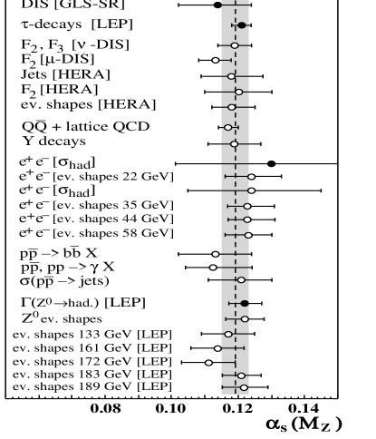
Figure 1: Compilation of $\alpha_{s}(M^{2}_{\rm Z})$ measurements. $\!{}^{{\bf?}}$

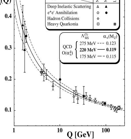
Figure 2: Running QCD coupling–1998. $\!{}^{{\bf?}}$

The results on $\alpha_{s}(M^{2}_{\rm Z})$ from $\!{}^{{\bf?},{\bf?},{\bf?}}$ are still preliminary. Table 1 and Fig. 1 display $\alpha_{s}(M^{2}_{\rm Z})$ results evolved using the 4-loop $\overline{\mbox{\scriptsize MS}}$ $\beta$-function with 3-loop matching $\!{}^{{\bf?}}$ at quark pole masses $M_{b}\!=$4.7 GeV and $M_{c}=$1.5 GeV. Fig. 2 collects $\alpha_{s}$ values at the proper scales of individual experiments and spectacularly demonstrates asymptotic freedom.

It is important to stress that “all meaningful subsamples of results provide similar average values, and there is no significant systematic shift between any of those subsamples”. Remarkedly, the “only $\rm e^{+}\rm e^{-}$” and “only DIS” subsamples peacefully coexist now, yielding $\alpha_{s}(M^{2}_{\rm Z})=$0.1210$\pm$0.0049 and $\alpha_{s}(M^{2}_{\rm Z})=$0.1175$\pm$0.0061 correspondingly. And so do “only $Q\leq$10 GeV” (0.1179$\pm$0.0043) and “only $Q\geq$30 GeV (0.1208$\pm$0.0058) measurements.

The world average value of the $\overline{\mbox{\scriptsize MS}}$ coupling $\alpha_{s}(M^{2}_{\rm Z})$ is finally quoted to be $\!{}^{{\bf?}}$

$$\alpha_{s}(M^{2}_{\rm Z})=0.119\pm 0.004\>.$$

This result is based on 18 (of 27) individual measurement from the Table 1 with the errors $\Delta\alpha_{s}(M^{2}_{\rm Z})\leq 0.008$. The overall uncertainty is derived by the “optimised correlation” method.$\!{}^{{\bf?}}$

1.3 $\alpha_{s}$ fresh from Lattice

A lattice analysis of the strong coupling was recently carried out by the group $\!{}^{{\bf?}}$ working on a QUADRICS QH1 at Orsay. Calculations were performed on $16^{4}$ and $24^{4}$ lattices with a bare lattice coupling constant $\beta\!=\!6$ (corresponding to an inverse lattice spacing $a^{-1}\simeq 1.9$ GeV). Calculations repeated for $\beta\!=\!6.2$ ($a^{-1}\simeq 2.7$ GeV) on a $24^{4}$ lattice (which roughly embodies the same physical volume as $16^{4}$ for $\beta\!=\!6.0$) yield consistent results. The primary objective of the study was to measure the coupling (Landau gauge, MOM subtraction scheme) “as defined in the text-books”. Namely,

1. to measure 3- and 2-point gluon correlations, the Green functions $G_{3}(p_{1},p_{2},-p_{1}-p_{2})$ and $G_{2}(p)=Z(p^{2})/p^{2}$,

2. truncate $G_{3}$ to extract the vertex function
   $\Gamma_{3}(p_{1},p_{2},p_{3})=G_{3}(p_{1},p_{2},p_{3})\prod_{i=1}^{3}G_{2}^{-1}(p_{i}^{2})$

3. and then construct the coupling at a symmetric Euclidean point $k^{2}\!>\!0$,

   $$\alpha_{s}(k^{2})=\left.\Gamma_{3}(p_{1},p_{2},p_{3})\right|_{p_{1}^{2}=p_{2}^{2}=p_{3}^{2}=-k^{2}}\cdot Z^{3/2}(-k^{2})\,.$$

Fig. 3 shows the result. The adjacent Fig. 4 displays the behaviour of a similar asymmetric correlator in which one of the three gluon momenta is set to zero.

Figure 3: Running coupling on the lattice.$\!{}^{{\bf?}}$

Figure 4: “Asymmetric” lattice coupling.$\!{}^{{\bf?}}$

The fact that the lattice coupling shows the tendency to decrease at small momenta should not surprise us. Regardless of which particular kind of confinement we observe on the lattice, the correlators of coloured fields had better vanish at the origin. The gluon Green function cannot have a pole at $p^{2}=0$, nor any similar singularity strong enough to propagate colour flux at large distances, $j(R)\cdot R^{2}={\cal{O}}\left(1\right)$. Therefore, having chosen to truncate $G_{3}$ with the text-book perturbative gluon propagators, we are bound to see $Z(p^{2})$ trying to kill the massless gluon pole.

It does not matter for our discussion how realistic these plots are. In particular, quarks were not included in the game. Even if they had been, there is always a question of how to incorporate light fermions with Compton wave lengths comparable to (exceeding) the volume of the lattice world. This is an especially troubling question if light quarks do indeed play a crucial rôle in the confinement of the world we live and experiment in.$\!{}^{{\bf?}}$

2 Measurements give rise to Assessments

2.1 The origin and status of $\alpha_{s}(k^{2})$

Therefore, those who are not thoroughly aware of the disadvantages in the use of arms cannot be thoroughly aware of the advantages in the use of arms.$\!{}^{{\bf?}}$

We are used to the notion of a running QCD coupling. What is its origin and status? Formally, $\alpha_{s}$ is a parameter of the perturbative expansion. From this point of view, its choice is, to a large extent, a matter of free will: it depends on how smart we want to be in organising the PT-series. It starts to make more sense, and becomes natural, within a programme of trading a formal expansion parameter for a smarter object, a momentum-dependent $\alpha_{s}(k^{2})$, which embodies some specific all-order radiative correction effects and is supposed to truly represent the interaction strength at a given momentum scale.

A bunch of questions immediately comes to mind:

• what high-order effects to embed?

• what does “truly represent” mean?

• what is the characteristic momentum scale that the running coupling depends on?

Renormalisability of the theory is known to be responsible for the running of the coupling. The Renormalisation Group tells us: “scale the whole World, and the answer remains the same provided $\alpha$ has been changed accordingly”. Stretching the World is not at our disposal, however. We may scale up/down external momenta but not, say, hadron masses. Therefore the running $\alpha_{s}$ rightfully appears in the realm of Hard Interactions characterised by a large momentum transfer, $Q^{2}\gg m^{2}$, and in the description of observables insensitive to finite InfraRed parameters (particle masses $m$).

The RG dictates how the renormalised coupling (constant) $\alpha_{s}(\mu_{R}^{2})$ changes with the renormalisation scale $\mu_{R}$. It is casually said that in small-distance amplitudes characterised by a single large Euclidean virtual momentum scale $Q\gg m$, the formal dependence on the renormalisation point, $\alpha_{s}(\mu_{R}^{2})$, can be traded for $\alpha_{s}(Q^{2})$ thus giving rise to the coupling (function) running with the physical momentum.

A couple of cautious comments are due before we go further. Firstly, trading $\alpha_{s}(\mu_{R}^{2})$ for $\alpha_{s}(Q^{2})$ implies that $\mu_{R}/Q$ is the only momentum ratio that enters. This is true for renormalised off-shell amplitudes. These are however unphysical and consequently gauge-dependent objects; hence, the problem of peeling off gauge-dependent effects from the running coupling. Dealing with “physical” gauge-independent on-shell amplitudes has a different problem. They are infrared sensitive and so have nasty $\alpha_{s}\ln Q/m$ (collinear) and $\alpha_{s}\ln Q/0$ (soft) high-order corrections. Therefore, one needs to treat collinear- and infrared-safe cross sections instead of $n$-point amplitudes.

Secondly, the way the running coupling emerges in Minkowskian observables is rather tricky. “On-shell” gluons are produced even from small distances $1/k\ll 1$ fm with a coupling $\alpha_{s}(0^{2})$, in a manner of speaking, and not with $\alpha_{s}(k^{2})$ (in a direct analogy with real photons from $Z$-peak being radiated with $\alpha_{em}(0)\simeq 1/137$ rather than $\alpha_{em}(M_{Z})\simeq 1/128$). What is instead determined by $\alpha_{s}(k^{2})$ is an intensity of inclusive emission of a gluon sub-jet with the total transverse momentum $k$ with respect to the radiating quark.

At the two-loop level the $\alpha_{s}(\mu_{R}^{2})$-dependence proves to be universal, i.e. independent of the choice of the PT-expansion parameter. This universality is inherited from the basic property of ultraviolet renormalisability of the theory. This part of the momentum variation of $\alpha_{s}$ is determined by the first two terms in the $\beta$-function,

$$\frac{d}{d\ln\mu_{R}}\left(\frac{\alpha_{s}(\mu_{R}^{2})}{2\pi}\right)^{-1}=\beta(\alpha_{s}(\mu_{R}^{2}))\>,$$

namely,

$$\beta(\alpha)\>=\>\beta_{0}+\beta_{1}\frac{\alpha}{2\pi}+\ldots$$

The further expansion terms $\beta_{n}$ with $n\geq 2$ remain scheme- (and even gauge)-dependent; in other words, arbitrary. Therefore, the large-momentum behaviour of the running coupling $\alpha_{s}(Q^{2})$ cannot be uniquely fixed beyond two loops. The reason for that is pretty simple: only the first two loops are truly dominated by the UV region, that is by small-distance physics.

There aren’t many UV-dominated QCD diagrams. Logarithmically divergent radiative corrections to gluon and quark wave functions (self energies) and to gluon-gluon (quark-gluon) interaction vertices are involved in the renormalisation of the coupling constant $\alpha_{s}$.

Consider for example a quark loop in the gluon self-energy. The one-loop radiative corrections contain the standard integral

$$\int\frac{d^{4}q}{q^{4}}\propto\ln\Lambda_{{\mbox{\scriptsize UV}}}\>\>=\>\>\infty\quad{\Longrightarrow}\quad\beta_{0}\>.$$

Hiding infinity under the carpet produces $\beta_{0}$, the first coefficient in the PT $\beta$-function expansion. In the next step we supply our quark loop with an additional internal gluon. Now we have two independent loop-momenta to integrate over, $q_{1}$ and $q_{2}$. Integration regions $q_{1(2)}\ll q_{2(1)}\ll\Lambda_{\mbox{\scriptsize UV}}$ could have produced $(\ln\Lambda_{\mbox{\scriptsize UV}})^{2}$ contributions. These get suppressed by renormalising the internal propagators and vertices at the one-loop level, the result being a single-logarithmic integral determined by the region $q_{1}\sim q_{2}\ll\Lambda_{\mbox{\scriptsize UV}}$,

$$\int\frac{d^{4}q}{q^{4}}\alpha_{s}(\mu_{R}^{2})\>\>\propto\>\>\alpha_{s}(\mu_{R}^{2})\ln\Lambda_{{\mbox{\scriptsize UV}}}\>\>=\>\>\infty\quad{\Longrightarrow}\quad\beta_{1}\>.$$ (1)

This is how the usual story goes, order by order in perturbation theory. We can do better, however, by taking into consideration that the coupling in (1) runs with the internal momentum. This means reorganising the PT series so as to incorporate into the two-loop diagram the higher order effects that result in substituting $\alpha_{s}(\mu_{R}^{2})\to\alpha_{s}(q^{2})$. By doing so we obtain a contribution which is still UV-divergent, though modified by the logarithmic decrease of the coupling at large momenta,

$$\int\frac{d^{4}q}{q^{4}}\alpha_{s}(q^{2})\propto\ln\ln\Lambda_{{\mbox{\scriptsize UV}}}\>\>=\>\>\infty\quad{\Longrightarrow}\quad\beta_{1}\>.$$

Renormalising it out gives rise to $\beta_{1}$. Starting from the third loop the situation however changes drastically: the UV-region is no longer dominant, and we get

$$\int\frac{d^{4}q}{q^{4}}\left(\alpha_{s}(q^{2})\right)^{2}\>\>=\>\>\mbox{finite}\quad{\Longrightarrow}\quad\mbox{\begin{minipage}{93.95122pt} $\beta_{n\geq 2}$ depend on the {\bf infrared} physics! \end{minipage}}$$

The notorious “nobody is perfect” applies to the above consideration as well. Strictly speaking, it is not known how to systematically refurbish, in all orders, the PT-series in terms of the running $\alpha_{s}$. So, this argument can be looked upon as yet another example of a statement “correct but unproven”,$\!{}^{{\bf?}}$ see however.$\!{}^{{\bf?}}$ Still, the message it sends is clear: starting from the $\alpha_{s}^{3}$ (next-to-next-leading) level, a purely perturbative treatment may become intrinsically ambiguous because of an interconnection between small and large distances. In particular, there may be no way of unambiguously defining the QCD coupling $\alpha_{s}$, beyond the two loops, without solving the Theory in the infrared.

2.2 Defining $\alpha_{s}$ beyond two loops

Bearing in mind this warning one can still attempt to define some PT expansion parameter $\alpha_{s}$ beyond two loops. To this end we may try different options.

1. As long as higher terms in the $\beta$-function are arbitrary anyway, why not simply set $\beta_{n\geq 2}\equiv 0$. This is the so-called ’t Hooft scheme which is perfectly fine but for one thing: the Landau singularity — the fake infrared problem — obviously limits the use of $\alpha_{s}$ so defined, to sufficiently large momentum scales.

2. One can design some sort of “optimisation principle” in order to fix $\beta_{2}$. The leading idea here is to minimise, one way or another, the effect of a (typically unknown, with few exceptions) three-loop PT correction to a given observable (Minimal Sensitivity, Fastest Apparent Convergence). Guided by sheer pragmatism (not necessarily a curse word) this approach often results in fixing $\beta_{2}$ such as to force $\alpha_{s}(k^{2})$ to develop a “spurious infrared fixed point”.

A (curse) word spurious appears here because the 3-loop $\beta$-function and the corresponding coupling that emerge from such an analysis are observable-dependent. Linked to this is a well-grounded criticism based on non-transitivity between the couplings defined on the base of different observables. Moreover, it is legitimate to ask ourselves, whether it makes sense to optimise PT series which are known to be senseless, factorially divergent, being contaminated by infrared renormalons.

Given all these reservations, it is still interesting to notice that such a “spuriously finite” coupling comes out close to the characteristic magnitude of the interaction strength in the infrared domain, the “couplant” $\left\langle\frac{\alpha_{s}}{\pi}\right\rangle\simeq 0.2$, which we shall discuss below.

3. We may try to link $\alpha_{s}$ with some physical quantity in a “most natural” way. To this family belong “effective charges”,$\!{}^{{\bf?}}$ specific, physically motivated, perturbative definitions of $\alpha_{s}$ such as, e.g., the BLM,$\!{}^{{\bf?}}$ CMW (MC),$\!{}^{{\bf?}}$ or Uraltsev $\!{}^{{\bf?}}$ schemes fitted to serve gluon exchange potential, relativistic gluon radiation and non-relativistic heavy quark physics, respectively. The words “most natural” don’t deceive us. Whether we like it or not, there is no direct link between $\alpha_{s}$ and observables, the latter being hadronic observables, in a confining theory.

4. It is perfectly allowable to play with the $\beta$-function (in particular, by adding to it non-analytic pieces) so as to make $\alpha_{s}(k^{2})$ freeze (or even vanish) in the origin. Everything is allowed as long as we do not spoil the large-momentum behaviour of the running $\alpha_{s}(k^{2})$ at the $1/\ln k$ and $(1/\ln k)^{2}$ level.

Rightfully rejecting the infrared “Landau singularity” in the coupling as being unphysical, or blaming infrared renormalons for spoiling PT expansions, or discussing possible links between $\alpha_{s}$ and hadronic observables we stumble upon the very same problem: what is a true measure of interaction between inexistent objects? By hook or by crook, the problem is that of defining the theory in the infrared: the confinement problem.

2.3 Does $\alpha_{s}$ at low momentum scales make sense?

Possible responses are

• Conservative: No way. It cannot be, because this can’t be, never.$\!{}^{{\bf?}}$ As long as there are no quarks and gluons in the physical spectrum of the theory, we cannot talk about the QCD interaction strength at distances above which colour-bearers get (mysteriously) confined. As a conservative position it is as impeccable as it is infertile.

• Liberal: Let’s try. Defining an infrared-finite coupling $\alpha_{s}$ may serve as a tool for probing universal features of colour confinement.$\!{}^{{\bf?}}$ (He who takes no risks drinks no champaign.)

• Revolutionary: We must. Dyson-Feynman’s is the only reliable Field-Theoretical language in our disposal. We have no other way but to employ quark and gluon Green functions down to $k\!=\!0$ and search for an unusual, confinement, solution.

Practically,

God has generously supplied us with light quarks capable of delivering early screening, preventing colour fields from going haywire. As shown by V.N. Gribov,$\!{}^{{\bf?}}$ to achieve super-critical binding of light quarks, and thus to ensure the screening of any colour fields, it suffices to have the average magnitude of the coupling in the InfraRed region as large as

$$\left\langle\frac{\alpha_{s}}{\pi}\right\rangle_{\mbox{{\mbox{\scriptsize{IR}}}}}>\frac{\alpha_{\mbox{\scriptsize crit}}}{\pi}\>=\>C_{F}^{-1}\left(1-\sqrt{2/3}\right)\>\simeq\>0.137\>.$$

The interesting thing about this number (apart from being easy to memorise) is that it is rather small.

Pragmatically,

if essential non-Abelian fields indeed grew really big, we would not even know how to properly define gluon degrees of freedom because of the notorious problem of “Gribov copies”.$\!{}^{{\bf?}}$ In Hamiltonian language, the Coulomb QCD interaction in the presence of transverse vacuum fields is described by the operator

$$D^{-1}=\partial^{2}\eta+g_{s}[{A_{\mu}^{\perp}},\partial_{\mu}\eta]\>,$$ (2)

reminiscent of the propagator of the Fadeev-Popov ghost in covariant gauges. In the second order in $g_{s}$, the statistical equal-time average of the product of two vacuum fields, $\left\langle A_{\mu}^{\perp}A_{\nu}^{\perp}\right\rangle\propto 4N_{c}$, takes over from the normal (unitary respecting) screening effect due to the splitting of the Coulomb gluon into “physical fields”, namely two transverse gluons ($-N_{c}/3$) or a $q\bar{q}$ pair ($-2n_{f}/3$).

This physical explanation of the anti-screening phenomenon,$\!{}^{{\bf?},{\bf?}}$ had a dramatic continuation. The normal magnitude of field fluctuations of spatial size $L$ is $LA^{\perp}(L)\sim 1$. In the background of very large vacuum fields, $LA^{\perp}(L)\sim g_{s}^{-1}$ (so large that the non-linearity becomes essential at the classical level), the Coulomb (ghost) propagator (2) becomes singular. Technically, this shows that we did not manage to properly define Lagrangian physical degrees of freedom, to divide out the volume of non-Abelian group transformations, to fix the gauge.

A chilling perspective of Fadeev-Popov ghosts rising from the dead makes one wish to get away with a numerically small coupling (relatively small fields) as a unique (and maybe only) chance to keep things under control.

Phenomenologically,

there is no sign of strong colour fields: confinement appears to be soft and friendly. There are three aspects to this friendliness:

1. pQCD works OK from very large scales down to $Q\!\!\sim$ 2 GeV, for the phenomena where it should (hadronic $\tau$-decays being an extreme example);

2. pQCD works down to (and below) $Q\sim$ 1–2 GeV where it did not have to (as it does, in particular, for DIS structure functions at HERA);

3. moreover, sometimes pQCD surprisingly works down to … $k\!\!=\!\!\mbox{\scriptsize NILL}$. This happens, notably, in describing inclusive energy and angular distributions of hadrons produced in hard processes, the phenomenon known as LPHD (local parton-hadron duality).$\!{}^{{\bf?},{\bf?}}$

What are the main lessons we have learned from experiment?

1. We have got used to pQCD covering orders of magnitude in the basic hard cross sections. More than that, our toddler-wisdom of how to estimate NP effects is being certified.

2. HERA tells us that proton is truly fragile. The transition from the $\gamma p$ physics to deep inelastic $\gamma^{*}p$ phenomena happens early, and it is sharp. The proton isn’t actually bound, if you take my meaning: a little scratch — and it is blown to pieces.

3. Finally, when viewed globally, confinement is about renaming a flying-away quark into a flying-away pion rather than about forces pulling quarks back together. From the study of numerous string/drag effects in particle flows, in $\rm e^{+}\rm e^{-}$ and at the Tevatron, we have learnt that even junky 200-300 MeV pions obediently follow the pattern of underlying colour fields. Whatever the ultimate solution of the confinement problem may be, it had better be gentle in transforming the quark-gluon Pointing-vector into the Pointing-vector of the final state hadrons.

2.4 Some like it perturbative

So, how to measure what we can’t define? The idea is to look for deviations of inclusive quantities that characterise hard processes, from their respective perturbative predictions. For a PT-calculable observable such a deviation, due to genuine NP (confinement) physics, is expected to be inverse proportional to a certain power of the hardness scale,

$$\frac{\delta\sigma^{\mbox{\scriptsize{NP}}}}{\sigma}\>\propto\frac{\log^{q}Q}{Q^{2p}}\>.$$

From within the PT-approach these (observable-dependent) powers can be inferred. Already at this stage we get a lot of valuable information. For example,

• we would have no chance to see one of the most precise determinations of $\alpha_{s}(M^{2}_{\rm Z})$ from the $\tau$-decay if confinement effects (which apriori could have been huge at as small a scale as $m_{\tau}<$ 2 GeV) were not strongly suppressed $\!{}^{{\bf?},{\bf?}}$ as $(\Lambda_{\mbox{\scriptsize QCD}}^{2}/m_{\tau}^{2})^{3}\ll 1$;

• an understanding of the leading NP power correction to the Drell–Yan $K$-factor,$\!{}^{{\bf?},{\bf?}}$ $1/Q^{2}$, calls for proper attention being paid to formulating the PT predictions for production of Drell–Yan lepton pairs, heavy flavours and high-invariant-mass jet pairs in hadronic collisions $\!{}^{{\bf?}}$ in order to avoid an artificial $1/Q$ contamination;$\!{}^{{\bf?}}$

• discriminating jet-shape variables according to the envisaged power of the leading NP contribution allows the selection of observables less affected by hadronisation and thus better suited for precise QCD tests such as measuring $\alpha_{s}$.

As we shall discuss below, jet shapes typically contain $1/Q$ NP contributions. Two examples of “cleaner” jet observables: the mean value of the three-jet resolution variable $y_{3}$, defined according to the Durham algorithm, which is hadronisation-sensitive at the $\log Q/Q^{2}$ level,$\!{}^{{\bf?}}$ or central moments,$\!{}^{{\bf?}}$ $\left\langle(V-\left\langle V\right\rangle)^{n}\right\rangle$, of most jet-shape observables $V$.

However the story does not end here. Not only can one trigger the exponent of the confinement contribution to a given observable but, making further assumptions, one may quantify the absolute magnitude of the NP effects by relating the deviations found for different observables.

The programme can be looked upon as pushing forward the Sterman-Weinberg wisdom. PT-calculable observables are Collinear-and-InfraRed-Safe (CIS) observables, those which can be calculated in terms of quarks and gluons without encountering either collinear (zero-mass quark, gluon) or soft (gluon) divergences. The procedure is straightforward.

1. Choose a CIS observable and get hold of the corresponding state-of-the-art PT-prediction;

2. enjoy the beauty of the latter;

3. observe that it has no sense (with $\alpha_{s}(k^{2})$ running through the “Landau pole”);

4. force it to have one (kindly ask $\alpha_{s}(k^{2})$ to behave);

5. as far as the PT prediction produces now a definite answer, given an IR-finite $\alpha_{s}$, see what you have done: quantify the ignorance about $\alpha_{s}$ in the low momentum range;

6. do it again for other observables;

7. verify that your ignorance is universal i.e. observable-independent;

8. eat your hat if it isn’t and switch to another business.

In recent years this programme has been carried out for a large set of practically interesting quantities including non-singlet DIS structure functions,$\!{}^{{\bf?},{\bf?},{\bf?}}$ $\rm e^{+}\rm e^{-}$ $\!{}^{{\bf?},{\bf?}}$ and DIS fragmentation functions,$\!{}^{{\bf?}}$ various jet shape characteristics (means and distributions in thrust, jet masses, $C$-parameter, jet broadening) in $\rm e^{+}\rm e^{-}$ annihilation $\!{}^{{\bf?},{\bf?},{\bf?},{\bf?},{\bf?}}$ and DIS,$\!{}^{{\bf?},{\bf?}}$ to heavy hadron spectra from heavy-quark-initiated jets $\!{}^{{\bf?}}$ and angular jet profiles.$\!{}^{{\bf?}}$ First encouraging steps have been made towards revealing the PT-NP interplay in hard small-$x$ phenomena such as high energy $\gamma^{*}\gamma^{*}$ scattering cross section,$\!{}^{{\bf?}}$ and non-singlet DIS structure functions.$\!{}^{{\bf?}}$

Among interesting confinement-sick quantities still queueing for treatment are back-to-back energy-energy correlation and transverse momentum spectra of Drell–Yan pairs (which should exhibit weird non-integer $Q$-exponents), out-of-event-plane characteristics of two- and three-jet events (such as $T_{minor}$ or oblateness), accompanying $E_{T}$ hadron flows in DIS and hadronic collisions, and many others.

3 Assessments give rise to Calculations

How to quantify NP corrections to hard observables? We shall sketch solutions to five major problems that arise on the way, namely

1. How to disentangle power corrections coming from UV and IR regions?

2. How to split the magnitude of the power term into an observable-dependent PT-calculable factor and a universal NP parameter?

3. Is the latter really universal? What is the accuracy of the universality statement?

4. How to merge PT and NP contributions to the full answer?

These being understood, the time comes to worry about your hat…

3.1 Problem # 1: IR vs UV

The trick of introducing small gluon mass $m$ into Feynman diagrams can be used to probe contributions of small momentum scales.$\!{}^{{\bf?},{\bf?},{\bf?},{\bf?},{\bf?}}$ Operationally, the procedure is quite simple. Consider the PT correction to a given observable $\sigma$, given by one-loop Feynman diagrams with one additional gluon, real or virtual. Real and virtual contributions, $\sigma_{r}$ and $\sigma_{v}$, are IR-sensitive. Introducing a finite mass into the Feynman propagator of the gluon regularises collinear and infrared divergences producing

$$\sigma_{r}\>,\>\>\sigma_{v}\>=\>{\cal{O}}\left(\ln^{2}\epsilon\right)+{\cal{O}}\left(\ln\epsilon\right)+{\cal{O}}\left(1\right)\>,\quad\epsilon\equiv\frac{m^{2}}{Q^{2}}\,.$$

However, having chosen a CIS observable we have secured the cancellation of divergent terms in the physical answer, so that

$$\sigma=\sigma_{r}\>+\>\sigma_{v}\quad=\quad{\cal{O}}\left(1\right)\,,$$

thanks to the Bloch-Nordsieck theorem. By examining, how fast does the $m$-dependent contribution to $\sigma$ vanish in the $\epsilon\to 0$ limit, we can quantify sensitivity of a given observable to large distances. To this end we have to look for contributions non-analytic in $\epsilon$ in the origin,$\!{}^{{\bf?},{\bf?},{\bf?},{\bf?}}$ while analytic corrections proportional to integer powers of $m^{2}/Q^{2}$ come from the UV momentum region, $k\sim Q$, in the Feynman integrals involving the modified gluon propagator,

$$G(k^{2})=\frac{1}{-k^{2}-i0}\>\Longrightarrow\>\frac{1}{m^{2}-k^{2}-i0}\,.$$ (3)

For example, the one-loop total $\rm e^{+}\rm e^{-}$ annihilation cross section into hadrons has the following structure,

$$\sigma=\sigma_{Born}\left(1+\frac{C_{F}\alpha_{s}}{2\pi}{\cal{R}}(\epsilon)\right),\quad{\cal{R}}(0)=\frac{3}{2}\>.$$

with ${\cal{R}}(\epsilon)$ the “characteristic function” for the $\sigma_{e^{+}e^{-}}$ depending on the gluon mass. Setting $\epsilon=0$ we recover the well-know first order PT correction $\sigma_{1}/\sigma_{Born}=\alpha_{s}/\pi$. The function ${\cal{R}}$ is known, and so is its small-$\epsilon$ behaviour,

$${\cal{R}}(\epsilon)=\frac{3}{2}-\frac{3}{2}\epsilon^{2}+\frac{11}{9}\epsilon^{3}-\frac{2\epsilon^{3}}{3}\ln\epsilon\>+\>{\cal{O}}\left(\epsilon^{4}\ln\epsilon\right).$$

This shows that all the ${\cal{O}}\left(\epsilon\right)$ terms present in $\sigma_{r}$ and $\sigma_{v}$ have cancelled in the sum, as well as the $\ln^{2}\epsilon$- and $\ln\epsilon$-enhanced ${\cal{O}}\left(\epsilon^{2}\right)$ corrections: non-analyticity starts at the ${\cal{O}}\left(\epsilon^{3}\right)$ level only. This property can be easily inferred from a mysterious reciprocity relation $\!{}^{{\bf?}}$ whose origin remains to be understood,

$${\cal{R}}(\epsilon)-\frac{3}{2}=\epsilon^{2}\left({\cal{R}}(\epsilon^{-1})-\frac{3}{2}\right).$$

The message that such a powerful extension of the Bloch-Nordsieck wisdom $\!{}^{{\bf?},{\bf?}}$ sends us is that the first genuine large-distance contribution to $\sigma_{e^{+}e^{-}}$ appears as a $Q^{-6}$ power correction, corresponding to the $\left\langle(\bar{\psi}\psi)^{2}\right\rangle$ vacuum condensate of dimension six, in the standard OPE language.$\!{}^{{\bf?},{\bf?}}$

We shall return to the issue of non-analyticity in $m^{2}$ a little later when we discuss the NP trigger. But first, a confession is due: the last thing one would like to do is to make the gluon field massive. Violating sacred non-Abelian gauge invariance eventually results in breaking the UV renormalisability of the theory.

Analytic coupling and “dispersive mass”.

Fortunately the situation is not so scary. What we actually need is not a real Lagrangian mass. It suffices to take into consideration the fact that the gluon, as any other quantum field, lives part-time in virtual states consisting of various parton configurations ($q\bar{q}$, $gg$, etc). These virtual transitions appear as a renormalisation of the gluon field,

$$G(k^{2})=\frac{1}{-k^{2}-i0}\>\Longrightarrow\>\frac{Z(k^{2})}{-k^{2}-i0}\>,$$ (4)

which can be characterised in terms of the distribution over “virtual mass” $m^{2}$ (gluon spectral function) via a dispersion relation. It is this mass that makes the gluon “heavy”.

The factor $Z$ has a simple physical meaning: it can be identified with the running coupling,

$$\frac{Z(-k^{2})}{Z(-\mu_{R}^{2})}\>=\>\frac{\alpha(k^{2})}{\alpha(\mu_{R}^{2})}\>,$$ (5)

with $\mu_{R}$ an arbitrary UV-renormalisation point. Such an identification is straightforward in the Abelian theory: in QED, due to the Ward identity, radiative corrections to the wave function of a charged particle (electron) and to the vertex cancel out ($Z_{1}=Z_{2}$); what remains is the photon propagator, $Z\equiv Z_{3}$. In QCD the gluon which mediates interaction between “charges” is a charged (coloured) particle itself. Therefore its wave function renormalisation, unlike that of the photon, is gauge-dependent and has no direct meaning. What then enters into the definition of the physical coupling is the gauge-invariant combination of the gluon propagator and specific non-Abelian corrections to the interaction vertices, which are independent of the nature (colour representation) of the external charges,

$$Z\>=\>\Gamma^{(\mbox{\scriptsize NA})}\cdot Z_{3}\cdot\Gamma^{(\mbox{\scriptsize NA})}\>.$$ (6)

Modulo this subtlety, in QCD we can still say that exchanging a gluon with 4-momentum $k$ brings in the propagator

$$G(k)\>=\>\frac{\alpha_{s}(-k^{2})}{-k^{2}-i0}$$ (7)

(where we have dropped an irrelevant overall constant). Now comes the crucial assumption: we want (7) to make sense in the entire complex $k^{2}$-plane. We know sufficiently well how $\alpha_{s}(-k^{2})$ behaves in the deep Euclidean region, at large negative $k^{2}$; we know next to nothing about small-$k^{2}$ region. However, whatever the function $\alpha_{s}$ is, it had better respect causality. Therefore we suppress the formal PT tachion (Landau singularity) and choose the “physical cut” alone, $0<k^{2}<\infty$, as a support for the dispersive relation,

$$\alpha_{s}(q^{2})=\int_{0}^{\infty}\frac{dm^{2}\>q^{2}}{(m^{2}+q^{2})^{2}}\,\alpha_{\mbox{\scriptsize eff}}(m^{2})\>.$$ (8)

Here $\alpha_{\mbox{\scriptsize eff}}$ is the dispersive companion of the standard coupling,

$$\frac{d}{d\ln\mu^{2}}\alpha_{\mbox{\scriptsize eff}}(\mu^{2})\>=\>-\frac{1}{2\pi i}\,\mbox{Disc}\left\{\alpha_{s}(-\mu^{2})\right\}.$$ (9)

The dispersion relation (8) can be formally inverted as the operator relation

$$\alpha_{\mbox{\scriptsize eff}}(\mu^{2})=\frac{\sin(\pi{\cal{P}})}{\pi{\cal{P}}}\,\alpha_{s}(\mu^{2})\>,\quad{\cal{P}}=\mu^{2}\frac{d}{d\mu^{2}}\>.$$ (10)

It shows that in the PT region $\alpha_{\mbox{\scriptsize eff}}$ and $\alpha_{s}$ are pretty close: $\alpha_{\mbox{\scriptsize eff}}(k^{2})=\alpha_{s}(k^{2})(1+{\cal{O}}\left(\alpha_{s}^{2}\right))$. One can design model expressions for $\alpha_{s}$ and the corresponding $\alpha_{\mbox{\scriptsize eff}}$. What matters in our discussion is that the latter gives us a direct hold on the large-distance contribution to the observable under study. We are ready for a “heavy gluon”. Substituting (8) into the gluon propagator (7) we can write

$$\frac{\alpha_{s}(-k^{2})}{-k^{2}-i0}=\int_{0}^{\infty}\frac{dm^{2}}{m^{2}}\,\alpha_{\mbox{\scriptsize eff}}(m^{2})\cdot\frac{-d}{d\ln m^{2}}\frac{1}{m^{2}-k^{2}-i0}\>.$$

Feynman diagrams contain an integration over the internal gluon momentum $d^{4}k$. We conclude that the answer can be represented as an $\alpha_{\mbox{\scriptsize eff}}(m^{2})$-weighted integral over the “mass” $m^{2}$ of the ($\ln m^{2}$–derivative of) the PT answer calculated by usual Feynman diagram techniques but with an as if massive gluon. Such a calculation produces an $m^{2}$-dependent characteristic function ${\cal{F}}_{V}$ specific to a given observable $V$. In the first order in the running coupling ${\cal{F}}$ is a function of $\epsilon=m^{2}/Q^{2}$ and is given by the one-loop diagrams with a gluon of mass equal to the dispersive variable, $0\leq m^{2}\leq\infty$. We get

$$V(Q^{2}\!\!,x)=\!\!\int_{0}^{\infty}\!\!\frac{dm^{2}}{m^{2}}\alpha_{\mbox{\scriptsize eff}}(m^{2})\dot{\cal{F}}_{V}(\epsilon,x);\>\>\dot{\cal{F}}\equiv\frac{-d{\cal{F}}}{d\ln\epsilon},$$ (11)

with $x$ a set of relevant dimensionless variables. At this point (11) is no different from the usual PT answer. The CIS nature of $V$ guarantees convergence of the $m^{2}$ integration: $\dot{\cal{F}}$ vanishes as a power of $\epsilon$ ($\epsilon^{-1}$) in the $\epsilon\to 0$ ($\epsilon\to\infty$) limit. Therefore the distribution $\dot{\cal{F}}_{V}(\epsilon)$ has a maximum at $\epsilon=C_{V}(x)={\cal{O}}\left(1\right)$, and the integral is dominated by the large-momentum region $m^{2}\sim Q^{2}$. Approximating $\alpha_{\mbox{\scriptsize eff}}(m^{2})\simeq\alpha_{s}(Q^{2})$ we easily reproduce the one-loop PT answer,

$$\sigma_{V}(Q^{2},x)\>\simeq\>\alpha_{s}(Q^{2}){\cal{F}}_{V}(0,x)\>.$$ (12)

Using the observable-dependent position of the maximum of the $m^{2}$-distribution as the scale for the coupling in (12), $\alpha_{s}(C_{V}(x)Q^{2})$, does a better job since it minimises higher order effects. In this respect the dispersive technology is closely related to the idea of “commensurate scales”.$\!{}^{{\bf?}}$

Renormalons.

We could have tried better still by taking into account PT corrections coming from logarithmic running of the coupling around the maximum. However there is an imminent danger around the corner. The deficiency of the PT series becomes apparent from the fact that the high-order expansion coefficients $R_{k}$ exhibit factorial growth.$\!{}^{{\bf?}}$ This is associated with both the UV and the IR integration regions in $\epsilon$.

At the one-loop level we can equate $\alpha_{\mbox{\scriptsize eff}}$ with $\alpha_{s}$ and substitute for $\alpha_{\mbox{\scriptsize eff}}(m^{2})$ the standard geometric series

$$\alpha_{\mbox{\scriptsize eff}}(m^{2})\simeq\alpha_{s}\sum_{k=0}^{\infty}\left(\frac{\beta_{0}\alpha_{s}}{4\pi}\;\ln\frac{Q^{2}}{m^{2}}\right)^{k}\!\!\!,\quad\alpha_{s}\equiv\alpha_{s}(Q^{2})\,.$$

This would give

$$V(Q^{2},x)-\alpha_{s}(Q^{2}){\cal{F}}_{V}(0,x)\>\simeq\>\alpha_{s}\sum_{k=1}^{\infty}\left(\frac{\beta_{0}\alpha_{s}}{4\pi}\right)^{k}\!\!R_{k}\,,$$

with the expansion coefficients given by

$$R_{k}=\int_{0}^{\infty}\frac{d\epsilon}{\epsilon}\left(\ln\frac{1}{\epsilon}\right)^{k}\dot{\cal{F}}_{V}(\epsilon)\,.$$ (13)

The ultraviolet contribution to $R_{k}$ is estimated by integrating (13) over $\epsilon>1$. If $\dot{\cal{F}}(\epsilon)$ vanishes as $\epsilon^{-q}$ at large $\epsilon$, one finds for large $k$

$$R_{k}^{{\mbox{\scriptsize UV}}}\sim\int_{1}^{\infty}\frac{d\epsilon}{\epsilon}\left(\ln\frac{1}{\epsilon}\right)^{k}\;\epsilon^{-q}\>\sim\>(-q)^{-k}\,k!\,.$$ (14)

This corresponds to an ultraviolet renormalon. Such an alternating series can be evaluated by Borel summation. This is because in the UV integration region the replacement $\alpha_{\mbox{\scriptsize eff}}(m^{2})\to\alpha_{s}(m^{2})$ is a reliable approximation and the contribution of this region can in fact be evaluated explicitly (e.g. numerically) without any expansion.

The infrared contribution to $R_{k}$ is estimated by integrating over the region $\epsilon<1$. The small-$\epsilon$ behaviour of the characteristic function can be cast as

$$\dot{\cal{F}}_{V}(\epsilon)\>\simeq\>\epsilon^{p}\>f_{V}(\ln\epsilon)\,,$$ (15)

with $f$ a polynomial at most quadratic in $\ln\epsilon$. Both the leading power $p$ and $f$ depend on the observable under consideration. Substituting into (13) one finds

$$R_{k}^{{\mbox{\scriptsize{IR}}}}=\int_{0}^{1}\frac{d\epsilon}{\epsilon}\left(\ln\frac{1}{\epsilon}\right)^{k}\;\epsilon^{p}\,f(\ln\epsilon)\>\sim\>p^{-k}\,k!$$ (16)

We again find a factorial behaviour known as an infrared renormalon. In this case however the coefficients are non-alternating and therefore the series is not Borel-summable. Attempts to ascribe meaning to such a series (which cannot even pretend at the status of asymptotic) give rise to unphysical complex contributions at the level of $Q^{-2p}$ terms. This is generally interpreted as an intrinsic uncertainty in the summation of the perturbative series. This problem is of a physical nature and cannot be resolved by formal mathematical manipulations alone. It requires genuinely new physical input to obtain a sensible answer.

3.2 Problem # 2: NP trigger

To extract the NP large-distance correction to a given observable we split the coupling into two components,

$$\alpha_{s}(k^{2})=\alpha^{\mbox{\scriptsize{PT}}}(k^{2})+\alpha^{\mbox{\scriptsize{NP}}}(k^{2})\>,$$

and use the latter as a trigger. It should be made clear that such a splitting is symbolic: it represents the coupling not in terms of two functions but rather of two procedures. This ambiguity will be dealt with later on. For the time being let us just sketch these two procedures.

• Having met $\alpha^{\mbox{\scriptsize{PT}}}(k^{2})$ under the integral we are advised to calculate it perturbatively, that is in terms of (not too long) a PT-series at the point $k^{2}\sim Q^{2}$ that our integral “sits” around. At the same time we are supposed not to worry about our PT-coupling being potentially sick in the IR momentum region.

• On the contrary, integrals with $\alpha^{\mbox{\scriptsize{NP}}}(k^{2})$ are believed to be determined by that very same IR region, below some finite few-GeV scale.

Since the integral of the type

$$\int_{0}^{\infty}\frac{dk^{2}}{k^{2}}\,\alpha_{s}^{\mbox{\scriptsize{NP}}}(k^{2})\cdot k^{2p}\>=\>\>\left(\mbox{few 100s MeV}\right)^{2p}$$ (17)

converges, it provides us with a dimensionful constant (analogous to the ITEP vacuum condensates$\!{}^{{\bf?}}$ for the OPE-controlled Euclidean quantities). These are the NP parameters that will determine the magnitude of $Q^{-2p}$-suppressed contributions to CIS observables.

As long as $\alpha_{s}^{\mbox{\scriptsize{NP}}}(k^{2})$ falls fast enough, its dispersive companion $\alpha_{\mbox{\scriptsize eff}}^{\mbox{\scriptsize{NP}}}(m^{2})$, according to (8), should have vanishing moments

$$\lim_{k\to\infty}k^{2p}\alpha^{\mbox{\scriptsize{NP}}}(k^{2})=0\>\Longleftrightarrow\>\int_{0}^{\infty}\frac{dm^{2}}{m^{2}}m^{2p}\alpha_{\mbox{\scriptsize eff}}^{\mbox{\scriptsize{NP}}}(m^{2})=0\,,$$

at least for the first few integer values of $p$. That is why substituting $\alpha_{\mbox{\scriptsize eff}}^{\mbox{\scriptsize{NP}}}$ for the full $\alpha_{\mbox{\scriptsize eff}}$ in (11) singles out specifically non-analytic terms in the characteristic function $\dot{\cal{F}}_{V}$. The leading non-analytic term in the $\epsilon\to 0$ behaviour of $\dot{\cal{F}}_{V}$ determines then the power $p$ of the $1/Q^{2p}$ NP contribution.

The usual view that the NP component of the coupling decays fast at large momenta is rooted in the standard ITEP-OPE ideology.$\!{}^{{\bf?}}$ According to the ITEP picture, NP physics is related to large-wavelength smooth gluon and quark fields. The presence of such fields in the vacuum does not affect the propagation of PT quanta with large Euclidean momenta, and $\alpha_{s}(k^{2})$ in the UV domain in particular. If those fields were non-singular at short distances, the quark and gluon propagators (and thus the running coupling) would be subject to exponentially small corrections only. Small-size instantons are believed to be the first (singular) non-trivial vacuum fields that disturb the propagation of quarks and gluons at the level of power corrections $k^{-2p}$ with large exponents $p>p_{\max}\sim\beta_{0}\sim 9$. Phenomenological victories of QCD sum rules are impressive.$\!{}^{{\bf?},{\bf?}}$ This does not necessarily mean however that the true separation between the UV and IR physics is indeed as sharp and deep as it is implied by the ITEP picture. A viable alternative could be that the gluon Green function at large momentum $k$, for example, bears the memory of the IR domain already at the level of the relative $k^{-4}$ term (the tail of the IR-singular gluon polarisation operator).$\!{}^{{\bf?}}$ Such a heretic proposal does not necessarily undermine the notion of the gluon condensate, $\left\langle\alpha_{s}G^{2}\right\rangle$. On the contrary, it can make it “calculable”.$\!{}^{{\bf?}}$ In what follows we shall concentrate on the practically most important smallest powers $p=\textstyle\frac{1}{2},1$ and leave to future disputes the intriguing question of the depth of the separation between the UV and IR phenomena.

The non-analyticity of $\dot{\cal{F}}$, necessary to generate NP power correction, is typically of two kinds. In the first case we have an integer power $\epsilon^{p}$ accompanied by logarithm(s) of $\epsilon$ which induces non-analyticity. This is the case of DIS structure functions, the Drell-Yan $K$-factor, the width of hadronic $\tau$-lepton decay and the total $\rm e^{+}\rm e^{-}$ annihilation cross section, etc. For example, for the valence DIS structure function one has

$$\lim_{m\to 0}\dot{\cal{F}}_{\mbox{\scriptsize DIS}}\>=\>a(x)\cdot\frac{m^{2}}{Q^{2}}\ln\frac{Q^{2}}{m^{2}}\quad+\ldots$$

Secondly, we may have a half-integer $p$. This is the case for many so-called jet-shape observables that characterise, in a CIS manner, the structure of final states produced in hard processes. Thrust, invariant jet masses, $C$-parameter, jet broadening, energy-energy correlation (as well as a list of others not yet being discussed in the literature) belong to the $p=\textstyle\frac{1}{2}$ class. These quantities should embody $1/Q$ power effects due to confinement physics:$\!{}^{{\bf?},{\bf?}}$

$$\lim_{m\to 0}\dot{\cal{F}}_{V}\>=\>{a_{V}}\cdot\sqrt{\frac{m^{2}}{Q^{2}}}\quad+\ldots$$

Thrust.

Historically the first among the jet shapes addressed in this context has been the thrust, which measures the “pencilness” of the final state system,

$$T=\max_{\vec{n}}\frac{\sum_{i}|\vec{n}\cdot\vec{p}_{i}|}{\sum_{i}|\vec{p}_{i}|}\>.$$

The direction $\vec{n}$ that maximises $T$ is called the thrust axis. Two back-to-back particles with 4-momenta $p$ and $\bar{p}$ (or clusters of particles with parallel momenta) produced in the centre of mass of $\rm e^{+}\rm e^{-}$ annihilation with cms energy $Q$ correspond to $T\!=\!1$. Thrust deviates from unity for two reasons. One is PT gluon bremsstrahlung. $T$ is obviously a CIS observable since neither collinear parton splitting nor infinitely soft gluon radiation affect its value. Therefore the PT-component of the mean thrust is

$$\left\langle 1-T\right\rangle^{(\mbox{\scriptsize{PT}})}\>=\>{\cal{O}}\left(\alpha_{s}\right)\>.$$ (18)

Another reason is pure hadronisation physics. pQCD radiation being switched off, two outgoing quarks are believed to produce two narrow jets of hadrons which are uniformly distributed in rapidity and have limited transverse momenta with respect to the jet axis (Field-Feynman hot-dog, or a string). Within a simplified “tube model” with an exponential inclusive distribution of hadrons

$$\frac{dN}{d\eta dk_{\perp}}=\mu^{-1}\>\vartheta(\eta_{m}-|\eta|)\>e^{-k_{\perp}/\mu}\>,\quad\mu=\left\langle k_{\perp}\right\rangle\>,$$

we have

$$\sum_{i}|\vec{p}_{i}| = 2\!\!\int\!d\eta\,dk_{\perp}\frac{dN}{d\eta dk_{\perp}}\>k_{\perp}\cosh\eta=2\mu\sinh\eta_{m}=Q\,;$$

$$\sum_{i}|p_{zi}| = 2\!\!\int\!d\eta\,dk_{\perp}\frac{dN}{d\eta dk_{\perp}}\>k_{\perp}\sinh\eta=2\mu(\cosh\eta_{m}-1)\,,$$

where, for the sake of simplicity, we have treated hadrons as massless. Constructing the ratio we obtain

$$T=\frac{\cosh\eta_{m}-1}{\sinh\eta_{m}}=1-\frac{2\mu}{Q}+{\cal{O}}\left(\frac{\mu^{2}}{Q^{2}}\right),$$

so that the departure of thrust from unity occurs at the $1/Q$ level, with the characteristic hadronisation transverse momentum as a relevant scale,

$$\left\langle 1-T\right\rangle^{(\mbox{\scriptsize{NP}})}\simeq\frac{2\left\langle k_{\perp}\right\rangle}{Q}\>.$$ (19)

Introducing finite hadron mass(es) does not change the result. It is from the study of hadronisation models that the $1/Q$ effects first came into focus.$\!{}^{{\bf?}}$

The PT approach normally would not provide us with such a dimensionful parameter: gluon transverse momenta are broadly (logarithmically) distributed which results in the mean $\left\langle k_{\perp}\right\rangle\propto\alpha_{s}Q$, in accord with (18).

However now we have a PT-handle on the large-distance physics, thanks to the “gluon-mass” trigger. Contribution to thrust from a single gluon with momentum $k$ reads, in terms of light-cone (Sudakov) variables, $k=\alpha p+\beta\bar{p}+{\bf k}_{\perp}$,

$$\delta(1-T)\>=\>{\min\{\alpha,\beta\}}\>.$$

Calculating the characteristic function for $\left\langle 1-T\right\rangle$ one obtains

$${\cal{F}}_{T} \simeq \frac{C_{F}}{\pi}\int\frac{d\alpha}{\alpha}\frac{d\beta}{\beta}dk_{\perp}^{2}\delta(\alpha\beta Q^{2}-k_{\perp}^{2}-m^{2})\cdot{\min\{\alpha,\beta\}}$$

$$= \frac{2C_{F}}{\pi\,Q}\int_{0}^{Q^{2}}\frac{dk_{\perp}^{2}}{\sqrt{k_{\perp}^{2}+m^{2}}}\>.$$

Hence,

$$\dot{\cal{F}}\equiv-m^{2}\frac{d\,{\cal{F}}}{dm^{2}}\simeq\frac{2C_{F}}{\pi}\>\frac{m}{Q}\>,$$

which is precisely the $\sqrt{m^{2}}$ non-analyticity we were expecting. It is easy to see that the leading non-analyticity is due to the radiation of soft gluons at large angles, $k_{0}\sim k_{\perp}\sim m\ll Q$.

Since soft gluon radiation has in fact a classical nature and its pattern is simple, as it is universal, the relative magnitudes of the NP contributions to CIS jet shapes appear to be simple as well. For example, for the mean jet shapes one obtains

$$\left\langle V\right\rangle^{\mbox{\scriptsize{NP}}}=\frac{a_{V}}{Q}\cdot\frac{C_{F}}{2\pi}\int_{0}^{\infty}\frac{dm^{2}}{m^{2}}\sqrt{m^{2}}\>\alpha_{\mbox{\scriptsize eff}}^{\mbox{\scriptsize{NP}}}(m^{2})\>,$$ (20)

where the coefficients $a_{V}$ are simple numbers having a clear geometric origin.

3.3 Problem # 3: Universality

The very concept of the IR-finite coupling would make no sense without universality, i.e. if we had to introduce for each observable a private phenomenological parameter to fix the magnitude of the confinement contribution. Therefore it is natural that the universality concept has been intensively argued for.$\!{}^{{\bf?},{\bf?},{\bf?}}$

It was soon recognised, however, that the technologies based on the “massive gluon” trigger, whether the renormalon-motivated approach tracing the series of fermion bubbles or the dispersive approach, are intrinsically ambiguous since there is no unique prescription for including finite-$m^{2}$ effects into the definition of the shape variable. For example, a perfectly legitimate definition of thrust for a 3-parton system that consists of massless $q\bar{q}$ and a massive gluon, suggested by Beneke and Braun, has produced a result differing by a factor $\simeq 1.8$ from the “conventional” (20).$\!{}^{{\bf?}}$ The “naive estimate” that emerges as a result of substituting a “massive gluon” for the real final-state system of massless partons is fine for triggering the power of the NP-contribution but fails to predict its magnitude, the latter remaining prescription-dependent.

Moreover, as has been already mentioned above, the running $\alpha_{s}(k^{2})$ in Minkowskian observables emerges only at the inclusive level, as a result of an integration over positive virtualities of the gluon decaying into final-state offspring partons. Nason and Seymour rightfully questioned the application of the inclusive treatment of gluon decays. They pointed out that jet shapes are not truly inclusive observables, since kinematics of the offspring matters for the $V$ value. Therefore the configuration of offspring partons in the gluon decay may affect the value of the power term at next-to-leading level in $\alpha_{s}$, which a priori is no longer a small parameter since the characteristic momentum scale is low.

Both these problems called for analysis of the NP-effects at the two-loop level. Such analysis has been performed, and the result came out unexpectedly simple. It was shown that there exists a definite prescription for defining the “naive estimate” of the magnitude of the power contribution, such that the two-loop effects of non-inclusiveness of jet shapes reduce to a universal, observable-independent, renormalisation of the “naive” answer by the factor $\!{}^{{\bf?}}$

$${\cal{M}}\>\simeq\>1.76\>\>{(1.67)}\quad\mbox{for}\>\>n_{f}=3\>\>{(0)}\,.$$

This is true for the NP-effects in the thrust, invariant jet mass, $C$-parameter and broadening distributions. The same factor (known as the Milan factor) also applies to the energy-energy correlation measure away from the back-to-back region as well as to the linear jet-shape observables in DIS.$\!{}^{{\bf?}}$

The universality of the Milan factor has three ingredients. Firstly, it relies on the universality of soft radiation, the latter being responsible for confinement effects. Secondly, it obviously incorporates the concept of the universal the QCD interaction strength, all the way down to small momentum scales (which has been processed through the dispersive machinery). Finally, it stems from a certain geometric universality of the observables under consideration, which includes their linearity, collinear finiteness (convergence of rapidity integrals) and Lorentz invariance (independence of the gluon decay matrix element on the parent gluon rapidity).$\!{}^{{\bf?}}$

Strictly speaking, the accuracy of the Milan factor isn’t great: the next loop would bring in the correction

$${\cal{M}}^{\mbox{true}}={\cal{M}}^{{\mbox{2-loop}}}\left(1+{\cal{O}}\left(\frac{\alpha_{s}}{\pi}\right)\right)$$

with $\alpha_{s}$ entering at small scale. Hence, a $\sim 20\%$ uncertainty in the value of the ${\cal{M}}$ factor cannot be excluded. At the same time, the above ingredients of its universality seem to be general enough as to ensure its validity even beyond two loops.

3.4 Problem # 4: Merging

We agreed to treat $\alpha_{s}^{\mbox{\scriptsize{NP}}}$ as a procedure rather than a function, and thus representing the NP-component of the answer in the form (20) is not the end of the story. It is unsatisfactory in two respects. Psychologically, it does not satisfy our curiosity about interaction strength. More importantly, it remains symbolic since its PT-counterpart is given by a renormalon-sick series. We need to marry the PT and NP components into a reasonable answer. To this end we first trade $\alpha_{\mbox{\scriptsize eff}}$ back for the standard coupling by invoking the identity following from (8),

$$\int_{0}^{\infty}\frac{dm^{2}}{m^{2}}\,m\,\alpha_{\mbox{\scriptsize eff}}^{\mbox{\scriptsize{NP}}}(m^{2})={\frac{4}{\pi}}\cdot\int_{0}^{\infty}dk\>\alpha^{\mbox{\scriptsize{NP}}}(k^{2})\>.$$

Then, we truncate the integration at some arbitrary finite value $\mu_{I}$ which is large enough to neglect the NP interaction, $\alpha_{s}^{\mbox{\scriptsize{NP}}}(k)\simeq 0$, $k>\mu_{I}$, and get rid of $\alpha_{s}^{\mbox{\scriptsize{NP}}}$ by substituting

$$I=\int_{0}^{\mu_{I}}dk\>\alpha^{\mbox{\scriptsize{NP}}}(k^{2})=\int_{0}^{\mu_{I}}dk\>\alpha_{s}(k^{2})-\int_{0}^{\mu_{I}}dk\>\alpha^{\mbox{\scriptsize{PT}}}(k^{2})\,.$$

The first integral quantifies the average interaction strength in the IR, via

$${\alpha}_{0}(\mu_{I})\>\equiv\>\frac{1}{\mu_{I}}\int_{0}^{\mu_{I}}dk\>\alpha_{s}(k^{2}).$$

The second contribution should be calculated perturbatively, as a series in $\alpha_{s}$. The series for this subtraction term is factorially divergent in high orders, as is the basic series for $\left\langle V\right\rangle^{\mbox{\scriptsize{PT}}}$. Introduction of the IR matching scale $\mu_{I}$ makes the full combined answer renormalon-free though. Finally,

$$\left\langle V\right\rangle=\left\langle V\right\rangle^{\mbox{\scriptsize{PT}}}(\alpha_{s})+a_{V}\cdot{\cal{P}}\>,$$ (21)

where the universal NP parameter ${\cal{P}}\sim 1/Q$ equals, to the second order in $\alpha_{s}$,

$${\cal{P}}\> = \>\left.\frac{4C_{F}{\cal{M}}}{\pi^{2}}\frac{\mu_{I}}{Q}\cdot\right\{{\alpha}_{0}(\mu_{I})$$ (22)

$$\left.-\left[\,\alpha_{s}+\beta_{0}\frac{\alpha_{s}^{2}}{2\pi}\left(\ln\frac{Q}{\mu_{I}}+1+{\frac{K}{\beta_{0}}}\right)+\ldots\right]\right\}$$

Here $K$ is a known number depending on the scheme chosen for the PT expansion parameter $\alpha_{s}=\alpha_{s}(Q^{2})$. A residual $\mu_{I}$-dependence, at the level of ${\cal{O}}\left(\alpha_{s}^{3}\mu_{I}/Q\right)$, is the price for having a renormalon-free answer. In principle it can be reduced by continuing the PT-series, both for $\left\langle V\right\rangle^{\mbox{\scriptsize{PT}}}$ and the subtraction in (22). The coefficients $a_{V}$ in (21) for mean thrust, $C$-parameter and invariant total and heavy-jet masses in $\rm e^{+}\rm e^{-}$ annihilation are

$$\begin{array}[]{|l|c||c||c|c|}\hline\cr V=&\>1-T&\>\>C&\>M_{T}^{2}&\>M^{2}_{H}\\ \hline\cr a_{V}=&2&3\pi&2&1\\ \hline\cr\end{array}$$ (23)

The same NP-parameter (21) that governs the leading confinement effect in the means affects the jet-shape distributions as well. In the “soft” kinematical region $\Lambda_{\mbox{\scriptsize QCD}}/Q\ll V\ll V_{\max}$ it reveals itself as a shift in the pure perturbative spectrum,$\!{}^{{\bf?},{\bf?}}$

$$\frac{d\sigma}{dV}(V)\>=\>\frac{d\sigma^{(\mbox{\scriptsize{PT}})}}{dV}(V-a_{V}{\cal{P}})\>.$$ (24)

The phenomenology of $1/Q$ effects in jet-shape means and distributions suggests

$${\cal{A}}_{1}\equiv\frac{C_{F}}{2\pi}\int_{0}^{\infty}\frac{dk^{2}}{k^{2}}\cdot k\>\alpha_{s}^{\mbox{\scriptsize{NP}}}(k^{2})\>\simeq\>0.2\mbox{--}0.25\,\mbox{GeV}\,.$$

Leading power corrections to other observables are determined by higher moments of $\alpha^{\mbox{\scriptsize{NP}}}$. In particular, studies of $1/Q^{2}$ power corrections to DIS structure functions allow the quantification of the second moment of the NP-coupling, corresponding to $p=1$ in (17),$\!{}^{{\bf?},{\bf?}}$

$${\cal{A}}_{2}\equiv\frac{C_{F}}{2\pi}\int_{0}^{\infty}\frac{dk^{2}}{k^{2}}\cdot k^{2}\>\alpha_{s}^{\mbox{\scriptsize{NP}}}(k^{2})\>\sim\>0.2\,\mbox{GeV}^{2}.$$

Dedicated discussions of different aspects of what we know, think we know and think about $\alpha_{s}$ can be found in the literature. Among the most recent are: OPE, duality and the “physical coupling”,$\!{}^{{\bf?}}$ the simplest model for the IR-finite $\alpha_{s}$,$\!{}^{{\bf?}}$ a more sophisticated model which fits two known moments, $p\!=\!\textstyle\frac{1}{2}$ and $p\!=\!1$, and respects OPE,$\!{}^{{\bf?}}$ discussion of the causality issue,$\!{}^{{\bf?}}$ instructive lessons about OPE, IR-finite coupling and the Landau pole from the $O(N)$ $\sigma$-model.$\!{}^{{\bf?}}$

4 Calculations give rise to Comparisons

The phenomenology of power-suppressed contributions to jet shapes had a vibrant but somewhat troubled childhood. Only thrust and $C$-parameter remained unaffected by theoretical misconceptions (some of which we are going to sort out below).

A ball-park value of $\alpha_{0}\simeq 0.5$ was repeatedly emerging from the analyses of jet shapes in $\rm e^{+}\rm e^{-}$ and DIS current jets in the Breit frame.$\!{}^{{\bf?},{\bf?},{\bf?},{\bf?},{\bf?}}$ A typical resume of 1997 would run like “The concept of a ‘universal’ Power Correction parameter $\alpha_{0}$ in DIS $ep$ scattering and $\rm e^{+}\rm e^{-}$ annihilation is supported”.$\!{}^{{\bf?}}$ However the same H1 group was the first to complain about the expected $\ln Q$ enhancement of the $1/Q$ correction to broadening $\!{}^{{\bf?}}$ which was inconsistent with experiment. The puzzle was recently put under scrutiny and clarified by the resurrected JADE collaboration. A detailed analysis presented at the Montpellier QCD conference by Pedro Movilla Fernandez showed that hadronisation effects in broadening not only shift the distribution to larger $B$ values (as it is the case for $1\!-\!T$ and $C$) but also squeeze it. As a consequence, fitting the data with a $\log Q$-enhanced $B$-independent shift yields inconsistent results for the total and wide-jet broadening distributions (marked “old $B_{T}$” and “old $B_{W}$” in Fig. 5). They are also far away, in the parameter space, from the consistent pair of the thrust and $C$-parameter distributions (solid $T$ and $C$ ellipses in Fig. 5).$\!{}^{{\bf?}}$ Alarming experimental conclusions “inconsistent results for jet broadening variables” and “effective coupling moments incompatible with each other” (read: there is no universality) made theoreticians jump on the train and revisit the problem from their side.

Figure 5: 95% CL contours for jet shape means (dashed) and some distributions (solid).

It was soon recognised that one essential phenomenon was overlooked in the original NP-treatment of broadening,$\!{}^{{\bf?}}$ namely an interplay between NP- and PT-phenomena. To put it short, the effects produced by NP-radiation in the presence of normal PT-radiation are different from the effects of NP-radiation inferred from a pure first-order analysis, that is when the PT-radiation is “switched off”.

NP-effects in the presence of PT-radiation.

It is not for the first time that such “mistake” has been made. There is a whole list of confusions that came from the first-order analysis disregarding normal ever-present PT-gluons.

The story of the heavy-jet mass is the simplest example. As you may remember from the previous discussion, to trigger the NP-contribution we are advised to add to the parton system a soft gluer,$\!{}^{{\bf?}}$ a gluon with $k_{\perp}\sim m\sim\Lambda_{\mbox{\scriptsize QCD}}$. Let us do so at the Born level, that is add a gluer to the $q\bar{q}$ system as the third and only secondary parton. Constructing $M^{2}$ of the quark-gluer system we will find a $1/Q$ confinement contribution to the squared mass of the heavy jet, the one our gluer belongs to. Meanwhile, the opposite lighter jet containing a lonely quark gets none of it. As a result the NP-correction to $M^{2}_{H}$ came out equal to that for thrust,

$$a_{T}=a_{M^{2}_{T}}=a_{M^{2}_{H}}\,,\quad a_{M^{2}_{L}}=0\>.\qquad\qquad\mbox{(wrong)}$$ (25)

In reality there are always normal PT gluons in the game which are responsible for the bulk of the jet mass: $M^{2}_{H}/Q^{2}\sim\alpha_{s}>M^{2}_{L}/Q^{2}\sim\alpha_{s}^{2}\gg\delta M^{2}_{\mbox{\scriptsize{NP}}}$. In these circumstances it is not gluer’s business to decide which of the jets is going to be heavier. Confinement effects are instead shared equally, see (23),

$$a_{T}=a_{M^{2}_{T}}=2a_{M^{2}_{H}}=2a_{M^{2}_{L}}\>.\qquad\qquad\mbox{(right)}$$ (26)

It is worthwhile noticing that experimental analyses carried out before 1998 were based on the wrong expectation (25), which is obviously not the experimenters’ fault.

Another still popular “mistake” is to expect that the NP-contributions to jet shapes can be suppressed by measuring higher moments, for example, $\left\langle(1\!-\!T)^{n}\right\rangle$. The one-gluon analysis indeed would formally produce for such an observable

$$\left\langle(1\!-\!T)^{n}\right\rangle_{\mbox{\mbox{\scriptsize{NP}}\ only}}\>\>\simeq\>\frac{{\cal{A}}_{n}}{Q^{n}}.$$

However what we are dealing with in reality instead is

$$(1\!-\!T)^{n}=\left[\,(1\!-\!T)_{\mbox{\scriptsize{PT}}}+(1\!-\!T)_{\mbox{\scriptsize{NP}}}\,\right]^{n}.$$

Symbolically,

$$\left\langle\left((1\!-\!T)_{\mbox{\scriptsize{PT}}}+\frac{\Lambda_{\mbox{\scriptsize QCD}}}{Q}\right)^{\!\!n}\right\rangle\simeq\alpha_{s}+\alpha_{s}\frac{\Lambda_{\mbox{\scriptsize QCD}}}{Q}+\ldots\left(\frac{\Lambda_{\mbox{\scriptsize QCD}}}{Q}\right)^{\!\!n}\!\!\!.$$

The leading $1/Q$ contribution is still here, reduced by the $\alpha_{s}(Q^{2})$ factor but far more important than the $1/Q^{n}$ term.

Another “mistake” of this sort brings us closer to the $B$-issue. Consider the transverse momentum broadening of the current-fragmentation jet in DIS, that is the sum of moduli of transverse momenta of particles in the current jet. Adding a gluer to the Born (parton model) quark scattering picture we get three equal contributions to $B$: two contributions from the quark $p$ which recoils against the gluer $k$ emitted either in the initial (IS) or in the final (FS) state, $|\vec{p}_{\perp}|=|\vec{k}_{\perp}|$, and one contribution from the gluer itself when it belongs to FS. Taking into account the PT-radiation, however, the FS quark has already got a non-zero transverse momentum, $\rm p_{\perp}^{\mbox{\scriptsize{PT}}}\sim\alpha_{s}\cdot Q$, a substantial amount compared to $k_{\perp}\sim\Lambda_{\mbox{\scriptsize QCD}}$. In this environment the direct gluer’s contribution is the only one to survive: the NP-recoil upon the quark gets degraded down to the $1/Q^{2}$ effect after the azimuthal average is performed,

$$\left\langle|\vec{p}_{\perp}|\right\rangle=\left\langle|\vec{p}_{\perp}^{\>\mbox{\scriptsize{PT}}}-\vec{k}_{\perp}|\right\rangle=p_{\perp}^{\mbox{\scriptsize{PT}}}+{\cal{O}}\left(\frac{\Lambda_{\mbox{\scriptsize QCD}}^{2}}{p_{\perp}^{\mbox{\scriptsize{PT}}}}\right).$$

The true magnitude of the $1/Q$ contribution turns out to be a factor three smaller than that extracted from the one-gluon analysis.

Now we are ready to address the squeezed broadening issue.$\!{}^{{\bf?}}$

The feature that $1\!-\!T$ and $C$ have in common is that the dominant NP-contribution to these and similar shapes is determined by radiation of gluers at large angles. This radiation is insensitive to the tiny mismatch, $\Theta_{q}={\cal{O}}\left(\alpha_{s}\right)$, between the quark and thrust axis directions which is due to PT gluon radiation. Therefore the quark momentum direction can be identified with the thrust axis.

The broadening, on the contrary, accumulates contributions which do not depend on rapidity, so that the mismatch between the quark and the thrust axis starts to matter both in the $B$-means and distributions.

If one naively assumes that the quark direction coincides with that of the thrust axis, then $B$ accumulates NP-contributions from gluers $i$ with rapidities up to the kinematically allowed value $\eta_{i}\leq\eta_{\max}\simeq\ln(Q/k_{ti})$. In this case one finds the shift in the $B$-spectrum to be logarithmically enhanced,

$$\Delta_{B}\>=\>a_{B}{\cal{P}}\cdot\ln\frac{Q}{Q_{B}}\>,$$ (27)

where $a_{B}=1(\textstyle\frac{1}{2})$ for the total (single-jet; wide-jet) broadening.$\!{}^{{\bf?}}$ What was overlooked here is the fact that the uniform distribution in $\eta_{i}$ (defined with respect to the thrust axis) holds only for rapidities not exceeding $|\ln\Theta_{q}|$. High-energy gluers with $k_{0i}>k_{ti}/\Theta_{q}$ are collinear to the quark direction rather than to that of the thrust axis and therefore do not contribute essentially to $B$. As a result, the NP-contribution to $B$ comes out proportional to the quark rapidity,

$$\delta B_{1}^{(\mbox{\scriptsize{NP}})}\>\simeq\>a_{1}{\cal{P}}\cdot\ln\frac{1}{\Theta_{q}}\>.$$ (28)

How does this affect NP-contributions to $\left\langle B\right\rangle$ and to the $B$-distributions? The power correction to the mean single jet broadening $\left\langle B\right\rangle_{1}$ is obtained by evaluating the perturbative average of $\delta B_{1}$ in (28),

$$\left\langle\delta B\right\rangle_{1}^{(\mbox{\scriptsize{NP}})}\>\simeq\>a_{1}{\cal{P}}\cdot\left\langle\ln\frac{1}{\Theta_{q}}\right\rangle.$$ (29)

At the Born level, the PT-distribution in the quark angle $\Theta_{q}$ is singular at $\Theta_{q}\!=\!0$. In high orders this singularity is damped by the double-logarithmic Sudakov form factor. As a result, the NP-component of $\left\langle B\right\rangle_{1}$ gets enhanced by

$$\left\langle\ln\frac{1}{\Theta_{q}}\right\rangle\>\simeq\>\frac{\pi}{2\sqrt{C_{F}\alpha_{s}(Q)}}\>.$$ (30)

For the mean wide jet broadening $\left\langle B\right\rangle_{W}$ the result has the same structure with the replacement $C_{F}\to 2C_{F}$ due to the fact that now it is radiation off two jets which determines the $\Theta_{q}$ distribution.

The shift in the single jet (wide jet) broadening can be expressed as

$$\Delta_{1}(B)\>\simeq\>a_{1}{\cal{P}}\cdot\left\langle\ln\frac{1}{\Theta_{q}}\right\rangle_{B}\>,$$ (31)

where the average is performed over the perturbative distribution in the quark angle $\Theta_{q}$ while keeping the value of $B$ fixed. Since $\Theta_{q}$ is kinematically proportional to $B$, the $\log$-enhancement of the shift in the $B$-spectrum becomes

$$\Delta_{1}(B)\>\simeq\>a_{1}{\cal{P}}\cdot\ln\frac{B_{0}}{B}$$ (32)

(with $B_{0}$ a calculable function slowly dependent on $\alpha_{s}\ln B$. Thus, the shift in the $B_{1}$ ($B_{W}$) distribution becomes logarithmically dependent on $B$.

The shift in the total two-jet broadening distribution $\Delta_{T}(B)$ has a somewhat more complicated $B$-dependence. In the kinematical region where the multiplicity of gluon radiation is small, $\alpha_{s}\ln^{2}B\ll 1$, one of the two jets is responsible for the whole PT-component of the event broadening, while the second is “empty”. That “empty” jet contributes the most to the shift: in the absence of perturbative radiation the direction of the quark momentum in this jet stays closer to the thrust axis. This results in

$$\Delta_{T}(B)\>\simeq\>\Delta_{1}(B)+\left\langle B\right\rangle_{1}^{(\mbox{\scriptsize{NP}})}\>\simeq\>a_{1}{\cal{P}}\left(\ln\frac{1}{B}+\frac{\pi}{2\sqrt{C_{F}\alpha_{s}}}\right).$$

In these circumstances the $B$-dependence of the total shift practically coincides with that of a single jet. In the opposite regime of well developed PT-radiation, $\alpha_{s}\ln^{2}B\gg 1$, the jets are forced to share $B$ equally, and we have instead

$$\Delta_{T}(B)\>\simeq\>2\cdot\Delta_{1}(B/2)\simeq 2\cdot a_{1}{\cal{P}}\>\ln\frac{1}{B}\,.$$

It is the $\log B$-enhancement of the NP shift that makes the final distribution narrower than its PT-counterpart.

On July 27${}^{\mbox{\scriptsize th}}$ when this talk was being delivered, the origin of the “mistake” was already clear but the true answer still unknown. Therefore it wasn’t risk-free to bet that the $B$-distributions would eventually agree with respectable $T$ and $C$. Fig. 5, which is preliminary, shows $95\%$ CL contours for $\alpha_{s}(M^{2}_{\rm Z})$ and $\alpha_{0}$ as extracted from $B_{T}$ distributions in the energy range 35–183 GeV, and also from the mean values of $C$, $T$, $M_{H}^{2}$, $B_{T}$ and $B_{W}$. Some care is to be taken in interpreting these results, since no account has been taken of the correlation of systematic errors.$\!{}^{{\bf?}}$

The universality of confinement effects has moved on to firmer ground, and with it, the concept of an IR-finite coupling.

5 Comparisons give rise to Victories

In our pursuit of confinement effects we were following the logic of the great Chinese warrior-philosopher Master Sun Tzu who said:

The rules of the military are five: measurement, assessment, calculation, comparison and victory. The ground gives rise to measurements, measurements give rise to assessments, assessments give rise to calculations, calculations give rise to comparisons, comparisons give rise to victories.$\!{}^{{\bf?}}$

In our context, it would be a bit premature to talk about victories yet. It will suffice to have noticed that

• QCD is alive and remains a rich source of technical and conceptual theoretical problems, of experimental challenges and phenomenological amusement;

• things are orderly in the “Hard Domain”, and $\alpha_{s}(Q^{2})$ among them;

• a crazy idea of probing perturbatively the “Soft Domain” has gained ground;

• the pQCD-motivated technology for triggering and quantifying, in a universal way, genuine confinement effects in hard observables is under construction,

• and that the effective large-distance interaction strength inferred from these studies, ${\left\langle\frac{\alpha_{s}}{\pi}\right\rangle_{\mbox{{\mbox{\scriptsize{IR}}}}}\simeq 0.14-0.17}$, turns out to be sufficiently small as to apply PT-language, at least semi-quantitatively, down to small momentum scales.

According to my assessment, even if you have many more troops than others, how can that help you to victory? $\!{}^{{\bf?}}$

Heat is building up, and QCD is about to undergo a faith transition: we are getting ready to convince ourselves to talk about “quarks and gluons” down to, and into, the InfraRed. This is the core of the Gribov programme of attacking the colour confinement.$\!{}^{{\bf?}}$ It is interesting to remark that the average IR coupling, though numerically rather small, appears at the same time to be just large enough to activate the super-critical light-quark confinement mechanism. Is it a mere coincidence? Could be. To answer the question, the last Gribov works should be understood and developed (the write-up of the second paper concluding his two-decade QCD study remained unfinished). This won’t be easy, given the complexity of the problem and, sadly, stone-solidness of our prejudice.

When on surrounded ground, plot.
When on deadly ground, fight.$\!{}^{{\bf?}}$

It is worth to keep in mind that on the QCD ground, as we know it today, to fight isn’t enough. To plot is often necessary. There is hardly a theorem around for which a proof could be concluded by the respectable QED = Quod Erat Demonstrandum (what had to be shown). The abbreviation QCD suits more, Quod Convenit Demonstrandum (what was agreed to be shown). A call for imagination and intuition, and guts to defend them, is what singles out the QCD island of the SM archipelago, the island where you never get bored.

References

References

- [1] Yu.L. Dokshitzer, hep-ph/9801372.
- [2] V.N. Gribov, “QCD at large and short distances”, hep-ph/9807224 (Annotated version of hep-ph/9708424); “The theory of quark confinement”, Bonn preprint TK 98-09, Dec 1998; Lund preprint LU 91–7 (1991); Physica Scripta T 15, 164 (1987).
- [3] P. Nason and C. Oleari, Nucl. Phys. B 521, 237 (1998) [hep-ph/9709360]; G. Rodrigo, Nucl. Phys. Proc. Suppl. 54A, 60 (1997); G. Rodrigo, A. Santamaria and M. Bilenkii, Phys. Rev. Lett. 79, 193 (1997); W. Bernreuther, A. Brandenburg and P. Uwer, Nucl. Phys. Proc. Suppl. 64, 387 (1998) [hep-ph/9709282] ; ibid. 65, 39 (1998) [hep-ph/9709281].
- [4] S. Catani, M. H. Seymour, Invited talk at Cracow International Symposium on Radiative Corrections (CRAD 96), Cracow, Poland, Aug 1996, Acta Phys.Polon. B 28, 863 (1997) [hep-ph/9612236]; Nucl. Phys. B 485, 291-419 (1997), Erratum-ibid. B 510, 503 (1997) [hep-ph/9605323]; Z. Bern, L. Dixon, D.C. Dunbar, D.A. Kosower, Talk given at 5 International Workshop on Deep Inelastic Scattering and QCD, Chicago, Apr 1997 [hep-ph/9706447].
-
[5]
S. Catani, M.L. Mangano, P. Nason and L. Trentadue,
Phys. Lett. B 378, 329 (1996);
R. Bonciani, S. Catani, M. L. Mangano and P. Nason, Nucl. Phys. B 529, 424 (1998) [hep-ph/9801375]; M. Cacciari, M. Greco and P. Nason, JHEP 05, 007 (1998) [hep-ph/9803400]. - [6] S. Catani, M. L. Mangano and P. Nason, JHEP 07, 024 (1998) [hep-ph/9806484].
- [7] D.J. Miller and M. H. Seymour Phys. Lett. B 435, 213 (1998) [hep-ph/9805414].
- [8] S. Catani and B.R. Webber, Phys. Lett. B 427, 377 (1998) [hep-ph/9801350].
- [9] Yu.L. Dokshitzer, A. Lucenti, G. Marchesini and G.P. Salam, JHEP 01, 011 (1998) [hep-ph/9801324].
- [10] Z. Bern, J.S. Rozowsky, B. Yan, Phys. Lett. B 401, 273 (1997) [hep-ph/9702424]; Z. Bern, V. Del Duca, C.R. Schmidt, hep-ph/9810409.
- [11] L.N. Lipatov, Sov. J. Nucl. Phys. 23, 338 (1976); E.A. Kuraev, L.N. Lipatov and V.S. Fadin, Sov. Phys. JETP 45, 199 (1977); Ya. Balitskii and L.N. Lipatov, Sov. J. Nucl. Phys. 28, 822 (1978).
- [12] V.S. Fadin and L.N. Lipatov, [hep-ph/9802290]; M. Ciafaloni and G. Camici, [hep-ph/9803389], Phys. Lett. B 412, 396 (1997) [hep-ph/9707390]; M. Ciafaloni, Phys. Lett. B 429, 363 (1998) [hep-ph/9801322].
- [13] B. Andersson, G. Gustafson and J. Samuelsson, Nucl. Phys. B 467, 443 (1996).
- [14] G. Camici and M. Ciafaloni, Phys. Lett. B 395, 118 (1997) [hep-ph/9612235]; Yu.V. Kovchegov and A.H. Mueller, [hep-ph/9805208]; E.M. Levin, [hep-ph/9806228]; N. Armesto, J. Bartels and M.A. Braun, hep-ph/9808340.
- [15] G. Bottazzi, G. Marchesini, G.P. Salam and M. Scorletti, hep-ph/9810546 and references therein.
- [16] M. Ciafaloni and G. Camici, Nucl. Phys. B 496, 305 (1997) [hep-ph/9701303]; G. Salam, JHEP 07, 019 (1998) [hep-ph/9806482].
- [17] A.V. Radyushkin, Phys. Lett. B 385 (1996) 333; Phys. Rev. D 56 (1997) 5524.
- [18] X. Ji, Phys. Rev. Lett. 78, 610 (1997); Phys. Rev. D 55, 7114 (1997).
- [19] A.V. Radyushkin, Phys. Lett. B 380, 417 (1996); P.A.M. Guichon and M. Vanderhaeghen, Prog. Part. Nucl. Phys. 41, 125 (1998) [hep-ph/9806305].
- [20] J. C. Collins, L. Frankfurt and M. Strikman, Phys.Rev. D 56 (1997) 2982; M. Diehl, T. Gousset, B. Pire and J. Ralston, Phys. Lett. B 411, 193 (1997); A.D. Martin and M.G. Ryskin, PRD 57, 6692 (1998) [hep-ph/9711371]; L. Mankiewicz, G. Piller and T. Weigl, Eur.Phys.J. C 5, 119 (1998).
- [21] I.I. Balitsky and A. V. Radyushkin, Phys. Lett. B 413, 114 (1997); J. Blumlein, B. Geyer and D. Robaschik,Phys. Lett. B 406, 161 (1997).
- [22] X. Ji and J. Osborne, Phys. Rev. D 58, 094018 (1998); A.V. Radyushkin, Phys. Rev. D 58, 114008 (1998).
- [23] S.J. Brodsky and P. Hoyer, Phys. Lett. B 298, 165 (1993); M. Luo, J.W. Qiu and G. Sterman, Phys. Rev. D 50, 1951 (1994); M. Gyulassy and X.-N. Wang, Nucl. Phys. B 420, 583 (1994); R. Baier, Yu. L. Dokshitzer, A. H. Mueller and D. Schiff, hep-ph/9804212 and references therein; B.G. Zakharov, Phys. Atom. Nucl. 61, 838 (1998) [hep-ph/9807540] and references therein; B.Z. Kopeliovich, A.V. Tarasov and A. Schafer, hep-ph/9808378.
- [24] S. Bethke, Presented at the IV Intern. Symp. on Radiative Corrections, Barcelona, Sept 8-12, 1998.
- [25] S. Bethke, Nucl. Phys. Proc. Suppl. 64, 54 (1998) [hep-ex/9710030].
- [26] J.H. Kim et al., Phys. Rev. Lett. 81, 3595 (1998).
- [27] R. Barate et al., ALEPH collab., Eur. Phys. J. C 4, 409 (1998).
- [28] K. Ackerstaff et al., OPAL collab., CERN-EP/98-102.
- [29] C. Adloff et al., H1 collab., Eur. Phys. J. C 5, 265 (1998); DESY 98-087, hep-ex/9807019.
- [30] M. Jamin and A. Pich, hep-ph/9709495.
- [31] R. Ammar et al., CLEO collab., Phys. Rev. D 57, 1350 (1998) [hep-ex/9707018].
- [32] P. A. Movilla Fern ndez, O. Biebel and S. Bethke, paper contributed to this Conference, hep-ex/9807007.
- [33] M. Grünewald, D. Karlen, contributions to this Conference.
- [34] L3 collab., CERN-EP/98-148; LEP papers contributed to this Conference.
- [35] K.G. Chetyrkin et al., hep-ph/9706430.
- [36] M. Schmelling, Phys. Scripta 51, 676 (1995).
- [37] Ph. Boucaud, F. Di Renzo, J. Micheli, J.P. Leroy, C. Parrinello, O. Pene, C. Pittori, C. Roiesnel, private communication.
- [38] Master Sun Tzu, ca 6 century BC, cited from: The illustrated Art of War by Sun Tzu; translated by Thomas Cleary, Shambhala, Boston & London, 1998.
- [39] Leonard Euler, Opera Omnia.
- [40] N.J. Watson, NPB 494, 388 (1997) [hep-ph/9606381]
- [41] G. Grunberg, Phys. Rev. D 29, 2315 (1984); ibid. 46, 2228 (1992); J. M. Campbell, E. W. N. Glover and C. J. Maxwell, Phys. Rev. Lett. 81, 1568 (1998) [hep-ph/9803254].
- [42] S.J. Brodsky, G.P. Lepage and P.B. Mackenzie, Phys. Rev. D 28, 228 (1983); T. Appelquist, M. Dien and I. Muzinich, Phys. Rev. D 17, 2074 (1978); M. Peter, Phys. Rev. Lett. 78, 602 (1997) [hep-ph/9702245].
- [43] S. Catani, G. Marchesini and B.R. Webber, Nucl. Phys. B 349, 635 (1991); S. Catani and L. Trentadue, Nucl. Phys. B 327, 323 (1989).
- [44] N.G. Uraltsev, Nucl. Phys. B 491, 303 (1997); A. Czarnecki, K. Melnikov and N. Uraltsev, Phys. Rev. Lett. 80, 3189 (1998) [hep-ph/9708372].
- [45] Late 19 century philosopher Koz’ma Prutkoff. Published.
- [46] A.C. Mattingley and P.M. Stevenson, Phys. Rev. D 49, 437 (1994).
- [47] V.N. Gribov, Nucl. Phys. B 139, 1 (1978).
- [48] I.B. Khriplovich, Yad. Fiz. 10, 409 (1969) [Sov. J. Nucl. Phys. 10, 235 (1970)].
- [49] Yu.L. Dokshitzer and S.I. Troyan, “Asymptotic freedom and local parton-hadron duality”, in: Proc. of XIX LNPI Winter School, Leningrad, 1984; Yu.L. Dokshitzer, V.A. Khoze, A.H. Mueller and S.I. Troyan, Basics of Perturbative QCD, ed. J. Tran Thanh Van, Editions Frontières, Gif-sur-Yvette, 1991.
- [50] for recent review see V.A. Khoze and W. Ochs, Int. J. Mod. Phys. A 12, 2949 (1997).
- [51] E. Braaten, S. Narison and A.Pich, Nucl. Phys. B 373, 58 (1992); A. Pich, Nucl. Phys. Proc. Suppl. 39, 326 (1995); G. Altarelli, P. Nason and G. Ridolfi, Z. Phys. C 68, 257 (1995); M. Neubert, Nucl. Phys. B 463, 511 (1996) [hep-ph/9509432].
- [52] P. Ball, M. Beneke and V.M. Braun, Nucl. Phys. B 452, 563 (1995) [hep-ph/9502300].
- [53] M. Beneke and V.M. Braun, Nucl. Phys. B 454, 253 (1995).
- [54] R. Akhoury, L. Stodolsky and V.I. Zakharov, Nucl. Phys. B 516, 317 (1998) [hep-ph/9609368] and references therein.
- [55] S. Catani, M.L. Mangano, P. Nason and L. Trentadue, Nucl. Phys. B 478, 273 (1996) [hep-ph/9604351].
- [56] E.L. Berger and H. Contopanagos, Phys. Rev. D 54, 3085,3113 (1996) [hep-ph/9603326].
- [57] Yu.L. Dokshitzer, G. Marchesini and B.R. Webber, Nucl. Phys. B 469, 93 (1996) [hep-ph/9512336].
- [58] B.R. Webber, Talk at 27th International Symposium on Multiparticle Dynamics (ISMD 97), Frascati, Italy, Sep 1997, Nucl. Phys. Proc. Suppl., 71, 66 (1999) [hep-ph/9712236].
- [59] M. Dasgupta and B.R. Webber, Phys. Lett. B 382, 273 (1996) [hep-ph/9604388].
- [60] E. Stein, M. Meyer-Hermann, L. Mankiewicz and A. Schäfer, Phys. Lett. B 376, 177 (1996) [hep-ph/9601356]; M. Meyer-Hermann et al., Phys. Lett. B 383, 463 (1996) [hep-ph/9605229], ibid. 393, 487 (1997) (E); M. Maul, E. Stein, A. Schäfer and L. Mankiewicz, Phys. Lett. B 401, 100 (1997) [hep-ph/9612300]; M. Maul et al., hep-ph/9710392; M. Meyer-Hermann and A. Schäfer, hep-ph/9709349.
- [61] B.R. Webber, Phys. Lett. B 339, 148 (1994); see also Proc. Summer School on Hadronic Aspects of Collider Physics, Zuoz, Switzerland, August 1994, ed. M.P. Locher (PSI, Villigen, 1994) [hep-ph/9411384].
- [62] M. Dasgupta and B.R. Webber, Nucl. Phys. B 484, 247 (1997) [hep-ph/9608394]; P. Nason and B.R. Webber, Phys. Lett. B 395, 355 (1997) [hep-ph/9612353]; M. Beneke, V.M. Braun and L. Magnea, Nucl. Phys. B 497, 297 (1997) [hep-ph/9701309].
- [63] M. Dasgupta, G.E. Smye and B.R. Webber, JHEP 04, 017 (1998) [hep-ph/9803382].
- [64] G.P. Korchemsky and G. Sterman, Nucl. Phys. B 437, 415 (1995) [hep-ph/9411211].
- [65] A.V. Manohar and M.B. Wise, Phys. Lett. B 344, 407 (1995) [hep-ph/9406392]; Yu.L. Dokshitzer and B.R. Webber, Phys. Lett. B 352, 451 (1995) [hep-ph/9504219]; G.P. Korchemsky, G. Oderda and G. Sterman, in Deep Inelastic Scattering and QCD, 5 International Workshop, Chicago, IL, April 1997, p. 988 [hep-ph/9708346]; R. Akhoury and V.I. Zakharov, Phys. Lett. B 357, 646 (1995) [hep-ph/9504248]; Nucl. Phys. B 465, 295 (1996) [hep-ph/9507253].
- [66] P. Nason and M.H. Seymour, Nucl. Phys. B 454, 291 (1995) [hep-ph/9506317].
- [67] Yu.L. Dokshitzer and B.R. Webber, Phys. Lett. B 404, 321 (1997) [hep-ph/9704298].
- [68] Yu.L. Dokshitzer, A. Lucenti, G. Marchesini and G.P. Salam, Nucl. Phys. B 511, 396 (1998) [hep-ph/9707532]; JHEP 05, 003 (1998) [hep-ph/9802381].
- [69] B.R. Webber, in: Workshop on DIS and QCD, Paris, 1995, ed. J.F.Laporte and Y. Sirois, p. 115.
- [70] M. Dasgupta and B.R. Webber, Eur. Phys. J. C 1, 539 (1998) [hep-ph/9704297]; JHEP 10, 001 (1998) [hep-ph/9809247].
- [71] Yu.L. Dokshitzer, V.A. Khoze and S.I. Troyan, Phys. Rev. D 53, 89 (1996) [hep-ph/9506425]; P. Nason and B.R. Webber, Phys. Lett. B 395, 355 (1997) [hep-ph/9612353].
- [72] W.T. Giele, E.W.N. Glover, D.A. Kosower, Phys. Rev. D 57, 1878 (1998) [hep-ph/9706210]; M. Seymour, Nucl. Phys. B 513, 269 (1998) [hep-ph/9707338].
- [73] F. Hautmann, Phys. Rev. Lett. 80, 3198 (1998) [hep-ph/9710256]
- [74] E. Stein, M. Maul, L. Mankiewicz and A. Schafer, hep-ph/9803342; G.E. Smye, hep-ph/9810292.
- [75] M. Beneke, V.M. Braun and V.I. Zakharov, Phys. Rev. Lett. 73, 3058 (1994).
- [76] M. Beneke and V.M. Braun, PLB 348, 513 (1995).
- [77] K. Wilson, Phys. Rev. D 179, 1499 (1969).
- [78] M.A. Shifman, A.I. Vainstein and V.I. Zakharov, Nucl. Phys. B 147, 385, 448, 519 (1979).
- [79] S.J. Brodsky and H.J. Lu, Talk at International Symposium on Heavy Flavor and Electroweak Theory, Beijing, P.R. China, Aug 1995. Published in Beijing Heavy Flavor 1995:0001-24, hep-ph/9601301; S.J. Brodsky, Talk at Workshop on Future Directions in Quark Nuclear Physics, Adelaide, Australia, Mar 1998, hep-ph/9806445; S.J. Brodsky et al., Phys. Rev. D 56, 6980 (1997) [hep-ph/9706467].
- [80] For recent reviews and classical references see V.I. Zakharov, Nucl. Phys. B 385, 452 (1992); A.H. Mueller, in QCD 20 Years Later, vol. 1 (World Scientific, Singapore, 1993); M. Beneke, hep-ph/9807443.
- [81] M.A. Shifman, in: QCD, 20 years later, ed. P.M Zerwas and H.A. Kastrup, World Scientific, 1993: v. 2, p. 775.
- [82] Vacuum Structure and QCD Sum Rules: Reprints, ed. M.A. Shifman, North-Holland, 1992: Current Physics, Sources and Comments, v. 10.
- [83] G. Grunberg, hep-ph/9807494.
- [84] H. Contopanagos and G. Sterman, Nucl. Phys. B 419, 77 (1994); G.P. Korchemsky and G. Sterman, in Proc. 30 Rencontres de Moriond, Meribel les Allues, France, March 1995, hep-ph/9505391.
- [85] G.P. Korchemsky, hep-ph/9806537.
- [86] B. Chibisov, R.D. Dikeman, M. Shifman, and N.G. Uraltsev, Int. J. Mod. Phys. A 12, 2075 (1997) [hep-ph/9605465].
- [87] D.V. Shirkov and I.L. Solovtsov, Phys. Rev. Lett. 79, 1209 (1997) [hep-ph/9704333].
- [88] B.R. Webber, JHEP 10, 012 (1998) [hep-ph/9805484].
- [89] E. Gardi, G. Grunberg and M. Karliner, JHEP 07, 007 (1998) [hep-ph/9806462].
- [90] M. Beneke, V.M. Braun and N. Kivel, hep-ph/9809287.
- [91] O. Biebel, Nucl. Phys. Proc. Suppl. 64, 22 (1998) [hep-ex/9708036]; D. Wicke, ibid. 64, 27 (1998) [hep-ph/9708467].
- [92] ALEPH collab., International Europhysics Conference on High-Energy Physics, Jerusalem, Israel, Aug 1997, contribution # 610; J. C. Thompson (ALEPH collaboration), contribution to this Conference, hep-ex/9812004.
- [93] C. Adloff et al., H1 collab., Phys. Lett. B 406, 256 (1997) [hep-ex/9706002].
- [94] H1 collab., contribution to this Conference, # 530.
- [95] P. A. Movilla Fernandez, talk at QCD Euroconference, Montpellier, France, July 1998, hep-ex/9808005.
- [96] Milan collab., Dec. 1998, under preparation.
- [97] G. Salam, private communication.