BEYOND THE STANDARD MODEL FOR HILLWALKERS

Abstract

In the first lecture, the Standard Model is reviewed, with the aim of seeing how its successes constrain possible extensions, the significance of the apparently low Higgs mass indicated by precision electroweak experiments is discussed, and defects of the Standard Model are examined. The second lecture includes a general discussion of the electroweak vacuum and an introduction to supersymmetry, motivated by the gauge hierarchy problem. In the third lecture, the phenomenology of supersymmetric models is discussed in more detail, with emphasis on the information provided by LEP data. The fourth lecture introduces Grand Unified Theories, with emphases on general principles and on neutrino masses and mixing. Finally, the last lecture contains short discussions of some further topics, including supersymmetry breaking, gauge-mediated messenger models, supergravity, strings and $M$ phenomenology.

1 GETTING MOTIVATED

There have been many reviews of different subjects in particle physics ‘for pedestrians’. At this school many of us had the fun experience of walking in the Scottish hills, which is more strenuous than a stroll across the Old Course at St Andrews, though less dangerous than mountain climbing in the Alps. The spirit of these lectures is similar: an invigorating introduction to modern phenomenological trends, but not too close to the theoretical precipices.

1.1 Recap of the Standard Model

The Standard Model  continues to survive all experimental tests at accelerators. However, despite its tremendous successes, no-one finds the Standard Model [1] satisfactory, and many present and future experiments are being aimed at some of the Big Issues raised by the Standard Model : is there a Higgs boson? is there supersymmetry? why are there only six quarks and six leptons? what is the origin of flavour mixing and CP violation? can the different interactions be unified? does the proton decay? are there neutrino masses? For the first time, clear evidence for new physics beyond the Standard Model  may be emerging from non-accelerator neutrino physics [2]. Nevertheless the Standard Model remains the rock on which our quest for new physics must be built, so let us start by reviewing its basic features and examine whether its successes offer any hint of the direction in which to search for new physics.

We first review the electroweak gauge bosons and the Higgs mechanism of spontaneous symmetry breaking by which we believe they acquire masses [3]. The gauge bosons are described by the action

$${\cal L}=-\frac{1}{4}~{}G^{i}_{\mu\nu}G^{i\mu\nu}-{1\over 4}F_{\mu\nu}F^{\mu\nu}$$ (1)

where $G^{i}_{\mu\nu}\equiv\partial_{\mu}W^{i}_{\nu}-\partial_{\nu}W^{i}_{\mu}+ig\epsilon_{ijk}W^{j}_{\mu}W^{k}_{\nu}$ is the field strength for the $SU(2)$ gauge boson $W^{i}_{\mu}$, and $F_{\mu\nu}\equiv\partial_{\mu}W^{i}_{\nu}-\partial_{\nu}W^{i}_{\mu}$ is the field strength for the $U(1)$ gauge boson $B_{\mu}$. The action (1) contains bilinear terms that yield the boson propagators, and also trilinear and quartic gauge-boson interactions. The gauge bosons couple to quarks and leptons via

$${\cal L}_{F}=-\sum_{f}i~{}~{}\left[\bar{f}_{L}\gamma^{\mu}D_{\mu}f_{L}+\bar{f}_{R}\gamma^{\mu}D_{\mu}f_{R}\right]$$ (2)

where the $D_{\mu}$ are covariant derivatives:

$$D_{\mu}\equiv\partial_{\mu}-i~{}g~{}\sigma_{i}~{}W^{i}_{\mu}-i~{}g^{\prime}~{}Y~{}B_{\mu}$$ (3)

The $SU(2)$ piece appears only for the left-handed fermions $f_{L}$, which are isospin doublets, while the right-handed fermions $f_{R}$ are isospin singlets, and hence couple only to the $U(1)$ gauge boson $B_{\mu}$, via hypercharges $Y$.

The origin of all the masses in the Standard Model  is an isodoublet scalar Higgs field, whose kinetic term in the action is

$${\cal L}_{\phi}=-|D_{\mu}\phi|^{2}$$ (4)

and which has the magic potential:

$${\cal L}_{V}=-V(\phi):V(\phi)=-\mu^{2}\phi^{\dagger}\phi+{\lambda\over 2}(\phi^{\dagger}\phi)^{2}$$ (5)

Because of the negative sign for the quadratic term in (5), the symmetric solution $<0|\phi|0>=0$ is unstable, and if $\lambda>0$ the favoured solution has a non-zero vacuum expectation value which we may write in the form:

$$<0|\phi|0>=<0|\phi^{\dagger}|0>=v\left(\matrix{0\cr{1\over\sqrt{2}}}\right):v^{2}={\mu^{2}\over 2\lambda}$$ (6)

corresponding to spontaneous breakdown of the electroweak gauge symmetry.

Expanding around the vacuum: $\phi=<0|\phi|0>+\,\hat{\phi}$, the kinetic term (4) for the Higgs field yields mass terms for the gauge bosons:

$${\cal L}_{\phi}\ni-{g^{2}v^{2}\over 2}~{}~{}W^{+}_{\mu}~{}W^{\mu-}-g^{\prime 2}~{}{v^{2}\over 2}~{}B_{\mu}~{}B^{\mu}+g~{}g^{\prime}v^{2}~{}B_{\mu}~{}W^{\mu 3}-g^{2}~{}{v^{2}\over 2}~{}W^{3}_{\mu}~{}W^{\mu 3}$$ (7)

There are also bilinear derivative couplings of the gauge bosons to the massless Goldstone bosons $\eta$, e.g., in the charged-boson sector we have

$$-\partial_{\mu}~{}\eta^{+}~{}\partial_{\mu}~{}\eta^{-}+~{}\left({igv\over 2}\partial_{\mu}~{}\eta^{+}~{}W^{\mu-}+h.c.\right)$$ (8)

Combining these with the first term in (7), we see a quadratic mass term for the combination

$$W^{+}_{\mu}-2i~{}~{}{\partial_{\mu}~{}\eta^{+}\over gv}$$ (9)

of charged bosons. This clearly gives a mass to the $W^{\pm}$ bosons:

$$m_{W^{\pm}}={gv\over 2}$$ (10)

whilst the neutral gauge bosons $(W^{3}_{\mu},B_{\mu})$ have a 2$\times$2 mass-squared matrix:

$$\left(\matrix{{g^{2}\over 2}&{-gg^{\prime}\over 2}\cr\cr{-gg^{\prime}\over 2}&{g^{\prime 2}\over 2}}\right)v^{2}$$ (11)

This is easily diagonalized to yield the mass eigenstates:

$$Z_{\mu}={gW^{3}_{\mu}-g^{\prime}B_{\mu}\over\sqrt{g^{2}+g^{\prime 2}}}~{}:~{}~{}m_{Z}={1\over 2}\sqrt{g^{2}+g^{\prime 2}}v~{};~{}~{}A_{\mu}={g^{\prime}W^{3}_{\mu}+gB_{\mu}\over\sqrt{g^{2}+g^{\prime 2}}}~{}:~{}~{}m_{A}=0$$ (12)

that we identify with the $Z$ and $\gamma$, respectively. It is useful to introduce the electroweak mixing angle $\theta_{W}$ defined by

$$\sin\theta_{W}={g^{\prime}\over\sqrt{g^{2}+g^{\prime 2}}}$$ (13)

in terms of the $SU(2)$ gauge coupling $g$ and $g^{\prime}$. Many other quantities can be expressed in terms of $\sin\theta_{W}$ (13): for example, $m^{2}_{W}/m^{2}_{Z}=\cos^{2}\theta_{W}$. The charged-current interactions are of the current-current form:

$${1\over 4}{\cal L}_{cc}={G_{F}\over\sqrt{2}}~{}~{}J^{+}_{\mu}~{}J^{-\mu}~{}~{}:~{}~{}{G_{F}\over\sqrt{2}}\equiv{g^{2}\over 8m^{2}_{W}}$$ (14)

as are the neutral-current interactions:

$${1\over 4}{\cal L}_{NC}={G^{NC}_{F}\over\sqrt{2}}~{}~{}J^{0}_{\mu}~{}J^{\mu 0}~{}~{}:~{}~{}J^{0}_{\mu}\equiv J^{3}_{\mu}-\sin^{2}\theta_{W}~{}J^{em}_{\mu}~{},~{}~{}G^{NC}_{F}\equiv{g^{2}+g^{\prime 2}\over 8m^{2}_{Z}}$$ (15)

The ratio of neutral- and charged-current interaction strengths is often expressed as

$$\rho={G^{NC}_{F}\over G_{F}}={m^{2}_{W}\over m^{2}_{Z}\cos^{2}\theta_{W}}$$ (16)

which takes the value unity in the Standard Model  with only Higgs doublets [4], as assumed here. However, this and the other tree-level relations given above are modified by quantum corrections (loop effects), as we discuss later.

Figures 1 and 2 compile the most important precision electroweak measurements [5]. It is striking that $m_{Z}$ (Fig. 1) is now known more accurately than the muon decay constant. Precision measurements of $Z$ decays also restrict possible extensions of the Standard Model. For example, the number of effective equivalent light-neutrino species is measured very accurately:

$$N_{\nu}=2.994\pm 0.011$$ (17)

I had always hoped that $N_{\nu}$ might turn out to be non-integer: $N_{\nu}=\pi$ would have been good, and $N_{\nu}=e$ would have been even better, but this was not to be! The constraint (17) is also important for possible physics beyond the Standard Model, such as supersymmetry as we discuss later. The measurement (17) implies, by extension, that there can only be three charged leptons and hence, in order to keep triangle anomalies cancelled, no more quarks [6]. Hence a fourth conventional matter generation is not a possible extension of the Standard Model.

Figure 1: Precision electroweak measurements and the pulls they exert in a global fit [5].

Figure 2: Precision determinations of $\sin^{2}\theta_{W}$ [5].

There are by now many precision meaaurements of $\sin^{2}\theta_{W}$ (Fig. 2): this is a free parameter in the Standard Model, whose value [7] is a suggestive hint for grand unification [8] and supersymmetry [9], as we discuss later. Notice also in Fig. 2 that consistency of the data seems to prefer a relatively low value for the Higgs mass, which is another possible suggestion of supersymmetry, as we also discuss later.

The previous field-theoretical discussion of the Higgs mechanism can be rephrased in more physical language. It is well known that a massless vector boson such as the photon $\gamma$ or gluon $g$ has just two polarization states: $\lambda=\pm 1$. However, a massive vector boson such as the $\rho$ has three polarization states: $\lambda=0,\pm 1$. This third polarization state is provided by a spin-0 field as seen in (9). In order to make $m_{W^{\pm},Z^{0}}\not=0$, this should have non-zero electroweak isospin $I\not=0$, and the simplest possibility is a complex isodoublet $(\phi^{+},\phi^{0})$, as assumed above. This has four degrees of freedom, three of which are eaten by the $W^{\pm}$ amd $Z^{0}$ as their third polarization states, leaving us with one physical Higgs boson $H$. Once the vacuum expectation value $|<0|\phi|0>|=v/\sqrt{2}~{}:~{}~{}v=\mu/\sqrt{2\lambda}$ is fixed, the mass of the remaining physical Higgs boson is given by

$$m^{2}_{H}=2\mu^{2}=4\lambda v^{2}$$ (18)

which is a free parameter in the Standard Model.

The necessity for such a physical Higgs boson may be further demonstrated by considering the scattering amplitude for $\bar{f}f\rightarrow W^{+}W^{-}$ [10]. By unitarity this contributes to elastic $\bar{f}f\rightarrow\bar{f}f$ scttering at the one-loop level. This contribution would be divergent and unrenormalizable in the absence of a direct-channel spin-0 contribution to cancel mass-dependent contributions from the established $\nu,\gamma$ and $Z^{0}$ exchanges. If these spin-0 contributions to $\bar{f}f\rightarrow W^{+}W^{-}$ and analogously $W^{+}W^{-}\rightarrow W^{+}W^{-}$ are due to a single Higgs boson, as in the Standard Model, its couplings to fermions and gauge bosons are completely determined:

$$g_{H\bar{f}f}={g\over 2}{m_{f}\over m_{W}}~{},~{}~{}g_{HW^{+}W^{-}}=gm_{W}~{},~{}~{}g_{HZ^{0}Z^{0}}=gm_{Z}$$ (19)

Thus the Higgs production and decay rates are completely fixed as functions of the unknown mass $M_{H}$ (18) [11]. This unitarity argument actually requires that $m_{H}\leq$ 1 TeV in order to accomplish its one-loop cancellation mission [12, 13, 14].

The search for the Higgs boson is one of the main objectives of the LEP 2 experimental programme. The dominant production mechanism is $e^{+}e^{-}\rightarrow Z^{0}+H$ [11, 15], which has the tree-level cross section [15, 13]

$$\sigma_{ZM}={G^{2}_{F}m^{4}_{Z}\over 96\pi s}~{}~{}(1+(1-4\sin^{2}\theta_{W})^{2})~{}~{}\lambda^{1/2}~{}~{}{\lambda+12m^{2}_{Z}/s\over(1-m^{2}_{Z}/s)^{2}}$$ (20)

the prefactor comes from the known $HZ^{0}Z^{0}$ vertex (19), and the phase-space factor

$$\lambda\equiv\left(1-({m^{2}_{H}\over s})-({m^{2}_{Z}\over s})\right)^{2}-{4m^{2}_{H}m^{2}_{Z}\over s^{2}}$$ (21)

which gives us sensitivity to $m_{H}\mathrel{\hbox to0.0pt{\raise 2.15277pt\hbox{$<$}\hss}{\lower 2.15277pt\hbox{$\sim$}}}E_{cm}-M_{Z}-$. With the current LEP 2 running at 189 GeV, each individual LEP experiment has established a lower limit $m_{H}\mathrel{\hbox to0.0pt{\raise 2.15277pt\hbox{$>$}\hss}{\lower 2.15277pt\hbox{$\sim$}}}$ 96 GeV, and the four experiments could probably be combined to yield $m_{H}\mathrel{\hbox to0.0pt{\raise 2.15277pt\hbox{$>$}\hss}{\lower 2.15277pt\hbox{$\sim$}}}$ 98 GeV [16]. The next two years of LEP 2 running at energies $\sim 200$ GeV should enable the Higgs to be discovered if $m_{H}\mathrel{\hbox to0.0pt{\raise 2.15277pt\hbox{$<$}\hss}{\lower 2.15277pt\hbox{$\sim$}}}$ 110 GeV, if as much luminosity is accumulated as in 1998. As we see shortly, this covers the range of $m_{H}$ where the precision electroweak data [5] indicate the highest probability density. Hence, the integrated probability that LEP 2 discovers the Higgs boson is not negligible, though we must brace ourselves for the likelihood that it is too heavy to be discovered at LEP.

1.2 Interpretation of the Precision Electroweak Data

The precision of the electroweak data shown in Figure 1 is so high – of order 0.1 % in some cases – that quantum corrections are crucial for their interpretation [17]. At the one-loop level, these include vacuum-polarization, vector and box diagrams. The dominant contributions from two- and higher-loop diagrams must also be taken into account. These loop diagrams must be renormalized, and this is achieved by fixing three quantities at their physical values: $m_{Z}=91.1867\pm 0.0021$ GeV, $\alpha^{-1}_{em}=137.03599959(38)13)$, $G_{\mu}=1.166389(22)\times 10^{-5}$ GeV^-2. In the case of experiments at the $Z^{0}$ peak, one needs to calculate the renormalization of $\alpha_{em}$ over scales $m_{e}\mathrel{\hbox to0.0pt{\raise 2.15277pt\hbox{$<$}\hss}{\lower 2.15277pt\hbox{$\sim$}}}Q\mathrel{\hbox to0.0pt{\raise 2.15277pt\hbox{$<$}\hss}{\lower 2.15277pt\hbox{$\sim$}}}m_{Z}$ due to vacuum polarization diagrams. The principal uncertainty in this renormalization is due to hadronic diagrams in the range of $Q$ where perturbative QCD calculations are not directly applicable. The renormalized value used by the LEP electroweak working group is

$$\alpha^{-1}_{em}(m_{Z})=128.878\pm 0.090$$ (22)

However, this may be refined to $\alpha^{-1}_{em}(m_{Z})=128.933\pm 0.021$ by more complete use of constraints from perturbative QCD and data on $\tau$ decays [18]. Beyond the tree level, the parameter $\sin^{2}\theta_{W}$ may be defined in several different ways. One option is the “on-shell” definition $\sin^{2}\theta_{W}\equiv 1=m^{2}_{W}/m^{2}_{Z}$ [19]. The LEP experiments often use another physical definition more closely related to their experimental observables, as in Fig. 2, but theorists often favour the $\overline{\rm MS}$ definition [19], which is more convenient for comparison with QCD and GUT calculations.

Consistency between the different measurements shown in Fig. 1 – e.g., the $\sin^{2}\theta_{W}$ measurements shown displayed in Fig. 2 – imposes constraints on the masses of heavy virtual particles that appear in loop diagrams, such as the top quark and the Higgs boson [20, 21]. As examples of this, consider their contributions to $m_{W}$ and $m_{Z}$ in the “on-shell” renormalization scheme:

$$m^{2}_{W}\sin^{2}\theta_{W}=m^{2}_{Z}\cos^{2}\theta_{W}\sin^{2}\theta_{W}={\pi\alpha\over\sqrt{2}G_{\mu}}~{}~{}(1+\Delta r)$$ (23)

In the absence of the top quark, the gauge symmetry of the Standard Model  would be lost, since the $b$ quark would occupy an incomplete doublet of weak isospin, destroying the renormalizability of the theory at the one-loop level. This is reflected in the contributions of the one-loop vacuum-polarization diagrams [20]:

$$\Delta r\ni{3G_{\mu}\over 8\pi^{2}\sqrt{2}}~{}~{}m^{2}_{t}+\ldots$$ (24)

in the limit $m_{t}\gg m_{b}$. Likewise, the Standard Model  would be non-renormalizable in the absence of a physical Higgs boson, so $\Delta r$ must also blow up as $m_{H}\rightarrow\infty$. As pointed out by Veltman [21], a screening theorem restricts this to a logarithmic dependence at the one-loop level

$$\Delta r\ni{\sqrt{2}G_{\mu}\over 16\pi^{2}}~{}~{}m^{2}_{W}~{}~{}\left\{{4\over 3}\ln{m^{2}_{H}\over m^{2}_{W}}+\ldots\right\}$$ (25)

for $m_{H}\gg m_{W}$, though there is a quadratic dependence at the two-loop level.

Comparing (24) and (25), we see that the dependence on $m_{t}$ is much greater than that on $m_{H}$. A measurement of $\Delta r$ gives in principle an estimate of $m_{t}$, though with some uncertainty if $m_{H}$ is allowed to vary between 10 GeV and 1 TeV. Before the start-up of LEP, we gave the upper bound $m_{t}\mathrel{\hbox to0.0pt{\raise 2.15277pt\hbox{$<$}\hss}{\lower 2.15277pt\hbox{$\sim$}}}$ 170 GeV [22, 23, 26]. By combining several different types of precision electroweak measurement, it is in principle possible to estimate independently both $m_{t}$ and $m_{H}$. The present world data set implies [5]

$$m_{t}=161^{+9}_{-8}~{}{\rm GeV}$$ (26)

which is compatible with both the pre-LEP estimate and the direct measurements by CDF and $D\phi$ [24]:

$$m_{t}=173.8\pm 5.0~{}{\rm GeV}$$ (27)

Combining this with the precision electroweak data enables a more precise estimate of $m_{H}$ to be made.

A key rôle in this estimate is being played by direct measurements of $m_{W}$. Until now, the most precise of these has been that from $\bar{p}p$ colliders, dominated by the Fermilab Tevatron collider [24]:

$$m_{W}=80.41\pm 0.09~{}{\rm GeV}$$ (28)

with an honourable mention for the indirect determinations from deep-inelastic $\nu$ scattering:

$$m_{W}=80.25\pm 0.11~{}{\rm GeV}$$ (29)

with some slight dependence on $m_{t}$ and $m_{H}$. These values can be compared with the indirect prediction based on other precision electroweak data [5], within the framework of the Standard Model:

$$m_{W}=80.329\pm 0.029~{}{\rm GeV}~{}.$$ (30)

Reducing the error in the direct measurement (28) would constrain further the estimate of $m_{H}$ within the Standard Model, and could constrain significantly its possible extensions, such as supersymmetry, with the error in (30) providing a relevant target for the experimental precision. This is also demonstrated by the implications for the error in the estimate of $m_{H}$ corresponding to a given error in $m_{W}$:

$$\matrix{\Delta m_{W}=\quad\quad&~{}25&~{}50&{\rm MeV}\cr\cr m_{H}~{}=~{}100&{}^{+~{}86}_{-~{}54}&{}^{+140}_{-~{}72}&{\rm GeV}\cr\cr m_{H}~{}=~{}300&{}^{+196}_{-126}&{}^{+323}_{-168}&{\rm GeV}}$$ (31)

It is a major goal of the LEP 2 experimental programme to achieve such precision [25].

The measured cross-section for $e^{+}e^{-}\rightarrow W^{+}W^{-}$ is shown in Fig. 3 [5]. We see that $\nu$ exchange alone does not fit the data: one also needs to include both the $\gamma W^{+}W^{-}$ and $Z^{0}W^{+}W^{-}$ vertices present in the Standard Model. The first LEP 2 measurement of $m_{W}$ was obtained by measuring the cross section at $E_{cm}=161$ GeV, close to the threshold, but this has now been surpassed in accuracy by the direct reconstruction of $W^{\pm}$ decays at higher $E_{cm}$. The current LEP 2 average is [5]

$$m_{W}=80.37\pm 0.90~{}{\rm GeV}$$ (32)

which now matches the $\bar{p}p$ measurement error (28).

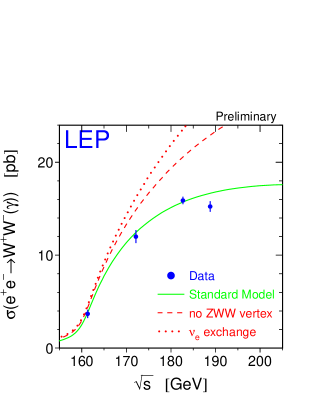
Figure 3: Measurements of $\sigma(e^{+}e^{-}\rightarrow W^{+}W^{-}$) [5].

We see in Fig. 4 that the $m_{W}$ measurements favour qualitatively $m_{H}<$ 300 GeV, though not at a high level of significance [5]. Stronger evidence for a light Higgs boson [26] is provided by the lower energy LEP 1, SLD and $\nu$N data, as also seen in Fig. 4. Combining all the precision electroweak data, one finds

$$m_{H}=76^{+85}_{-47}\pm 10~{}{\rm GeV}$$ (33)

as seen in Fig. 5, corresponding to $m_{H}<260$ GeV at the $95\%$ confidence level, if one uses a conservative error in $\alpha_{em}(m_{Z})$ and makes due allowance for unknown higher-loop uncertainties in the analysis [5].

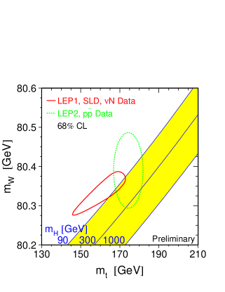
Figure 4: Contours of $m_{W}$ and $m_{t}$ from direct measurements (dotted ellipse) compared with predictions based on the precision electroweak data analyzed within the Standard Model (solid curve) [5]. Note the sensitivity to $m_{H}$.

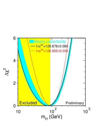
Figure 5: The $\chi^{2}$ function for a global fit to the precision electroweak data prefers $m_{H}\sim$ 100 GeV [5].

The range (33) may be compared with upper and lower bounds derived within the Standard Model. The tree-level unitarity limit $m_{H}\mathrel{\hbox to0.0pt{\raise 2.15277pt\hbox{$<$}\hss}{\lower 2.15277pt\hbox{$\sim$}}}$ 1 TeV [12, 13, 14] may be strengthened by including loop effects via renormalization-group calculations [27]. We see in Fig. 6 the upper bound on $m_{H}$ that is obtained by requiring the Standard Model  couplings to remain finite at all energies up to some cutoff $\Lambda:m_{H}\mathrel{\hbox to0.0pt{\raise 2.15277pt\hbox{$<$}\hss}{\lower 2.15277pt\hbox{$\sim$}}}$ 200 GeV if $\Lambda\simeq m_{P}$ and $m_{H}\mathrel{\hbox to0.0pt{\raise 2.15277pt\hbox{$<$}\hss}{\lower 2.15277pt\hbox{$\sim$}}}$ 700 GeV if $\Lambda\simeq m_{H}$, corresponding to upper limits from lattice calculations [28]. Also shown in Fig. 6 are lower limits on $m_{H}$ obtained by requiring that the effective Higgs potential remain positive for $|\phi|\mathrel{\hbox to0.0pt{\raise 2.15277pt\hbox{$<$}\hss}{\lower 2.15277pt\hbox{$\sim$}}}\Lambda:m_{H}\mathrel{\hbox to0.0pt{\raise 2.15277pt\hbox{$>$}\hss}{\lower 2.15277pt\hbox{$\sim$}}}$ 140 GeV if $\Lambda\simeq m_{P}$ [27].

Figure 6: The range of $m_{H}$ compatible with the Standard Model  remaining valid up to a high scale $\Lambda$ [27].

It is depressing to note that the range (33) of $m_{H}$ estimated on the basis of the precision electroweak data is compatible with the Standard Model remaining valid all the way up to the Planck scale: $\Lambda\simeq m_{P}$ . Moreover, the range (33) also imposes strong constraints on possible extensions of the Standard Model. For example, Fig. 7 shows that it effectively excludes a fourth generation [27]. Note that this renormalization-group argument is independent of the neutrino-counting argument (17) given earlier. In particular, this argument still holds if $m_{\nu_{4}}>m_{Z/2}$: in fact, it even becomes slightly stronger!

Figure 7: The regions of fourth-generation mass $m_{4}$ and Higgs mass $m_{H}$ compatible with the Standard Model remaining valid up to a high scale $\Lambda$ [27].

1.3 Defects of the Standard Model

It has been said repeatedly that there is no confirmed experimental evidence from accelerators against the Standard Model, and several possible extensions have been ruled out. Nevertheless, no thinking physicist could imagine that the Standard Model is the end of physics. Even if one accepts the rather bizarre set of group representations and hypercharges that it requires, the Standard Model  contains at least 19 parameters: 3 gauge couplings $g_{1,2,3}$ and 1 CP-violating non-perturbative vacuum angle $\theta_{3}$, 6 quark and 3 charged-lepton masses with 3 charged weak mixing angles and 1 CP-violating phase $\delta$, and 2 parameters: $(\mu,\lambda)$ or $(m_{H},m_{W})$ to characterize the Higgs sector. Moreover, many more parameters are required if one wishes to accommodate non-accelerator observations. For example, neutrino masses and mixing introduce at least 7 parameters: 3 masses, 3 mixing angles and 1 CP-violating phase, cosmological inflation introduces at least 1 new mass scale of order 10¹⁶ GeV, the cosmological baryon asymmetry is not explicable within the Standard Model, so one or more additional parameters are needed, and the cosmological constant may be non-zero. The ultimate “Theory of Everything” should explain all these as well as the parameters of the Standard Model.

It is convenient to organize the questions raised by the Standard Model into three broad categories. One is the Problem of Mass: do particle masses really originate from a Higgs boson, and, if so, why are these masses not much closer to the Planck mass $m_{P}\simeq 10^{19}$ GeV? This is the main subject of the next two lectures. Another is the Problem of Unification: can all the particle interactions be unified in a simple gauge group, and, if so, does it predict observable new phenomena such as baryon decay and/or neutrino masses, and does it predict relations between parameters of the Standard Model such as gauge couplings or fermion masses? This is the main subject of the fourth lecture. Then there is the Problem of Flavour: what is the origin of the six flavours each of quarks and leptons, and what explains their weak charged-current mixing and CP violation? This is the main subject of Yossi Nir’s lectures [29]. Finally, the quest for the Theory of Everything seems most promising in the context of string theory, particularly in its most recent incarnation of $M$ theory, as discussed in the fifth lecture, and by Michael Green [30]. In addition to all the above problems, this should also reconcile quantum mechanics with general relativity, explain the origin of space-time and the number of dimensions, make coffee, etc… .

2 INTRODUCTION TO SUPERSYMMETRY

2.1 The Electroweak Vacuum

We have discussed in Lecture 1 the fact that generating particle masses requires breaking the electroweak gauge symmetry spontaneously:

$$m_{W,Z}\not=0~{}\Leftrightarrow~{}~{}<0|X_{I,I_{3}}|0>~{}\not=0~{}$$ (34)

for some spin-0 quantity $X$ with non-zero isospin $I$ and third component $I_{3}$. The fact that experimentally $\rho\equiv m^{2}_{W}/m^{2}_{Z}~{}~{}\cos^{2}\theta_{W}\simeq 1$ is consistent with the Standard Model  expectation that $X$ has mainly $I={1\over 2}$ [4]. This is also what is required to give non-zero fermion masses: $m_{f}\bar{f}_{L}f_{R}+h.c.$, since the $f_{L,R}$ have $I={1\over 2},0$. The question then remains: what is the nature of $X$? In particular, is it elementary or composite?

The former is the option chosen in the Standard Model: $X=H:<0|H^{0}|0>\not=0$. However, as discussed in more detail later, quantum corrections to the squared mass of an elementary Higgs boson diverge quadratically:

$$\delta m^{2}_{H}=0\left({\alpha\over\pi}\right)\Lambda^{2}$$ (35)

where $\Lambda$ is some cutoff, corresponding physically to the scale up to which the Standard Model  remains valid. We discuss later the possibility that $\Lambda$ can be identified with the energy threshold for symmetry. This should occur at $\lambda\mathrel{\hbox to0.0pt{\raise 2.15277pt\hbox{$<$}\hss}{\lower 2.15277pt\hbox{$\sim$}}}$ 1 TeV, in order that the quantum corrections (35) have the same magnitude as the physical Higgs boson mass.

The alternative option is that $X$ is composite, namely a fermion-antifermion condensate $<0|\bar{F}F|0>\not=0$. This idea is motivated by the existence of a quark-antiquark condensate $<0|\bar{q}q|0>\not=0$ in QCD, and the rôle of Cooper pairs $<0|e^{-}e^{-}|0>\not=0$ in conventional superconductivity. Two major possibilities for the condensate have been considered: a top-antitop condensate $<0|\bar{t}t|0>\not=0$ held together by a large Yukawa coupling $\lambda_{H\bar{t}t}$ [31], and technicolour [32], in which new interactions that become strong at an energy scale $\Lambda\sim$ 1 TeV bind new strongly-interacting technifermions: $<0|\bar{T}T|0>\not=0$. The $\bar{t}t$ condensate idea is currently disfavoured, since simple implementations require $m_{t}>$ 200 GeV in contradiction with experiment, so we concentrate here on the technicolour alternative.

The technicolour idea [32] was initially modelled on the known dynamics of QCD:

$$<0|\bar{q}_{L}q_{R}+h.c.|0>\not=0\rightarrow<0|\bar{F}_{L}F_{R}+h.c.|0>\not=0$$ (36)

which breaks isospin with $I={1\over 2}$, if the electroweak multiplet assignments of the $F_{L}$ and $F_{R}$ are the same as those of the $q_{L}$ and $q_{R}$. The scale of this breaking will be appropriate if $\Lambda_{QCD}\rightarrow\Lambda_{TC}\sim$ 1 TeV. Just as QCD contains (if $m_{q}=0$) massless pions with the axial-current matrix element $<0|A_{\mu}|\pi>=ip_{\mu}f_{\pi}$, one expects a similar coupling

$$<0|J_{\mu}|\pi_{TC}>=ip_{\mu}F_{\pi}$$ (37)

for the technipion $\pi_{TC}$, which does the same Goldstone-eating job as (8), (9) if $F_{\pi}=v\simeq$ 250 GeV. If there are two massless flavours of technifermions, one expects 3 massless technipions to be eaten by the $W^{\pm}$ and $Z^{0}$, and the physical Higgs boson is replaced by an effective massive composite scalar, analogous to the scalar mesons of QCD and weighing 0(1) TeV. However, a single technidoublet is not enough when one imposes the necessary cancellation of anomalies and tries to give masses to conventional fermions [33]. For these reasons, the Standard Technicolour Model used to include a full technigeneration: $[(N,E),(U,D)_{1,2,3}]_{1,\ldots,N_{TC}}$, where the indices denote colour and technicolour indices. For generality, one can study models as functions of the numbers of techniflavours and technicolours: $(N_{TF},N_{TC})$.

Their effects via one-loop quantum corrections can be parametrized in terms of their contributions to electroweak observables via three combinations of vacuum polarizations [34, 35]. One example is:

$$T\equiv{\epsilon_{1}\over\alpha}\equiv{\Delta\rho\over\alpha}~{}:~{}\Delta\rho={\pi_{ZZ}(0)\over m^{2}_{Z}}-{\pi_{WW}(0)\over m^{2}_{W}}-2\tan\theta_{W}{\pi_{\gamma Z}(0)\over m^{2}_{Z}}$$ (38)

which describes deviations from the tree-level relation $\rho\equiv m^{2}_{W}/m^{2}_{Z}\cos^{2}\theta=1$ and measures isospin-breaking effects. This is related to $\Delta r$  (23) and receives contributions from Standard-Model particles:

$$T\ni{3\over 16\pi}~{}~{}{1\over\sin^{2}\theta_{W}\cos^{2}\theta_{W}}~{}~{}\left({m^{2}_{t}\over m^{2}_{W}}\right)-{3\over 16\pi\cos^{2}\theta_{W}}~{}~{}\ln\left({m^{2}_{H}\over m^{2}_{Z}}\right)+\ldots$$ (39)

The other relevant combinations of vacuum polarizations are [34, 35]

$$S\equiv{4\sin^{2}\theta_{W}\over\alpha}~{}~{}\epsilon_{3}\ni{1\over 12\pi}~{}~{}\ln\left({m^{2}_{H}\over m^{2}_{Z}}\right)+\ldots$$ (40)

and [34, 35]

$$U\equiv-{4\sin^{2}\theta_{W}\over\alpha}~{}~{}\epsilon_{2}$$ (41)

The precision electroweak data may be used to constrain $(S,T,U)$ (or $\epsilon_{1,2,3}$), and thereby possible extensions of the Standard Model with the same $SU(2)\times U(1)$ gauge group and additional matter particles, such as technicolour. Note, however, that this approach is not adequate for precision analyses of theories with important vertex diagrams such as the Standard Model  or its minimal supersymmetric extension, to be discussed later. These have important vertex and box diagrams, as well as the vacuum-polarization diagrams taken care of by $S,T,U(\epsilon_{1,2,3}$. Some of these be treated by introducing further parameters such as $\epsilon_{b}$ for the $Z\bar{b}b$ vertex. Even so, two-loop and other higher-order effects are not treated exactly in this approach.

Figure 8 compiles the constraints on $\sin^{2}\theta_{W}$ and the overall $Z$ weak coupling strength coming from the precision electroweak data (top panel) and the resulting constraints on $S$ and $T$ (bottom panel) [36]. We see that the lower-energy data are compatible with the high-energy data at around the one-$\sigma$ level, and that the high-energy data impose strong constraints on $S,T,U$ (equivalent to $\epsilon_{1,2,3}$). Figure 9 shows the available constraints in the $(\epsilon_{1},\epsilon_{2})$ plane [37]. We see that the one-loop corrections are certainly needed, since the data lie many $\sigma$ away from the (improved) Born approximation. We also see that the data are quite consistent with the Standard Model. A compilation of determinations of the $\epsilon_{i}$ are shown in Fig. 10 [37], where we see a discrepancy only in $\epsilon_{b}$, but even this is only slightly more than one $\sigma$. Finally, Fig. 11 compares the data constraint in the $(S,T)$ plane not only with the Standard Model but also with various technicolour models [36]. The models chosen all have one technidoublet, and hence $N_{TF}=2$, and varying values of $N_{TC}$ = 2,3,4. We see that even the least disfavoured model is at least four $\sigma$ away from the data, and models with larger $N_{TC}$ (shown) and $N_{TF}$ (not shown) deviate even further from experiment.

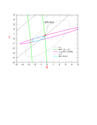
Figure 8: Constraints on $S$ and $T$ inferred from precision electroweak measurements at low and high energies [36].

Figure 9: Constraints on $(\epsilon_{1},\epsilon_{2})$ from precision electroweak measurements, which agree with the Standard Model predictions [37]. Note that the data lie many standard deviations away from the values expected (“Born”) if quantum corrections are neglected.

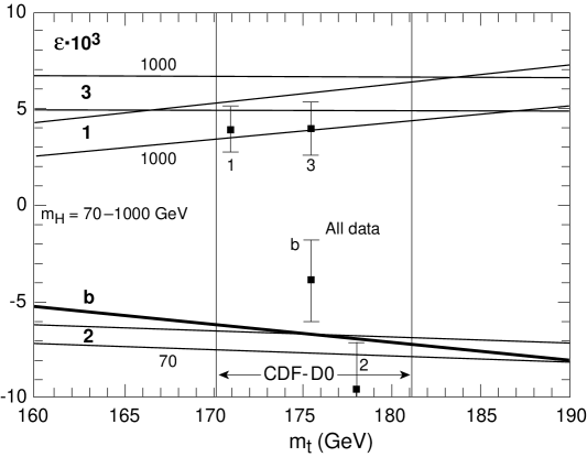
Figure 10: Values of the quantum corrections $\epsilon_{i}$ inferred from the data [37], compared with the Standard Model predictions.

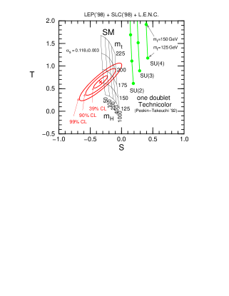
Figure 11: Values of $S$ and $T$ extracted from the data (ellipses) [36], confronted with the predictions of the Standard Model and of one-doublet technicolour models.

This large discrepancy has almost been the death of technicolour models, but various suggestions have been made that one could respect the experimental constraints if the technicolour dynamics is somewhat different from that of QCD. Specifically, it has been suggested that the technicolour coupling may not run as rapidly as the strong coupling [38]. Unfortunately, calculations in this framework of “walking technicolour” cannot be made as pecisely as in the conventional technicolour models discussed above, rendering it difficult to test or disprove. For the moment, no calculable technicolour model is consistent with the precision electroweak data, so we turn to supersymmetry.

2.2 Introduction to supersymmetry

Back in the 1960’s there were many (forgettable) attempts to combine internal symmetries such as flavour isospin or $SU(3)$ with relativistic external symmetries such as Lorentz invariance. However, in 1967 Coleman and Mandula [39] proved that this could not be done using only bosonic charges. The way to avoid this no-go theorem was found in 1971, when Gol’fand and Likhtman [40] showed that one could extend the Poincaré algebra using fermionic charges. In the same year, Neveu, Schwarz and Ramond [41] invented supersymmetry in two dimensions when they discovered how to incorporate fermions in string models. Supersymmetric field theories in four dimensions were discovered in 1973, by Volkov and Akulov [42] in a non-linear realization, and by Wess and Zumino [43] in the linear realization now used in most model-building. Soon afterwards, Wess, Zumino, Iliopoulos and Ferrara [44] realized that supersymmetric models were free of many of the divergences found in other four-dimensional field theories. Then, in 1976, Freedman, van Nieuwenhuizen and Ferrara [45] and independently Deser and Zumino [46] showed how supersymmetry can be realized locally (by analogy with gauge theories) in the context of supergravity.

Many of the ideas for using supersymmetry were motivated by the desire to unify known bosons and fermions: for example, unifying mesons and baryons motivated the early string work [41] and that of Wess and Zumino [43]. It was initially suggested that neutrino could be a Goldstone fermion in a non-linear realization of supersymmetry [42], but it was soon pointed out that experimental data on $\nu$ interaction cross sections conflicted with theorems on the low-energy behaviour in such theories [47]. The fact that supersymmetric theories had fewer (in some cases, no) divergences offered to some people who never liked infinite renormalizations hope that one could construct a finite theory. Others were attracted by the idea that supersymmetry might relate the odd-person-out Higgs boson to fermionic matter and perhaps gauge bosons. At a more fundamental level, the fact that local supersymmetry involves gravity suggested to many the idea of unifying all the particles and their interactions in some supergravity theory. However, this motivation did not provide a clear clue as to the mass scale of supersymmetry breaking, so there was no obvious reason why the sparticle masses should not be as heavy as $m_{P}\simeq 10^{19}$ GeV.

Such a reason was eventually provided by the mass hierarchy problem [48]: why is $m_{W}\ll m_{P}$? The latter is the only candidate we have for a fundamental mass scale in physics, where gravity is expected to become as strong as other particle interactions, e.g., graviton exchange at LEP 10¹⁹ would be comparable to $\gamma$ and $Z^{0}$ exchange. The hierarchy problem can be rephrased as: “why is $G_{F}\gg G_{N}$?”, since $G_{F}\sim 1/m^{2}_{W}$ and $G_{N}=1/m^{2}_{P}$. Alternatively, for the benefit of atomic, molecular and condensed-matter physicists, not to mention chemists and biologists, one can ask: why is the Coulomb potential in an atom so much larger than the Newton potential? The former is $e^{2}/r:e^{2}$ = 0(1), whereas the latter is $G_{N}m_{p}m_{e}/r$, so the Newton potential is negligible just because conventional particle masses $m_{p,e}$ are much lighter than $m_{P}$.

You might think that one could just set $m_{W}\ll m_{P}$ by hand, and ignore the problem. However, there is a threat from radiative corrections [48]. Each of the one-loop diagrams in Fig. 12 is individually quadratically divergent, implying

$$\delta m^{2}_{H,W}={\cal O}\left({g^{2}\over 16\pi^{2}}\right)~{}~{}\int^{\Lambda}d^{4}k{1\over k^{2}}={\cal O}\left({\alpha\over\pi}\right)\Lambda^{2}$$ (42)

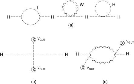
Figure 12: (a) One-loop quantum corrections to $m^{2}_{H}$ in the Standard Model. (b) Tree-level and (c) one-loop corrections to $m^{2}_{H}$ in a GUT.

where the cutoff $\Lambda$ in the integral represents the scale up to which the Standard Model  remains valid, and beyond which new physics sets in. If we think $\Lambda\simeq m_{P}$ or the grand unification scale, the quantum correction (42) is much larger than the physical value of $m_{H,W}\sim$ 100 GeV. This is not a problem for renormalization theory: there could be a large bare contribution with the opposite sign, and one could fine-tune its value to many significant figures so that the physical value $m^{2}_{H,W}\simeq\delta m^{2}_{H,W}$ (42). However, this seems unnatural, and would have to repeated order by order in perturbation theory. In contrast, the one-loop corrections to a fundamental fermion mass $m_{f}$ are proportional to $m_{f}$ itself, and only logarithmically divergent:

$$\delta m_{f}={\cal O}\left({g^{2}\over 16\pi^{2}}\right)m_{f}\int^{\Lambda}d^{4}k{1\over k^{4}}={\cal O}\left({\alpha\over\pi}\right)m_{f}\ln{\Lambda\over m_{f}}$$ (43)

This correction is no larger numerically than the physical value, for any $\Lambda\mathrel{\hbox to0.0pt{\raise 2.15277pt\hbox{$<$}\hss}{\lower 2.15277pt\hbox{$\sim$}}}m_{P}$. This is because there is a chiral symmetry reflected in the $m_{f}$ factor in (43) that keeps the quantum corrections naturally (logarithmically) small. The hope is to find a corresponding symmetry principle to make small boson masses natural: $\delta m^{2}_{H,W}\mathrel{\hbox to0.0pt{\raise 2.15277pt\hbox{$<$}\hss}{\lower 2.15277pt\hbox{$\sim$}}}m^{2}_{H,W}$.

This is achieved by supersymmetry [49], exploiting the fact that the boson and fermion loop diagrams in Fig. 12a have opposite signs. If there are equal numbers of fermions and bosons, and if they have equal couplings as in a supersymmetric theory, the quadratic divergences (42) cancel:

$$\delta m^{2}_{H,W}=-\left({g^{2}_{F}\over 16\pi^{2}}\right)~{}~{}(\Lambda^{2}+M^{2}_{F})+\left({g^{2}_{B}\over 16\pi^{2}}\right)~{}~{}(\Lambda^{2}+M^{2}_{B})={\cal O}\left({\alpha\over 4\pi}\right)~{}~{}|m^{2}_{B}-m^{2}_{f}|$$ (44)

This is no larger than the physical value: $\delta m^{2}_{H,W}\mathrel{\hbox to0.0pt{\raise 2.15277pt\hbox{$<$}\hss}{\lower 2.15277pt\hbox{$\sim$}}}m^{2}_{H,W}$, and hence naturally small, if

$$|m^{2}_{B}-m^{2}_{F}|\mathrel{\hbox to0.0pt{\raise 2.15277pt\hbox{$<$}\hss}{\lower 2.15277pt\hbox{$\sim$}}}1~{}{\rm TeV}^{2}$$ (45)

This naturalness argument [48] is the only available theoretical motivation for thinking that supersymmetry may manifest itself at an accessible energy scale.

However, this argument is qualitative, and a matter of taste. It does not tell us whether sparticles should appear at 900 GeV, 1 TeV or 2 TeV, and some theorists reject it altogether. They say that, in a renormalizable theory such as the Standard Model, one need not worry about the fine-tuning of a bare parameter, since it is not physical. However, I take naturalness seriously as a physical argument: it is telling us that a large hierarchy is intrinsically unstable, and supersymmetry is the most plausible way of stabilizing it. Moreover, many logarithmic divergences are absent in supersymmetry, which stabilizes the possible GUT Higgs corrections to $m_{H}$ shown in Fig. 12b arising from the loops shown in Fig. 12c, which is also important for stabilizing the hierarchy $m_{W}\ll m_{GUT}$, as we see later.

2.3 What is supersymmetry?

After all this introduction and motivation, just what is supersymmetry [49]? It is a symmetry that links bosons and fermions via spin-${1\over 2}$ charges $Q_{\alpha}$ (where $\alpha$ is a spinorial index). It seems to be the last possible symmetry of the particle scattering matrix [50]. As such, many would argue that it must inevitably play a rôle in physics, and it has in fact already appeared at a phenomenological level in condensed-matter, atomic and nuclear physics. All previously-known symmetries are generated by bosonic charges, which are, apart from the momentum operator $P_{\mu}$ associated with Lorentz invariance, scalar charges $Q$ that relate different particles of the same spin $J$: $Q|J>=|J^{\prime}>$, $Q\in U(1),SU(2),SU(3),\ldots$. Indeed, as already mentioned, Coleman and Mandula [39] showed that it was impossible to mix such internal symmetries with Lorentz invariance using bosonic charges. The essence of their proof is easy to grasp.

Consider $2\rightarrow 2$ scattering: $1+2\rightarrow 3+4$, and consider the possibility that there is a conserved tensor charge $\Sigma_{\mu\nu}$ corresponding to some higher bosonic symmetry (there can be no other charge with one vector index, besides $P_{\mu}$, and higher tensor charges can be discussed analogously to $\Sigma_{\mu\nu}$). Its diagonal matrix elements are required by Lorentz invariance to have the following tensor decomposition:

$$<a|\Sigma_{\mu\nu}|a>=\alpha p^{a}_{\mu}p^{a}_{\nu}+\beta g_{\mu\nu}$$ (46)

where $p^{a}_{\mu}$ is the four-momentum of the particle $a$ and $\alpha,\beta$ are unkown reduced matrix elements. For $\Sigma_{\mu\nu}$ to be conserved in the scattering process, as long as $\alpha\not=0$ one must require

$$p^{1}_{\mu}p^{1}_{\nu}+p^{2}_{\mu}p^{2}_{\nu}=p^{3}_{\mu}p^{3}_{\nu}+p^{4}_{\mu}p^{4}_{\nu}$$ (47)

as well as $p^{1}_{\mu}+p^{2}_{\mu}=p^{3}_{\mu}+p^{4}_{\mu}$. It is easy to convince oneself that the only possible simultaneous solutions to these linear and quadratic conservation conditions correspond to purely forward scattering. This conflicts [39] with the basic principles of quantum field theory as well as experiment.

This argument is fine as far as it goes, but it does not apply to any spinorial charge $Q_{\alpha}$, since the diagonal matrix elements vanish: $<a|Q_{\alpha}|a>=0$.

Let us explore now what is the possible algebra of an algebra of such spinorial charges $Q^{i}_{\alpha}:i=1,2,\ldots,N$ [50]. If they are to be symmetry generators, they must commute with the Hamiltonian:

$$[Q^{i}_{\alpha},H]=0$$ (48)

Hence, their anticommutator (which is bosonic) must also commute with $H$:

$$[\{Q^{i}_{\alpha},Q^{j}_{\beta}\},H]=0$$ (49)

By the Coleman-Mandula theorem [39], this anticommutator must be a combination of the conserved Lorentz vector charge $P_{\mu}$ and some scalar charge $Z^{ij}$. The only possible form is in fact

$$\{Q^{i}_{\alpha},Q^{j}_{\beta}\}=2\delta^{ij}(\gamma^{\mu}C)_{\alpha\beta}P_{\mu}+Z^{ij}$$ (50)

where we use four-component spinors, $C$ is the charge-conjugation matrix and $Z^{ij}$ is antisymmetric in the supersymmetry indices $\{i,j\}$. Thus, this so-called “central charge” vanishes for the $N=1$ case of phenomenological relevance.

The basic building blocks of $N=1$ supersymmetric theories are supermultiplets containing the following helicity states [49]:

$${\rm chiral}~{}:~{}~{}\left(\matrix{{1\over 2}\cr 0}\right)~{},~{}~{}{\rm gauge}~{}:~{}~{}\left(\matrix{1\cr{1\over 2}}\right)~{},~{}~{}{\rm graviton}~{}:~{}~{}\left(\matrix{2\cr{3\over 2}}\right)~{},$$ (51)

which are used to describe matter and Higgses, gauge fields and gravity, respectively. You may wonder why one does not use theories with extended supersymmetry: $N\geq 2$. The building blocks for $N=2$ are:

$${\rm matter}~{}:~{}~{}\left(\matrix{{1\over 2}\cr 0\cr-{1\over 2}}\right)~{},~{}~{}{\rm gauge}~{}:~{}~{}\left(\matrix{1\cr{1\over 2}\cr 0}\right)~{},~{}~{}{\rm gravity}~{}:~{}~{}\left(\matrix{2\cr{3\over 2}\cr 1}\right)~{},$$ (52)

and it is apparent that left- and right-handed particles (helicities $\mp$ 1/2) must be in identical representations of the gauge group. This is immediate for the matter supermultiplet in (52), and must also be the case for fermions in the gauge supermultiplet, since the helicity $\mp 1$ must be in identical adjoint representations. Hence an $N=2$ theory cannot accommodate parity violation, and is not suitable for phenomenology .

The simplest $N=1$ supersymmetric field theory contains a free fermion and a free boson [49, 52]:

$${\cal L}=\partial_{\mu}\phi^{*}~{}~{}\partial^{\mu}\phi+i~{}~{}\psi^{+}\bar{\sigma}\cdot\partial\psi$$ (53)

where we work with two-component spinors and denote $\sigma_{\mu}=(1,\underline{\sigma}),~{}~{}\bar{\sigma}_{\mu}=(1,-\underline{\sigma})$, where the $\underline{\sigma}$ are Pauli matrices. The simple supersymmetry transformation laws are

$$\delta_{\xi}\phi=\sqrt{2}\xi^{T}C\psi~{},~{}~{}\delta_{\xi}\psi=\sqrt{2}i\sigma\cdot\partial\phi C\xi^{*}$$ (54)

where $\xi$ is an infinitesimal spinor parameter and $C$ is the conjugation matrix: $C=-i\sigma^{2}=C^{*}$, $C^{-1}=C^{T}=-C$. It is easy to check that under (54) the Lagrangian (53) changes by a total derivative $\partial_{\mu}(\ldots)$, and hence the action $A=\int d^{4}x{\cal L}(x)$ is invariant. We can also see in (54) a reflection of the supersymmetry algebra (50): after two supersymmetry transformations, the fields $(\phi,\psi)$ are transformed by derivatives $(\partial\phi,\partial\psi)$, corresponding to the action of the momentum operator $P_{\mu}=i\partial_{\mu}$.

The example (54) can easily be extended to include interactions [49, 52]:

$${\cal L}=\partial_{\mu}\phi^{*}\partial^{\mu}\phi+i\psi^{\dagger}\bar{\sigma}\cdot\partial\psi+F^{\dagger}F+\left(F{\partial W\over\partial\phi}-{1\over 2}\psi^{T}C\psi{\partial^{2}W\over\partial\phi^{2}}+{\rm herm.conj.}\right)$$ (55)

with supersymmetry transformations:

$$\delta_{\xi}\phi=\sqrt{2}\xi^{T}C\psi~{},~{}~{}\delta_{\xi}\psi=\sqrt{2}i\sigma\cdot\partial\phi C\xi^{*}+\xi F~{},~{}~{}\delta_{\xi}F=-\sqrt{2}i\xi^{\dagger}\bar{\sigma}\cdot\partial\psi$$ (56)

The field $F$ is called an auxiliary field: notice that it has no kinetic term, and so may be eliminated by using an equation of motion:

$$F^{\dagger}=-{\partial W\over\partial\phi}$$ (57)

Thus all the matter interactions are characterized by the analytic function $W(\phi)$, which is called the superpotential. Renormalizability of the field theory requires the superpotential to be a cubic function: for $W=\lambda\phi_{1}\phi_{2}\phi_{3}$, one obtains from (55) the following particle interactions:

$$\lambda\left[(\psi^{T}_{1}C\psi_{2})\phi_{3}+(\psi^{T}_{2}C\psi_{3})\phi_{1}+(\psi^{T}_{3}C\psi_{1})\phi_{2}\right]+|\lambda\phi_{1}\phi_{2}|^{2}+|\lambda\phi_{2}\phi_{3}|^{2}+|\lambda\phi_{3}\phi_{1}|^{2}$$ (58)

where the last terms provide a quartic potential for the scalar fields $\phi_{i}$ and are called in the jargon “$F$ terms”.

We shall not discuss here in detail the construction of the interactions of a chiral supermultiplet with a gauge supermultiplet [49], limiting ourselves to quoting the results. In addition to the gauge interactions of the chiral fermions and their bosonic partners, there are gaugino interactions

$$\sqrt{2}g\left[(\psi^{T}_{i}C(T^{a})^{i}_{j}V_{a})\phi^{j*}+{\rm herm.conj.}\right]$$ (59)

where $(T^{a})^{i}_{j}$ is the gauge representation matrix for the chiral fields. There is also another quartic potential term for the scalars:

$$V={g^{2}\over 2}~{}\sum_{a}~{}~{}|\phi^{i^{*}}~{}(T^{a})^{j}_{i}~{}~{}\phi_{j}|^{2}$$ (60)

which are called in the jargon “$D$ terms”. Finally, we note for completeness that the conventional gauge-boson kinetic term and the gauge interactions of fermions in the adjoint representation of the gauge group, such as the gauginos $\tilde{V}_{a}$, are automatically supersymmetric.

2.4 Minimal Supersymmetric Extension of the Standard Model

Let us now return to phenomenology. If one is to construct a minimal supersymmetric model, the first natural question is: can one construct it out of the Standard Model particles alone? It is easy to see that this is impossible, because the known bosons and fermions have different conserved quantum numbers [53]. For example, gluons are in an octet (8) representation of colour, whereas quarks are in triplet (3) representation of colour. Similarly, there are no known weak-isotriplet fermions, as would be needed to partner the electroweak gauge bosons. The known leptons are isodoublets like the Higgs boson, but they carry lepton number, unlike the Higgs. For these reasons, new particles must be postulated [53] as supersymmetric partners of known particles, as seen in the Table.

Particle	Spin	Spartner	Spin
quark: $q$	${1\over 2}$	squak: $\tilde{q}$	0
lepton: $\ell$	${1\over 2}$	slepton: $\tilde{\ell}$	0
photon: $\gamma$	1	photino: $\tilde{\gamma}$	${1\over 2}$
$W$	1	wino: $\tilde{W}$	${1\over 2}$
$Z$	1	zino: $\tilde{Z}$	${1\over 2}$
Higgs: $H$	0	higgsino: $\tilde{H}$	${1\over 2}$

Table 1: Particles in the Standard Model and their supersymmetric partners.

The minimal supersymmetric extension of the Standard Model  (MSSM) [54] has the same gauge interactions as the Standard Model. In addition, there are couplings of the form (58) derived from the following superpotential:

$$W=\lambda_{d}~{}Q~{}D^{C}~{}H+\lambda_{\ell}~{}L~{}E^{C}~{}H+\lambda_{u}~{}Q~{}U^{C}~{}\bar{H}+\mu\bar{H}H$$ (61)

Here, $Q[L]$ denote isodoublets of supermultiplets containing $(u,d)_{L}[(\nu,\ell)_{L}],~{}D^{C}[U^{C},E^{C}]$ are singlets containing the left-handed conjugates $d^{C}_{L}[u^{C}_{L},e^{C}_{L}]$ of the right-handed $d_{R}[u_{R},e_{R}]$, and the superpotential couplings $\lambda_{d}[\lambda_{u,\ell}]$ correspond to the Yukawa couplings of the Standard Model  that give masses to the $d[u,\ell^{-}]$, respectively:

$$m_{d}=\lambda_{d}<H>~{},~{}~{}m_{u}=\lambda_{u}<\bar{H}>~{},~{}~{}m_{\ell}=\lambda_{\ell}<H>~{}.$$ (62)

Each of these should be understood as a $3\times 3$ matrix in generation space, which is to be diagonalized as in the Standard Model.

In addition to the Standard-Model-like superpotential interactions shown in (61), the following superpotential couplings [55] are also permitted by the gauge symmetries of the Standard Model:

$$W\ni\lambda LLE^{C}+\lambda^{\prime}QD^{C}L+\lambda^{\prime\prime}U^{C}D^{C}D^{C}$$ (63)

Each of these violate conservation of either lepton number $L$ or baryon number $B$. The possible presence of such interactions attracted some interest in 1997 [56, 57] with the discovery of unexpectedly many events at HERA at large $x$ and $Q^{2}$ [58], but interest has now subsided. Their potential significance is only discussed intermittently in these lectures.

Note that (61) requires two Higgs doublets $H,\bar{H}$ with opposite hypercharges in order to give masses to all the matter fermions. In the Standard Model, one doublet $\phi$ and its complex conjugate $\phi^{\dagger}$ would have sufficed. This does not work in the MSSM, because the superpotential $W$ must be an analytic function of the fields. Moreover, Higgs supermultiplets include Higgsino fermions that generate triangle anomalies which must cancel among themselves, requiring at least two Higgs doublets. These couple via the $\mu$ term in (61). Note also that the ratio of Higgs vacuum expectation values

$$\tan\beta\equiv{<\bar{H}>\over<H>}$$ (64)

is undetermined and should be treated as a free parameter. Finally, we comment that the superpotential and gauge couplings determine the MSSM’s quartic scalar couplings, providing important constraints on the Higgs masses, as we see later.

Before discussing in more detail the phenomenology of the MSSM, it is appropriate to mention two important but indirect experimental indications that favour supersymmetry. One is the relatively light mass of the Higgs boson inferred from the analysis of precision electroweak data [5], as seen in Fig. 5. As discussed in more detail in the next Lecture, the lightest MSSM Higgs boson must weigh $\mathrel{\hbox to0.0pt{\raise 2.15277pt\hbox{$<$}\hss}{\lower 2.15277pt\hbox{$\sim$}}}$ 150 GeV [59], in good agreement with the range favoured by the data. The other indication in favour of supersymmetry is the measured value of $\sin^{2}\theta_{W}$ [5], as shown in Fig. 2. As discussed in more detail in Lecture 4, Grand Unified Theories predict $\sin^{2}\theta_{W}$ as a function of $\alpha_{s}(m_{Z})$. For the measured value of $\alpha_{s}(m_{Z})$, GUTs without supersymmetry predict $\sin^{2}\theta_{W}\sim$ 0.21 to 0.22 [7], whereas GUTs with supersymmetry at the TeV scale predict $\sin^{2}\theta_{W}\sim$ 0.23 [9], in much better agreement with the data [60].

These two experimental arguments buttress the theoretical argument given earlier, which was based on the hierarchy problem. Put together, these provide ample motivation for studying the phenomenology of the MSSM in more detail, as we do in the next Lecture.

3 PHENOMENOLOGY OF SUPERSYMMETRY

3.1 Soft Supersymmetry Breaking

The first issue that must be addressed in the phenomenology of supersymmetry is the sad fact that no sparticles have ever been detected. This means that sparticles do not weigh the same as their supersymmetric partners: $m_{\tilde{e}}\not=m_{e},~{}~{}m_{\tilde{\gamma}}\not=m_{\gamma}$, etc., and hence that supersymmetry must be broken. We return in Lecture 5 to review some theoretical ideas about the origin of supersymmetry breaking, restricting ourselves here to a phenomenological parametrization [61]. Any such parametrization should retain the desirable features of supersymmetry, particularly the absence of power-law divergences. This “softness” requirement means that any supersymmetry-breaking interactions ${\cal L}_{\rm susyX}$ should have quantum field dimension $<4$ (recall that the quantum field dimension of a boson (derivative) (fermion) is $1(1)({3\over 2}$)), and hence a positive power of some numerical mass parameters, so that $\int d^{4}x{\cal L}_{\rm susyX}$ is dimensionless. There are in fact further restrictions on soft supersymmetry-breaking parameters [62], and a general parametrization comprises scalar mass terms: $m^{2}_{0_{i}}|\phi_{i}|^{2}$, gaugino masses: ${1\over 2}M_{a}~{}\tilde{V}^{T}_{a}~{}C\tilde{V}_{a}$, and trilinear or bilinear scalar interactions proportional to superpotential terms: $A_{\lambda}\lambda\phi^{3}$, $B_{\mu}\mu\phi^{2}$. Note some absences from this list, including masses for fermions in chiral supermultiplets $m_{\psi}\psi^{T}C\psi$ and non-analytic trilinear scalar couplings $\propto\phi^{*}\phi^{2}$.

We shall adopt for now the hypothesis (to be discussed in Lecture 5) that the soft supersymmetry-breaking masses $m^{2}_{0_{i}},M_{a},A_{\lambda},B_{\mu}$ originate at some high GUT or gravity scale, perhaps from some supergravity or superstring mechanism. The physical values of the soft supersymmetry-breaking parameters are then subject to logarithmic renormalizations that may be calculated and resummed using the renormalization-group techniques familiar from QCD [63], which also figure in the GUT calculations of $\sin^{2}\theta_{W}$ that are reviewed in Lecture 4. Renormalizations by gauge interactions have the general structure

$$m^{2}_{0_{i}}\rightarrow m^{2}_{0_{i}}+C^{a}_{i}M^{2}_{a}~{},~{}~{}M_{a}\rightarrow{\alpha_{a}\over\alpha_{GUT}}~{}M_{a}$$ (65)

at the one-loop level, and higher-loop renormalizations are also well understood [64].

It is often assumed that the soft supersymmetry-breaking masses are universal at the GUT or supergravity scale:

$$m^{2}_{0_{i}}\equiv m^{2}_{0}~{},~{}~{}M_{a}\equiv m_{1/2}~{},~{}~{}A_{\lambda}\equiv A~{},~{}~{}B_{\mu}\equiv B$$ (66)

but this hypothesis is not very well motivated, since, in particular, general supergravity models give no theoretical hint why they should be universal. Some superstring models give hints of universality for the gaugino masses $m_{1/2}$, but universality for the scalar masses $m^{2}_{0_{i}}$ is more questionable. Since a high degree of universality is suggested (at least for the first two generations) by flavour-changing neutral-current (FCNC) constraints [65], this provides some impetus for models guaranteeing scalar-mass universality, such as the gauge-mediated or messenger models [66] discussed briefly in Lecture 5. If one assumes universality, the parameters $\mu,\tan\beta,m_{0},m_{1/2},A$ suffice to characterize MSSM phenomenology.

Figure 13 shows the results of some typical renormalization-group calculations assuming universal inputs [67]. We see that scalar masses are generally renormalized to larger values as the scale is reduced, but this is not necessarily the case if there are large Yukawa interactions such as those of the top quark, which may modify (65) in the case of Higgs masses. Such Yukawa effects involving the top quark must certainly be taken into account, and could also be important for the bottom quark and the $\tau$ lepton if $\tan\beta$ is large. The potential significance of these Yukawa interactions is that they tend to drive $m^{2}_{H}$ to smaller values at smaller renormalization scales $\mu$ [68]

$$\mu{d\over{\rm ln}\mu}m_{h}^{2}={1\over(4\pi)^{2}}\left(3\lambda_{t}^{2}(m_{h}^{2}+m_{\tilde{q}}^{2}+m_{t}^{2})+\dots\right)$$ (67)

where $m_{\tilde{q}}$ is a squark mass.

Figure 13: Renormalization-group evolution of soft supersymmetry-breaking mass parameters [67].

This makes it possible to generate electroweak symmetry breaking dynamically, even if $m^{2}_{H}>0$ at the input scale along with the other scalar mass-squared parameters [68], as seen in Fig. 13. The appropriate renormalization scale for discussing the effective Higgs potential of the MSSM is $Q\mathrel{\hbox to0.0pt{\raise 2.15277pt\hbox{$<$}\hss}{\lower 2.15277pt\hbox{$\sim$}}}$ 1 TeV, and the electroweak gauge symmetry will be broken if either or both of $m^{2}_{H_{1,2}}(Q)<0$, as in the model potential (5). This is certainly possible for $m_{t}\sim$ 175 GeV as observed.

3.2 Supersymmetric Higgs Bosons

As was discussed in Lecture 2, one expects two complex Higgs doublets $H_{2}\equiv(H^{+}_{2},H^{0}_{2})~{},~{}~{}H_{1}\equiv(H^{+}_{1},H^{0}_{1})$ in the MSSM, with a total of 8 real degrees of freedom. Of these, 3 are eaten via the Higgs mechanism to become the longitudinal polarization states of the $W^{\pm}$ and $Z^{0}$, leaving 5 physical Higgs bosons to be discovered by experiment. Three of these are neutral: the lighter CP-even neutral $h$, the heavier CP-even neutral $H$, the CP-odd neutral $A$, and charged bosons $H^{\pm}$. The quartic potential is completely determined by the $D$ terms (59)

$$V_{4}={g^{2}+g^{\prime 2}\over 8}~{}~{}\left(|H^{0}_{1}|^{2}-|H^{0}_{2}|^{2}\right)$$ (68)

for the neutral components, whilst the quadratic terms may be parametrized at the tree level by

$${1\over 2}=m^{2}_{H_{1}}~{}|H_{1}|^{2}+m^{2}_{H_{2}}~{}|H_{2}|^{2}+(m^{2}_{3}~{}H_{1}H_{2}+{\rm herm.conj.})$$ (69)

where $m^{2}_{3}=B_{\mu}\mu$. One combination of the three parameters $(m^{2}_{H_{1}},m^{2}_{H_{2}},m^{2}_{3})$ is fixed by the Higgs vacuum expectation $v=\sqrt{v^{2}_{1}+v^{2}_{2}}$ = 246 GeV, and the other two combinations may be rephrased as $(m_{A},\tan\beta)$. These characterize all Higgs masses and couplings in the MSSM at the tree level. Looking back at (18), we see that the gauge coupling strength of the quartic interactions (68) suggests a relatively low mass for at least the lightest MSSM Higgs boson $h$, and this is indeed the case, with $m_{h}\leq m_{Z}$ at the tree level:

$$m^{2}_{h}=m^{2}_{Z}~{}\cos^{2}2\beta$$ (70)

This raised considerable hope that the lightest MSSM Higgs boson could be discovered at LEP, with its prospective reach to $m_{H}\sim$ 100 GeV.

However, radiative corrections to the Higgs masses are calculable in a supersymmetric model (this was, in some sense, the whole point of introducing supersymmetry!), and they turn out to be non-negligible for $m_{t}\sim$ 175 GeV [59]. Indeed, the leading one-loop corrections to $m^{2}_{h}$ depend quartically on $m_{t}$:

$$\Delta m^{2}_{h}={3m^{4}_{t}\over 4\pi^{2}v^{2}}~{}~{}\ln~{}~{}\left({m_{\tilde{t}_{1}}m_{\tilde{t}_{2}}\over m^{2}_{t}}\right)+{3m^{4}_{t}\hat{A}^{2}_{t}\over 8\pi^{2}v^{2}}~{}~{}\left[2h(m^{2}_{\tilde{t}_{1}},m^{2}_{\tilde{t}_{2}})+\hat{A}^{2}_{t}~{}~{}f(m^{2}_{\tilde{t}_{1}},m^{2}_{\tilde{t}_{2}})\right]+\ldots$$ (71)

where $m_{\tilde{t}_{1,2}}$ are the physical masses of the two stop squarks $\tilde{t}_{1,2}$ to be discussed in more detail shortly, $\hat{A}_{t}\equiv A_{t}-\mu\cot\beta$, and

$$h(a,b)\equiv{1\over a-b}~{}\ln\left({a\over b}\right)~{},~{}~{}f(a,b)={1\over(a-b)^{2}}~{}\left[2-{a+b\over a-b}~{}\ln\left({a\over b}\right)\right]$$ (72)

Non-leading one-loop corrections to the MSSM Higgs masses are also known, as are corrections to coupling vertices, two-loop corrections and renormalization-group resummations [69]. For $m_{\tilde{t}_{1m2}}\mathrel{\hbox to0.0pt{\raise 2.15277pt\hbox{$<$}\hss}{\lower 2.15277pt\hbox{$\sim$}}}$ 1 TeV and a plausible range of $A_{t}$, one finds

$$m_{h}\mathrel{\hbox to0.0pt{\raise 2.15277pt\hbox{$<$}\hss}{\lower 2.15277pt\hbox{$\sim$}}}130~{}{\rm GeV}$$ (73)

as seen in Fig. 14. There we see the sensitivity of $m_{h}$ to $(m_{A},\tan\beta)$, and we also see how $m_{A},m_{H}$ and $m_{H^{\pm}}$ approach each other for large $m_{A}$.

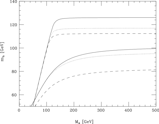
Figure 14: The lightest Higgs boson mass in the MSSM, for different values of $\tan\beta$ and the CP-odd Higgs boson mass $M_{A}$ [25].

The radiative corrections (71), (72) have major implications for experiments and accelerators. They may push the MSSM Higgs sector beyond the reach of LEP 2 and into the lap of the LHC [70]. They motivate the optimization of LHC detectors for the Higgs mass range (73). They may motivate the orientation of future $e^{+}e^{-}$ linear-collider construction so as to study such an MSSM Higgs boson in more detail than is possible at the LHC [71].

The decay modes of the MSSM Higgs bosons have been carefully studied, as seen in Fig. 15 [71]. Like the single Higgs boson of the Standard Model, the lightest MSSM Higgs boson $h$ prefers to decay into the heaviest particles available, typically $h\rightarrow\bar{b}b$, and this has been the primary focus of searches at LEP 2. However, there are “blind spots” in MSSM parameter space where this decay mode is suppressed by cancellations, complicating the search at LEP 2. Ignoring this possible complication, Fig. 16 shows the regions of MSSM parameter that may be explored at LEP 2 for different centre-of-mass energies and luminosities. After LEP 2, the Fermilab Tevatron collider has a chance of observing $h\rightarrow\bar{b}b$ and possibly other decays [72], if it accumulates sufficient luminosity. The potential for LHC searches for MSSM Higgs bosons is shown in Fig. 17 for one choice of the MSSM parameters [70]. We see that the entire parameter space is covered at maximum luninosity, though with considerable reliance on the rare decay mode $h\rightarrow\gamma\gamma$.

Figure 15: The expected decay modes of the lightest MSSM Higgs boson $h$ [71].

Figure 16: Prospective discovery and exclusion limits for MSSM Higgs searches at LEP.

Figure 17: Prospective coverage of the MSSM Higgs sector at the LHC [70].

3.3 Sparticle Masses and Mixing

We now progress to a more complete discussion of sparticle masses and mixing.

Sfermions : Each flavour of charged lepton or quark has both left- and right-handed components $f_{L,R}$, and these have separate spin-0 boson superpartners $\tilde{f}_{L,R}$. These have different isospins $I={1\over 2},~{}0$, but may mix as soon as the electroweak gauge symmetry is broken. Thus, for each flavour we should consider a $2\times 2$ mixing matrix for the $\tilde{f}_{L,R}$, which takes the following general form [73]:

$$M^{2}_{\tilde{f}}\equiv\left(\matrix{m^{2}_{\tilde{f}_{LL}}&m^{2}_{\tilde{f}_{LR}}\cr\cr m^{2}_{\tilde{f}_{LR}}&m^{2}_{\tilde{f}_{RR}}}\right)$$ (74)

The diagonal terms may be written in the form

$$m^{2}_{\tilde{f}_{LL,RR}}=m^{2}_{\tilde{f}_{L,R}}+m^{D^{2}}_{\tilde{f}_{L,R}}+m^{2}_{f}$$ (75)

where $m_{f}$ is the mass of the corresponding fermion, $\tilde{m}^{2}_{\tilde{f}_{L,R}}$ is the soft supersymmetry-breaking mass discussed in the previous section, and $m^{D^{2}}_{\tilde{f}_{L,R}}$ is a contribution due to the quartic $D$ terms in the effective potential:

$$m^{D^{2}}_{\tilde{f}_{L,R}}=m^{2}_{Z}~{}\cos 2\beta~{}~{}(I_{3}+\sin^{2}\theta_{W}Q_{em})$$ (76)

where the term $\propto I_{3}$ is non-zero only for the $\tilde{f}_{L}$. Finally, the off-diagonal mixing term takes the general form

$$m^{2}_{\tilde{f}_{L,R}}=m_{f}\left(A_{f}+\mu^{\tan\beta}_{\cot\beta}\right)~{}~{}{\rm for}~{}~{}f=^{e,\mu,\tau,d,s,b}_{u,c,t}$$ (77)

It is clear that $\tilde{f}_{L,R}$ mixing is likely to be important for the $\tilde{t}$, and it may also be important for the $\tilde{b}_{L,R}$ and $\tilde{\tau}_{L,R}$ if $\tan\beta$ is large. We also see from (75) that the diagonal entries for the $\tilde{t}_{L,R}$ would be different from those of the $\tilde{u}_{L,R}$ and $\tilde{c}_{L,R}$, even if their soft supersymmetry-breaking masses were universal, because of the $m^{2}_{f}$ contribution. In fact, we also expect non-universal renormalization of $m^{2}_{\tilde{t}_{LL,RR}}$ (and also $m^{2}_{\tilde{b}_{LL,RR}}$ and $m^{2}_{\tilde{\tau}_{LL,RR}}$ if $\tan\beta$ is large), because of Yukawa effects analogous to those discussed in the previous section for the renormalization of the soft Higgs masses.

For these reasons, the $\tilde{t}_{L,R}$ are not usually assumed to be degenerate with the other squark flavours. Indeed, one of the $\tilde{t}$ could well be the lightest squark, perhaps even lighter than the $t$ quark itself [73]. The mass limits [16] combined in Fig. 18 assume degenerate $(\tilde{u},\tilde{d},\tilde{s},\tilde{c},\tilde{b})_{L,R}$, even though this degeneracy should also be broken by the flavour-universal $D$ terms (76) and by renormalization effects that are different for $\tilde{f}_{L,R}$. The search for the stop mass eigenstates $\tilde{t}_{1,2}$ requires a separate analysis. Figure 19 shows the experimental lower limits on $m_{\tilde{t}_{1}}$ from ALEPH and $D\phi$ for different assumed values of the $\tilde{t}$ mixing angle $\theta_{\tilde{t}}$ [16], and assuming that $\tilde{t}\rightarrow c\chi$ decay dominates, where $\chi$ is the lightest neutralino.

Figure 18: Excluded domains in the search for light stops and neutralinos, as a function of the stop mixing angle $\theta_{\tilde{t}}$ [16].

Figure 19: Excluded regions in gluino and squark masses [16].

Charginos: These are the supersymmetric partners of the $W^{\pm}$ and $H^{\pm}$, which mix through a $2\times 2$ matrix

$$-{1\over 2}~{}(\tilde{W}^{-},\tilde{H}^{-})~{}~{}M_{C}~{}~{}\left(\matrix{\tilde{W}^{+}\cr\tilde{H}^{+}}\right)~{}~{}+~{}~{}{\rm herm.conj.}$$ (78)

where

$$M_{C}\equiv\left(\matrix{M_{2}&\sqrt{2}m_{W}\sin\beta\cr\sqrt{2}m_{W}\cos\beta&\mu}\right)$$ (79)

Here $M_{2}$ is the unmixed $SU(2)$ gaugino mass and $\mu$ is the Higgs mixing parameter introduced in (61). Figure 20 displays (among other lines to be discussed later) the contour $m_{\chi^{\pm}}$ = 91 GeV for the lighter of the two chargino mass eigenstates [74]. Some recent experimental lower limits on $m_{\chi^{\pm}}$ as functions of the other MSSM parameters are shown in Fig. 21 [16].

Figure 20: The $(\mu,M_{2})$ plane characterizing charginos and neutralinos, for (a) $\mu<0$ and (b) $\mu>0$, including contours of $m_{\chi}$ and $m_{\chi^{\pm}}$, and of neutralino purity [74].

Figure 21: Lower limits on the chargino mass inferred in the higgsino region (top panels) and the gaugino region (bottom panels) [16].

Neutralinos: These are characterized by a $4\times 4$ mass mixing matrix [75], which takes the following form in the $(\tilde{W}^{3},\tilde{B},\tilde{H}^{0}_{2},\tilde{H}^{0}_{1})$ basis :

$$m_{N}=\left(\matrix{M_{2}&0&{-g_{2}v_{2}\over\sqrt{2}}&{g_{2}v_{1}\over\sqrt{2}}\cr\cr 0&M_{1}&{g^{\prime}v_{2}\over\sqrt{2}}&{-g^{\prime}v_{1}\over\sqrt{2}}\cr\cr{-g_{2}v_{2}\over\sqrt{2}}&{g^{\prime}v_{2}\over\sqrt{2}}&0&\mu\cr\cr{g_{2}v_{1}\over\sqrt{2}}&{-g^{\prime}v_{1}\over\sqrt{2}}&\mu&0}\right)$$ (80)

Note that this has a structure similar to $M_{C}$ (79), but with its entries replaced by $2\times 2$ submatrices. As has already been mentioned, one conventionally assumes that the $SU(2)$ and $U(1)$ gaugino masses $M_{1,2}$ are universal at the GUT or supergravity scale, so that

$$M_{1}\simeq M_{2}~{}~{}{\alpha_{1}\over\alpha_{2}}$$ (81)

so the relevant parameters of (80) are generally taken to be $M_{2}=(\alpha_{2}/\alpha_{GUT})m_{1/2}$, $\mu$ and $\tan\beta$.

Figure 20 also displays contours of the mass of the lightest neutralino $\chi$, as well as contours of its gaugino and Higgsino contents [74]. In the limit $M_{2}\rightarrow 0$, $\chi$ would be approximately a photino and it would be approximately a Higgsino in the limit $\mu\rightarrow 0$. Unfortunately, these idealized limits are excluded by unsuccessful LEP and other searches for neutralinos and charginos, as we now discuss in more detail.

3.4 The Lightest Supersymmetric Particle

This is expected to be stable in the MSSM, and hence should be present in the Universe today as a cosmological relic from the Big Bang [76, 75]. Its stability arises because there is a multiplicatively-conserved quantum number called $R$ parity, that takes the values +1 for all conventional particles and -1 for all sparticles [53]. The conservation of $R$ parity can be related to that of baryon number $B$ and lepton number $L$, since

$$R=(-1)^{3B+L+2S}$$ (82)

where $S$ is the spin. Note that $R$ parity could be violated either spontaneously if $<0|\tilde{\nu}|0>\not=0$ or explicitly if one of the supplementary couplings (63) is present. There could also be a coupling $HL$, but this can be defined away be choosing a field basis such that $\bar{H}$ is defined as the superfield with a bilinear coupling to $H$. Note that $R$ parity is not violated by the simplest models for neutrino masses, which have $\Delta L=0,\pm 2$, nor by the simple GUTs discussed in the next Lecture, which violate combinations of $B$ and $L$ that leave $R$ invariant. There are three important consequences of $R$ conservation:

1. sparticles are always produced in pairs, e.g., $\bar{p}p\rightarrow\tilde{q}\tilde{g}X$, $e^{+}e^{-}\rightarrow\tilde{\mu}+\tilde{\mu}^{-}$,

2. heavier sparticles decay to lighter ones, e.g., $\tilde{q}\rightarrow q\tilde{g},\tilde{\mu}\rightarrow\mu\tilde{\gamma}$, and

3. the lightest sparticles is stable,

because it has no legal decay mode.

This feature constrains strongly the possible nature of the lightest supersymmetric sparticle. If it had either electric charge or strong interactions, it would surely have dissipated its energy and condensed into galactic disks along with conventional matter. There it would surely have bound electromagnetically or via the strong interactions to conventional nuclei, forming anomalous heavy isotopes that should have been detected. There are upper limits on the possible abundances of such bound relics, as compared to conventional nucleons [77]:

$${n({\rm relic})\over n(p)}\mathrel{\hbox to0.0pt{\raise 2.15277pt\hbox{$<$}\hss}{\lower 2.15277pt\hbox{$\sim$}}}10^{-15}~{}~{}{\rm to}~{}~{}10^{-29}$$ (83)

for 1 GeV $\mathrel{\hbox to0.0pt{\raise 2.15277pt\hbox{$<$}\hss}{\lower 2.15277pt\hbox{$\sim$}}}m_{\rm relic}\mathrel{\hbox to0.0pt{\raise 2.15277pt\hbox{$<$}\hss}{\lower 2.15277pt\hbox{$\sim$}}}$ 1 TeV. These are far below the calculated abundances of such stable relics:

$${n({\rm relic})\over n(p)}\mathrel{\hbox to0.0pt{\raise 2.15277pt\hbox{$>$}\hss}{\lower 2.15277pt\hbox{$\sim$}}}10^{-6}~{}~{}(10^{-10})$$ (84)

for relic particles with electromagnetic (strong) interactions. We may conclude [75] that any supersymmetric relic is probably electromagnetically neutral with only weak interactions, and could in particular not be a gluino. Whether the lightest hadron containing a gluino is charged or neutral, it would surely bind to some nuclei. Even if one pleads for some level of fractionation, it is difficult to see how such gluino nuclei could avoid the stringent bounds established for anomalous isotopes of many species [77].

Plausible scandidates of different spins are the sneutrinos $\tilde{\nu}$ of spin 0, the lightest neutralino $\chi$ of spin 1/2, and the gravitino $\tilde{G}$ of spin 3/2. The sneutrinos have been ruled out by the combination of LEP experiments and direct searches for cosmological relics. Neutrino counting (17) requires $m_{\tilde{\nu}}\mathrel{\hbox to0.0pt{\raise 2.15277pt\hbox{$>$}\hss}{\lower 2.15277pt\hbox{$\sim$}}}$ 43 GeV [78], in which case the direct relic searches in underground low-background experiments require $m_{\tilde{\nu}}\mathrel{\hbox to0.0pt{\raise 2.15277pt\hbox{$>$}\hss}{\lower 2.15277pt\hbox{$\sim$}}}$ 1 TeV [79]. The gravitino cannot be ruled out, and its popularity has revived somewhat with the renaissance of gauge-mediated (messenger) models [66], as described in Lecture 5. For the rest of this Lecture, however, we condentrate on the neutralino possibility.

A very attractive feature of the neutralino candidature for the lightest supersymmetric particle is that it has a relic density of interest to astrophysicists and cosmologists: $\Omega_{\chi}h^{2}={\cal O}(0.1)$ over generic domains of the MSSM parameter space [75]. This feature is seen clearly in Fig. 22, where $0.1<\Omega_{\chi}h^{2}<0.3$ is possible in a large area of the $(\mu,M_{2})$ plane for suitable choices of the other MSSM parameters [74]. In this domain, the lightest neutralino $\chi$ could constitute the cold dark matter favoured by theories of cosmological structure formation [80].

Figure 22: Contours of $\Omega h^{2},m_{h},m_{\chi^{\pm}}$ and higgsino purity in the $(\mu,M_{2})$ plane, for (a) $\mu<0$ and (b) $\mu>0$ [74].

We have already seen in Fig. 21 some of the experimental limits on chargino and neutralino production, that may be used to set interesting limits on $m_{\chi}$. One example is shown in Fig. 23, where one particular choice of $m_{0}$ is assumed [16]. (This parameter is relevant because $\tilde{\nu}$ exchange contributes to $\sigma(e^{+}e^{-}\rightarrow\chi^{+}\chi^{-})$, and the $\tilde{\nu}$ and $\tilde{e}$ masses influence $\chi^{\pm}$ decay patterns [78].) It is interesting to note in Fig. 23 that LEP 1 data (e.g., neutrino counting in $Z^{0}$ decays (17)) did not by themselves provide an absolute lower limit on $m_{\chi}$: this became possible only by combining them with higher-energy LEP data [78].

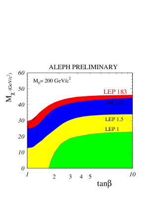
Figure 23: Experimental lower limit on the lightest neutralino mass, as a function of $\tan\beta$, assuming $m_{0}$ = 200 GeV [16].

The lower limit on $m_{\chi}$ can be strengthened by combining the direct chargino/neutralino searches with other experimental and theoretical constraints [78, 74], as illustrated in Fig. 24. The dotted lines labelled LEP are the analogues of Fig. 23, but with $m_{0}$ allowed to float freely. The dotted lines marked $H,C$ incorporate the experimental lower limit on $m_{h}$ and the cosmological relic-density constraint $\Omega_{\chi}h^{2}\leq$ 0.3, respectively. The solid lines marked $UHM$ further assume universal scalar masses for the Higgs multiplets. The lines marked cosmo, $DM$ combine this assumption with the relic-density assumptions $\Omega_{\chi}h^{2}<$ 0.3, $>$0.1, respectively. Figure 24 documents a lower limit $m_{\chi}>$ 40 GeV [81], which can be strengthened using more recent LEP 2 data to about 45 GeV [74]. We expect that higher-energy runs of LEP will extend this sensitivity to $m_{\chi}\sim$ 50 GeV. We also see in Fig. 24 that this type of combined analysis of the MSSM parameter space imposes an absolute lower limit on $\tan\beta$. Data from LEP that have been published so far indicate that $\tan\beta\mathrel{\hbox to0.0pt{\raise 2.15277pt\hbox{$>$}\hss}{\lower 2.15277pt\hbox{$\sim$}}}$ 1.8 [74], and future LEP runs will be sensitive up to $\tan\beta\sim 3$, principally via Higgs searches.

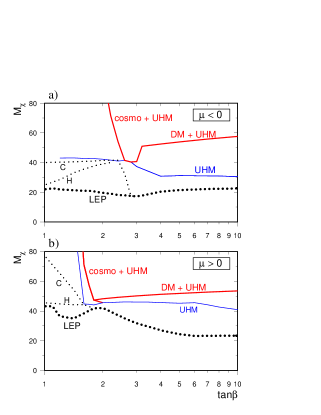
Figure 24: Lower limits on $m_{\chi}$ from LEP (thick dots), Higgs searches (H), cosmological limits on $\Omega h^{2}$ (c), which are strengthened by assuming universal scalar masses for Higgs bosons (UHM), also in combination with the constraints $\Omega h^{2}<0.3$ (cosmo + UHM) and $\Omega h^{2}>0.1$ (DM + UHM) [78].

We close with a few comments on the prospects for sparticle searches at the LHC. These should be able to extend the squark and gluino searches up to masses on 2.5 GeV, as seen in Fig. 25 [82]. By looking in several different channels: missing energy $E^{miss}_{T}$ with 0, 1, 2, etc. leptons, it should be possible to explore several times over the domain of parameter space of interest to cosmologists where $\Omega_{\chi}h^{2}\mathrel{\hbox to0.0pt{\raise 2.15277pt\hbox{$<$}\hss}{\lower 2.15277pt\hbox{$\sim$}}}0.4$, as also seen in Fig. 25 . Moreover, it should be possible to reconstruct several different sparticles via the cascade decays of squarks and gluinos, and even make detailed mass measurements that could test supergravity mass relations [84].

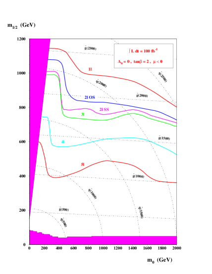
Figure 25: Regions of the $(m_{0},m_{1/2})$ plane that can be explored at the LHC [82].

3.5 The “Anomaly” that Went Away$\ldots$

For some time, measurements of $R_{b}=\Gamma(Z^{0}\rightarrow\bar{b}b)/\Gamma(Z\rightarrow$ all hadrons) seemed to be in significant disagreement with the Standard Model, generating considerable interest. It was suggested that the discrepancy might be explicable by one-loop supersymmetric radiative corrections, due either to Higgs exchange if $m_{A}$ were small and $\tan\beta$ large, or to chargino and stop exchange if both $m_{\chi^{\pm}}$ and $m_{\tilde{t}}$ were small, as well as $\tan\beta$ [85]. The Higgs former scenario was early effectively excluded by early Higgs searches at LEP, but the $\chi^{\pm}/\tilde{t}$ scenario fitted well with theoretical prejudices and survived somewhat longer. It was particularly interesting, because it suggested that either a chargino or a stop might be light enough to be produced at LEP 2 or at the Fermilab Tevatron collider.

As time has progressed, the $R_{b}$ anomaly has steadily decreased in significance, and is now barely a one-$\sigma$ discrepancy, as seen in Fig. 26 [5]. In parallel, both LEP 2 and the Tevatron have explored considerable domains of MSSM parameter space, excluding significant domains of $m_{\chi^{\pm}}$ and $m_{\tilde{t}}$. Might there still be a significant supersymmetric contribution to $R_{b}$, comparable to the experimental error $\Delta R_{b}\sim$ 0.0010 ? Even before the latest exclusion domains from LEP et al., we [86] found that, of about 500,000 possible choices of the basic MSSM model parameters, only 210 of those that respected the experimental constraints in early 1997 (including $b\rightarrow s\gamma$ and the cosmological relic density) could yield $\Delta R_{b}\geq$ 0.0010. This already made the case for a significant supersymmetric contribution to $R_{b}$ appear somewhat implausible. (Though everybody would have been happy if one of these “unusual” models was close to reality!) Another possible strike against these models was that they required a departure from the universality assumptions favoured in supergravity models, as seen in Fig. 27, where the “globular cluster” of “interesting” models with $\Delta R_{b}>$ 0.0010 is outside the zone of parameter space accessible in such universal supergravity models, which can only yield [86]

$$\Delta R_{b}<0.0003$$ (85)

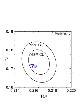
Figure 26: Experimental constraints on $Z\rightarrow\bar{b}b$ and $\bar{c}c$ decays compared with the Standard Model prediction [5].

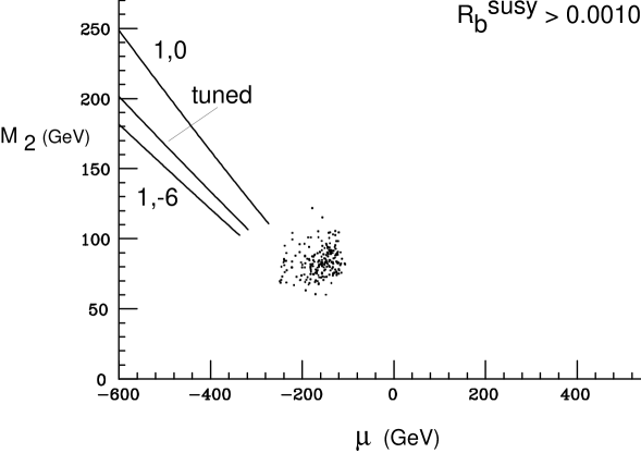
Figure 27: Region of the $(\mu,M_{2})$ plane where MSSM contributions to $R_{b}$ larger than 0.0010 are possible which cannot be attained in models with universal scalar masses (solid lines) [86].

Moreover, the “interesting” models all had $m_{\tilde{t}_{1}}<$ 100 GeV, and 90% of them have now been excluded by the more sensitive LEP 2 searches shown in Fig. 19. The conclusion must be that plausible parameter choices for the MSSM do not yield a significant contribution to $R_{b}$, and hence that it is legitimate to use the measurements in a global fit to the precision electroweak data in the Standard Model, as was assumed in Lecture 1.

4 GRAND UNIFICATION

4.1 Basic Strategy

The philosophy of grand unification [8, 87] is to seek a simple gauge group that includes the untidy $SU(3)$, $SU(2)$ and $U(1)$ gauge groups of QCD and the electroweak sector of the Standard Model. The hope is that this grand unification can be achieved while neglecting gravity, at least as a first approximation. If the grand unification scale turns out to be significantly less than the Planck mass, this is not obviously a false hope. We discuss later in this Lecture and the next the extent to which this hope is indeed realistic: for the moment we just note that the grand unification scale is indeed expected to be exponentially large:

$${m_{GUT}\over m_{W}}=\exp\left({\cal O}\left({1\over\alpha_{em}}\right)\right)$$ (86)

and typical estimates will be that $m_{GUT}=0(10^{16}$ GeV). Such a calculation involves an extrapolation of known physics by many orders of magnitude further than, e.g., the extrapolation that Newton made from the apple to the Solar System. However, it is not excluded by our current knowledge of the Standard Model. For example, we see in Fig. 6 that the estimate (33) of the Higgs mass is consistent with the Standard Model remaining valid all the way to the Planck scale $m_{P}\simeq 10^{19}$ GeV, and even far beyond.

If the grand unification scale is indeed so large, most tests of it are likely to be indirect, and we meet some later, such as relations between Standard Model gauge couplings and between particle masses. Any new interactions, such as those that might cause protons to decay or give masses to neutrinos, are likely to be very strongly suppressed.

The first apparent obstacle to the philosophy of grand unification is the fact that the strong coupling $\alpha_{3}=g^{2}_{3}/4\pi$ is indeed much stronger than the electroweak couplings at present-day energies: $\alpha_{3}\gg\alpha_{2},\alpha_{1}$. However, you have seen here in the lectures by Michelangelo Mangano [88] that the strong coupling is asymptotically free:

$$\alpha_{3}(Q)\simeq{12\pi\over(33-2N_{q})\ln(Q^{2}/\Lambda^{2}_{3})}+\ldots$$ (87)

where $N_{q}$ is the number of quarks, $\Lambda_{3}\simeq$ few hundred MeV is an intrinsic scale of the strong interactions, and the dots in (87) represent higher-loop corrections to the leading one-loop behaviour shown. The other Standard Model  gauge couplings also exhibit logarithmic violations analogous to (87). For example, the effective value of $\alpha_{em}(m_{Z})\sim 1/128$, with estimated ranges displayed in Fig. 5. The renormalization-group evolution for the $SU(2)$ gauge coupling is

$$\alpha_{2}(Q)\simeq{12\pi\over(22-2N_{q}-N_{H/2})\ln(Q^{2}/\Lambda^{2}_{2})}+\ldots$$ (88)

where we have assumed equal numbers of quarks and leptons, and $N_{H}$ is the number of Higgs doublets. Taking the inverses of (87) and (88), and then taking their difference, we find

$${1\over\alpha_{3}(Q)}-{1\over\alpha_{2}(Q)}=\left({11+N_{H/2}\over 12\pi}\right)\ln\left({Q^{2}\over m^{2}_{X}}\right)+\ldots$$ (89)

We have absorbed the scales $\Lambda_{3}$ and $\Lambda_{2}$ into a single grand unification scale $M_{X}$ where $\alpha_{3}=\alpha_{2}$.

Evaluating (89) when $Q={\cal O}(M_{W})$, where $\alpha_{3}\gg\alpha_{2}=0(\alpha_{em})$, we derive the characteristic feature (86) that the grand unification scale is exponentially large. As we see in more detail later, in most GUTs there are new interactions mediated by bosons weighing ${\cal O}(m_{X})$ that cause protons to decay with a lifetime $\alpha m^{4}_{X}$. In order for the proton lifetime to exceed the experimental limit, we need $m_{X}\mathrel{\hbox to0.0pt{\raise 2.15277pt\hbox{$>$}\hss}{\lower 2.15277pt\hbox{$\sim$}}}10^{14}$ GeV and hence $\alpha_{em}\mathrel{\hbox to0.0pt{\raise 2.15277pt\hbox{$<$}\hss}{\lower 2.15277pt\hbox{$\sim$}}}1/120$ in (86) [89]. On the other hand, if the neglect of gravity is to be consistent, we need $m_{X}\mathrel{\hbox to0.0pt{\raise 2.15277pt\hbox{$<$}\hss}{\lower 2.15277pt\hbox{$\sim$}}}10^{19}$ GeV and hence $\alpha_{em}\mathrel{\hbox to0.0pt{\raise 2.15277pt\hbox{$>$}\hss}{\lower 2.15277pt\hbox{$\sim$}}}1/170$ in (86) [89]. The fact that the measured value of the fine-structure constant $\alpha_{em}\simeq 1/137.03599959(38)13)$ lies in this allowed range may be another hint favouring the GUT philosophy.

Further empirical evidence for grand unification is provided by the previously-advertized prediction it makes for the neutral electroweak mixing angle [7]. Calculating the renormalization of the electroweak couplings, one finds:

$$\sin^{2}\theta_{W}={\alpha_{em}(m_{W})\over\alpha_{2}(m_{W})}\simeq{3\over 8}~{}~{}\left[1-{\alpha_{em}\over 4\pi}~{}~{}{110\over 9}\ln{m^{2}_{X}\over m^{2}_{W}}\right]$$ (90)

which can be evaluated to yield $\sin^{2}\theta_{W}\sim$ 0.210 to 0.220, if there are only Standard Model particles with masses $\mathrel{\hbox to0.0pt{\raise 2.15277pt\hbox{$<$}\hss}{\lower 2.15277pt\hbox{$\sim$}}}m_{X}$ [7]. This is to be compared with the experimental value $\sin^{2}\theta_{W}=0.23155\pm 0.00019$ shown in Fig. 2. Considering that $\sin^{2}\theta_{W}$ could a priori have had any value between 0 and 1, this is an impressive qualitative success. The small discrepancy can be removed by adding some extra particles, such as the supersymmetric particles in the MSSM.

Another qualitative success is the prediction of the $b$ quark mass [90, 91]. In many GUTs, such as the minimal $SU(5)$ model discussed shortly, the $b$ quark and the $\tau$ lepton have equal Yukawa couplings when renormalized at the GUT sale. The renormalization group then tells us that

$${m_{b}\over m_{\tau}}\simeq\left[\ln\left({m^{2}_{b}\over m^{2}_{X}}\right)\right]^{12\over 33-2N_{q}}$$ (91)

Using $m_{\tau}=$ 1.78 GeV, we predict that $m_{b}\simeq$ 5 GeV, in agreement with experiment. Happily, this prediction remains successful if the effects of supersymmetric particles are included in the renormalization-group calculations [92].

To examine the GUT predictions for $\sin^{2}\theta_{W}$, etc. in more detail, one needs to study the renormalization-group equations beyond the leading one-loop order. Through two loops, one finds that

$$Q~{}~{}{\partial\alpha_{i}(Q)\over\partial Q}=-{1\over 2\pi}~{}~{}\left(b_{i}+{b_{ij}\over 4\pi}~{}~{}\alpha_{j}(Q)\right)~{}~{}\left[\alpha_{i}(Q)\right]^{2}$$ (92)

where the $b_{i}$ receive the one-loop contributions

$$b_{i}=\left(\matrix{0\cr-{22\over 3}\cr-11}\right)+N_{g}\left(\matrix{{4\over 3}\cr\cr{4\over 3}\cr\cr{4\over 3}}\right)+N_{H}\left(\matrix{{1\over 10}\cr\cr{1\over 6}\cr\cr 0}\right)$$ (93)

from gauge bosons, $N_{g}$ matter generations and $N_{H}$ Higgs doublets, respectively, and at two loops

$$b_{ij}=\left(\matrix{0&0&0\cr\cr 0&-{136\over 3}&0\cr\cr 0&0&-102}\right)+N_{g}\left(\matrix{{19\over 15}&{3\over 5}&{44\over 15}\cr\cr{1\over 5}&{49\over 3}&4\cr\cr{4\over 30}&{3\over 2}&{76\over 3}}\right)+N_{H}\left(\matrix{{9\over 50}&{9\over 10}&0\cr\cr{3\over 10}&{13\over 6}&0\cr\cr 0&0&0}\right)$$ (94)

These coefficients are all independent of any specific GUT model, depending only on the light particles contributing to the renormalization. Including supersymmetric particles as in the MSSM, one finds [9]

$$b_{i}=\left(\matrix{0\cr\cr-6\cr\cr-9}\right)+N_{g}\left(\matrix{2\cr\cr 2\cr\cr 2}\right)+N_{H}\left(\matrix{{3\over 10}\cr\cr{1\over 2}\cr\cr 0}\right)$$ (95)

and

$$b_{ij}=\left(\matrix{0&0&0\cr\cr 0&-24&0\cr\cr 0&0&-54}\right)+N_{g}\left(\matrix{{38\over 15}&{6\over 5}&{88\over 15}\cr\cr{2\over 5}&14&8\cr\cr{11\over 5}&3&{68\over 3}}\right)+N_{H}\left(\matrix{{9\over 50}&{9\over 10}&0\cr\cr{3\over 10}&{7\over 2}&0\cr\cr 0&0&0}\right)$$ (96)

again independent of any specific supersymmetric GUT.

One can use these two-loop equations to make detailed calculations of $\sin^{2}\theta_{W}$ in different GUTs. These confirm that non-supersymmetric models are not consistent with the determinations of the gauge couplings from LEP and elsewhere [60]. Previously, we argued that these models predicted a wrong value for $\sin^{2}\theta_{W}$, given the experimental value of $\alpha_{3}$. In Fig. 28a we see the converse, namely that extrapolating the experimental determinations of the $\alpha_{i}$ using the non-supersymmetric renormalization-group equations (93), (94) does not lead to a common value at any renormalization scale. In contrast, we see in Fig. 28b that extrapolation using the supersymmetric renormalization-group equations (95), (96) does lead to possible unification at $m_{GUT}\sim 10^{16}$ GeV [93].

Figure 28: The measurements of the gauge coupling strengths at LEP (a) do not evolve to a unified value if there is no supersymmetry but do (b) if supersymmetry is included [93].

Turning this success around, and assuming $\alpha_{3}=\alpha_{2}=\alpha_{1}$ at $m_{GUT}$ with no threshold corrections at this scale, one may estimate that [94]

$$\sin^{2}\theta_{W}(M_{Z})\bigg{|}_{\overline{\rm MS}} = 0.2029+{7\alpha_{em}\over 15\alpha_{3}}+{\alpha_{em}\over 20\pi}\left[-3\ln\left({m_{t}\over m_{Z}}\right)+{28\over 3}\ln\left({m_{\tilde{g}}\over m_{Z}}\right)\right.$$ (97)

$$\left.-{32\over 3}\ln\left({m_{\tilde{W}}\over m_{Z}}\right)-\ln\left({m_{A}\over m_{Z}}\right)-4\ln\left({\mu\over m_{Z}}\right)+\ldots\right]$$

Setting all the sparticle masses to 1 TeV reproduces approximately the value of $\sin^{2}\theta_{W}$ observed experimentally. Can one invert this successful argument to estimate the supersymmetric particle mass scale? One can show [95] that the sparticle mass thresholds in (97) can be lumped into the parameter

$$T_{susy}\equiv|\mu|\left({m^{2}_{W}\over m_{\tilde{g}}}\right)^{14/19}~{}~{}\left({m^{2}_{A}\over\mu^{2}}\right)^{3/38}~{}~{}\left({m^{2}_{\tilde{W}}\over\mu^{2}}\right)^{2/19}~{}~{}\prod^{3}_{i=1}~{}~{}\left({m^{3}_{\tilde{\ell}_{Li}}m^{7}_{\tilde{q}_{i}}\over m^{2}_{\tilde{\ell}_{R_{i}}}m^{5}_{\tilde{u}_{i}}m^{3}_{\tilde{d}_{i}}}\right)^{1/19}$$ (98)

If one assumes sparticle mass universality at the GUT scale, then [95]

$$T_{susy}\simeq|\mu|\left({\alpha_{2}\over\alpha_{3}}\right)^{3/2}\simeq{\mu\over 7}$$ (99)

approximately. The measured value of $\sin^{2}\theta_{W}$ is consistent with $T_{susy}\sim$ 100 GeV to 1 TeV, roughly as expected from the hierarchy argument. However, the uncertainties are such that one cannot use this consistency to constrain $T_{susy}$ very tightly [96]. In particular, even if one accepts the universality hypothesis, there could be important model-dependent threshold corrections around the GUT scale [94, 97]. We are at the limit of what one can say without studying specific models, so let us now do so.

4.2 GUT Models

Before embarking on their study, however, we first clarify some necessary technical points. As well as looking for a simple unifying group $G\supset SU(3)\times SU(2)\times U(1)$, we shall be looking for unifying representations $R$ that contain both quarks and leptons. Since gauge interactions conserve helicity, any particles with the same helicity are fair game to appear in any GUT representation $R$, and it is convenient to work with states of just one helicity, say left-handed. The left-handed particle content of the Standard Model  is as follows. In each generation, there is a quark doublet $(u,d)_{L}$ which transforms as (3,2) of $SU(3)\times SU(2)_{L}$. Instead of working with the right-handed singlets $u_{R},d_{R}$ that have (3,1) representations, it is convenient to work with their antiparticles, which are left-handed: the $u^{c}_{L}$ and $d^{c}_{L}$ transform as $(\bar{3},1)$ of $SU(3)\times SU(2)_{L}$. Similarly each generation contains a lepton doublet $(\nu,\ell^{-})_{L}$ transforming as (1,2), and the right-handed charged lepton $\ell_{R}$ is replaced by its conjugate $\ell^{C}_{L}$, which transforms as a (1,1) of $SU(3)\times SU(2)_{L}$. We should also keep track of the hypercharges $Y=Q-I_{3}$. One of the major puzzles of the Standard Model  is why

$$\sum_{q,\ell}Q_{i}=3Q_{u}+3Q_{d}+Q_{e}=0$$ (100)

In the Standard Model, the hypercharge assignments are a priori independent of the $SU(3)\times SU(2)_{L}$ assignments, although constrained by the fact that quantum consistency requires the resulting triangle anomalies to cancel. In a simple GUT, the relation (100) is automatic: whenever $Q$ is a generator of a simple gauge group, $\sum_{R}Q=0$ for particles in any representation $R$ (consider, e.g., the values of $I_{3}$ in any representation of $SU(2)$).

The basic rules of GUT model-building are that one must look for (a) a gauge group of rank 4 or more – to accommodate the Standard Model  $SU(3)\times SU(2)\times U(1)$ gauge group – which (b) admits complex representations – to accommodate the known matter fermions. The rank of a gauge group is the number of generators that can be diagonalized simultaneously, i.e., the number of quantum numbers that it admits. For example, $SU(2)$ and $U(1)_{em}$ both have rank 1 corresponding to $I_{3}$ and $Q_{em}$, respectively, and $SU(3)$ has rank 2 corresponding to $T_{3}$ and $Y$. Complex representations are required to allow the violation of charge conjugation $C$, as required by the Standard Model, which has

$$(\nu,e)_{L}\in(1,2)~{},~{}~{}(u,d)_{L}\in(3,2)~{},~{}~{}e^{c}_{L}\in(1,1)~{},~{}~{}u^{c}_{L}~{},~{}~{}d^{c}_{L}\in(\bar{3},1)$$ (101)

as discussed above.

The following is the mathematical catalogue [8] of rank-4 gauge groups which are either simple or the direct products of identical simple gauge groups:

$$Sp(8)~{},~{}~{}SO(8)~{},~{}~{}SO(9)~{},~{}~{}F_{4}~{},~{}~{}SU(3)\times SU(3)~{},~{}~{}SU(5)$$ (102)

Among these, only $SU(3)\times SU(3)$ and $SU(5)$ have complex representations. Moreover, if one tried to use $SU(3)\times SU(3)$, one would need to embed the electroweak gauge group in the second $SU(3)$ factor. This would be possible only if $\sum_{q}Q_{q}=0=\sum_{\ell}Q_{\ell}$, which is not the case for the known quarks and leptons. Therefore, attention has focussed on $SU(5)$ [8] as the only possible rank-4 GUT group.

The useful representations of $SU(5)$ are the complex vector 5 representation denoted by $F_{\alpha}$, its conjugate $\underline{\bar{5}}$ denoted by $\bar{F}^{\alpha}$, the complex two-index antisymmetric tensor 10 representation $T_{[\alpha\beta]}$, and the adjoint 24 representation $A^{\alpha}_{\beta}$. The latter is used to accommodate the gauge bosons of $SU(5)$:

$$\left(\matrix{&&&\vdots&\bar{X}\;\;\bar{Y}\cr&g_{1,\ldots,8}&&\vdots&\bar{X}\;\;\bar{Y}\cr&&&\vdots&\bar{X}\;\;\bar{Y}\cr\dotfill\cr X&X&X&\vdots&\cr&&&\vdots&W_{1,2,3}\cr Y&Y&Y&\vdots&}\right)$$ (103)

where the $g_{1,\ldots,8}$ are the gluons of $SU(3)$, the $W_{1,2,3}$ are the $SU(2)$ weak bosons, the $U(1)$ hypercharge boson is proportional to the traceless diagonal generator $(1,1,1,-3/2,-3/2)$, and the $(X,Y)$ are (3,2) of new gauge bosons that we discuss in the next section.

The quarks and leptons of each generation are accommodated in $\underline{\bar{5}}$ and $\underline{10}$ representations of $SU(5)$:

$$\bar{F}=\left(\matrix{d^{c}_{R}\cr\cr d^{c}_{Y}\cr\cr d^{c}_{B}\cr\dotfill\cr-e^{-}\cr\nu_{e}}\right)_{L}~{},~{}~{}~{}T=\left(\matrix{0&u^{c}_{B}&-u^{c}_{Y}&\vdots&-u_{R}&-d_{R}\cr-u^{c}_{B}&0&u^{c}_{R}&\vdots&-u_{Y}&-d_{Y}\cr u^{c}_{Y}&-u^{c}_{R}&0&\vdots&-u_{B}&-d_{B}\cr\dotfill\cr u_{R}&u_{Y}&u_{B}&\vdots&0&-e^{c}\cr d_{R}&d_{Y}&d_{B}&\vdots&e^{c}&0}\right)_{L}$$ (104)

The particle assignments are unique up to the effects of mixing between generations, which we do not discuss in detail here [98]. The uniqueness is because

$$\underline{\bar{5}}=(\bar{3},1)+(1,2)~{},~{}~{}\underline{10}=(3,2)+(\bar{3},1)+(1,2)$$ (105)

in terms of $SU(3)\times SU(2)$ representations. Therefore, the $(\nu,e)_{L}$ doublet in (101) can only be assigned to the $\underline{\bar{5}}$, and since $\Sigma Q_{em}=0$ in any GUT representation, the $(\bar{3},1)$ in the $\underline{\bar{5}}$ must be assigned to the $d^{c}$ in (101). The remaining $(u,d)_{L}\in(3,2),u^{c}\in(\bar{3},1)$ and $e^{c}\in(1,1)$ in (101) fit elegantly into the 10, as seen in (104) and (105) .

The remaining steps in constructing an $SU(5)$ GUT are the choices of representations for Higgs bosons, first to break $SU(5)\rightarrow SU(3)\times SU(2)\times U(1)$ and subsequently to break the electroweak $SU(2)\times U(1)_{Y}\rightarrow U(1)_{em}$. The simplest choice for the first stage is an adjoint 24 of Higgs bosons $\Phi$:

$$<0|\Phi|0>=\left(\matrix{1&0&0&\vdots&0&0\cr 0&1&0&\vdots&0&0\cr 0&0&1&\vdots&0&0\cr\dotfill\cr 0&0&0&\vdots&-{3\over 2}&0\cr 0&0&0&\vdots&0&-{3\over 2}}\right)\times{\cal O}(m_{GUT})$$ (106)

It is easy to see that this v.e.v. preserves colour $SU(3)$ acting on the first three rows and columns, weak $SU(2)$ acting on the last two rows and columns, and the hypercharge $U(1)$ along the diagonal. The subsequent breaking of $SU(2)\times U(1)_{Y}\rightarrow U(1)_{em}$ is most economically accomplished by a 5 representation of Higgs bosons $H$:

$$<0|\phi|0>=(0,0,0,0,1)\times 0(m_{W})$$ (107)

It is clear that this has an $SU(4)$ symmetry which yields [90] the relation $m_{b}=m_{\tau}$ that leads, after renormalization (91), to a successful prediction for $m_{b}$ in terms of $m_{\tau}$. However, the same trick does not work for the first two generations, indicating a need for epicycles in this simplest GUT model [100].

Making the minimal $SU(5)$ GUT supersymmetric, as motivated by the naturalness of the gauge hierarchy, is not difficult [61]. One must replace the above GUT multiplets by supermultiplets: $\underline{\bar{5}}\bar{F}$ and 10 $T$ for the matter particles, 24 $\Phi$ for the GUT Higgs fields that break $SU(5)\rightarrow SU(3)\times SU(2)\times U(1)$. The only complication is that one needs 5 and $\underline{\bar{5}}$ Higgs representations $H$ and $\bar{H}$ to break $SU(2)\times U(1)_{Y}\rightarrow U(1)_{em}$, just as two doublets were needed in the MSSM. The Higgs potential is specified by the appropriate choice of superpotential [61]:

$$W=(\mu+{3\lambda\over 2}M)+\lambda\bar{H}\Phi H+f(\Phi)$$ (108)

where $f(\Phi)$ is chosen so that $\partial f/\partial\Phi=0$ when

$$<0|\Phi|0>=M\left(\matrix{1&0&0&\vdots&0&0\cr 0&1&0&\vdots&0&0\cr 0&0&1&\vdots&0&0\cr\dotfill\cr 0&0&0&\vdots&-{3\over 2}&0\cr 0&0&0&\vdots&0&-{3\over 2}}\right)$$ (109)

Inserting this into the second term of (108), one finds terms $\lambda M\bar{H}_{3}H_{3},~{}~{}-3/2\lambda M\bar{H}_{2}H_{2}$ for the colour-triplet and weak-doublet components of $\bar{H}$ and $H$, respectively. Combined with the bizarre coefficient of the first term, these lead to

$$W\ni(\mu+{5\lambda\over 2}M)\bar{H}_{3}H_{3}+\mu\bar{H}_{2}H_{2}$$ (110)

Thus we have heavy Higgs triplets (as needed for baryon stability, see the next section) and light Higgs doublets. This requires fine tuning the coefficient of the first term in $W$ (108) to about 1 part in $10^{13}$! The advantage of supersymmetry is that its no-renormalization theorems [44] guarantee that this fine tuning is “natural”, in the sense that quantum corrections like those in Fig. 12c do not destroy it, unlike the situation without supersymmetry. On the other hand, supersymmetry alone does not explain the origin of the hierarchy.

4.3 Baryon Decay

Baryon instability is to be expected on general grounds, since there is no exact gauge symmetry to guarantee that baryon number $B$ is conserved. Indeed, baryon decay is a generic prediction of GUTs, which we illustrate with the simplest $SU(5)$ model, that is anyway embedded in larger and more complicated GUTs. We see in (103) that there are two species of gauge bosons in $SU(5)$ that couple the colour $SU(3)$ indices (1,2,3) to the electroweak $SU(2)$ indices (4,5), called $X$ and $Y$. As we can see from the matter representations (104), these may enable two quarks or a quark and lepton to annihilate, as seen in Fig. 29a. Combining these possibilities leads to interactions with $\Delta B=\Delta L=1$. The forms of effective four-fermion interactions mediated by the exchanges of massive $Z$ and $Y$ bosons, respectively, are [91]:

$$\left(\epsilon_{ijk}u_{R_{k}}\gamma_{\mu}u_{L_{j}}\right)~{}~{}{g^{2}_{X}\over 8m^{2}_{X}}~{}~{}\left(2e_{R}~{}\gamma^{\mu}~{}d_{L_{i}}+e_{L}~{}\gamma^{\mu}~{}d_{R_{i}}\right)~{},$$

$$\left(\epsilon_{ijk}u_{R_{k}}\gamma_{\mu}d_{L_{j}}\right)~{}~{}{g^{2}_{Y}\over 8m^{2}_{X}}~{}~{}\left(\nu_{L}~{}\gamma^{\mu}~{}d_{R_{i}}\right)~{}.$$ (111)

up to generation mixing factors.

Figure 29: Diagrams contributing to baryon decay (a) in minimal $SU(5)$ and (b) in minimal supersymmetric $SU(5)$.

Since the gauge couplings $g_{X}=g_{Y}=g_{3,2,1}$ in an $SU(5)$ GUT, and $m_{X}\simeq m_{Y}$, we expect that

$$G_{X}\equiv{g^{2}_{X}\over 8m^{2}_{X}}\simeq G_{Y}\equiv{g^{2}_{Y}\over 8m^{2}_{Y}}$$ (112)

It is clear from (111) that the baryon decay amplitude $A\propto G_{X}$, and hence the baryon $B\rightarrow\ell+$ meson decay rate

$$\Gamma_{B}=cG^{2}_{X}m^{5}_{p}$$ (113)

where the factor of $m^{5}_{p}$ comes from dimensional analysis, and $c$ is a coefficient that depends on the GUT model and the non-perturbative properties of the baryon and meson.

The decay rate (113) corresponds to a proton lifetime

$$\tau_{p}={1\over c}~{}{m^{4}_{X}\over m^{5}_{p}}$$ (114)

It is clear from (114) that the proton lifetime is very sensitive to $m_{X}$, which must therefore be calculated very precisely. In minimal $SU(5)$, the best estimate was [101]

$$m_{X}\simeq(1~{}{\rm to}~{}2)\times 10^{15}\times\Lambda_{QCD}$$ (115)

where $\Lambda_{QCD}$ is the characteristic QCD scale in the $\overline{\rm MS}$ prescription with four active flavours. Making an analysis of the generation mixing factors [98], one finds that the preferred proton (and bound neutron) decay modes in minimal $SU(5)$ are

$$p\rightarrow e^{+}\pi^{0}~{},~{}~{}e^{+}\omega~{},~{}~{}\bar{\nu}\pi^{+}~{},~{}~{}\mu^{+}K^{0}~{},~{}~{}\ldots$$

$$n\rightarrow e^{+}\pi^{-}~{},~{}~{}e^{+}\rho^{-}~{},~{}~{}\bar{\nu}\pi^{0}~{},~{}~{}\ldots$$ (116)

and the best numerical estimate of the lifetime is [101]

$$\tau(p\rightarrow e^{+}\pi^{0})\simeq 2\times 10^{31\pm 1}\times\left({\Lambda_{QCD}\over 400~{}{\rm MeV}}\right)^{4}~{}~{}y$$ (117)

This is in prima facie conflict with the latest experimental lower limit

$$\tau(p\rightarrow e^{+}\pi^{0})>1.6\times 10^{33}~{}y$$ (118)

from super-Kamiokande [102]. However, this failure of minimal $SU(5)$ is not as conclusive as the failure of its prediction for $\sin^{2}\theta_{W}$.

We saw earlier that supersymmetric GUTs, including $SU(5)$, fare better with $\sin^{2}\theta_{W}$. They also predict a larger GUT scale [9]:

$$m_{X}\simeq 2\times 10^{16}~{}{\rm GeV}$$ (119)

so that $\tau(p\rightarrow e^{+}\pi^{0})$ is considerably longer than the experimental lower limit. However, this is not the dominant proton decay mode in supersymmetric $SU(5)$ [103]. In this model, there are important $\Delta B=\Delta L=1$ interactions mediated by the exchange of colour-triplet Higgsinos $\tilde{H}_{3}$, dressed by gaugino exchange as seen in Fig. 29b [104]:

$$G_{X}\rightarrow{\cal O}~{}\left({\lambda^{2}g^{2}\over 16\pi^{2}}\right)~{}{1\over m_{\tilde{H}_{3}}\tilde{m}}$$ (120)

where $\lambda$ is a Yukawa coupling. Taking into account colour factors and the increase in $\lambda$ for more massive particles, it was found [103] that decays into neutrinos and strange particles should dominate:

$$p\rightarrow\bar{\nu}K^{+}~{},~{}~{}n\rightarrow\bar{\nu}K^{0}~{},~{}~{}\ldots$$ (121)

Because there is only one factor of a heavy mass $m_{\tilde{H}_{3}}$ in the denominator of (120), these decay modes are expected to dominate over $p\rightarrow e^{+}\pi^{0}$, etc., in minimal supersymmetric $SU(5)$. Calculating carefully the other factors in (120) [105], it seems that the modes (121) may be close to detectability in this model. The current experimental limit is $\tau(p\rightarrow\bar{\nu}K^{+})>10^{32}y$, and super-Kamiokande may soon be able to improve this significantly.

There are non-minimal supersymmetric GUT models such as flipped $SU(5)$ [99] in which the $\tilde{H}_{3}$- exchange mechanism (120) is suppressed. In such models, $p\rightarrow e^{+}\pi^{-}$ may again be the preferred decay mode [106]. However, this is not necessarily the case, as colour-triplet Higgs boson exchange may be important, in which case $p\rightarrow\mu^{+}K^{0}$ could be dominant [107], or there may be non-intuitive generation mixing in the couplings of the $X$ and $Y$ bosons, offering the possibility $p\rightarrow\mu^{+}\pi^{0}$, etc. . Therefore, the continuing search for proton decay should be open-minded about the possible decay modes.

4.4 Neutrino Masses and Oscillations

The experimental upper limits on neutrino masses are far below the corresponding lepton masses [24]. From studies of the end-point of Tritium $\beta$ decay, we have

$$m_{\nu_{e}}\mathrel{\hbox to0.0pt{\raise 2.15277pt\hbox{$<$}\hss}{\lower 2.15277pt\hbox{$\sim$}}}3.5~{}{\rm eV}$$ (122)

to be compared with $m_{e}=0.511$ MeV. From studies of $\pi\rightarrow\mu\nu_{\mu}$ decays, we have

$$m_{\nu_{\mu}}<160~{}{\rm keV}$$ (123)

to be compared with $m_{\mu}$ = 105 MeV, and from studies [108] of $\tau\rightarrow$ pions + $\nu_{\tau}$ we have

$$m_{\nu_{\tau}}<18~{}{\rm MeV}$$ (124)

to be compared with $m_{\tau}$ = 1.78 GeV. On the other hand, there is no good symmetry reason to expect the neutrino masses to vanish. We expect masses to vanish only if there is a corresponding exact gauge symmetry, cf., $m_{\gamma}$ = 0 in QED with an unbroken $U(1)$ gauge symmetry.

Although there is no candidate gauge symmetry to ensure $m_{\nu}=0$, this is a prediction of the Standard Model. We recall that the neutrino couplings to charged leptons take the form

$$J_{\mu}=\bar{e}\gamma_{\mu}(1-\gamma_{5})\nu_{e}+\bar{\mu}\gamma_{\mu}(1-\gamma_{5})\nu_{\mu}+\bar{\tau}\gamma_{\mu}(1-\gamma_{5})\nu_{\tau}$$ (125)

and that only left-handed neutrinos have ever been detected. In the cases of charged leptons and quarks, their masses arise in the Standard Model  from couplings between left- and right-handed components via a Higgs field:

$$g_{H\bar{f}f}~{}H_{\Delta I={1\over 2},\Delta L=0}~{}~{}\bar{f}_{R}f_{L}+h.c.\rightarrow m_{f}=g_{H\bar{f}f}<0|H_{\Delta I={1\over 2},\Delta L=0}|0>$$ (126)

Such a left-right coupling is conventionally called a Dirac mass. The following questions arise for neutrinos: if there is no $\nu_{R}$, can one have $m_{\nu}\not=0$? and if there is a $\nu_{R}$ why are the neutrino masses so small?

The answer to the first question is positive, because it is possible to generate neutrino masses via the Majorana mechanism that involves the $\nu_{L}$ alone. This is possible because an $(\overline{f_{R}})$ field is in fact left-handed: $(\overline{f_{R}})=(f^{c})_{L}=f^{T}_{L}C$, where the superscript $T$ denotes a transpose, and $C$ is a $2\times 2$ conjugation matrix. We can therefore imagine replacing

$$(\overline{f_{R}})f_{L}\rightarrow f^{T}_{L}~{}C~{}f_{L}$$ (127)

which we denote by $f_{L}\cdot f_{L}$. In the cases of quarks and charged leptons, one cannot generate masses in this way, because $q_{L}\cdot q_{L}$ has $\Delta Q_{em}$, $\Delta($colour)$\not=0$ and $\ell_{L}\cdot\ell_{L}$ has $\Delta Q_{em}\not=0$. However, the coupling $\nu_{L}\cdot\nu_{L}$ is not forbidden by such exact gauge symmetries from leading to a neutrino mass:

$$m^{M}~{}\nu_{L}^{T}~{}C~{}\nu_{L}=m^{M}(\overline{\nu^{c}})_{L}\nu_{L}=m^{M}~{}\nu_{L}\cdot\nu_{L}$$ (128)

Such a combination has non-zero net lepton number $\Delta L=2$ and weak isospin $\Delta I=1$. There is no corresponding Higgs field in the Standard Model  or in the minimal $SU(5)$ GUT, but there is no obvious reason to forbid one. If one were present, one could generate a Majorana neutrino mass via the renormalizable coupling

$$\tilde{g}_{H\bar{\nu}\nu}~{}~{}H_{\Delta I=1,\Delta L=L}~{}~{}\nu_{L}\cdot\nu_{L}\Rightarrow m^{M}=\tilde{g}_{H\bar{\nu}\nu}<0|H_{\Delta I=1,\Delta L=2}|0>$$ (129)

However, one could also generate a Majorana mass without such an additional Higgs field, via a non-renormalizable coupling to the conventional $\Delta I={1\over 2}$ Standard Model Higgs field [109]:

$${1\over M}~{}~{}\left(H_{\Delta I={1\over 2}}\nu_{L}\right)\cdot\left(H_{\Delta I={1\over 2}}\nu_{L}\right)\Rightarrow m^{M}={1\over M}<0|H_{\Delta I={1\over 2}}|0>^{2}$$ (130)

where $M$ is some (presumably heavy: $M\gg m_{W})$ mass scale. The simplest possibility of generating a non-renormalizable interaction of the form (130) would be via the exchange of a heavy field $N$ that is a singlet of $SU(3)\times SU(2)\times U(1)$ or $SU(5)$:

$${1\over M}\rightarrow{\lambda^{2}\over M^{2}_{N}}$$ (131)

where one postulates a renormalizable coupling $\lambda H_{\Delta I=1/2}\nu_{L}\cdot N$. Such a heavy singlet field appears automatically in extensions of the $SU(5)$ GUT, such as $SO(10)$, but does not actually require the existence of any new GUT gauge bosons.

We now have all the elements we need for the see-saw mass matrix [110] favoured by GUT model-builders:

$$(\nu_{L},N)\cdot\left(\matrix{m^{M}&m^{D}\cr m^{D}&M^{M}}\right)~{}~{}\left(\matrix{\nu_{L}\cr N}\right)$$ (132)

where the $\nu_{L}\cdot\nu_{L}$ Majorana mass $m^{M}$ might arise from a $\Delta I=1$ Higgs with coupling $\tilde{g}_{H\bar{\nu}\nu}$, (129), the $\nu_{L}\cdot N$ Dirac mass $m^{D}$ could arise from a conventional Yukawa coupling $\lambda$ (131) and should be of the same order as a conventional quark or lepton mass, and $M^{M}$ could a priori be ${\cal O}(M_{GUT})$. Diagonalizing (132) and assuming that $m^{M}=0$ or that $<0|H_{\Delta I=1}|0>={\cal O}(m^{2}_{W}/m_{GUT})$, as generically expected in GUTs, it is easy to diagonalize (132) and obtain the mass eigenstates

$$\nu_{L}+0\left({m_{W}\over m_{X}}\right)N : m={\cal O}\left({m^{2}_{W}\over m_{GUT}}\right)$$

$$N+0\left({m_{W}\over m_{X}}\right)\nu_{L} : M={\cal O}(M_{GUT})$$ (133)

So far, we have not touched on the generation structure of the neutrino masses. It is often suggested that $m^{M}$ is negligible, $M^{M}$ is (approximately) generation-independent, and $m^{D}\propto m_{2/3}$ (the $u$-quark mass matrix). If so, one sees that

$$m_{\nu_{i}}\sim{m^{2}_{2/3_{i}}\over M_{GUT}}$$ (134)

and one might expect that

$$m_{\nu_{e}}\ll m_{\nu_{\mu}}\ll m_{\nu_{\tau}}$$ (135)

with mixing related to the Cabibbo-Kobayashi-Maskawa matrix.

As you know [111], evidence has recently been presented for atmospheric neutrino oscillations [2] between $\nu_{\mu}$ and $\nu_{\tau}$ with $\Delta m^{2}_{A}\sim(10^{-2}$ to $10^{-3}$) eV² and a large mixing angle: $\sin^{2}\theta_{\mu\tau}\mathrel{\hbox to0.0pt{\raise 2.15277pt\hbox{$>$}\hss}{\lower 2.15277pt\hbox{$\sim$}}}$ 0.8. This is in addition to the previous evidence [112] for solar neutrino oscillations with $\Delta m^{2}_{S}\simeq 10^{-5}$ eV² and $\sin^{2}\theta\sim 10^{-3}$ or $\sim$ 1 (Mikheev-Smirnov-Wolfenstein or MSW [113] oscillations) or $\Delta m^{2}_{S}\sim 10^{-10}$ eV² and $\sin^{2}\theta\sim 1$ (vacuum oscillations), as seen in Fig. 30.

Various theoretical groups [114] have restudied the previous see-saw prejudices in the light of the new data. In a hierarchical pattern of neutrino masses, one would expect

$$m_{\nu_{3}}\sim\sqrt{\Delta m^{2}_{A}}>m_{\nu_{2}}\sim\sqrt{\Delta m^{2}_{S}}>m_{\nu_{3}}$$ (136)

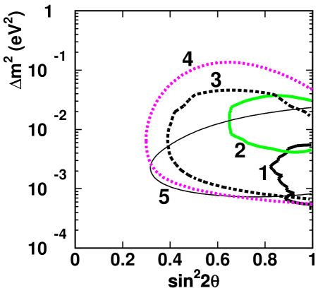
Figure 30: Constraints on $\nu_{\mu}-\nu_{\tau}$ mixing from (1,2) contained events in super-Kamiokande and Kamiokande, (3,4) upward-going muons in super-Kamiokande and Kamiokande, and (5) stop/through upward muons in super-Kamiokande [115].

but is this compatible with the large mixing indicated (at least) for atmospheric neutrinos? Indeed it is [116], and theoretically it is difficult to see why any pair of neutrinos should be almost degenerate. On the other hand, there are perfectly natural $2\times 2$ light-neutrino mass matrices that are compatible with large $\sin^{2}2\theta_{\mu\tau}$ and the first mass hierarchy in (136) if $m_{\nu_{2}}\sim\sqrt{\Delta m^{2}_{S}}\sim 10^{-2^{1/2}}$ eV, particularly when it is observed [117] that renormalization-group effects below $M_{GUT}$ may enhance $\sin^{2}2\theta_{\mu\tau}$, as seen in Fig. 31 [116]. However, it is very difficult to understand the much larger hierarchy that would be needed for the vacuum solution to the solar neutrino problem with $m_{\nu_{2}}\sim\sqrt{\Delta m^{2}_{S}}\sim 10^{-5}$ eV. It is a more model-dependent question whether the large- or small-angle MSW solution is favoured. In one particular GUT model [116], we found the large-angle MSW solution more plausible, but the small-angle MSW solution could not be excluded. We still need more experimental information on neutrino masses and mixing, and this will surely be an active experimental field for years to come.

Figure 31: Possible renormalization-group effect on the mixing angle in a two-generation neutrino model with supersymmetry at large $\tan\beta$ [116].

5 NONE OF THE ABOVE

Now is a good moment to review the progress made in addressing the defects of the Standard Model that were reviewed in Lecture 1, and to count how many parameters are still free. Grand unification reduces the three independent gauge couplings of the Standard Model to just one, so that is certainly progress. As far as the Standard Model Higgs sector is concerned, supersymmetry fixes the quartic Higgs coupling, which is progress, but the overall scale of electroweak gauge symmetry breaking is related to the undetermined scale of supersymmetry breaking. Indeed, in the absence of further theoretical input, the soft supersymmetry-breaking mass introduces ${\cal O}(100)$ new parameters unless (why?) one knows how to impose flavour universality.

Moreover, a complete treatment of neutrino masses involves additional parameters to describe the GUT Higgs potential [91, 61] and a see-saw mass matrix [110]. What is more, we still need at least one parameter to generate the cosmological baryon asymmetry and another to generate cosmological inflation. Finally, we should not forget gravity, whose parameters include the cosmological constant (if it vanishes, we need to understand why) as well as Newton’s constant.

Thus, although progress has been made, there remain big questions in the supersymmetry-breaking sector and in quantum gravity, which are the main subjects addressed in this Lecture.

5.1 Supersymmetry Breaking

It is clear that supersymmetry must be broken: $m_{\tilde{e}}\neq m_{e},m_{\tilde{\gamma}}\neq m_{\gamma}=0$, etc. Could it be explicit or must it be spontaneous? Explicit supersymmetry breaking is not only ugly and unlike what occurs in gauge theories, it also induces inconsistencies at the quantum level when gravity is introduced. Therefore, attention has focused on spontaneous symmetry breaking. Since the supersymmetry charge $Q$ is fermionic, this requires a non-zero matrix element for $Q$ between the vacuum and some fermion $\chi$ called a Goldstone fermion or Goldstino:

$$<0|Q|\chi>=f^{2}_{\chi}\not=0$$ (137)

The non-zero matrix element (137) has the immediate consequence, within global supersymmetry, that the vacuum energy is necessarily positive. This follows from the basic supersymmetry algebra:

$$\{Q,Q\}\propto\gamma_{\mu}P^{\mu}$$ (138)

Sandwiching (138) between vacuum states and inserting the intermediate state $|\chi><\chi|$, we find

$$|<0|Q|\chi>|^{2}=f^{4}_{\chi}>0$$ (139)

and hence the vacuum energy

$$<0|P_{0}|0>\equiv E_{0}>0$$ (140)

How may this spontaneous symmetry breaking be achieved? We recall the general form of the effective scalar potential in a globally supersymmetric theory:

$$V=\sum_{i}\left|\frac{\partial W}{\partial\phi^{i}}\right|^{2}+\frac{1}{2}\sum_{\alpha}\;g^{2}_{\alpha}|\phi^{*}T^{\alpha}\phi|^{2}$$ (141)

where the former is called the $F$ term and the latter the $D$ term. In order to obtain (140), we need either the first term to be non-zero “$F$-breaking” [118] - or the second term - “$D$-breaking” [119]. The latter would require an extra U(1) gauge group factor and many new matter fields, so we illustrate global supersymmetry breaking with the simplest $F$-breaking model [118].

Consider the superpotential

$$W=\alpha AB^{2}+\beta C(B^{2}-m^{2})$$ (142)

where $A,B,C$ denote gauge-singlet matter supermultiplets. It is easy to see that (142) yields

$$F^{\dagger}_{A}=\alpha B^{2},~{}~{}~{}F^{\dagger}_{B}=2B(\alpha A+\beta C),~{}~{}~{}F^{\dagger}_{C}=\beta(B^{2}-m^{2})$$ (143)

and hence an effective scalar potential

$$V=\sum_{i=A,B,C}\,|F_{i}|^{2}=|2B(\alpha A+\beta C)|^{2}+|\alpha B^{2}|^{2}+\beta(B^{2}-m^{2})|^{2}$$ (144)

It is apparent that the last two terms cannot vanish simultaneously, so that $V>0$ and supersymmetry is broken.

Recently there have been analyses of high-redshift supernovae [120] and other astrophysical and cosmological data [121] that favour a non-zero cosmological constant, as would be suggested by such positive vacuum energy. Unfortunately, the model (142) and others like it are too much of a good thing. The “observed” cosmological constant, if it is real at all, would correspond to

$$\Lambda\mathrel{\hbox to0.0pt{\raise 2.15277pt\hbox{$<$}\hss}{\lower 2.15277pt\hbox{$\sim$}}}10^{-123}m^{4}_{P}$$ (145)

whereas such a global model of supersymmetry breaking would correspond to

$$\Lambda\sim(1\;TeV)^{4}\sim 10^{-64}\,m^{4}_{P},$$ (146)

a discrepancy by some 60 orders of magnitude! Even the QCD vacuum energy

$$E_{QCD}\sim(100\,MeV)^{4}\sim 10^{-80}\,m^{4}_{P}$$ (147)

is much larger than the ”observed” value (145). This discrepancy may be the biggest problem in theoretical physics, even bigger than the hierarchy problem. However, to address it requires a true quantum theory of gravity, as is discussed later in this lecture.

However, before doing so, let us briefly review the latest incarnation of global supersymmetry-breaking models, namely gauge-mediated or messenger models [66]. The basic idea is to hide the ugly origin of supersymmetry breaking in a hidden sector of the theory that is coupled to observable particles via an intermediate set of “messenger” particles that share some of the gauge interactions of the Standard Model, as seen in Fig. 32. Gauge interactions then mediate the supersymmetry breaking needed in the observable sector. These models were originally conceived in the early 1980’s [122] because neither the $F$-breaking scenario (142) nor $D$-breaking models fitted within the MSSM. They have recently been reincarnated [123] with the idea that supersymmetry breaking in the hidden sector might originate from non-perturbative phenomena, which are much better understood by now [66].

Figure 32: Sketch of the principle of gauge-mediated (messenger) models: supersymmetry breaking in a hidden sector is communicated to the observable sector via gauge interactions [66].

There have been two principal motivations for this reincarnation. One is that gauge mediation naturally imposes flavour universality in the observable sector [123]. All quarks (or leptons) with the same charge acquire universal soft supersymmetry-breaking scalar masses, avoiding any problems with flavour-changing neutral interactions [65] and reducing the effective number of parameters in the observable sector. A feature of gauge-mediated models is the appearance of a massless Goldstone fermion $\lambda$, which would acquire a small mass when gravity is taken into account, as discussed in the next section. This implies that the lightest neutralino $\chi$ is unstable: $\chi\to\lambda\gamma$ decay dominates.

This provides the second motivation for gauge-mediated models, which is the report by the CDF collaboration [124] of an apparent $\bar{p}p\to e^{+}e^{-}\gamma\gamma+$ missing $p_{T}$ event. It has been suggested [125] that this might be due to $\tilde{e}^{+}\tilde{e}^{-}$ pair production followed by $\tilde{e}^{\pm}\to e^{\pm}\chi,\,\chi\to\lambda\gamma$ decays, or due to $\chi^{+}\chi^{-}$ pair production followed by $\chi^{\pm}\to e^{\pm}\nu\chi,\,\chi\to\lambda\gamma$ decays. However, no other $\gamma\gamma+$ missing $p_{T}$ events have been observed either at LEP [16] or at the FNAL Tevatron collider [126], and most of the parameter spaces for these interpretations have now been excluded, as seen in Fig. 33 [16]. Clearly, further experimental input from future collider runs is needed.

Figure 33: Region of the $(m_{\tilde{e}},m_{\chi})$ plane excluded by LEP [16] in models with a light gravitino, compared with the region favoured in the $\bar{p}p\rightarrow\tilde{e}\tilde{\bar{e}}+X$ interpretation [125] of the CDF $\bar{p}p\rightarrow e^{+}e^{-}\gamma\gamma p\hbox to0.0pt{\hss$/$}_{T}+X$ event [124].

Some final comments on gauge-mediated models are in order. The first is that it has proved to be quite difficult to construct a model that is consistent with all the phenomenological constraints, has a desirable stable vacuum, etc. . The other is that, to the extent that the hidden scale $\Lambda_{H}\gg 1\,\mbox{TeV}$, the apparent vacuum energy (cosmological constant) $\sim\Lambda^{4}_{H}\gg 10^{-64}\,m^{4}_{P}$, worsening the discrepancy with the astrophysical upper limit (or observation) (145). However, in order to discuss this issue seriously, one needs a supersymmetric quantum theory of gravity, to which we now turn.

5.2 Local Supersymmetry and Supergravity

Why make a local theory of supersymmetry? One motivation is the analogy with gauge theories, in which bosonic symmetries are made local. Another is that local supersymmetry necessarily involves the introduction of gravity. Since both gravity and (surely!) supersymmetry exist, this seems an inevitable step. It also leads to the possibility of unifying all the particle interactions including gravity, which was one of our original motivations for supersymmetry. Moreover, in the context of this Lecture, it is interesting that local supersymmetry (supergravity) admits an elegant mechanism for supersymmetry breaking [127], analogous to the Higgs mechanism in gauge theories, which allows us to address more seriously the possible existence of a cosmological constant.

The basic building block in a supergravity theory [45, 46] is the graviton supermultiplet of (51), which contains particles with helicities $(2,3/2)$, the latter being the gravitino of spin $3/2$. Why is this required when one makes supersymmetry local?

We recall the basic global supersymmetry transformation laws (54) for bosons and fermions. Consider now the combination of two such global supersymmetry transformations:

$$[\delta_{1},\delta_{2}]~{}(\phi\,~{}\mbox{or}~{}\,\psi)=-(\bar{\xi}_{2}\gamma_{\mu}\xi_{1})~{}(i\,\partial_{\mu})~{}(\phi\,~{}\mbox{or}~{}\,\psi)+\ldots$$ (148)

The operator $(i\,\partial_{\mu})$ corresponds to the momentum $P_{\mu}$, and we see again that the combination of two global supersymmetry transformations is a translation. Consider now what happens when we consider local supersymmetry transformations characterized by a varying spinor $\xi(x)$. It is evident that the infinitesimal translation $\bar{\xi}_{2}\gamma^{\mu}\xi_{1}$ in (148) is now $x$-dependent, and the previous global translation becomes a local coordinate transformation, as occurs in General Relativity.

How do we make the theory invariant under such local supersymmetry transformations? Consider again the simplest globally supersymmetric model containing a free spin-1/2 fermion and a free spin-0 boson (53), and make the local versions of the transformations (54). Following the same steps as in Lecture 2, we find that

$$\delta{\cal L}=\partial_{\mu}(\cdots)+2\bar{\psi}\gamma_{\mu}\,\partial\hbox to0.0pt{\hss$/$}S(\partial^{\mu}\xi(x))+\mbox{herm. conj.}$$ (149)

In contrast to the global case, the action $A=\int d^{4}x{\cal L}$ is not invariant, because of the second term in (149). To cancel it out and restore invariance, we need more fields.

We proceed by analogy with gauge theories. In order to make the kinetic term $(i\bar{\psi}\partial\hbox to0.0pt{\hss$/$}\psi)$ invariant under gauge transformations $\psi\to e^{i\epsilon(x)}\psi$, we need to cancel a variation

$$-\bar{\psi}\partial_{\mu}\psi\partial^{\mu}\epsilon(x)$$ (150)

which is done by introducing a coupling to a gauge boson:

$$g\bar{\psi}\gamma_{\mu}\psi A^{\mu}(x)$$ (151)

and the corresponding transformation:

$$\delta A_{\mu}(x)=\frac{1}{g}\partial_{\mu}\epsilon(x)$$ (152)

In the supersymmetric case, we cancel the second term in (149) by a coupling:

$$\kappa\bar{\psi}\gamma_{\mu}\partial\hbox to0.0pt{\hss$/$}S\psi^{\mu}(x)$$ (153)

to a spin-3/2 spinor $\psi^{\mu}(x)$, representing a gauge fermion or gravitino, with the corresponding transformation:

$$\delta\psi^{\mu}=-\frac{2}{\kappa}\,\partial^{\mu}\xi(x)$$ (154)

where $\kappa\equiv 8\pi/m^{2}_{P}$.

For completeness, let us at least write down the Lagrangian for the graviton-gravitino supermultiplet:

$$L=-\frac{1}{2\kappa^{2}}\,\sqrt{-g}R-\frac{1}{2}\,\epsilon^{\mu\nu\rho\sigma}\bar{\psi}_{\mu}\gamma_{5}\gamma_{\nu}{\cal D}_{\rho}\psi_{\sigma}$$ (155)

where $g$ denotes the determinant of the metric tensor:

$$g_{\mu\nu}=\epsilon^{m}_{\mu}\eta_{mn}\epsilon^{\mu}_{\nu}$$ (156)

where $\epsilon^{m}_{\mu}$ is the vierbein and $\eta_{mn}$ the Minkowski metric tensor, and ${\cal D_{\rho}}$ is a covariant derivative

$${\cal D_{\rho}}\equiv\partial_{\rho}+\frac{1}{4}\,\omega^{mn}_{\rho}[\gamma_{m},\gamma_{n}]$$ (157)

where $\omega^{mn}_{\rho}$ is the spin connection. This is the simplest possible generally-covariant model of a spin-3/2 field. It is remarkable that it is invariant under the local supersymmetry transformations:

$$\delta\epsilon^{m}_{\mu} = \frac{x}{2}\,\bar{\xi}(x)\gamma^{m}\psi_{\mu}(x),$$

$$\delta\omega_{\mu}^{mn} = 0,\delta\psi_{\mu}=\frac{1}{x}\,{\cal D}_{\mu}\xi(x)$$ (158)

just as the simplest possible $(1/2,0)$ theory (53) was globally supersymmetric, and also the action of an adjoint spin-1/2 field in a gauge theory.

It is also remarkable that supergravity admits an elegant analogue of the Higgs mechanism of spontaneous symmetry breaking [127]. Just as one combines the two polarization states of a massless gauge field with the single state of a massless Goldstone boson to obtain the three polarization states of a massive gauge boson, one may combine the two polarization states of a massless gravitino $\psi_{\mu}$ with the two polarization states of a massless Goldstone fermion $\lambda$ to obtain the four polarization states of a massive spin-3/2 particle $\tilde{G}$. This super-Higgs mechanism corresponds to a spontaneous breakdown of local supersymmetry, since the massless graviton $G$ has a different mass from the gravitino $\tilde{G}$:

$$m_{G}=0\not=m_{\tilde{G}}.$$ (159)

This is the only known consistent way of breaking local symmetry, just as the Higgs mechanism is the only way to generate $m_{W}\not=0$.

Moreover, this can be achieved while keeping zero vacuum energy (cosmological constant), at least at the tree level. The reason for this is the appearance in local supersymmetry (supergravity) of a third term in the effective potential (141), which has a negative sign [127]. There is no time in these lectures to discuss this exciting feature in detail: the interested reader is referred to the original literature and the simplest example [128]. In this latter case, $\Lambda=V=0$ for any value of the gravitino mass, for which reason it was named no-scale supergravity [129].

Again, there is no time to discuss here details of the coupling of supergravity to matter [127]. However, it is useful to have in mind the general features of the theory in the limit where $\kappa\to 0$, but the gravitino mass $m_{\tilde{G}}\equiv m_{3/2}$ remains fixed. One generally has non-zero gaugino masses $m_{1/2}\propto m_{3/2}$, and their universality is quite generic. One also has non-zero scalar masses $m_{0}\propto m_{3/2}$, but their universality is much more problematic, and even violated in generic string models. It was this failing that partly refuelled the renewed interest in the gauge-mediated models mentioned in the previous section. A generic supergravity theory also yields non-universal trilinear soft supersymmetry-breaking couplings $A_{\lambda}\lambda\phi^{3}:A_{\lambda}\propto m_{3/2}$ and bilinear scalar couplings $B_{\mu}\mu\phi^{2}:B_{\mu}\propto m_{3/2}$. Therefore, supergravity may generate the full menagerie of soft supersymmetry-breaking terms:

$$-\frac{1}{2}\,\sum_{a}\,m_{1/2_{a}}\,\tilde{V}_{a}\tilde{V}_{a}-\sum_{i}\,m^{2}_{0_{i}}|\phi_{i}|^{2}-(\sum_{\lambda}A_{\lambda}\lambda\phi^{3}+\mbox{h.c.})-(\sum_{\mu}B_{\mu}\mu\phi^{2}+\mbox{h.c.})$$ (160)

Since these are generated at the supergravity scale near $m_{P}\sim 10^{19}$ GeV, the soft supersymmetry-breaking parameters are renormalized as discussed in Lecture 2. The analogous parameters in gauge-mediated models would also be renormalized, but to a different extent, because the mediation scale $\ll m_{P}$. This difference may provide a signature of such models, as discussed elsewhere [130].

Also renormalized is the vacuum energy (cosmological constant), which is a potential embarassment. Loop corrections in a non-supersymmetric theory are quartically divergent, whereas those in a generic supergravity theory are only quadratically divergent, suggesting a contribution to the cosmological constant of order $m^{2}_{3/2}m^{2}_{P}$, perhaps $O(10^{-32})m^{4}_{P}$! Particular models may have a one-loop quantum correction of order $m^{4}_{3/2}=O(10^{-64})m^{2}_{P}$, but more magic (a new symmetry?) is needed to suppress the cosmological constant to the required level (145). This is one of the motivations for tackling string theory, which is our only candidate for a fundamental Theory of Everything including gravity.

5.3 Problems of Gravity

The greatest piece of unfinished business for twentieth-century physics is to reconcile general relativity with quantum mechanics. There are aspects of this problem, one being that of the cosmological constant, as discussed above. Another is that of perturbative quantum-gravity effects. Tree-level graviton exchange in $2\to 2$ scattering, such as $e^{+}e^{-}\to e^{+}e^{-}$ at LEP, has an amplitude $A_{G}\sim E^{2}/m^{2}_{P}$, and hence a cross section

$$\sigma_{G}\sim E^{2}/m^{4}_{P}$$ (161)

This is very small (negligible!) at LEP energies, reaching the unitarity limit only when $E\sim m_{P}$. However, when one calculates loop amplitudes involving gravitons, the rapid growth with energy (161) leads to uncontrollable, non-renormalizable divergences. These are of power type, and diverge faster and faster in higher orders of perturbation theory.

There are also non-perturbative problems in the quantization of gravity, that first arose in connection with black holes. From the pioneering work of Bekenstein and Hawking [131] on black-hole thermodynamics, we know that black holes have non-zero entropy $S$ and temperature $T$, related to the Schwarzschild horizon radius. This means that the quantum description of a black hole should involve mixed states. The intuition underlying this feature is that information can be lost through the event horizon. Consider, for example, a pure quantum-mechanical pair state $|A,B>\equiv\sum_{i}c_{i}|A_{i}>|B_{i}>$ prepared near the horizon, and what happens if one of the particles, say $A$, falls through the horizon while $B$ escapes, as seen in Fig. 34. In this case,

$$\sum_{i}\,c_{i}|A_{i}B_{i}>\to\sum_{i}|c_{i}|^{2}|B_{i}><B_{i}|$$ (162)

and $B$ emerges in a mixed state, as in Hawking’s original treatment of the black-hole radiation that bears his name [131].

Figure 34: If a pair of particles $|A>~{}|B>$ is produced near the horizon of a black hole, and one of them ($|A>$, say) falls in, the remaining particle $|B>$ will appear to be in a mixed state.

The problem is that conventional quantum mechanics does not permit the evolution of a pure initial state into a mixed final state. This is an issue both for the quantum particles discussed above and for the black hole itself. We could imagine having prepared the black hole by fusing massive or energetic particles in a pure initial state, e.g., by splitting a laser beam and then firing the sub-beams at each other as in a laser device for inertial nuclear fusion.

These problems point to a fundamental conflict between the proudest achievements of early twentieth-century physics, quantum mechanics and general relativity. One or the other should be modified, and perhaps both. Since quantum mechanics is sacred to field theorists, most particle physicists prefer to modify General Relativity by elevating it to string theory [30].

5.4 Introduction to String Theory

At the level of perturbation theory, the divergence difficulties of quantum gravity can be related to the absence in a point-particle theory of a cutoff at short distances: for example,

$$\int^{\Lambda\to\infty}\,d^{4}k\left(\frac{1}{k^{2}}\right)\leftrightarrow\int_{1/\Lambda\to 0}\,d^{4}x\left(\frac{1}{x^{6}}\right)\sim\Lambda^{2}\to\infty$$ (163)

Such divergences can be alleviated or removed if one replaces point particles by extended objects. The simplest possibility is to extend in just one dimension, leading us to a theory of strings. In such a theory, instead of point particles describing one-dimensional world lines, we have strings describing two-dimensional world sheets. Most popular have been closed loops of string, whose simplest world sheet is a tube. The “wiring diagrams” generated by the Feynman rules of conventional point-like particle theories become the “plumbing circuits” generated by the junctions and connections of these tubes of closed string. One could imagine generalizing this idea to higher-dimensional extended objects such as membranes describing world volumes, etc., and we return later to this option.

On a historical note, string models first arose from old-fashioned strong-interaction theory, before the advent of QCD. The lowest-lying hadronic states were joined by a very large number of excited states with increasing masses $m$ and spins $J$:

$$J=\alpha^{\prime}m^{2}$$

where $\alpha^{\prime}$ was called the “Regge slope”. One interpretation of this spectrum was of $\bar{q}q$ bound states in a linearly-rising potential, like an elastic string holding the constituents together, with tension $\mu=1/\alpha^{\prime}$. It was pointed out that such an infinitely (?) large set of resonances in the direct $s$-channel of a scattering process could be dual (equivalent) to the exchange of a similar infinite set in the crossed channel. Mathematically, this idea was expressed by the Veneziano [133] amplitude for $2\to 2$ scattering, and its generalizations to $2\to n$ particle production processes. Then it was pointed out that these amplitudes could be derived formally from an underlying quantum theory of string [134]. However, this first incarnation of string theory was not able to accommodate the point-like partons seen inside hadrons at this time - the converse of the quantum-gravity motivation for string theory mentioned at the beginning of this section. Then along came QCD, which incorporated these point-like scaling properties and provided a qualitative understanding of confinement, which has now become quantitative with the advent of modern lattice calculations. Thus string theory languished as a candidate model of the strong interactions.

It was realized early on that unitarity required the existence of closed strings, even in an a priori open-string theory. Moreover, it was observed that the spectrum of a closed string included a massless spin-2 particle, which was an embarrassment for a theory of the strong interactions. However, this led to the idea [135] of reinterpreting string theory as a Theory of Everything, with this massless spin-2 state interpreted as the graviton and the string tension elevated to $\mu=O(m^{2}_{P})$.

As already mentioned, one of the primary reasons for studying extended objects in connection with quantum gravity is the softening of divergences associated with short-distance behaviour. Since the string propagates on a world sheet, the basic formalism is two-dimensional. Accordingly, string vibrations may be described in terms of left- and right-moving waves:

$$\phi(r,t)\to\phi_{L}(r-t),\,\phi_{R}(r+t)$$ (164)

If the string has no boundary, as for a closed string, the left- and right-movers are independent. When quantized, they may be described by a two-dimensional field theory. Compared to a four-dimensional theory, it is relatively easy to make a two-dimensional field theroy finite. In this case, it has conformal symmetry, which has an infinite-dimensional symmetry group in two dimensions. However, as you already know from gauge theories, one must be careful to ensure that this classical symmetry is not broken at the quantum level by anomalies. If the quantum string theory is to be consistent in a flat background space-time, the conformal anomaly fixes the number of left- and right-movers each to be equivalent to 26 free bosons if the theory has no supersymmetry, or 10 boson/fermion supermultiplets if the theory has $N=1$ supersymmetry on the world sheet. There are other important quantum consistency conditions, and it was the demonstration by Green and Schwarz [136] that certain string theories are completely anomaly-free that opened the floodgates of theoretical interest in string theory as a Theory of Everything [30].

Among consistent string theories, one may enumerate the following. The Bosonic String exists in 26 dimensions, but this is not even its worst problem! It contains no fermionic matter degrees of freedom, and the flat-space vacuum is intrinsically unstable. Superstrings exist in 10 dimensions, have fermionic matter and also a stable flat-space vacuum. On the other hand, the ten-dimensional theory is left-right symmetric, and the incorporation of parity violation in four dimensions is not trivial. The Heterotic String [137] was originally formulated in 10 dimensions, with parity violation already incorporated, since the left- and right movers were treated differently. This theory also has a stable vacuum, but suffers from the disadvantage of having too many dimensions. Four-Dimensional Heterotic Strings may be obtained either by compactifying the six surplus dimensions: $10=4+6$ compact dimensions with size $R\sim 1/m_{P}$ [138], or by direct construction in four dimensions, replacing the missing dimensions by other internal degrees of freedom such as fermions [139] or group manifolds or …? In this way it was possible to incorporate a GUT-like gauge group [99] or even something resembling the Standard Model [140].

What are the general features of such string models? First, they predict there are no more than 10 dimensions, which agrees with the observed number of 4! Secondly, they suggest that the rank of the four-dimensional gauge group should not be very large, in agreement with the rank 4 of the Standard Model! Thirdly, the simplest four-dimensional string models do not accommodate large matter representations [141], such as an 8 of SU(3) or a 3 of SU(2), again in agreement with the known representation structure of the Standard Model! Fourthly, simple string models predict fairly successfully the mass of the top quark. This is because the maximum generic value of a Yukawa coupling $\lambda_{t}$ is of the same order as the gauge coupling $g$. Applied to the top quark, this suggests that

$$m_{t}=\lambda_{t}<0|H|0>=O(g)\times 250\mbox{GeV}$$ (165)

Moreover, the renormalization-group equation for $\lambda_{t}$ exhibits an approximate infra-red fixed point, as seen in Fig. 35. This means that a large range of Yukawa coupling inputs at the Planck scale yield very similar physical values of $m_{t}\mathrel{\hbox to0.0pt{\raise 2.15277pt\hbox{$<$}\hss}{\lower 2.15277pt\hbox{$\sim$}}}$ 190 GeV. Fifthly, string theory makes a fairly successful prediction for the gauge unification scale in terms of $m_{P}$. If the intrinsic string coupling $g_{s}$ is weak, one predicts [142]

Figure 35: The approximate infra-red fixed point of the renormalization-group equation for $m_{t}$ means that a wide range of input Yukawa couplings at the GUT or string scale lead to similar physical values of $m_{t}\mathrel{\hbox to0.0pt{\raise 2.15277pt\hbox{$<$}\hss}{\lower 2.15277pt\hbox{$\sim$}}}$ 190 GeV.

$$M_{GUT}=O(g)\times\frac{m_{P}}{\sqrt{8\pi}}\simeq\mbox{few}\times 10^{17}\mbox{GeV}$$ (166)

where $g$ is the gauge coupling, which is ${\cal O}(20)$ higher than the value calculated from the bottom up in Lecture 4 on the basis of LEP measurement of the gauge couplings. On the one hand, it is impressive that the bottom-up extrapolation over 14 decades agrees to within 10 % (on a logarithmic scale) with the top-down calculation (165). Nevertheless, it would be nice to obtain closer agreement, and this provides the major motivation for considering strongly-coupled string theory, which corresponds to a large internal dimension $l>m^{-1}_{GUT}$, as we discuss next.

5.5 Beyond String

Current developments involve going beyond string to consider higher-dimensional extended objects, such as generalized membranes with various numbers of internal dimensions. These may be obtained as solitons (non-perturbative classical solutions) of string theory, with masses

$$m\propto{1\over g_{s}}$$ (167)

analogously to monopoles in gauge theory. It is evident from (167) that such membrane-solitons become light in the limit of strong string coupling $g_{s}\to\infty$.

It was observed some time ago that there should be a strong-coupling/weak-coupling duality [143] between elementary excitations and monopoles in supersymmetric gauge theories. These ideas have recently been confirmed in a spectacular solution of $N=2$ supersymmetric gauge theory in four dimensions [144]. Similarly, it has recently been shown that there are analogous dualities in string theory, whereby solitons in some strongly-coupled string theory are equivalent to light string states in some other weakly-coupled string theory. Indeed, it appears that all string theories are related by such dualities. A particularity of this discovery is that the string coupling strength $g_{s}$ is related to an extra dimension, in such a way that its size $R\to\infty$ as $g_{s}\to\infty$. This then leads to the idea of an underlying 11-dimensional framework called $M$ theory [145] that reduces to the different string theories in different strong/weak-coupling linits, and reduces to eleven-dimensional supergravity in the low-energy limit.

A particular class of string solitons called $D$-branes [146] offers a promising approach to the black hole information paradox mentioned previously. According to this picture, black holes are viewed as solitonic balls of string, and their entropy simply counts the number of internal string states [132, 147]. These are in principle countable, so string theory may provide an accounting system for the information contained in black holes. Within this framework, the previously paradoxical process (162) becomes

$$|A,B>+|BH>\to|B^{\prime}>+|BH^{\prime}>$$ (168)

and the final state is pure if the initial state was. The apparent entropy of the final state in (162) is now interpreted as entanglement. The “lost” information is in principle encoded in the black-hole state, and this information could be extracted if we measured all properties of this ball of string.

In practice, we do not know how to recover this information from macroscopic black holes, so they appear to us as mixed states. What about microscopic black holes, namely fluctuations in the space-time background with $\Delta E=O(m_{P})$, that last for a period $\Delta t=O(1/m_{P})$ and have a size $\Delta x=O(1/m_{P})$? Do these steal information from us [148], or do they give it back to us when they decay? Most people think there is no microscopic leakage of information in this way, but not all of us [132] are convinced. The neutral kaon system is among the most sensitive experimental areas [149, 150, 151] for testing this speculative possibility.

A final experimental comment concerns the magnitude of the extra dimension in $M$ theory: LEP data suggest that it may be relatively large, with size $L_{11}\gg 1/m_{GUT}\simeq 1/10^{16}~{}\mbox{GeV}\gg 1/m_{P}$ [152]. Remember that the naïve string unification scale (166) is about 20 times larger than $m_{GUT}$. This may be traced to the fact that the gravitational interaction strength, although growing rapidly as a power of energy (161), is still much smaller than the gauge coupling strength at $E=m_{GUT}$. However, if an extra space-time dimension appears at an energy $E<m_{GUT}$, the gravitational interaction strength grows fast, as indicated in Fig. 36. Unification with gravity around $10^{16}\mbox{GeV}$ then becomes possible, if the gauge couplings do not also acquire a similar higher-dimensional kick. Thus we are led to the startling capacitor-plate framework for fundamental physics shown in Fig. 37.

Figure 36: Sketch of the possible evolution of the gauge couplings and the gravitational coupling $G$: if there is a large fifth dimension with size $\gg m^{-1}_{GUT}$, $G$ may be unified with the gauge couplings at the GUT scale.

Figure 37: The capacitor-plate scenario favoured in eleven-dimansional $M$ theory. The eleventh dimension has a size $L_{11}\gg M_{GUT}^{-1}$, whereas dimensions $5,...,10$ are compactified on a small manifold $K$ with characteristic size $\sim M_{GUT}^{-1}$. the remaining four dimensions form (approximately) a flat Minkowski space $M_{4}$.

Each plate is a priori ten-dimensional, and the bulk space between then is a priori eleven-dimensional. Six dimensions are compactified on a scale $L_{6}\sim 1/m_{GUT}$, leaving a theory which is effectively five-dimensional in the bulk and four-dimensional on the walls. Conventional gauge interactions and observable matter particles are hypothesized to live on one capacitor plate, and there are other hidden gauge interactions and matter particles living on the other plate. The fifth dimension has a characteristic size which is estimated to be $O(10^{12}~{}\mbox{to}~{}10^{13}~{}\mbox{GeV})^{-1}$, and physics at large distances (smaller energies) looks effectively four-dimensional. Supersymmetry breaking is expected to originate on the hidden capacitor plate in this scenario, and to be transmitted to the observable wall by gravitational strength interactions in the bulk [153].

The phenomenological richness of this speculative $M$-theory approach is only beginning to be explored, and it remains to be seen whether it offers a realistic phenomenological description. However, it does embody all the available theoretical wisdom as well as offering the prospect of unifying all the observable gauge interactions with gravity at a single effective scale $\sim m_{GUT}$. As such, it constitutes our best contemporary guess about the Theory of Everything within and Beyond the Standard Model.

References

-
[1]
S.L. Glashow, Nucl.Phys. 22 (1961) 579;
S. Weinberg, Phys.Rev.Lett. 19 (1967) 1264;
A. Salam, Proc. 8th Nobel Symposium, Stockholm 1968, ed. N. Svartholm (Almqvist and Wiksells, Stockholm, 1968), p. 367. - [2] Super-Kamiokande collaboration, Y. Fukuda et al., Phys.Rev.Lett. 81 (1998) 1562.
- [3] C. Quigg, Gauge Theories of the Strong, Weak and Electromagnetic Interactions (Benjamin-Cummings, Reading, 1983).
- [4] D. Ross and M. Veltman, Nucl.Phys. B95 (1975) 135.
-
[5]
M. Grünewald and D. Karlen, talks at International
Conference on High-Energy Physics, Vancouver 1998,
http://www.cern.ch/LEPEWWG/misc. - [6] C. Bouchiat, J. Iliopoulos and Ph. Meyer, Phys.Lett. 138B (1972) 652 and references therein.
- [7] H. Georgi, H. Quinn and S. Weinberg, Phys.Rev.Lett. 33 (1974) 451.
- [8] H. Georgi and S.L. Glashow, Phys.Rev.Lett. 32 (1974) 438.
-
[9]
S. Dimopoulos and H. Georgi, Nucl.Phys. B193 (1981)
50;
S. Dimopoulos, S. Raby and F. Wilczek, Phys.Rev. D24 (1981) 1681;
L. Ibàñez and G.G. Ross, Phys.Lett. 105B (1981) 439. -
[10]
J.S. Bell, Nucl.Phys. 60 (1973) 427;
C.H. Llewellyn Smith, Phys.Lett. 46B (1973) 233;
J. Cornwall, D. Levin and G. Tiktopoulos, Phys.Rev.Lett. 30 (1973) 1268. - [11] J. Ellis, M.K. Gaillard and D.V. Nanopoulos, Nucl.Phys. B106 (1976) 292.
-
[12]
M. Veltman, Acta Phys.Pol. B8 (1977) 475;
C. Vayonakis, Lett.Nuovo Cimento 17 (1976) 383. - [13] B.W. Lee, C. Quigg and H.B. Thacker, Phys.Rev. D16 (1977) 1519.
- [14] L. Durand and J. Lopez, Phys.Rev.Lett. 64 (1990) 1215 and Phys.Rev. D45 (1992) 3112.
- [15] B.L. Ioffe and V.A. Khoze, Sov.J.Part.Nucl. 9 (1978) 50.
-
[16]
LEP Experiments Committee meeting, Nov. 12th, 1998,
http:www.cern.ch/Committees/LEPC/minutes/LEPC50.html.
This source provides some preliminary updates of experimental plots reproduced in these notes, which are mainly taken from papers contributed to the International Conference on High-Energy Physics, Vancouver 1998:
http://ichep.triumf.ca/main.asp. -
[17]
G. Altarelli, R. Kleiss and C. Verzegnassi, eds.,
Physics at
LEP 1, CERN Report 89-08 (1989);
D. Bardin, W. Hollik and G. Passarino, eds., Reports of the Working Group on Precision Calculations for the Z Resonance, CERN Report 95-03 (1995). - [18] M. Davier and A. Hocker, Phys.Lett. 435 (1998) 427.
- [19] A. Sirlin, Phys.Rev. D22 (1980) 971, Nucl.Phys. B332 (1990) 20 and Phys.Lett. B267 (1991) 240.
-
[20]
M. Veltman, Nucl.Phys. 123 (1977) 89;
M.S. Chanowitz, M. Furman and I. Hinchliffe, Phys.Lett. B78 (1978) 285. - [21] M. Veltman, Acta Phys.Pol. 8 (1977) 475.
- [22] U. Amaldi et al., Phys.Rev. D36 (1987) 1385
- [23] G. Costa et al., Nucl.Phys. B297 (1988) 244.
- [24] Particle Data Group, C. Caso et al., Eur.Phys.J. C3 (1998) 1.
- [25] G. Altarelli, T. Sjöstrand and F. Zwirner, eds., Proceedings of the Workshop on Physics at LEP 2, CERN Report 96-01 (1996).
- [26] J. Ellis, G.L. Fogli and E. Lisi, Phys.Lett. B318 (1993) 148; Phys.Lett. B333 (1994) 118; Zeit.Phys. C69 (1996) 627 and Phys.Lett. B389 (1996) 321.
- [27] Y.F. Pirogov and O.V. Zenin, hep-ph/9808396.
- [28] P. Hasenfratz and J. Nager, Zeit.Phys. C37 (1988) 477.
- [29] Y. Nir, lectures at this school.
- [30] M.B. Green, lectures at this school.
-
[31]
Y. Nambu, in: Z. Ajduk, S. Pokorski and A. Trautman, eds.,
Proc. XI Int. Symp. on Elementary Particle Physics (World
Scientific,
Singapore, 1989);
A. Miranski, M. Tanabashi and K. Yamauraki, Mod.Phys.Lett A4 (1989) 1043 and Phys.Lett. B221 (1989) 177. -
[32]
W.A. Bardeen, C.T. Hill and M. Lindner, Phys.Rev. D41 (1990) 1647;
For a review, see: E. Farhi and L. Susskind, Phys.Rep. 74C (1981) 277. -
[33]
S. Dimopoulos and L. Susskind, Nucl.Phys. B155 (1979) 237;
E. Eichten and K. Lane, Phys.Lett. B90 (1980) 125. - [34] M.E. Peskin and T. Takeuchi, Phys.Rev. D46 (1992) 381.
-
[35]
G. Altarelli, R. Barbieri and S. Jadach, Nucl.Phys. B369 (1992) 3;
376 (1992) 444 (E);
G. Altarelli, R. Barbieri and F. Caravaglios, Nucl.Phys. B405 (1993) 3. - [36] S. Matsumoto, private communication.
- [37] G. Altarelli, R. Barbieri and F. Caravaglios, Int.J.Mod.Phys. A13 (1998) 1031.
-
[38]
B. Holdom, Phys.Lett. B105 (1985) 301;
T. Appelquist, D. Karabali and L.C.R. Wijewardhana, Phys.Rev.Lett. 57 (1986) 957;
M. Bando, T. Morozumi, H. So and K.Yamawaki, Phys.Rev.Lett. 59 (1987) 389;
T. Akiba and T. Yanagida, Phys.Lett. B169 (1986) 432. - [39] S. Coleman and J. Mandula, Phys.Rev. 159 (1967) 1251.
- [40] Y.A. Gol’fand and E.P. Likhtman, Pis’ma Zh.Eksp.Teor.Fiz. 13 (1971) 323.
-
[41]
P. Ramond, Phys.Rev. D3 (1971) 2415;
A. Neveu and J.H. Schwarz, Phys.Rev. D4 (1971) 1109. - [42] D.V. Volkov and V.P. Akulov, Phys.Lett. 46B (1973) 109.
- [43] J. Wess and B. Zumino, Nucl.Phys. B70 (1974) 39.
-
[44]
J. Iliopoulos and B. Zumino, Nucl.Phys. B76 (1974) 310;
S. Ferrara, J. Iliopoulos and B. Zumino, Nucl.Phys. 77 (1974) 413. - [45] D.Z. Freedman, P. van Nieuwenhuizen and S. Ferrara, Phys.Rev. D13 (1976) 3214.
- [46] S. Deser and B. Zumino, Phys.Lett. 62B (1976) 335.
- [47] B. de Wit and H. Nicolai, Nucl.Phys. B188 (1981) 98.
-
[48]
L. Maiani, Proc. Summer School on Particle
Physics,
Gif-sur-Yvette, 1979 (IN2P3, Paris, 1980) p. 3;
G’t Hooft, in: G’t Hooft et al., eds., Recent Developments in Field Theories (Plenum Press, New York, 1980);
E. Witten, Nucl.Phys. B188 (1981) 513;
R.K. Kaul, Phys.Lett. 109B (1982) 19. - [49] P. Fayet and S. Ferrara, Phys.Rep. 32 (1977) 251.
- [50] R. Haag, J. Lopuszánski and M. Sohnius, Nucl.Phys. B88 (1975) 257.
- [51] I. Antoniadis, J. Ellis and G. Leontaris, Phys.Lett. B399 (1997) 92.
- [52] M. Peskin, in: N. Ellis and M. Neubert, eds., Proc. 1996 European School of High-Energy Physics, Carry-le-Rouet, France, CERN report 97-03, p.49, hep-ph/9705479.
- [53] P. Fayet, in: S. Ferrara, J. Ellis and P. van Nieuwenhuizen, eds., Unification of the Fundamental Particle Interactions (Plenum Press, New York, 1980), p. 587.
- [54] H.E. Haber and G.L. Kane, Phys.Rep. 117 (1985) 75.
-
[55]
See, for instance, the following papers and references
therein:
G. Bhattacharyya, D. Choudhury and K. Sridhar, Mod.Phys.Lett. A10 (1995) 1583 and Phys.Lett. B355 (1995) 193;
C.E. Carlson, P. Roy and M. Sher, Phys.Lett. B357 (1995) 2276;
M. Hirsch, H.V. Klapdor-Kleingrothaus and S.G. Kovalenko, Phys.Rev.Lett. 75 (1995) 17;
K.S. Babu and R.N. Mohapatra, Phys.Rev.Lett. 75 (1995) 2276;
A.Yu. Smirnov and F. Vissani, Phys.Lett. B380 (1996) 317;
D. Choudhury and P. Roy, Phys.Lett. B378 (1996) 153;
M. Chaichian and K. Huitu, Phys.Lett. B384 (1996) 157;
H. Nunokawa, A. Rossi and J.W.F. Valle, Nucl.Phys. B482 (1996) 481. - [56] G. Altarelli, J, Ellis, G. Giudice, S. Lola and M. Mangano, Nucl.Phys. 506 (1997) 3.
- [57] J. Ellis, Invited parallel session talk at the International Europhysics Conference on High-Energy Physics, Jerusalem, 1997, hep-ph/9712340.
-
[58]
H1 collaboration, C. Adloff et al., Zeit.Phys.
C74 (1997) 191;
ZEUS collaboration, J. Breitweg et al., Zeit.Phys. C74 207. -
[59]
Y. Okada, M. Yamaguchi and T. Yanagida,
Progr.Theor.Phys. 85 (1991) 1;
J. Ellis, G. Ridolfi and F. Zwirner, Phys.Lett. B257 (1991) 83, Phys.Lett. B262 (1991) 477;
H.E. Haber and R. Hempfling, Phys.Rev.Lett. 66 (1991) 1815;
R. Barbieri, M. Frigeni and F. Caravaglios, Phys.Lett. B258 (1991) 167;
Y. Okada, M. Yamaguchi and T. Yanagida, Phys.Lett. B262 (1991) 54. - [60] J. Ellis, S. Kelley and D.V. Nanopoulos, Phys.Lett. B249 (1990) 441.
- [61] S. Dimopoulos and H. Georgi, Nucl.Phys. B193 (1981) 150.
- [62] L. Girardello and M. Grisaru, Nucl.Phys. B194 (1982) 65.
- [63] K. Inoue, A. Kakuto, H. Komatsu and S. Takeshita, Prog.Theor.Phys. 68 (1982) 927.
- [64] I. Jack, D.R.T. Jones and A. Pickering, Phys.Lett. B432 (1998) 114.
- [65] J. Ellis and D.V. Nanopoulos, Phys.Lett. 110B (1982) 44.
- [66] G. Giudice and R. Rattazzi, hep-ph/9801271.
- [67] See, e.g., C. Kounnas, A.B. Lahanas, D.V. Nanopoulos and M. Quirós, Phys.Lett. 132B (1983) 95.
- [68] L. Ibanez and G.G. Ross, Phys.Lett. 110B (1982) 215.
-
[69]
M. Carena, M. Quiros and C.E.M. Wagner, Nucl.Phys. B461 (1996) 407;
H.E. Haber, R. Hempfling and A.H. Hoang, Zeit.Phys. C75 (1997) 539. - [70] E. Richter-Was, D. Froidevaux, F. Gianotti, L. Poggioli, D. Cavalli and S. Resconi, Int.J.Mod.Phys. A13 (1998) 1371.
- [71] ECFA/DESY LC Physics Working Group, E Accomando et al., Phys.Rep. 299 (1998) 1.
- [72] M. Carena, S. Mrenna and C.E.M. Wagner, hep-ph/9808312.
- [73] J. Ellis and S. Rudaz, Phys.Lett. 128B (1983) 248.
- [74] J. Ellis, T. Falk, G. Ganis, K. Olive and M. Schmitt, Phys.Rev. D58 (1998) 095002.
- [75] J. Ellis, J.S. Hagelin, D.V. Nanopoulos, K.A. Olive and M. Srednicki, Nucl.Phys. B238 (1984) 453.
- [76] H. Goldberg, Phys.Rev.Lett. 50 (1983) 1419.
-
[77]
J. Rich, M. Spiro and J. Lloyd-Owen, Phys.Rep. 151 (1987) 239;
P.F. Smith, Contemp.Phys. 29 (1998) 159;
T.K. Hemmick et al., Phys.Rev. D41 (1990) 2074. - [78] J. Ellis, T. Falk, K. Olive and M. Schmitt, Phys.Lett. B388 (1996) 97.
- [79] H.V. Klapdor-Kleingrothaus and Y. Ramachers, Eur.Phys.J. A3 (1998) 85.
- [80] For a review, see: M.S. Turner, astro-ph/9808149.
- [81] J. Ellis, T. Falk, K. Olive and M. Schmitt, Phys.Lett. B413 (1997) 355.
- [82] S. Abdullin and F. Charles, hep-ph/9811402.
- [83] J. Ellis, T. Falk and K. Olive, hep-ph/9810360.
-
[84]
I. Hinchliffe, F.E. Paige, M.D. Shapiro, J. Soderqvist
and W. Yao, Phys.Rev. D55 (1997) 5520;
LHCC Workshop on Supersymmetry, http://www.cern.ch/Commitees/LHCC/SUSY96.html. -
[85]
See, for example:
A. Djouadi, G. Girardi, C. Verzegnassi, W. Hollik and F. Renard, Nucl.Phys. B349 (1991) 2054;
M. Boulware and D. Finnell, Phys.Rev. D44 (1991) 2054;
G. Altarelli, R. Barbieri and F. Caravaglios, Phys.Lett. B314 357;
D. Garcia and J. Sola, Phys.Lett. B357 (1995) 349;
X. Wang, J. Lopez and D.V. Nanopoulos, Phys.Rev. D52 (1995) 4116;
M. Shifman, Mod.Phys.Lett. A10 (1995) 605;
G.L. Kane, R.G. Stuart and J.D. Wells, Phys.Lett. B354 (1995) 350;
J. Erler and P. Langacker, Phys.Rev. D52 (1995) 441;
P.H. Chankowski and S. Pokorski, Nucl.Phys. B475 (1996) 3. - [86] J. Ellis, J.L. Lopez and D.V. Nanopoulos, Phys.Lett. B397 (1997) 88.
- [87] H. Georgi, H. Quinn and S. Weinberg, Phys.Rev.Lett. 33 (1974) 451.
- [88] M. Mangano, lectures at this school.
- [89] J. Ellis and D.V. Nanopoulos, Nature 292 (1981) 436.
- [90] M. Chanowitz, J. Ellis and M.K. Gaillard, Nucl.Phys. B128 (1977) 506.
- [91] A.J. Buras, J. Ellis, M.K. Gaillard and D.V. Nanopoulos, Nucl.Phys. B135 (1978) 66.
- [92] D.V. Nanopoulos and D.A. Ross, Phys.Lett. 118B (1982) 99.
-
[93]
J. Ellis, S. Kelley and D.V. Nanopoulos, Phys.Lett. 260
(1991) 131;
U. Amaldi, W. de Boer and H. Furstenau, Phys.Lett. B260 (1991) 447;
P. Langacker and M. Luo, Phys.Rev. D44 (1991) 817. - [94] J. Ellis, S. Kelley and D.V. Nanopoulos, Nucl.Phys. B373 (1992) 55.
- [95] P. Langacker and N. Polonsky, Phys.Rev. D47 (1993) 4028.
-
[96]
F. Anselmo, L. Cifarelli, A. Peterman and A. Zichichi, Nuovo Cimento 104A (1991) 1817;
F. Anselmo, L. Cifarelli, A. Peterman and A. Zichichi, Nuovo Cimento 105A (1992) 1210. -
[97]
R. Barbieri and L.J. Hall, Phys.Rev.Lett. 68 (1992) 752;
J. Hisano, T. Moroi, K. Tobe and T. Yanagida, Phys.Lett. B342 (1995) 138. - [98] J. Ellis, M.K. Gaillard and D.V. Nanopoulos, Phys.Lett. 91B (1980) 67.
- [99] I. Antoniadis, J. Ellis, J.S. Hagelin and D.V. Nanopoulos, Phys.Lett. B194 (1987) 231 and B231 (1989) 65.
- [100] J. Ellis and M.K. Gaillard, Phys.Lett. 88B (1979) 315.
- [101] W. Marciano and A. Sirlin, Phys.Rev.Lett. 46 (1981) 163.
- [102] Super-Kamiokande collaboration, M. Shiozawa et al., Phys.Rev.Lett. 81 (1998) 3319.
-
[103]
J. Ellis, D.V. Nanopoulos and S. Rudaz, Nucl.Phys. B202
(1982) 43;
S. Dimopoulos, S. Raby and F. Wilczek, Phys.Lett. 112B (1982) 133. -
[104]
S. Weinberg, Phys.Rev. D26 (1982) 287,
N. Sakai and T. Yanagida, Nucl.Phys. B197 (1982) 533. - [105] J. Ellis, D.V. Nanopoulos and S. Rudaz, Nucl.Phys. B202 (1982) 43.
- [106] J. Ellis, J.S. Hagelin, S. Kelley and D.V. Nanopoulos, Nucl.Phys. B311 (1988) 1.
- [107] B.A. Campbell, J. Ellis and S. Rudaz, Phys.Lett. 141B (1984) 229.
- [108] M. Girone for the ALEPH collaboration, parallel session talk presented at the International Europhysics Conference on High-Energy Physics, Jerusalem 1997, Imperial College preprint IC-HEP-97-17 (1997).
- [109] R. Barbieri, J. Ellis and M.K. Gaillard, Phys.Lett. 90B (1980) 249.
-
[110]
T. Yanagida, Proc. Workshop on the Unified Theory and the Baryon
Number in the Universe (KEK, Japan, 1979);
R. Slansky, Talk at the Sanibel Symposium, Caltech preprint CALT-68-709 (1979). - [111] P. Litchfield, lectures at this school.
- [112] J.N. Bahcall, Invited talk at Neutrino 98, Takayama, astro-ph/9808162.
-
[113]
L. Wolfenstein, Phys.Rev. D17 (1978) 2369;
S.P. Mikheyev and A.Yu. Smirnov, Nuovo Cimento 9C (1986) 17. -
[114]
For some recent work see,
S.F. King, hep-ph/9806440;
J.K. Elwood, N. Igres and P. Ramond, hep-ph/9807325;
V. Barger et al, hep-ph/9806328;
P. Osland and G. Vigdel, hep-ph/9806339;
A. Joshipura and A. Smirnov, hep-ph/9806376;
M. Tanimoto, hep-ph/9807283;
G. Lazarides and N. Vlachos, hep-ph/9807253;
V. Barger, T. Weiler and K. Whisnant, hep-ph/9807319;
J. Pati, hep-ph/9807315;
M. Gonzalez-Carcia et al, hep-ph/9807305;
G. Altarelli and F. Feruglio, hep-ph/9807353. - [115] T. Kajita, for the Super-Kamiokande and Kamiokande collaborations, Invited talk at Neutrino 98, Takayama, hep-ex/9810001.
- [116] J. Ellis, G. Leontaris, S. Lola and D.V. Nanopoulos, hep-ph/9808251.
- [117] M. Tanimoto, Phys.Lett. B360 (1995) 41.
- [118] L. O’Raifeartaigh, Nucl.Phys. B96 (1975) 331.
- [119] P. Fayet and J. Iliopoulos, Phys.Lett. 51B (1974) 461.
-
[120]
S. Perlmutter et al., astro-ph/9712212;
A.G. Riess et al., astro-ph/9805201. - [121] N. Bahcall, astro-ph/9711062.
-
[122]
L.Alvarez-Gaume, M. Claudson and M.B. Wise,
Nucl.Phys. B207 (1982) 96;
J. Ellis, L. Ibanez and G.G. Ross, Phys.Lett. 113B (1982) 283. - [123] See, e.g., M. Dine and A. Nelson, Phys.Rev. D48 (1993) 1277, D51 (1995) 1362 and D53 (1996) 2658.
- [124] CDF collaboration, F. Abe et al., Phys.Rev.Lett. 81 (1998) 1791.
-
[125]
See, for example:
D. Stump, M. Wiest and C.-P. Yuan, Phys.Rev. D54 (1996) 1936;
S. Dimopoulos, M. Dine, A. Raby and S. Thomas, Phys.Rev.Lett. 76 (1996) 3494;
S. Ambrosanio, G. Kane, G. Kribs, S. Martin and S. Mrenna, Phys.Rev.Lett. 76 (1996) 3498 and Phys.Rev. D54 (1996) 5395;
S. Dimopoulos, S. Thomas and J. Wells, Phys.Rev. D54 (1996) 3283;
K. Babu, C. Kolda and F. Wilczek, Phys.Rev.Lett. 77 (1996) 3070;
J.L. Lopez and D.V. Nanopoulos, Mod.Phys.Lett. A10 (1996) 2473 and Phys.Rev. D55 (1997) 4450;
J.L. Lopez, D.V. Nanopoulos and A. Zichichi, Phys.Rev.Lett. 77 (1996) 5168 and Phys.Rev. D55 (1997) 5813. - [126] D0 collaboration, S. Abachi et al., Phys.Rev.Lett. 78 (1997) 2070.
- [127] E. Cremmer, B. Julia, J. Scherk, S. Ferrara, L. Girardello and P. Van Nieuwenhuizen, Nucl.Phys. B147 (1979) 105.
- [128] E. Cremmer, S. Ferrara, C. Kounnas and D.V. Nanopoulos, Phys.Lett. 133B (1983) 61.
- [129] J. Ellis, A.B. Lahanas, D.V. Nanopoulos and K.A. Tamvakis, Phys.Lett. 134B (1984) 429.
- [130] A. Strumia, Phys.Lett. B409 (1997) 213.
-
[131]
J. Bekenstein, Phys.Rev. D12 (1975) 3077;
S. Hawking, Comm.Math.Phys. 43 (1975) 199. - [132] J. Ellis, N.E. Mavromatos and D.V. Nanopoulos, Mod.Phys.Lett. A10 (1995) 425 and references therein
- [133] G. Veneziano, Nuovo Cimento 57A (1968) 190 and Phys.Rep. C9 (1974) 199.
-
[134]
Y. Nambu, Proc. Int. Conf. on Symmetries and Quark
Models, Wayne State University (1969);
P. Goddard, J. Goldstone, C.Rebbi and C. Thorn, Nucl.Phys. B181 (1981) 502. - [135] J. Scherk and J.H. Schwarz, Nucl.Phys. B81 (1974) 118.
- [136] M.B. Green and J.H. Schwarz, Phys.Lett. 149B (1984) 117 and 151B (1985) 21.
- [137] D.J. Gross, J.A. Harvey, E. Martinec and R. Rohm, Phys.Rev.Lett. 54 (1985) 502 and Nucl.Phys. B256 (1985) 253, B267 (1985) 75.
- [138] P. Candelas, G. Horowitz, A. Strominger and E. Witten, Nucl.Phys. B258 (1985) 46.
-
[139]
H. Kawai, D. Lewellen and S.H.H. Tye, Nucl.Phys. B287
(1987) 1;
I. Antoniadis, C. Bachas and C. Kounnas, Nucl.Phys. B289 (1987) 87;
I. Antoniadis and C. Bachas, Nucl.Phys. B298 (1988) 586. - [140] A. Faraggi, D.V. Nanopoulos and K. Yuan, Nucl.Phys. B335 (1990) 347.
- [141] H. Dreiner, J. Lopez, D.V. Nanopoulos and D.B. Reiss, Phys.Lett. B216 (1989) 283.
- [142] I. Antoniadis, J. Ellis, R. Lacaze and D.V. Nanopoulos, Phys.Lett. B268 (1991) 188.
- [143] C. Montonen and D. Olive, Phys.Lett. 72B (1977) 117.
- [144] N. Seiberg and E. Witten, Nucl.Phys. B431 (1994) 484.
- [145] For a review, see: Miao Li, hep-th/9811019.
- [146] J. Polchinski, Phys.Rev.Lett. 75 (1995) 4724.
- [147] A. Strominger and C. Vafa, Phys.Lett. B379 (1996) 99.
- [148] S. Hawking, Commun.Math.Phys. 87 (1983) 395 and Phys.Rev. D37 (1988) 904.
- [149] J. Ellis, J.S. Hagelin, D.V. Nanopoulos and M. Srednicki, Nucl.Phys. B241 (1984) 381.
- [150] J. Ellis, J. Lopez, N.E. Mavromatos and D.V. Nanopoulos, Phys.Rev. D53 (1996) 3846.
- [151] CPLEAR collaboration, R, Adlet et al., and J. Ellis, J. Lopez, N.E. Mavromatos and D.V. Nanopoulos, Phys.Lett. B364 (1995) 239.
-
[152]
P. Horava and E. Witten, Nucl.Phys. B460 (1996) 506 and
Nucl.Phys. B475 (1996) 94;
P. Horava, Phys.Rev. D54 (1996) 7561. -
[153]
J. Ellis, Z. Lalak, S.Pokorski and W. Pokorski,
hep-ph/9805377;
J. Ellis, Z. Lalak and W. Pokorski, hep-th/9811133.