LBNL-42401

BNL-HET-98/37

ATL-PHYS-98-134

Measurements in Gauge Mediated SUSY Breaking Models at LHC

I. Hinchliffe^a and F.E. Paige^b

^aLawrence Berkeley National Laboratory, Berkeley, CA

^bBrookhaven National Laboratory, Upton, NY

Characteristic examples are presented of scenarios of particle production and decay in supersymmetry models in which the supersymmetry breaking is transmitted to the observable world via gauge interactions. The cases are chosen to illustrate the main classes of LHC phenomenology that can arise in these models. A new technique is illustrated that allows the full reconstruction of supersymmetry events despite the presence of two unobserved particles. This technique enables superparticle masses to be measured directly rather than being inferred from kinematic distributions. It is demonstrated that the LHC is capable of making sufficient measurements so as to severely over-constrain the model and determine the parameters with great precision.

1 Introduction

If supersymmetry (SUSY) exists at the electroweak scale, then gluinos and squarks will be copiously produced in pairs at the LHC and will decay via cascades involving other SUSY particles. The characteristics of these decays and hence of the signals that will be observed and the measurements that will be made depend upon the actual SUSY model and in particular on the pattern of supersymmetry breaking. Previous, detailed studies of signals for SUSY at the LHC [1, 2, 3] have used the SUGRA model  [4, 5], in which the supersymmetry breaking is transmitted to the sector of the theory containing the Standard Model particles and their superpartners via gravitational interactions. The minimal version of this model has just four parameters plus a sign. The lightest supersymmetric particle (${\tilde{\chi}_{1}^{0}}$) has a mass of order 100 GeV, is stable, is produced in the decay of every other supersymmetric particle and is neutral and therefore escapes the detector. The strong production cross sections and the characteristic signals of events with multiple jets plus missing energy $\hbox to0.0pt{\hbox to7.95831pt{\hfil/\hfil}\hss}E_{T}$ or with like-sign dileptons $\ell^{\pm}\ell^{\pm}$ plus $\hbox to0.0pt{\hbox to7.95831pt{\hfil/\hfil}\hss}E_{T}$ [6] enable SUSY to be extracted trivially from Standard Model backgrounds. Characteristic signals were identified that can be exploited to determine, with great precision, the fundamental parameters of these model over the whole of its parameter space. Variants of this model where R-Parity is broken [7] and the ${\tilde{\chi}_{1}^{0}}$ is unstable have also been discussed [8].

There also exists a class of gauge mediated SUSY breaking (GMSB) models [9, 10] in which the supersymmetry breaking is mediated by gauge interactions. The model assumes that supersymmetry is broken with a scale $\sqrt{F}$ in a sector of the theory which contains heavy non-Standard-Model particles. This sector then couples to a set of particles with Standard Model interactions, called messengers, which have a mass of order $M$. These messengers are taken to be complete representations of SU(5) so as to preserve the coupling constant unification of the Minimal Supersymmetric Standard Model (MSSM). The mass splitting between the superpartners in the messenger multiplets is controlled by $\sqrt{F}$. One (two) loop graphs involving these messenger fields, then give mass to superpartners of the gauge bosons (quarks and leptons) of the Standard Model. This model is preferred by some because the superpartners of the Standard Model particles get their masses via gauge interactions, so there are no flavor changing neutral currents, which can be problematic in the SUGRA models.

The characteristic spectra of superparticles are different from those in the SUGRA model; in particular, the lightest supersymmetric particle is now the gravitino ($\tilde{G}$). This particle has feeble interactions and can be produced with significant rate only in the decays of particles which have no other decay channels. In the SUGRA models, $\tilde{G}$ has a mass of order 1 TeV and is phenomenologically irrelevant (except possibly for cosmology). In GMSB models, the next lightest supersymmetric particle, which we will refer to as the NLSP, decays into $\tilde{G}$. The lifetime of the NLSP is very model dependent: $O(1\mu{\rm m})<c\tau<O({\rm many\ km})$. As it is not stable, it can either be charged or neutral.

If the NLSP is neutral, it is the lightest combination ($\tilde{\chi}_{1}^{0}$) of gauginos and Higgsinos, and it behaves, except for its decay, in the same manner as the ${\tilde{\chi}_{1}^{0}}$ in the SUGRA model. (The rather unlikely possibility that it is a gluino [11] is not explored in this paper.) If its lifetime is very long so that none of the produced ${\tilde{\chi}_{1}^{0}}$ decay within the detector, the phenomenology is very similar to that in the SUGRA models.

If the NLSP is charged, it is most likely to be the partner of a right handed lepton. Two cases are distinguished. If $\tan\beta$, the ratio of the vacuum expectation values of the two Higgs fields, is small, then $\tilde{e}_{R}$, $\tilde{\mu}_{R}$ and $\tilde{\tau}_{R}$ are degenerate. If $\tan\beta$ is large, $\tilde{\tau}_{R}$ is the lightest slepton and the others can decay into it with short lifetimes. If the lifetime of the NLSP is very long, each SUSY event contains two apparently stable charged particles  [12]. If it is short, each event contains two charged leptons from each of the decays.

The simulation in this paper is based on the implementation of the minimal GMSB model in ISAJET [13]. The model is characterized by $\Lambda=F/M_{m}$, the SUSY breaking mass scale; $M_{m}$, the messenger mass; $N_{5}$, the number of equivalent $5+\bar{5}$ messenger fields; $\tan\beta$, the usual ratio of vacuum expectation values of the Higgs fields that couple to the charge 2/3 and 1/3 quarks; $\mathop{\rm sgn}\mu=\pm 1$, the sign of the $\mu$ term, the value $\left|\mu\right|$ being determined by the $Z$ mass from usual radiative electroweak symmetry breaking; and $C_{\rm grav}\geq 1$, the scale factor for the gravitino mass which determines the NLSP lifetime ($\tau_{\rm NLSP}\sim C_{\rm grav}^{2}$). At the scale $M_{m}$, for example, the masses of the gluino, squark and slepton are given by

$$m_{\tilde{g}} = {\displaystyle\alpha_{s}\over\displaystyle 4\pi}\Lambda N_{5}$$

$$m_{\tilde{e}_{L}}^{2} = {\displaystyle 3\alpha_{2}^{2}\over\displaystyle 32\pi^{2}}\Lambda^{2}N_{5}+{\displaystyle 3\alpha_{1}^{2}\over\displaystyle 160\pi^{2}}\Lambda^{2}N_{5}$$

$$m_{\tilde{e}_{R}}^{2} = {\displaystyle 3\alpha_{1}^{2}\over\displaystyle 40\pi^{2}}\Lambda^{2}N_{5}$$

$$m_{\tilde{u}_{L}}^{2} = {\displaystyle\alpha_{s}^{2}\over\displaystyle 6\pi^{2}}\Lambda^{2}N_{5}+{\displaystyle 3\alpha_{2}^{2}\over\displaystyle 32\pi^{2}}\Lambda^{2}N_{5}+{\displaystyle\alpha_{1}^{2}\over\displaystyle 480\pi^{2}}\Lambda^{2}N_{5}$$

$$m_{\tilde{u}_{R}}^{2} = {\displaystyle\alpha_{s}^{2}\over\displaystyle 6\pi^{2}}\Lambda^{2}N_{5}+{\displaystyle\alpha_{1}^{2}\over\displaystyle 30\pi^{2}}\Lambda^{2}N_{5}$$

Here $\alpha_{s}$, $\alpha_{2}$ and $\alpha_{1}$ are the coupling constants of $SU(3)$, $SU(2)$, and $U(1)$ respectively. These masses are then evolved from the scale $M_{m}$ to the weak scale, inducing a logarithmic dependence on $M_{m}$. As in the case of the SUGRA models, this evolution leads to the spontaneous breaking of electro-weak symmetry as the large top quark Yukawa coupling of the top (and possibly bottom) quark induces a negative mass-squared of the Higgs field(s). From these equations it can be seen that as $N_{5}$ is increased the slepton masses increase more slowly than the gaugino masses. Hence only for small values of $N_{5}$ will the NLSP be a $\tilde{\chi}_{1}^{0}$, at larger values it is a (right) slepton. Messenger fields in other representations of SU(5) can be included by modifying the value of $N_{5}$. If there are several messengers with different masses their effects can be approximated by changing $N_{5}$. Therefore, we will consider $N_{5}$ to be a continuous variable when we estimate how well it can be measured at LHC.

This paper presents a series of case studies for this model which illustrate its characteristic features. We use the four sets of parameters shown in Table 1. These cases are paired and differ only in the value of $C_{\rm grav}$ and hence in the lifetime of the NLSP. The masses of the superpartners of the Standard Model fields are given in Table 2. In cases G1a and G1b, the NLSP is $\chi_{1}^{0}$; its lifetime is quite short, $c\tau=1.2\,{\rm mm}$, in the former case and long, $c\tau=1$ km, in the latter. In cases G2a and G2b the NLSP is a stau. In the latter case it has a very long lifetime, $c\tau\approx 1.25\,{\rm km}$, and exits a detector without decaying. The decay ${\tilde{\ell}}\to{\tilde{\tau}}_{1}\tau\ell$ is not kinematically allowed, so the $\tilde{e}_{R}$ and $\tilde{\mu}_{R}$ are also long lived. In the case of point G2a, the $\tilde{\tau}_{1}$, $\tilde{e}_{R}$ and $\tilde{\mu}_{R}$ are short lived with $c\tau=52$ $\mu$m. The production cross section for supersymmetric particles is quite large; 7.6 pb and 22 pb at lowest order in QCD for cases G1 and G2 respectively. Note that the larger value of $N_{5}$ in the case of G2 results in considerably smaller squark masses and hence the larger cross section; the gluino masses are very similar.

Table 1: Parameters for the four case studies in this paper.

Point	$\Lambda$	$M_{m}$	$N_{5}$	$\tan\beta$	$\mathop{\rm sgn}{\mu}$	$C_{\rm grav}\geq 1$
	(TeV)	(TeV)
G1a	90	500	1	05.0	$+$	$1.0$
G1b	90	500	1	05.0	$+$	$10^{3}$
G2a	30	250	3	05.0	$+$	$1.0$
G2b	30	250	3	05.0	$+$	$5\times 10^{3}$

Table 2: Masses of the superpartners, in GeV, for the cases to be studied. Note that the first and second generation squarks and sleptons are degenerate and so are not listed separately.

Sparticle	G1	G2		Sparticle	G1	G2
$\widetilde{g}$	747	713
$\widetilde{\chi}_{1}^{\pm}$	223	201		$\widetilde{\chi}_{2}^{\pm}$	469	346
$\widetilde{\chi}_{1}^{0}$	119	116		$\widetilde{\chi}_{2}^{0}$	224	204
$\widetilde{\chi}_{3}^{0}$	451	305		$\widetilde{\chi}_{4}^{0}$	470	348
$\widetilde{u}_{L}$	986	672		$\widetilde{u}_{R}$	942	649
$\widetilde{d}_{L}$	989	676		$\widetilde{d}_{R}$	939	648
$\widetilde{t}_{1}$	846	584		$\widetilde{t}_{2}$	962	684
$\widetilde{b}_{1}$	935	643		$\widetilde{b}_{2}$	945	652
$\widetilde{e}_{L}$	326	204		$\widetilde{e}_{R}$	164	103
$\widetilde{\nu}_{e}$	317	189		$\widetilde{\tau}_{2}$	326	204
$\widetilde{\tau}_{1}$	163	102		$\widetilde{\nu}_{\tau}$	316	189
$h^{0}$	110	107		$H^{0}$	557	360
$A^{0}$	555	358		$H^{\pm}$	562	367

All the analyses presented here are based on ISAJET 7.37 [13] and a simple detector simulation. At least 50K events were generated for each signal point. The Standard Model background samples contained 250K events for each of $t\bar{t}$, $WZ$ with $W\to e\nu,\mu\nu,\tau\nu$, and $Zj$ with $Z\to\nu\bar{\nu},\tau\tau$, and 5000K QCD jets (including $g$, $u$, $d$, $s$, $c$, and $b$) divided among five bins covering $50<p_{T}<2400\,{\rm GeV}$. Fluctuations on the histograms reflect the generated statistics. On many of the plots that we show, very few Standard Model background events survive the cuts and the corresponding fluctuations are large, but in all cases we can be confident that the signal is much larger than the residual background. The cuts that we choose have not been optimized, but rather have been chosen to get background free samples.

The detector response is parameterized by Gaussian resolutions characteristic of the ATLAS [14] detector without any tails. All energy and momenta are measured in GeV. In the central region of rapidity we take separate resolutions for the electromagnetic (EMCAL) and hadronic (HCAL) calorimeters, while the forward region uses a common resolution:

$${\rm EMCAL} 10\%/\sqrt{E}\oplus 1\%,|\eta|\,<3\,$$

$${\rm HCAL} 50\%/\sqrt{E}\oplus 3\%,|\eta|\,<3\,$$

$${\rm FCAL} 100\%/\sqrt{E}\oplus 7\%,|\eta|\,>3\,$$

A uniform segmentation $\Delta\eta=\Delta\phi=0.1$ is used with no transverse shower spreading; this is particularly unrealistic for the forward calorimeter. Both ATLAS [14] and CMS [15] have finer segmentation over most of the rapidity range. An oversimplified parameterization of the muon momentum resolution of the ATLAS detector including a both the inner tracker and the muon system measurements is used, viz

$$\delta p_{T}/p_{T}=\sqrt{0.016^{2}+(0.0011p_{T})^{2}}$$

In the case of electrons we take a momentum resolution obtained by combining the electromagnetic calorimeter resolution above with a tracking resolution of the form

$$\delta p_{T}/p_{T}=\left(1+{0.4\over(3-\left|\eta\right|)^{3}}\right)\sqrt{(0.0004p_{T})^{2}+0.0001}$$

This provides a slight improvement over the calorimeter alone. Missing transverse energy is calculated by taking the magnitude of the vector sum of the transverse energy deposited in in the calorimeter cells.

Jets are found using GETJET [13] with a simple fixed-cone algorithm. The jet multiplicity in SUSY events is rather large, so we will use a cone size of

$$R=\sqrt{(\Delta\eta)^{2}+(\Delta\phi)^{2}}=0.4$$

unless otherwise stated. Jets are required to have at least $p_{T}>25$ GeV; more stringent cuts are often used. All leptons are required to be isolated and have some minimum $p_{T}$ and $\left|\eta\right|<2.5$. The isolation requirement is that no more than 10 GeV of additional $E_{T}$ be present in a cone of radius $R=0.2$ around the lepton to reject leptons from $b$-jets and $c$-jets. In addition to these kinematic cuts a lepton ($e$ or $\mu$) efficiency of 90% and a $b$-tagging efficiency of 60% is assumed [14]. Where relevant, we include the possibility that jets could appear as photons in the detector due to fragmentation where most of the jet energy is taken up by $\pi^{0}$’s. Jets are picked randomly with a probability of $10^{-3}$. They are then called photons and removed from the list of jets. This is a conservative assumption, ATLAS is expected to have a better rejection

Results are presented for an integrated luminosity of $10\,{\rm fb}^{-1}$, corresponding to one year of running at $10^{33}\,{\rm cm^{-2}s^{-1}}$ so pile up has not been included. We will occasionally comment on the cases where the full design luminosity of the LHC, i.e. $10^{34}\,{\rm cm^{-2}s^{-1}}$, will be needed to complete the studies. For many of the histograms shown, a single event can give rise to more than one entry due to different possible combinations. When this occurs, all combinations are included.

The next sections of this paper contain detailed examples of analyses that could be carried out in the selected cases. In particular, we illustrate a technique where the momenta of each of the $\tilde{G}$’s can be reconstructed even though only the sum of their transverse momenta is measured directly. Using these momenta we are then able to reconstruct the squark and gluino decays. We devote considerable space to this technique as it is new and enables the masses of superparticles to be directly measured rather than inferred from kinematic distributions. This technique should be applicable to other cases. We then estimate how well the LHC could determine the parameters of the model and comment on possible ambiguites in interpreting the signal. In those cases where the signal is characteristally differant from the SUGRA cases, the expected precision on the model parameters is even better than that in the SUGRA cases. Finally we comment upon how our results can be used to estimate how well the LHC would be able to study other parameter sets of the GMSB model.

2 Point G1a

In case G1a, the NLSP is $\chi_{1}^{0}$ and decays to ${\tilde{G}}\gamma$ with $c\tau=1.2\,{\rm mm}$. The total SUSY cross section is 7.6 pb. SUSY events are characterized by two hard isolated photons plus the usual jets, leptons, and missing transverse energy $\hbox to0.0pt{\hbox to7.95831pt{\hfil/\hfil}\hss}E_{T}$. The presence of two photons in almost every event renders the Standard Model backgrounds negligible. The first evidence for new physics in this case will arise from a huge excess of events with two photons and missing $E_{T}$ over that expected from the Standard Model.

In a small fraction ($2.0\%$) of the events, the NLSP will undergo a Dalitz decay to $e^{+}e^{-}{\tilde{G}}$. The electron and positron can be used to accurately determine the decay vertex and a precise measurement of the lifetime made. The systematic limit on the precision from the resolution of the vertex system of ATLAS is at the 10$\mu$m level. The precision will therefore be limited by statistics of the thousand or so observed Dalitz decays. This measurement is important as it provides the only constraint on $C_{\rm grav}$ and hence on the true scale of SUSY breaking.

The effective mass is defined to be the scalar sum of the missing transverse energy $\hbox to0.0pt{\hbox to7.95831pt{\hfil/\hfil}\hss}E_{T}$ and the $p_{T}$’s of the four hardest jets, which are required to contain more than one charged particle with $p_{T}>1\,{\rm GeV}$:

$$M_{\rm eff}\equiv\hbox to0.0pt{\hbox to7.95831pt{\hfil/\hfil}\hss}E_{T}+p_{T,1}+p_{T,2}+p_{T,3}+p_{T,4}\,.$$

This is a good measure of the hardness of the event. Events are selected to have

• $M_{\rm eff}>400\,{\rm GeV}$;

• $\hbox to0.0pt{\hbox to7.95831pt{\hfil/\hfil}\hss}E_{T}>0.1M_{\rm eff}$.

Electrons and photons are required to have $p_{T}>20\,{\rm GeV}$; muons are required to have $p_{T}>5\,{\rm GeV}$. At least two photons and two leptons are also required for all the analyses in this section.

2.1 Lepton/Photon Distributions

We begin a detailed study by first selecting events that have at least two leptons (either electrons or muons) and two photons satisfying the cuts described above. In order to cleanly select events arising from the decay chain

$$\tilde{\chi}_{2}^{0}\to{\tilde{\ell}}^{\pm}\ell^{\mp}\to{\tilde{\chi}_{1}^{0}}\ell^{\pm}\ell^{\mp}\to{\tilde{G}}\gamma\ell^{\pm}\ell^{\mp}\,,$$

we observe that these leptons are correlated in flavor and hence we take events where a pair of the leptons have opposite charge and form the flavor subtracted combination $e^{+}e^{-}+\mu^{+}\mu^{-}-e^{\pm}\mu^{\mp}$. The distribution in the $\ell^{+}\ell^{-}$ mass distribution is shown in Figure 1. This distribution has a sharp edge at

$$M_{\tilde{\chi}_{2}^{0}}\sqrt{1-\left(M_{{\tilde{\ell}}_{R}}\over M_{\tilde{\chi}_{2}^{0}}\right)^{2}}\sqrt{1-\left(M_{{\tilde{\chi}_{1}^{0}}}\over M_{{\tilde{\ell}}_{R}}\right)^{2}}=105.1\,{\rm GeV}.$$

which arises from the decay chain above. If we do not form the flavor combination, the edge is still clearly visible but there is much more combinatorial background. The position of this edge can be used to determine this combination of masses with great precision given the huge statistical sample. The ultimate limit will arise from systematics in the measurement of dilepton mass distribution, which given the large sample of $Z\to\ell^{+}\ell^{-}$ decays that will be available for calibration, we expect to have an uncertainty of order 0.1% or 100 MeV.

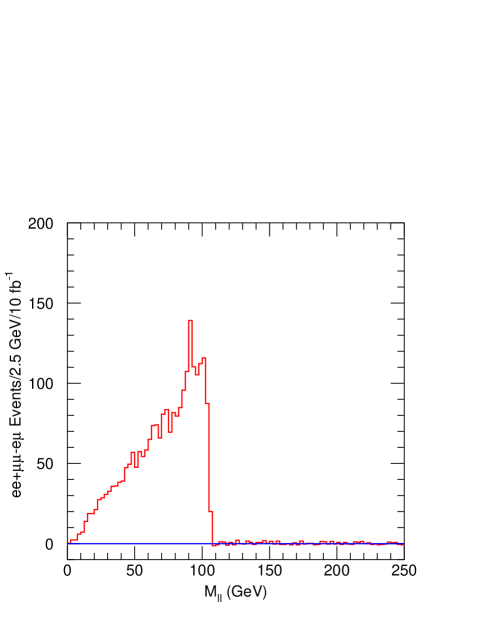
Figure 1: $M_{\ell\ell}$ distribution for $e^{+}e^{-}+\mu^{+}\mu^{-}-e^{\pm}\mu^{\mp}$ events with two photons and two isolated leptons arising at Point G1a. The Standard Model background is negligible.

From the same sample of events with two leptons and two photons, the smaller of the two $\ell^{+}\ell^{-}\gamma$ masses is formed and the resulting mass distribution is shown in Figure 2. The endpoint is at

$$\sqrt{M_{\tilde{\chi}_{2}^{0}}^{2}-M_{\chi_{1}^{0}}^{2}}=189.7\,{\rm GeV}\,,$$

the kinematic limit for $\tilde{\chi}_{2}^{0}\to{\tilde{G}}\ell^{+}\ell^{-}\gamma$. Instead of having a sharp edge like Figure 1, this distribution vanishes linearly because of four-body phase space. The figure shows as a dotted line a linear fit to the end of the spectrum. From this fit the precise end point can be determined. The smaller statistical sample and the need for a fit imply that the resulting uncertainty on the value of the end point is larger. We estimate the precision from Figure 2 to be $\pm 500$ MeV; the full LHC luminosity of 100 fb^-1 should enable this uncertainty to be reduced to $\pm 200$ MeV.

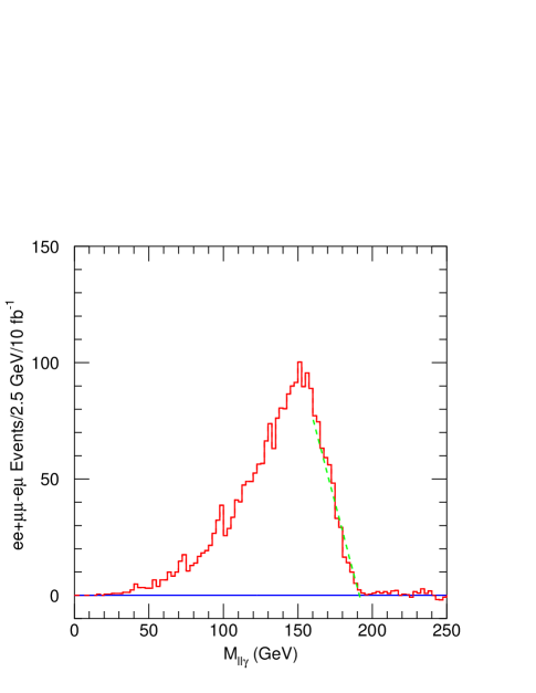
Figure 2: $M_{\ell\ell\gamma}$ distribution for $e^{+}e^{-}+\mu^{+}\mu^{-}-e^{\pm}\mu^{\mp}$ events with two photons at Point G1a. A linear fit from 160 to 190 GeV used to determine the position of the 4-body endpoint is also shown as a dashed line.

The subset of events where one $\ell^{+}\ell^{-}\gamma$ mass is larger and the other smaller than this endpoint was then selected. Only the combination with the lower $\ell\ell\gamma$ mass can come from $\tilde{\chi}_{2}^{0}$ decay. The $M_{\ell^{\pm}\gamma}$ distribution for this combination is shown in Figure 3. Two structures are present in this plot. There is a sharp edge at

$$\sqrt{M_{\tilde{\ell}_{R}}^{2}-M_{\chi_{1}^{0}}^{2}}=112.7\,{\rm GeV}$$

from the photon and the second (“right”) lepton in the decay chain ($\tilde{\ell}\to\ell\gamma$), and there is a distribution that vanishes linearly at

$$\sqrt{M_{\chi_{2}^{0}}^{2}-M_{\tilde{\ell}_{R}}^{2}}=152.6\,{\rm GeV}$$

from the photon and the first (“wrong”) lepton. The former of these has a background from the latter. The plot shows a linear fit between 115 and 150 GeV, which can be used to determine the position of the second endpoint. We estimate the errors on these quantities to be $\pm 200$ and $\pm 500$ MeV for luminosity of 10 fb^-1 where they are limited by statistics. We expect that that they will become limited by systematics at $\pm 100$ and $\pm 200$ MeV at LHC design luminosity.

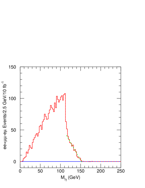
Figure 3: $M_{\ell^{\pm}\gamma}$ distribution for $e^{+}e^{-}+\mu^{+}\mu^{-}-e^{\pm}\mu^{\mp}$ events sample with two photons; a linear fit from 115 to 150 GeV is used to determine the endpoint for the photon and the “wrong” lepton and is shown as a dashed line.

These four measurements are sufficient to determine the masses of the particles ($\tilde{\chi}_{2}^{0}$, ${\tilde{\ell}}_{R}$, and ${\tilde{\chi}_{1}^{0}}$) in this decay chain without assuming any model of SUSY breaking. Of course the existence of, and rate for, this decay chain are model dependent. So is the interpretation of the slepton mass as the mass of the ${\tilde{\ell}}_{R}$. A similar combination of three-body and four-body distributions will be useful in other cases for which a decay chain involving three two-body steps can be identified.

2.2 Reconstruction of ${\tilde{G}}$ Momenta

The supersymmetry events each have two unobserved ${\tilde{G}}$’s. The sum of their transverse momenta is, up to resolution effects and possible missing neutrinos, measured as the two components of $\hbox to0.0pt{\hbox to7.95831pt{\hfil/\hfil}\hss}E_{T}$. There appears to be insufficient information to reconstruct their momenta. However the decay chain

$$\tilde{\chi}_{2}^{0}\to{\tilde{\ell}}^{\pm}\ell^{\mp}\to{\tilde{\chi}_{1}^{0}}\ell^{\pm}\ell^{\mp}\to{\tilde{G}}\gamma\ell^{\pm}\ell^{\mp}\,.$$

provides three precisely measured final state particles and three mass constraints using the masses determined from the measurements in the previous subsection. A $0C$ fit for the ${\tilde{G}}$ momentum is then possible assuming that $M_{{\tilde{G}}}=0$. The solution has a 4-fold ambiguity since the leptons cannot be uniquely assigned and there is quadratic ambiguity from the solution to the constraints. The details are presented in the appendix.

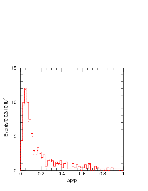
Figure 4: The distribution in $\left|\Delta p\right|/\left|p\right|$ for reconstructed gravitino momenta. The gravitino momenta are reconstructed using the method described in the text. The difference ($\Delta p$) between the reconstructed ($p$) and generated momentum is then formed for the combination with the lowest $\chi^{2}$. Events are included where the lowest $\chi^{2}$ is less than 10 or 1 (dashed line).

We want to have a $\tilde{\chi}_{2}^{0}\to\ell^{+}\ell^{-}\gamma{\tilde{G}}$ decay on both sides of the event. We therefore select events with four leptons and two photons. We require two opposite-sign, same-flavor lepton pairs and a unique way of combining these with the photons consistent with $\tilde{\chi}_{2}^{0}$ decay. Then there are a total of 16 solutions. $\hbox to0.0pt{\hbox to7.95831pt{\hfil/\hfil}\hss}E_{T}$ can be used to resolve these ambiguities as follows. The best solution is selected by summing the momenta of the two ${\tilde{G}}$’s and calculating the $\chi^{2}$ for matching this to the measured value of $\hbox to0.0pt{\hbox to7.95831pt{\hfil/\hfil}\hss}E_{T}$,

$$\chi^{2}=\left({\hbox to0.0pt{\hbox to7.95831pt{\hfil/\hfil}\hss}E_{x}-p_{1x}-p_{2x}\over\Delta\hbox to0.0pt{\hbox to7.95831pt{\hfil/\hfil}\hss}E_{x}}\right)^{2}+\left({\hbox to0.0pt{\hbox to7.95831pt{\hfil/\hfil}\hss}E_{y}-p_{1y}-p_{2y}\over\Delta\hbox to0.0pt{\hbox to7.95831pt{\hfil/\hfil}\hss}E_{y}}\right)^{2}\,.$$

We then select the solution that has the lowest $\chi^{2}$ ($\chi^{2}_{\rm min}$). It is assumed that the resolution in $\hbox to0.0pt{\hbox to7.95831pt{\hfil/\hfil}\hss}E_{T}$ is determined by the total transverse energy $E_{T}$,

$$\Delta\hbox to0.0pt{\hbox to7.95831pt{\hfil/\hfil}\hss}E_{x}=\Delta\hbox to0.0pt{\hbox to7.95831pt{\hfil/\hfil}\hss}E_{x}=0.6\sqrt{E_{T}}+0.03E_{T}$$

We can evaluate the effectiveness of this method by comparing the reconstructed values of the ${\tilde{G}}$ momentum to the best match with the generated values. Figure 4 shows the distribution of the fractional difference between the generated and reconstructed $\tilde{G}$ momentum

$${\Delta p\over p}={\left|\vec{p}_{\rm recon}-\vec{p}_{\rm gen}\right|\over\left|\vec{p}_{\rm gen}\right|}$$

for solutions where $\chi^{2}_{\rm min}<10$; the distribution for $\chi^{2}_{\rm min}<1$ is very similar. As can be seen from the figure which indicates a resolution of order 10% with a long tail, showing that the method works quite well. In approximately 40% of the events that enter this analysis, the $\tilde{G}$ momenta reconstructed within 10% of their nominal value. The shape of this distribution is dominated by detector resolution on the leptons and photons. It is much narrower if the generated momenta are used, and it is significantly wider if the resolution for the electron energy is taken from the calorimeter alone; the central tracker is important for soft electrons.

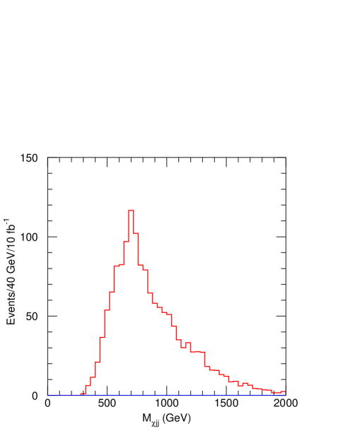
Figure 5: Invariant mass of $\tilde{\chi}_{2}^{0}$ and two jets, for events at Point G1a. The peak is due to the decay $\tilde{g}\to q\overline{q}\tilde{\chi}_{2}^{0}$. Events are required to have two $\tilde{\chi}_{2}^{0}$ momenta reconstructed and at least four jets with $p_{T}>75$ GeV.

2.3 Reconstruction of Gluinos and Squarks

Squark production is significant at Point G1a even though squarks are considerably heavier than gluinos. The reconstruction technique of the previous section can be extended to allow the chain $\tilde{q}\to\tilde{g}q\to\tilde{\chi}_{2}^{0}\overline{q}qq$ to be reconstructed and the gluino and squark masses measured. We begin with the events selected in the previous section where two $\tilde{\chi}_{2}^{0}$ momenta each arising from $\tilde{\chi}_{2}^{0}\to\ell^{+}\ell^{-}\gamma{\tilde{G}}$ have been reconstructed. Jets are are then searched for that have $p_{T}>75\,{\rm GeV}$ in a cone $R=0.4$. We require that at least four such jets be present in the event. Each $\tilde{\chi}_{2}^{0}$ is then combined with two and with three jets; the resulting invariant mass distributions are shown in Figures 5 and 6 respectively. The $jj\tilde{\chi}_{2}^{0}$ mass of Figure 5 has a peak close to the gluino mass, of $744\,{\rm GeV}$, while Figure 6 has a broader peak near the squark masses, $935$–$985\,{\rm GeV}$. The peaks occur in essentially the same place if the jet cut is raised to $p_{T}>100\,{\rm GeV}$ and so are not simply reflections of the kinematic cuts. It is important to emphasize that this technique enables the masses of the squarks and leptons to be measured directly rather than being inferred from features in kinematic distributions.

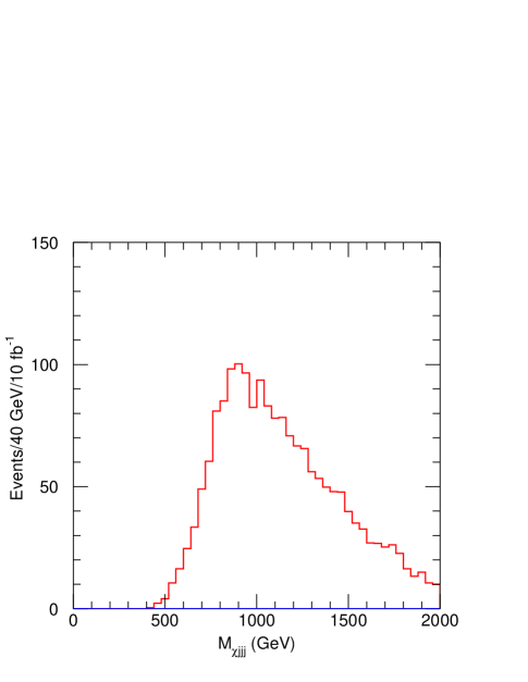
Figure 6: Invariant mass of $\tilde{\chi}_{2}^{0}$ and three jets, for events at Point G1a. The peak is due to the decay $\tilde{q}\to q\tilde{g}\to qq\overline{q}\tilde{\chi}_{2}^{0}$.

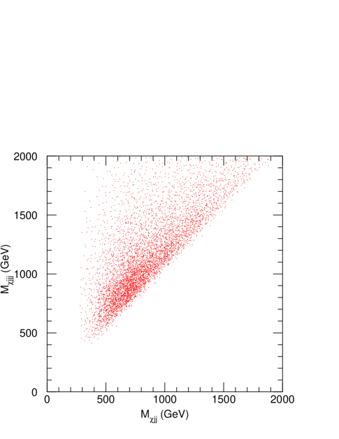
Figure 7: Scatter plot of $M(\tilde{\chi}_{2}^{0}jjj)$ vs. $M(\tilde{\chi}_{2}^{0}jj)$ for events at Point G1a where two $\tilde{\chi}_{2}^{0}$ momenta are reconstructed and there are at least four jets with $p_{T}>75$ GeV.

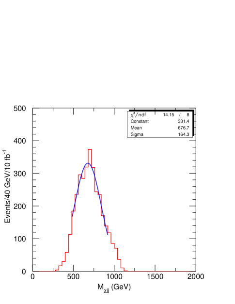
Figure 8: Projection of Figure 7 on the $M(\tilde{\chi}_{2}^{0}jj)$ axis for $800\,{\rm GeV}<M(\tilde{\chi}_{2}^{0}jjj)<1000\,{\rm GeV}$. The peak corresponds to gluino decay. The fit shown is a Gaussian over the range 500 to 900 GeV.

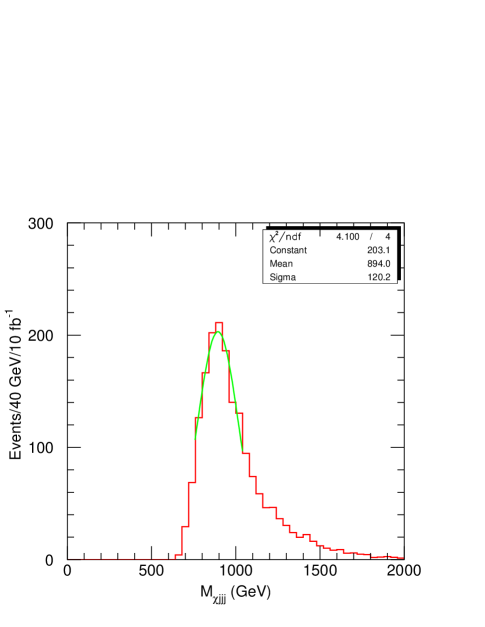
Figure 9: Projection of Figure 7 on the $M(\tilde{\chi}_{2}^{0}jjj)$ axis for $600\,{\rm GeV}<M(\tilde{\chi}_{2}^{0}jj)<800\,{\rm GeV}$. The peak corresponds to squark decay. The fit shown is a Gaussian over the range 760 to 1020 GeV.

The peaks can be sharpened up considerably by searching for correlations since, for each $\tilde{\chi}_{2}^{0}$ momentum and set of three jets, there should be one $\tilde{\chi}_{2}^{0}jjj$ peak at the squark mass mass and three $\tilde{\chi}_{2}^{0}jj$ mass combinations, one of which is at the gluino mass. The scatter plot of all combinations is shown in Figure 7. While the points show significant scatter, there is, nevertheless, a clear peak in the $M(\tilde{\chi}_{2}^{0}jj)$ projection, made by selecting events in the range $800\,{\rm GeV}<M(\tilde{\chi}_{2}^{0}jjj)<1200\,{\rm GeV}$, shown in Figure 8. The smooth curve shown in this plot is a Gaussian fit over the range 500 to 900 GeV; shows a clear maximum at $699\,{\rm GeV}$. If a cut around this peak, $600\,{\rm GeV}<M(\tilde{\chi}_{2}^{0}jj)<800\,{\rm GeV}$, is made a projection of the scatter plot onto the $jjj\tilde{\chi}_{2}^{0}$ axis made as shown in Figure 9, a somewhat narrower peak at the squark mass than that of Figure 6 is obtained. The smooth curve is again a Gaussian fit over the range 760 to 1020 GeV and has a maximum at about $909\,{\rm GeV}$. The statistical errors on the locations of the peaks are quite small and the precision of the measurements is likely dominated by systematic effects such as the calibration of the jet energy scale.

3 Point G1b

In this case the NLSP is neutral and long lived. Almost all of the produced NLSP’s exit the detector without interacting, so the phenomenology is qualitatively similar to the SUGRA models. We first see evidence for new physics via the presence of events with large total $E_{T}$, large $\hbox to0.0pt{\hbox to7.95831pt{\hfil/\hfil}\hss}E_{T}$, and isolated leptons. Approximately 0.1% of the NLSP’s will decay within the detector volume, resulting in a photon that does not point to the interaction vertex. The ability to identify such photons and measure the decay point would provide a valuable constraint on the lifetime and hence information on $C_{\rm grav}$. We anticipate that a decay probability of 0.1% will be difficult but perhaps possible to detect. Apart from this feature, this case is similar to one of the SUGRA cases (Point 4) studied earlier  [1, 3]. In that case, there was more structure in the dilepton spectra as significant production of $\tilde{\chi}_{3}^{0}$ and $\tilde{\chi}_{4}^{0}$ occurs in the decay of a gluino.

3.1 Effective Mass Analysis at Point G1b

Events that have at least four jets are selected and the scalar sum of the $p_{T}$’s of the four hardest jets and the missing transverse energy $\hbox to0.0pt{\hbox to7.95831pt{\hfil/\hfil}\hss}E_{T}$, formed

$$M_{\rm eff}=p_{T,1}+p_{T,2}+p_{T,3}+p_{T,4}+\hbox to0.0pt{\hbox to7.95831pt{\hfil/\hfil}\hss}E_{T}\,.$$

Here the jet $p_{T}$’s have been ordered such that $p_{T,1}$ is the transverse momentum of the leading jet. Figure 10 shows the distribution in $M_{eff}$ for events where the following cuts have been made.

• $\hbox to0.0pt{\hbox to7.95831pt{\hfil/\hfil}\hss}E_{T}>100\,{\rm GeV}$;

• $\geq 4$ jets with $p_{T}>50\,{\rm GeV}$ and $p_{T,1}>100\,{\rm GeV}$;

• Transverse sphericity $S_{T}>0.2$;

• No $\mu$ or isolated $e$ with $p_{T}>20\,{\rm GeV}$ and $|\eta|<2.5$;

• $\hbox to0.0pt{\hbox to7.95831pt{\hfil/\hfil}\hss}E_{T}>0.2M_{\rm eff}$.

It can be seen clearly from this figure that there is an excess of events at large $M_{\rm eff}$ over that expected in the Standard Model, providing clear evidence for new physics.

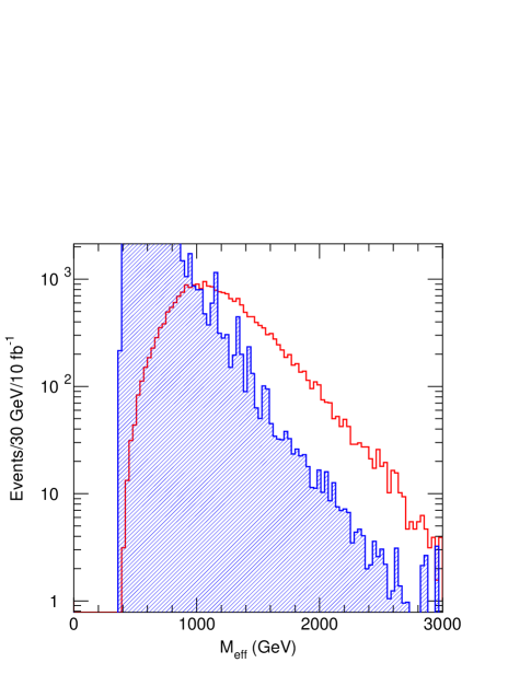
Figure 10: The effective mass distribution showing LHC Point G1b signal and Standard Model backgrounds (hatched histogram)

3.2 Selection of Dilepton events

We attempt to extract the decay chain $\tilde{\chi}_{2}^{0}\to\ell\tilde{\ell}_{R}\to\ell^{+}\ell^{-}{\tilde{\chi}_{1}^{0}}$ as follows. Events are selected that have $M_{\rm eff}>1000$ GeV and $\hbox to0.0pt{\hbox to7.95831pt{\hfil/\hfil}\hss}E_{T}>0.1M_{\rm eff}$, and two and only two isolated leptons of opposite charge with $p_{T}>20$ GeV for electrons, $p_{T}>5$ GeV for muons, and $\left|\eta\right|<2.5$ for both. In order to reduce the combinatorial background we again look at the combination $e^{+}e^{-}+\mu^{+}\mu^{-}-e^{\pm}\mu^{\mp}$. Figure 11 shows the dilepton mass distribution. There is a clear endpoint at

$$M_{e}=M_{\tilde{\chi}_{2}^{0}}\sqrt{1-\left(M_{{\tilde{\ell}}_{R}}\over M_{\tilde{\chi}_{2}^{0}}\right)^{2}}\sqrt{1-\left(M_{{\tilde{\chi}_{1}^{0}}}\over M_{{\tilde{\ell}}_{R}}\right)^{2}}=105.1\,{\rm GeV}.$$

We expect this to have a precision of order 0.1% on the position of this end point. The Standard Model background shown on this plot reflects the poor statistics of our sample, the actual background is much smaller. The figure also shows a small, but statistically significant, peak from $Z$ decays. These are arising from the decay $\chi_{2}^{0}\to\chi_{1}^{0}Z$ which has a branching ratio of 9%. The fact that this two body decay is of the same order of magnitude as the $\ell^{+}\ell^{-}{\tilde{\chi}_{1}^{0}}$ decay is strong evidence that the latter is not arising from the three body decay $\chi_{2}^{0}\to\chi_{1}^{0}\ell^{+}\ell^{-}$ but from the sequence of two 2-body decays. Additional evidence is provided by the shape of the edge. We can be confident therefore that the endpoint is measuring the combination of masses in the above equation.

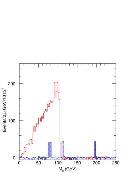
Figure 11: The dilepton mass distribution at Point G1b. The Standard Model background (hatched histogram) is very small. The fluctuations in our event sample for the combination shown ı.e. $e^{+}e^{-}+\mu^{+}\mu^{-}-e^{\pm}\mu^{\mp}$ are therefore larger than one would expect in 10 fb^-1.

3.3 Extraction of gluino

We now select events from the previous sample that have at least two jets with $p_{T}>125$ GeV and require that the dilepton mass is below 105 GeV. The invariant mass of the $\ell^{+}\ell^{-}jj$ system is shown in Figure 12 where again to reduce combinatorial background we look at the combination $e^{+}e^{-}+\mu^{+}\mu^{-}-e^{\pm}\mu^{\mp}$. All combinations of jets with $p_{T}>25$ GeV are shown. The figure shows a broad peak but no clear structure. The events in this plot are dominated by decay $\tilde{g}\to q\overline{q}\tilde{\chi}_{2}^{0}\to q\overline{q}\ell^{+}\ell^{-}{\tilde{\chi}_{1}^{0}}$. However the large combinatorial problem prevents a kinematic edge from being visible. In order to estimate the sensitivity to the gluino mass, we generate another set of events which differ only in that the gluino mass has been increased to 800 GeV. The distribution from this sample is shown as the dashed histogram in Figure 12. The total event rate for this sample has been increased by a factor of 1.24, to compensate for the smaller production rate and to facilitate a comparison of shapes of the distributions. It is clear from this figure that these two curves could be distinguished and that a constraint on the gluino mass obtained. The different event rates is not directly usable as a mass constraint as the branching ratios are not known.

The signal can be improved somewhat if we restrict the jets to be those that arise from bottom quark jets. The resulting distribution is shown in Figure 13 which is identical to that for Figure 12 except that the jets are required to be tagged as b-jets. The mass distribution has a clear structure which reflects the kinematic end point of the dijet-dilepton system at

$$\mathopen{{missing\hbox{$\left missing\vbox to0.0pt{}\right.\n@space$}}}[{50pt}(M_{\tilde{g}}-M_{\chi_{2}^{0}})^{2}+M_{e}^{2}$$

$$\quad+\frac{M_{\tilde{g}}-M_{\tilde{\chi}_{2}^{0}}}{2M_{\tilde{\chi}_{2}^{0}}}\mathopen{{missing\hbox{$\left missing\vbox to0.0pt{}\right.\n@space$}}}({48pt}M_{\tilde{\tilde{\chi}_{2}^{0}}}^{2}-M_{\tilde{\ell}}^{2}+\frac{(M_{\tilde{\chi}_{2}^{0}}^{2}+M_{\ell}^{2})(M_{\ell}^{2}-M_{\tilde{\chi}_{1}^{0}}^{2})}{2M_{\ell}^{2}}\left(1+\frac{M_{\tilde{\chi}_{2}^{0}}^{2}-M_{\ell}^{2}}{2M_{\tilde{\chi}_{2}^{0}}M_{\ell}}\right)\mathclose{{missing\hbox{$\left missing\vbox to0.0pt{}\right.\n@space$}}}){48pt}\mathclose{{missing\hbox{$\left missing\vbox to0.0pt{}\right.\n@space$}}}]{50pt}^{1/2}$$

$M_{e}$ is the value of the dilepton edge defined above (the b quark mass is neglected in this result). This dilepton-dijet endpoint corresponds to 629 GeV. The dashed line on the figure shows the result when the gluino mass is increased to 800 GeV; the kinematic end point is now at 673 GeV. The event rates in this plot are rather low and to obtain precision using this method 100 fb^-1 of integrated luminosity will be needed.

Following in the spirit of Ref. , we attempt to look for kinematic structure in the dijet mass distribution from the decay $\tilde{g}\to q\overline{q}\tilde{\chi}_{2}^{0}\to q\overline{q}\ell^{+}\ell^{-}{\tilde{\chi}_{1}^{0}}$. We begin by selecting events with $M_{\rm eff}>1000$ GeV and $\hbox to0.0pt{\hbox to7.95831pt{\hfil/\hfil}\hss}E_{T}>0.1M_{\rm eff}$ and four isolated leptons. We retain the event if these lepton can be grouped into two opposite-sign, same flavor pairs each of which has an invariant mass below 105 GeV. We then select the four jets with the highest transverse momenta, and pair them up, selecting the combination that gives the smallest value for the sum of the two pair masses. A plot of the mass distribution of a dilepton pair and one of the jet pairs is similar, with poorer statistics, to that of Figure 12; there is still no clear kinematic feature. Figure 14 shows the invariant mass of each of the jet pairs(two entries per event). The end-point that one expects to see at $m_{\tilde{g}}-m_{\tilde{\chi}_{2}^{0}}$ is not visible. However the shape of this curve is sensitive to the gluino mass as can be seen by comparing the dashed histogram which is the result of the same event selection applied to an event sample where the gluino mass is raised to 800 GeV. A detailed study  [3] of a case similar to this concluded that one could measure the mass difference $m_{\tilde{g}}-m_{\tilde{\chi}_{2}^{0}}$ with an uncertainty of order 3% with an event sample approximately 10 times larger than this one (the cross-section is approximately 3 times larger due to the smaller gluino mass of 580 GeV and 30 fb^-1 of data was assumed). We will conservatively assume that we can determine $m_{\tilde{g}}-m_{\tilde{\chi}_{2}^{0}}$ with an uncertainty of 50 GeV, i.e. the difference shown in the figures.

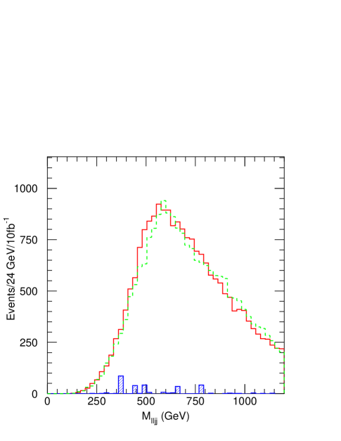
Figure 12: The mass distribution of a dilepton and two jets at Point  G1b. The dotted histogram corresponds to a different event sample where the gluino mass is changed to 800 GeV, this distribution has been scaled by a factor of 1.24 to facilitate comparison of the shapes. The Standard Model background is shown as the hatched histogram.

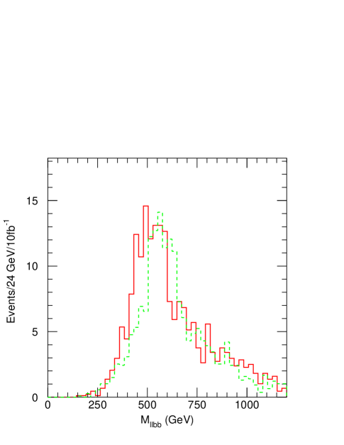
Figure 13: The mass distribution of a dilepton and two b-jets at Point  G1b. The dashed histogram corresponds to a different event sample where the gluino mass is changed to 800 GeV. No standard model background events passed the cuts.

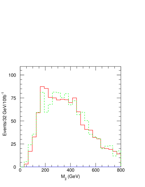
Figure 14: The mass distribution of two jets at Point  G1b. There are two entries per event. The dotted histogram corresponds to a different event sample where the gluino mass is changed to 800 GeV, this distribution has been scaled by a factor of 1.18 to facilitate comparison of the shapes. No Standard Model events passed the cuts.

3.4 Extraction of squarks

In view of the lack of clear structure in the events of the previous section, it will be very difficult to extract the cascade decay $\tilde{q}\to\tilde{g}q\to q\overline{q}q\tilde{\chi}_{2}$ as was possible in the case of G1a. We therefore attempt to extract the decay $\tilde{q}\to q\tilde{W}\to qW{\tilde{\chi}_{1}^{0}}$. We first select events with $M_{\rm eff}>1000$ GeV and $\hbox to0.0pt{\hbox to7.95831pt{\hfil/\hfil}\hss}E_{T}>0.1M_{\rm eff}$ and only two isolated leptons which can form any of the following combinations: $e^{+}e^{+}$, $e^{-}e^{-}$, $\mu^{+}\mu^{+}$, $\mu^{-}\mu^{-}$ or $e\mu$ (any charges). In addition we require that there be two jets each with $p_{T}>450$ GeV. Few events pass this selection, but in those that do 60% of the directly produced supersymmetric particles are squarks. Figure 15 shows the lepton jet invariant mass distribution. In order to assess the sensitivity of this distribution to the squark mass, another event sample was produced where the squark masses were reduced by 50 GeV. The distribution from this sample is shown as the dashed histogram in Figure 15. The shapes are significantly different; the shifting to the left of the dashed histogram is symptomatic of the smaller mass of the squark. A Kolmogorov test applied to the shape of the histograms in Figure 15 using finer binning and data samples corresponding to 30 fb^-1 of integrated luminosity indicates that they are distinct with a probability of 92%. Sensitivity to squark masses at the 50 GeV level should therefore be possible.

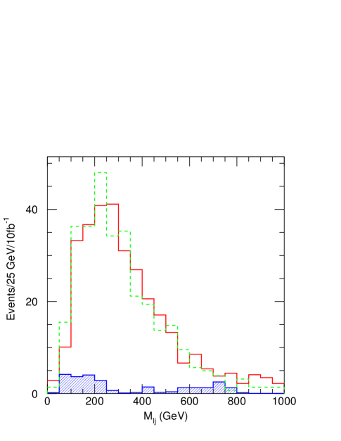
Figure 15: The mass distribution of a lepton+ jet system. The dashed histogram corresponds to a different event sample where the squark mass has been reduced by 50 GeV. The Standard Model background shown as a hatched histogram is dominated by $t\overline{t}$ production.

4 Point G2a

The total supersymmetry supersymmetry cross-section for both cases G2a and G2b is 23 pb, larger than that of cases G1 because the squark masses are considerably lower. Since the slepton is the NLSP, almost all supersymmetry events contain a pair of sleptons. Most of these sleptons are produced in the decays $\tilde{\chi}_{2}^{0}\to\ell\tilde{\ell}$ and $\tilde{\chi}_{1}^{0}\to\ell\tilde{\ell}$. In the case of Point G2a, the NLSP decays with a very short decay length (52 $\mu$) to give an additional lepton. If the produced sleptons are selectrons or smuons, the high multiplicity of produced isolated leptons will provide both a convenient trigger and the first evidence for new physics. Only in the case where both sleptons are staus and decay hadronically, will we have to rely upon a jet and missing-$E_{T}$ trigger for the first indication of new physics.

4.1 Dilepton Distributions

As the branching ratios for $\tilde{\chi}_{i}^{0}\to\tilde{\ell}_{R}\to\tilde{G}\ell^{+}\ell^{-}$ are substantial we can attempt to select this decay chain by searching for events with isolated leptons and jets as most of the $\tilde{\chi}_{i}^{0}$ will be produced in the decay of strongly interacting sparticles. Events are selected that have at least 4 jets with $p_{T}>25$ GeV and $\left|\eta\right|<2.5$ and at least 4 charged tracks associated with each jet (to eliminate jets from hadronic tau decays). An $M_{\rm eff}$ is formed from the scalar sum of the transverse energies of the four jets with the largest $p_{T}$ and $\hbox to0.0pt{\hbox to7.95831pt{\hfil/\hfil}\hss}E_{T}$.

$$M_{\rm eff}=p_{T,1}+p_{T,2}+p_{T,3}+p_{T,4}+\hbox to0.0pt{\hbox to7.95831pt{\hfil/\hfil}\hss}E_{T}\,.$$

We then require $M_{\rm eff}>400$ GeV and $\hbox to0.0pt{\hbox to7.95831pt{\hfil/\hfil}\hss}E_{T}>0.2M_{\rm eff}$.

An additional selection requiring two oppositely charged leptons (either electrons or muons) with $p_{T}>10$ GeV and $\left|\eta\right|<2.5$ is made and the dilepton mass distribution formed. In order to reduce combinatoric background, we form the combination $e^{+}e^{-}+\mu^{+}\mu^{-}-e^{\pm}\mu^{\mp}$. The mass distribution for this combination is shown in Figure 16. Two edges are visible at 52 and 175 GeV. corresponding to

$$\sqrt{M_{\tilde{\chi}_{1}^{0}}^{2}-M_{{\tilde{\ell}}_{R}}^{2}}=52.1\,{\rm GeV}$$

and

$$\sqrt{M_{\tilde{\chi}_{2}^{0}}^{2}-M_{{\tilde{\ell}}_{R}}^{2}}=175.9\,{\rm GeV}\,.$$

The Standard Model background shown on this plot appears not to be negligible. However this is somewhat misleading as our background sample does not correspond to the statistical fluctuations expected for an integrated luminosity of 10 fb^-1. The number of background events can be seen more clearly in Figure 17 which shows the combination $e^{+}e^{-}+\mu^{+}\mu^{-}+e^{\pm}\mu^{\mp}$. It can be seen from this figure that this combination has considerable combinatorial background in the signal events; the edge at 175 GeV is less clear. From this plot one can estimate that, in the mass range 60 to 170 GeV, the true Standard Model background in Figure 16 is $0\pm 60$; this fluctuation is insignificant compared with the $\sim 4000$ signal events in the same region.

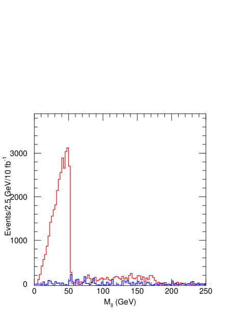
Figure 16: $M_{\ell\ell}$ distribution for the flavor subtracted combination $e^{+}e^{-}+\mu^{+}\mu^{-}-e^{\pm}\mu^{\mp}$ of events having two isolated leptons arising at Point G2a. The Standard Model background shown does not represent the statistical fluctuations expected in 10 fb^-1 of integrated luminosity (see text).

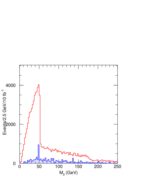
Figure 17: $M_{\ell\ell}$ distribution for all oppositely charged dilepton pairs $e^{+}e^{-}+\mu^{+}\mu^{-}+e^{\pm}\mu^{\mp}$ in events having two isolated leptons arising at Point G2a. The background, mostly from $t\overline{t}$ production, is shown as the hatched histogram.

It is clear that the statistical error on the precision the measurement of the position of the lower edge will be small and the systematic errors will dominate. The higher edge has much poorer statistics, so we have used a fit to estimate how well the endpoint might be measured. Before any cuts, the signal distribution in $M_{\ell\ell}$ has the form

$$\frac{dN}{dM_{\ell\ell}}=A(1+M_{\ell\ell})\theta(M_{\rm max}-M_{\ell\ell})$$

where $M_{\rm max}$ is the position of the edge. We add to this a background $B$ taken to be constant in the vicinity of the edge and then smear with a Gaussian of width $\sigma_{M}$ to be determined by the fit. We then use the PAW version of MINUIT [16] to fit the data set of Figure 16, whose statistical fluctuations represent approximately $10$ fb^-1 of integrated luminosity, over the ranges $20\,{\rm GeV}<M_{\ell\ell}<80\,{\rm GeV}$ and $150\,{\rm GeV}<M_{\ell\ell}<250\,{\rm GeV}$. The best fits are shown in Figure 18, and the fits give

$M_{\rm max}=52.266^{+0.058}_{-0.045}$ GeV	$\sigma_{M}=0.86$ GeV
$M_{\rm max}=175.46^{+0.21}_{-0.22}$ GeV	$\sigma_{M}=6.5$ GeV

The errors on $M_{\rm max}$ are determined by MINOS [16]. We can expect systematic uncertainties of order $0.1\%$ on these measurements. We therefore expect that the precision of the upper edge will be limited by statistics even for 100 fb^-1 of data. For the purposes of parameter fitting below, we will assume that the errors are 70 and 270 MeV for 10 fb^-1 and 50 and 180 MeV for 100 fb^-1 respectively.

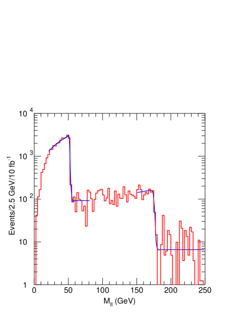
Figure 18: As Figure 16 except that the distribution is shown on a logarithmic scale and the fits to the edges described in the text are shown. No background is shown on this figure.

4.2 Detection of $\tilde{q}_{R}$

Here we use the decay chain $\tilde{q}_{R}\to q\tilde{\chi}_{1}^{0}\to q{\tilde{\ell}}_{R}^{\pm}\ell^{\mp}\to q\tilde{G}\ell^{+}\ell^{-}$. The same event selection as in Section 4.1 is used with the addition of the requirement that the dilepton pair have mass $M_{\ell\ell}<52$ GeV and transverse momentum $p_{T}(\ell\ell)>75$ GeV to enhance the probability that the leptons come from the same decay chain. The two jets with the largest transverse momentum were then selected; each is required to have $p_{T}>50\,{\rm GeV}$ and and to contain least 4 charged tracks. We show the invariant mass of the dilepton and one of these two jets ($\ell^{+}\ell^{-}j$) in Figure 19 and of one the leptons and a jet in ($\ell^{\pm}j$) distributions are show in Figure 20. In each case only the smaller of the various mass combinations is plotted and again we shown the subtracted distributions $e^{+}e^{-}+\mu^{+}\mu^{-}-e^{\pm}\mu^{\mp}$ which have a cleaner structure.

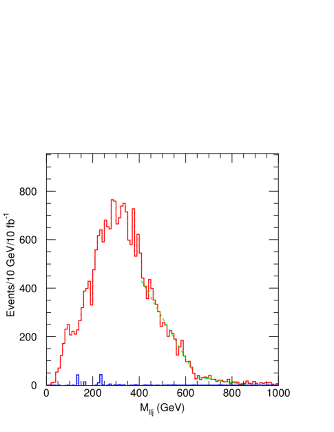
Figure 19: $M_{\ell\ell j}$ mass spectrum at Point G2a for events that contain at least two isolated leptons and four jets. The linear fit shown as a dashed line is over the range 390 to 590 GeV. The Standard Model background is shown as the hatched histogram.

The $\ell^{+}\ell^{-}q$ distribution has an expected endpoint at

$$M_{\ell\ell q}^{\rm max}=\sqrt{M_{\tilde{q}_{R}}^{2}-M_{{\tilde{\ell}}_{R}}^{2}}=640.12\,{\rm GeV}$$

while the $\ell^{\pm}q$ distribution has an expected endpoint at

$$M_{\ell q}^{\rm max}=\sqrt{M_{\tilde{q}_{R}}^{2}-M_{{\tilde{\chi}_{1}^{0}}}^{2}}\sqrt{1-{M_{{\tilde{\ell}}_{R}}^{2}\over M_{{\tilde{\chi}_{1}^{0}}}^{2}}}=289.16\,{\rm GeV}\,.$$

The plots show a linear fit below the end points. These fits extrapolate to end points slightly larger than the actual values. The errors on the precision of these values will be dominated by the systematic uncertainties in the jet energy scales estimated to be of order 1%. We expect that the systematic uncertainty in the measurement of the ratio of these two end-points will be less than this.

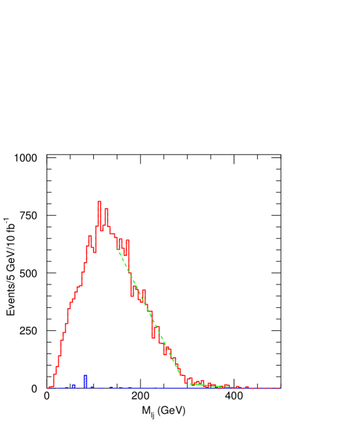
Figure 20: $M_{\ell j}$ mass spectrum at Point G2a. The fits shown as dashed lines correspond to two separate linear fits over the ranges is over the ranges 150 to 280 GeV and 305 to 400 GeV. The former extrapolates to an endpoint at 315 GeV. The Standard Model background is shown as the hatched histogram.

We can now solve for the ${\tilde{\ell}}_{R}$, ${\tilde{\chi}_{1}^{0}}$, and $\tilde{q}_{R}$ masses in terms of the measured endpoints:

$$M_{{\tilde{\ell}}_{R}} = {M_{\ell\ell}\sqrt{M_{\ell\ell q}^{2}-M_{\ell q}^{2}-M_{\ell\ell}^{2}}\over M_{\ell q}}$$

$$M_{{\tilde{\chi}_{1}^{0}}} = \sqrt{M_{\ell\ell}^{2}+M_{{\tilde{\ell}}_{R}}^{2}}$$

$$M_{\tilde{q}_{R}} = \sqrt{M_{\ell\ell q}^{2}+M_{{\tilde{\ell}}_{R}}^{2}}$$

Note that this method for extracting masses requires only the existence of the decay chain; the underlying model is not used in the analysis. Of course the interpretation of the masses as those of $\tilde{q}_{R}$, ${\tilde{\ell}}_{R}$, etc., is model dependent.

4.3 Detection of $\tilde{\chi}_{1}^{\pm}$ decays

Approximately 50% of the decays of $\tilde{q}_{L}$ occur to a $\tilde{\chi}_{1}^{\pm}$. There is a decay chain starting from $\tilde{\chi}_{1}^{\pm}$ proceeding through a slepton and a ${\tilde{\chi}_{1}^{0}}$ that gives a final state with three isolated leptons viz.

$$\tilde{\chi}_{1}^{+}\to\ell^{+}\tilde{\nu}\to{\tilde{\chi}_{1}^{0}}\nu\ell^{+}\to\nu\ell^{+}\ell^{-}\tilde{\ell}_{R}^{+}\to\nu\ell^{+}\ell^{-}\ell^{+}\tilde{G}.$$

The combined branching ratio is 29%. We begin with the event selection of the previous section, requiring that there be at least three isolated leptons in addition to the jets. Events are then required to have at least one opposite sign, same flavor pair with an invariant mass in the range $40$ GeV $<M_{\ell\ell}<$ 52 GeV so that they are likely to have come from a ${\tilde{\chi}_{1}^{0}}$ decay. Any other pairs of leptons of same flavor and opposite sign with $M_{\ell\ell}<$ 175 GeV are discarded as they are likely to come from $\tilde{\chi}_{2}^{0}$ decay. The selected dilepton is then combined with any other remaining lepton and the invariant mass of the trio is shown in Figure 21. If all three selected leptons arose from the decay of $\tilde{\chi}_{1}^{\pm}$, this distribution would have a linear vanishing at

$$\sqrt{M_{\tilde{\chi}_{1}^{\pm}}^{2}-M_{\tilde{\nu}}^{2}+M_{{\tilde{\chi}_{1}^{0}}}^{2}-M_{\tilde{\ell}_{R}}^{2}}=85.75\hbox{ GeV}$$

There is considerable background in this plot. Nevertheless there is clear evidence of structure. While it may not prove possible to extract a precision measurement from this distribution, it provides evidence for the existence of $\tilde{\chi}_{1}^{\pm}$ and a strong consistency check of the model.

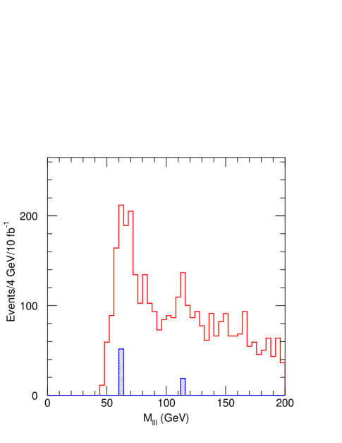
Figure 21: $M_{\ell\ell\ell}$ mass spectrum at Point G2a. The Standard Model background (hatched histogram) is very small.

5 Point G2b

In this case the NLSP is the ${\tilde{\tau}}_{1}$, and it has a long lifetime, $c\tau\approx 1\,{\rm km}$. The decay ${\tilde{\ell}}\to{\tilde{\tau}}_{1}\tau\ell$ is not kinematically allowed, so the $\tilde{e}_{R}$ and $\tilde{\mu}_{R}$ are also long-lived. Each event will contain two of these quasi-stable particles which will appear in the detector as a pair of slow muons. These will provide a trigger as the mean velocity is quite large (see below) and the first evidence for new physics in this case.

A small fraction of the sleptons will decay within the detector; significant energy is released in the decay so the result is a track which ends somewhere and a decay product that points back to this end point. If the sparticle in question is a selectron, the resulting electron could be pointed back using the electromagnetic calorimeter in combination with information from the central tracker. If the sparticle is a smuon, the resulting muon would have to be pointed using the remainder of the tracking volume and the outer muon system. If it is a stau, the resulting hadronic decay of the tau might be pointed using a combination of the central tracker and the electromagnetic calorimeter. It is worth emphasizing the importance of measuring this decay length: it is the only way to obtain information on the gravitino couplings and the fundamental scale of supersymmetry breaking.

5.1 Effective mass analysis at Point G2b

The events can be triggered using the quasi-stable particles that will appear as muons. The velocity distribution of these particles is shown in Figure 22, from which it can be seen that the mean velocity is greater than $0.9c$. Hence many of these should pass the ATLAS level-1 muon trigger [17].

The events also have a large amount of missing $E_{T}$ as measured by the calorimeter. The distribution is shown in Figure 23, which has a mean value of $315\,{\rm GeV}$. If the measured momenta of the sleptons is included, the missing energy is much smaller as can be seen from the dotted curve in Figure 23. The true missing $E_{T}$ is larger than standard model backgrounds due to the larger number of taus and heavy flavors in the SUSY sample. The Standard Model background shown on this plot is controlled by the requirement that it contain at least two muons. This calorimetric missing $E_{T}$ could also be used as a trigger.

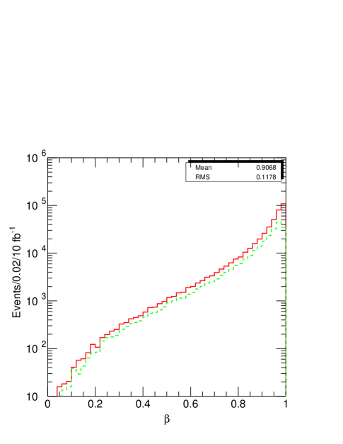
Figure 22: Generated slepton velocity distribution $\beta$ at Point G2b. The dotted curve is for sleptons with $\eta<1$.

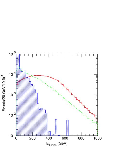
Figure 23: Calorimetric missing transverse energy $\hbox to0.0pt{\hbox to7.95831pt{\hfil/\hfil}\hss}E_{T}$ at Point G2b. The dotted curve shows the true $\hbox to0.0pt{\hbox to7.95831pt{\hfil/\hfil}\hss}E_{T}$ including sleptons. The Standard Model background of dimuon events is shown as the hatched histogram.

We begin the analysis by using the effective mass distribution found by selecting events that have at least four jets and forming scalar sum of the $p_{T}$’s of the four hardest jets and the missing transverse energy $\hbox to0.0pt{\hbox to7.95831pt{\hfil/\hfil}\hss}E_{T}$,

$$M_{\rm eff}=p_{T,1}+p_{T,2}+p_{T,3}+p_{T,4}+\hbox to0.0pt{\hbox to7.95831pt{\hfil/\hfil}\hss}E_{T}\,.$$

Here the jet $p_{T}$’s have been ordered such that $p_{T,1}$ is the transverse momentum of the leading jet. There is no requirement that the jets or missing $E_{T}$ be large enough to provide a trigger; we assume that the events are triggered by the muon system. Note that the Standard Model background shown on this plot is required to have two muons in it and is suppressed as a result. The NLSP’s are ignored when making this effective mass variable. The distribution shown in Figure 24, has a mean value of $1004\,{\rm GeV}$ characteristic of the masses of the strongly interacting sparticles which dominate the production.

There is a peak in the effective mass distribution at zero, corresponding to the production of events which have little hadronic activity and $\hbox to0.0pt{\hbox to7.95831pt{\hfil/\hfil}\hss}E_{T}$. It is due to the direct production of NSLP via such processes as $q\overline{q}\to\tilde{\ell}^{+}\tilde{\ell}^{-}$ and the direct production of $\tilde{\chi}_{1}^{0}$ and $\tilde{\chi}_{1}^{+}$ which then decay to the NLSP. This is shown in Figure 25 which shows the ID codes for the produced primary sparticles and demonstrates that they are mainly sleptons and gauginos. We will discuss these events in more detail below.

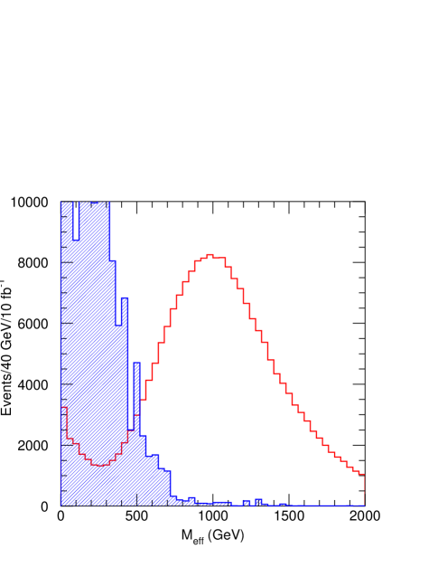
Figure 24: Effective mass distribution not including sleptons at Point G2b. The Standard Model background of dimuon events is shown as the hatched histogram.

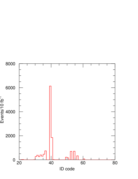
Figure 25: The particle ID codes for the primary particles of events in Figure 24 which have $M_{\rm eff}<100$ GeV: left sleptons (31-36), gauginos (30, 39 and 40) and right sleptons (52, 54, and 56).

5.2 Slepton mass determination

The sleptons (NLSP) are dominantly produced at the end of decay chains and consequently the majority of them are fast. The velocity distribution is shown in Figure 22 from which the mean velocity can be determined. Time of flight measurements in the muon detector system can be used to determine this velocity. When this is combined with a measurement of momentum in the same system, the mass can be obtained.

The muon chambers in the ATLAS detector can provide a time-of-flight resolution of about $1\,{\rm ns}$. For each slepton with $\left|\eta\right|<2.5$ the time delay relative to $\beta=1$ to the outer layer of the muon system, taken to be a cylinder with a radius of $10\,{\rm m}$ and a half-length of $20\,{\rm m}$, is calculated using the generated momentum and smeared with a Gaussian $1\,{\rm ns}$ resolution. The smeared time delay $\Delta t$ and measured momentum are then use to calculate a mass. The resulting mass distribution is shown in Figure 26 for sleptons with $10\,{\rm ns}<\Delta t<50\,{\rm ns}$. Raising the lower limit on $\Delta t$ improves the mass resolution but reduces the efficiency. The resolution is never good enough to resolve the ${\tilde{\tau}}_{1}$ and $\ell_{R}$ masses of $101.35\,{\rm GeV}$ and $102.67\,{\rm GeV}$. The upper limit on $\Delta t$ is somewhat arbitrary; it reflects practical concerns and also eliminates sleptons with very low $\beta$ that lose most of their energy in the calorimeter. The average of the generated distribution, $102.2\,{\rm GeV}$, agrees well with the fitted mean value in Figure 26. It is important to note that this method will provide an mass measurement of an average over the ${\tilde{\tau}}_{1}$, $\tilde{\mu}_{R}$ and $\tilde{e}_{R}$ masses as this analysis cannot distinguish slepton flavors.

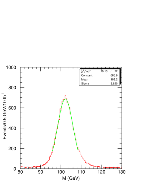
Figure 26: Reconstructed slepton masses for time delays $10\,{\rm ns}<\Delta t<50\,{\rm ns}$ relative to a $\beta=1$ particle.

5.3 Reconstruction of $\tilde{\chi}_{1}^{0}$, $\tilde{\chi}_{2}^{0}$ and $\tilde{\chi}_{4}^{0}$

Since the ${\tilde{\ell}}_{R}$ are quasi-stable, the decays $\tilde{\chi}_{i}^{0}\to{\tilde{\ell}}_{R}\ell$ can be fully reconstructed. Events are selected that have at least three isolated electrons, muons or quasi-stable sleptons with $\left|\eta\right|<2.5$ and $p_{T}>10$ GeV. The two highest $p_{T}$ particles among the sleptons and muons (i.e. those particles that penetrate to the muon system) are assumed to be sleptons and are assigned their measured $\vec{p}$ and the slepton mass; the rest are assumed to be muons. The Standard Model background is already negligible, so there is no need to make a time-of-flight cut to identify the sleptons. Sleptons are then combined with electrons or muons ($\ell$) of the opposite charge and the resulting mass for all ${\tilde{\ell}}^{\pm}\ell^{\mp}$ combinations is plotted in Figure 27; we have no way of determining the flavor of a slepton. There are two narrow peaks at the ${\tilde{\chi}_{1}^{0}}$ and $\tilde{\chi}_{2}^{0}$ masses. The rather strange shape of the ${\tilde{\chi}_{1}^{0}}$ peak is a consequence of the fact that the splitting between the ${\tilde{\chi}_{1}^{0}}$ and ${\tilde{\ell}}_{R}$ is small, so the mass is dominated by the rest mass of the ${\tilde{\ell}}_{R}$. There is a small peak at 348 GeV due to the decay of $\tilde{\chi}_{4}$.

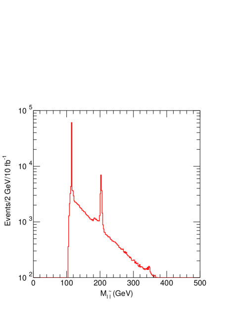
Figure 27: ${\tilde{\ell}}^{\pm}\ell^{\mp}$ mass distribution at Point G2b.

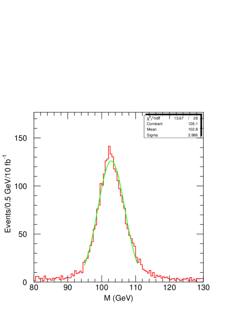
Figure 28: Same as Figure 26 for events in a $\pm 5$ GeV window around the ${\tilde{\chi}_{1}^{0}}$ mass peak of Figure 27 and the lepton is identified as an electron.

The mass measurement of the slepton itself can now be refined and the smuon and selectron separated by using the events in the in the ${\tilde{\chi}_{1}^{0}}$ mass peak. By restricting the event samples to the cases where the lepton is either an electron or muon, this method can be used to provide separate samples of $\tilde{e}_{R}$ and $\tilde{\mu}_{R}$. The analysis of the previous section is now repeated for the events within $\pm 5\,{\rm GeV}$ of the ${\tilde{\chi}_{1}^{0}}$ peak where the lepton is an electron. The resulting distribution, shown in Figure 28 has a mean quite close to the correct $\tilde{e}_{R}$ mass. The statistical error on the mass in from a data sample of 10 fb^-1 is $\sim 100$ MeV. Therefore it should be possible to distinguish the average slepton mass as determined in the previous section from the $\tilde{e}_{R}$ and $\tilde{\mu}_{R}$ masses. The actual errors are likely to be dominated by systematic effects estimate to be 0.1%. This will be sufficient to constrain the mass of the stau which is present in the average from the separate selectron and smuon masses.

5.4 Extraction of $\tilde{\ell}_{L}$

We can begin with the reconstructed ${\tilde{\chi}_{1}^{0}}$ and combine it with another charged lepton in an attempt to detect the decay chain $\tilde{\ell}_{L}\to{\tilde{\chi}_{1}^{0}}\ell\to\tilde{\ell}_{R}^{\pm}\ell^{\mp}\ell$. We select events that have at least two muons or stable sleptons with $p_{T}>10$ GeV and $\left|\eta\right|<2.5$ The two highest $p_{T}$ objects are assigned to be sleptons and the rest are called muons. Combinations of a slepton and either muon or electron are formed that have no net charge and the system is tagged as ${\tilde{\chi}_{1}^{0}}$ if $M_{\ell^{\pm}\ell^{\mp}}=M_{{\tilde{\chi}_{1}^{0}}}\pm 5$ GeV. This ${\tilde{\chi}_{1}^{0}}$ candidate is then combined with another charged lepton and the mass of the three lepton system is shown in Figure 29. There is a clear peak at the slepton mass of 203 GeV.

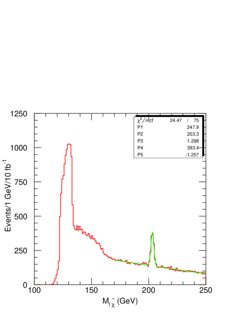
Figure 29: The mass distribution of a slepton and a pair of leptons at Point G2b. Events are selected so that a lepton and a slepton reconstruct to the ${\tilde{\chi}_{1}^{0}}$ mass ($M_{\tilde{\chi}_{1}^{0}}\pm 5$ GeV).

Another feature is also present in this plot. The decay chain $\tilde{\chi}_{1}^{\pm}\to\tilde{\nu}\ell\to{\tilde{\chi}_{1}^{0}}\nu\ell\to\tilde{\ell}_{R}^{\pm}\ell^{\mp}\nu\ell$ has a kinematic upper bound for the mass of the $\tilde{\ell}_{R}^{\pm}\ell^{\mp}\ell$ system of

$$\sqrt{M_{\tilde{\chi}_{1}^{\pm}}^{2}-M_{\tilde{\nu}}^{2}+M_{{\tilde{\chi}_{1}^{0}}}^{2}}=134\hbox{ GeV}$$

The structure below this end-point is clearly visible in Figure 29. However there is a large background so a very accurate measurement will be difficult. Nevertheless, this structure measures a combination of $\tilde{\nu}$ and $\tilde{\chi}_{1}^{\pm}$ and will provide a powerful constraint on the model.

5.5 Reconstruction of Squarks

At this point squarks are considerably lighter than gluinos, reflecting the fact that $m_{\tilde{g}}/m_{\tilde{q}}\sim\sqrt{N_{5}}$ and $N_{5}>1$, as is usually the case when the NLSP is a slepton. Direct production of squarks is dominant and the decay $\tilde{q}_{R}\to\tilde{\chi}_{1}^{0}q$ is large. Events are selected that have a $\ell\tilde{\ell}$ mass within 5 GeV of the ${\tilde{\chi}_{1}^{0}}$ peak in Figure 27. This pair is then combined with any of the four highest $p_{T}$ jets in the event. The resulting mass distribution of the jet-${\tilde{\chi}_{1}^{0}}$ system shown in Figure 30 has a relatively narrow peak somewhat below the average $\tilde{q}_{R}$ mass of $648\,{\rm GeV}$. Some shift is expected since the jets are defined using a small cone size, $R=0.4$.

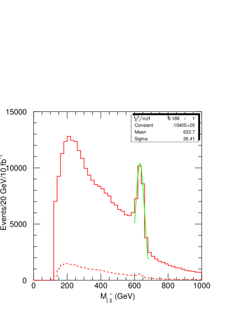
Figure 30: ${\tilde{\chi}_{1}^{0}}$-$q$ mass distribution at Point G2b. Events have a lepton and a slepton with invariant mass in a $\pm 5$ GeV window around the ${\tilde{\chi}_{1}^{0}}$ mass peak of Figure 27. The dashed distribution corresponds to cases where the jet is from a $b$-quark. The fit is a Gaussian over the range 610 to 640 GeV.

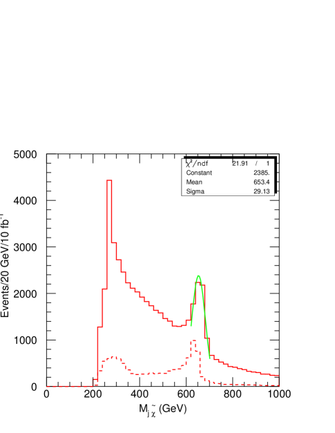
Figure 31: $\tilde{\chi}_{2}^{0}$-$q$ mass distribution at point G2b. Events have a lepton and a slepton with invariant mass in a $\pm 5$ GeV window around the $\tilde{\chi}_{2}^{0}$. The dashed distribution corresponds to cases where the jet is from a $b$-quark.The fit is a Gaussian over the range 625 to 700 GeV

The decay $\tilde{q}_{L}\to\tilde{\chi}_{2}^{0}q$ is significant but not dominant. It can be reconstructed by selecting events that have a $\ell\tilde{\ell}$ mass within 5 GeV of the $\tilde{\chi}_{2}^{0}$ peak in Figure 27 and combining the $\tilde{\chi}_{2}^{0}$ momentum with the momentum of any of the four highest $p_{T}$ jets. The resulting mass distribution of the jet-$\tilde{\chi}_{2}^{0}$ system is shown in Figure 31; it has a somewhat wider peak than that of Figure 30 a little below the average $\tilde{q}_{L}$ mass of $674\,{\rm GeV}$. The signal to background ratio is poorer than in Figure 30, a reflection of the smaller branching ratio $\tilde{q}_{L}\to\tilde{\chi}_{2}^{0}q$ ($\sim 25\%$).

It is also possible to reconstruct the $\tilde{b}_{1,2}$ squarks, The subset of events in Figure 31 for which the jet is tagged as a $b$ jet is shown in Figure 31 as the dashed curve. No correction of the $b$-jet energy is done. The $\tilde{b}$ squark peak is clearly visible and is at somewhat lower masses. The resolution is insufficient to separate the peaks from $b_{1}$ and $b_{2}$ whose average mass is 647 GeV and separation is 9 GeV. A subset of the events of Figure 30 where the quark jet is tagged as a $b$-jet is shown as the dashed line in Figure 30. No structure is visible in this case. This difference is due to the branching ratios; $BR(\tilde{b_{1}}\to{\tilde{\chi}_{1}^{0}}b)=5.9\%$, $BR(\tilde{b_{2}}\to{\tilde{\chi}_{1}^{0}}b)=3.6\%$, $BR(\tilde{q_{R}}\to{\tilde{\chi}_{1}^{0}}q)=94\%$, while $BR(\tilde{b_{1}}\to\tilde{\chi}_{2}b)=15.6\%$, $BR(\tilde{b_{2}}\to\tilde{\chi}_{2}b)=10.8\%$, and $BR(\tilde{q_{l}}\to\tilde{\chi}_{2}q)=25\%$. The mixing between the b-squarks ensures that both can decay to $\tilde{\chi}_{2}$.

The wider peak of Figure 31 relative to that of Figure 30 can now be understood. It is due to the presence of a significant number of $b$-squarks in the former distribution. The mass differences between $\tilde{q}_{L}$ and $\tilde{b}$ are not large enough for the peaks to separate and the result is a broad distribution.

5.6 Reconstruction of $\tilde{\tau}\tau$ Decays

The decay $\tilde{\chi}_{i}^{0}\to{\tilde{\tau}}^{\pm}\tau^{\mp}$ is more difficult to reconstruct than $\tilde{\chi}_{i}^{0}\to{\tilde{\ell}}_{R}^{\pm}\ell^{\mp}$, but it can provide information on the gaugino content of the $\tilde{\chi}_{i}^{0}$. A technique similar to that discussed in Refs.  and can be used. Hadronic $\tau$’s are selected with visible $p_{T}>20\,{\rm GeV}$ and $\eta<2.5$. These are identified by taking jets where the number of charged tracks is less than or equal to three. The simplest approach is to combine the visible $\tau$ momentum with the slepton momentum. The resulting mass distributions are shown in Figure 32 and on an expanded scale for masses near the ${\tilde{\chi}_{1}^{0}}$ mass in Figure 33. These curves do not have true peaks because of the missing $\nu_{\tau}$, but they do have fairly sharp endpoints at the ${\tilde{\chi}_{1}^{0}}$ and $\tilde{\chi}_{2}^{0}$ masses.

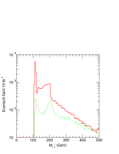
Figure 32: ${\tilde{\tau}}$-$\tau$ mass distribution at Point G2b. Solid curve: Using visible $\tau$ momentum. The dotted curve is obtained by selecting events where the missing $E_{T}$ is aligned with the tau direction by $\Delta\phi<0.1\pi$ and adding $\hbox to0.0pt{\hbox to7.95831pt{\hfil/\hfil}\hss}E_{T}$ to $\tau$ momentum.

Figure 33: Same as Figure 32 on a finer scale with smaller bins.

If the slepton momenta are included in the calculation of $\hbox to0.0pt{\hbox to7.95831pt{\hfil/\hfil}\hss}E_{T}$ and there are no other neutrinos, then $\hbox to0.0pt{\hbox to7.95831pt{\hfil/\hfil}\hss}E_{T}$ can be used to determine the true $\tau$ momentum. Only the highest $p_{T}$ $\tau$ is used, and the angle between it and the $\hbox to0.0pt{\hbox to7.95831pt{\hfil/\hfil}\hss}E_{T}$ direction is required to be $\Delta\phi<0.1\pi$. The visible $\tau$ momentum is then scaled by a factor $1+\hbox to0.0pt{\hbox to7.95831pt{\hfil/\hfil}\hss}E_{T}/E_{T,\tau}$, and the ${\tilde{\tau}}$-$\tau$ mass is recomputed. This gives the dashed curves in Figures 32 and 33. As expected, including $\hbox to0.0pt{\hbox to7.95831pt{\hfil/\hfil}\hss}E_{T}$ not only reduces the statistics but also worsens the resolution for ${\tilde{\chi}_{1}^{0}}$, since the $\tau$ is very soft in this case. However, it produces a peak near the right position for the $\tilde{\chi}_{2}^{0}$. While this peak probably does not improve the mass resolution, it adds confidence that one is seeing a two-body resonance.

5.7 Direct production of electro-weak sparticles

We now return to the events present in the peak at low $M_{\rm eff}$ shown in Figure 24. As pointed out above these events are due to the direct production of gauginos and sleptons. We begin with the event sample used in Figure 28 and remake that distribution with the requirement that $M_{\rm eff}<100$ GeV. This is shown in Figure 34. This plot has a very strong peak at the mass of ${\tilde{\chi}_{1}^{0}}$ and a weak, though still clear one, at the mass of $\tilde{\chi}_{2}^{0}$. This higher peak is suppressed as the lepton from its decay is contributing to $M_{\rm eff}$ and the cut throws away some signal.

Figure 34: Same as Figure 27 except that the additional requirement $M_{\rm eff}<100$ GeV has been made.

Figure 35: The mass of the slepton-lepton-lepton system formed by selecting events in the mass range 110–120 GeV from Figure 34 and combining this slepton-lepton pair with and additional lepton.

We can also repeat the analysis of section 5.4, with the addition of the cut $M_{\rm eff}<100$ GeV. We can take the events in the ${\tilde{\chi}_{1}^{0}}$ peak (in the mass range 110–120 GeV) of Figure 34 and then combine that reconstructed ${\tilde{\chi}_{1}^{0}}$ momentum with an additional charged lepton. The mass distribution of the resulting system is shown in Figure 35. This plot shows a peak at 204 GeV which corresponds to the decay $\tilde{\ell}_{L}\to{\tilde{\chi}_{1}^{0}}\ell\to\tilde{\ell}_{R}^{\pm}\ell^{\mp}\ell$. The fit shown on this plot is a linear combination of a exponential, a Gaussian and constant over the mass range 135–250 GeV. The slepton peak is visible, although there are many fewer events than in Figure 29. The kinematic feature from the decay chain $\tilde{\chi}_{1}^{\pm}\to\tilde{\nu}\ell\to{\tilde{\chi}_{1}^{0}}\nu\ell\to\tilde{\ell}_{R}^{\pm}\ell^{\mp}\nu\ell$ is still visible.

6 Determining SUSY parameters

Once a number of quantities have been measured, we can attempt to determine the particular SUSY model and the values of the parameters. The strategy will be to attempt to perform a global fit to the model parameters using all of the available data, much as the Standard Model is tested using the $W$ and $Z$ masses and the many quantities precisely measured by LEP/SLC. Such a fit is beyond the scope of our work, and we adopt a simpler procedure. We assume that from measurements of global parameters such as those discussed in section 2 we know the approximate scale of the superpartner masses and have some idea that we might be in a GMSB model. The object is then to determine the parameters of that model and check its consistency. We must therefore determine the parameters $\Lambda$, $M_{m}$, $N_{5}$, $\tan\beta$ and $\mathop{\rm sgn}\mu$ and $C_{\rm grav}$. If we know the value of one gaugino and one squark or slepton mass of the first two generations measured at the mass scale $M_{m}$ then $N_{5}$ and $\Lambda$ are determined. Since these are measured at the a lower energy scale, the physical masses also depend on $M_{m}$ via the renormalization group scaling and we need one more measurement to constrain it’s value. Two gaugino masses and one squark or slepton mass of the first two generations suffice. $\tan\beta$ can be constrained either from the Higgs mass or from the masses of the third generation squarks and sleptons. In the case of model G2b, the splitting between $\tilde{e}_{R}$ and $\tilde{\tau}_{1}$ constrains it. Additional constraints on $\tan\beta$ and on $\mathop{\rm sgn}\mu$ arise from the Higgs, $\tilde{\chi}_{i}^{0}$ and $\tilde{\chi}_{i}^{\pm}$ masses. The only constraint upon $C_{\rm grav}$ arises from the lifetime of the NLSP. In cases G1a and G2a and G2b we have precise measurements of the slepton and $\chi_{2}^{0}$ and $\chi_{1}^{0}$ masses, so the less precise measurements of the squark and gluino masses are not useful in determining the fundamental parameters; they only provide powerful consistency checks. Indeed the case G2b has so many observables, that it is enormously over constrained.

In addition to the measurements presented above we assume that the lightest Higgs boson has its mass determined precisely from its decay to gamma-gamma. We will assume two values for its error; $\pm 3$ GeV, which we estimate is the current systematic limit in the theoretical calculations needed to relate it to the model parameters; and $\pm 100$ MeV which corresponds to the expected experimental precision.

Our strategy for determining the parameters is as follows. We choose a point randomly in parameter space and compute the spectrum. We assign a probability to this point determined from how well it agrees with our “measured quantities” using our estimates of the errors on those quantities. The process is repeated for many points and the probabilities used to determine the central values of the parameters, their errors and their correlations. $N_{5}$ is treated as a continuous variable for these purposes.

At Point G1a the measurements discussed above for 10 (30) fb^-1 where statistical errors will still be important, viz.

• $M_{\tilde{\chi}_{2}^{0}}\sqrt{1-\left(M_{{\tilde{\ell}}_{R}}\over M_{\tilde{\chi}_{2}^{0}}\right)^{2}}\sqrt{1-\left(M_{{\tilde{\chi}_{1}^{0}}}\over M_{{\tilde{\ell}}_{R}}\right)^{2}}=105.1\pm 0.10(0.10)\,{\rm GeV}$ ,

• $\sqrt{M_{\tilde{\chi}_{2}^{0}}^{2}-M_{\chi_{1}^{0}}^{2}}=189.7\pm 0.50(0.30)$ GeV,

• $\sqrt{M_{\ell_{R}}^{2}-M_{\chi_{1}^{0}}^{2}}=112.7\pm.20(0.15)$ GeV

• $\sqrt{M_{\chi_{2}^{0}}^{2}-M_{\ell_{R}}^{2}}=152.6\pm.50(0.30)$ GeV

• $m_{h^{0}}=109.47\pm 3$ GeV,

imply that

• $\Lambda=90000\pm 1800(1200)$ GeV,

• $M_{m}=500000\pm 150000(120000)$ GeV,

• $\tan\beta=5.0\pm 1.5(0.9)$,

• $N_{5}=1\pm 0.012(0.10)$.

$\mathop{\rm sgn}\mu$ is determined unambiguously. Some improvement will be possible with greater integrated luminosity until the systematic limit is reached. This will occur for 100 fb^-1 of integrated luminosity. Assuming that the errors are then $\pm 100$ MeV, $\pm 200$ MeV, $\pm 100$ MeV, $\pm 200$ MeV and $\pm 3$ GeV respectively, the uncertainties on the parameters reduce:

• $\Lambda=90000\pm 630$ GeV,

• $M_{m}=500000\pm 80000$ GeV,

• $\tan\beta=5.0\pm 0.3$,

• $N_{5}=1\pm 0.008$.

If the error on the Higgs mass is reduced to $\pm 100$ MeV, the uncertainty on $\tan\beta$ reduces to $\pm 0.1$; the other uncertainties are unchanged. The poorer precision on $M_{m}$ reflects the fact that it enters only via the renormalization group evolution and therefore that the observed masses depend only logarithmically upon it.

At Point G1b, we have for 10 fb^-1 of integrated luminosity

• $M_{\tilde{\chi}_{2}^{0}}\sqrt{1-\left(M_{{\tilde{\ell}}_{R}}\over M_{\tilde{\chi}_{2}^{0}}\right)^{2}}\sqrt{1-\left(M_{{\tilde{\chi}_{1}^{0}}}\over M_{{\tilde{\ell}}_{R}}\right)^{2}}=105.1\pm 0.10\,{\rm GeV}$,

• $m_{\tilde{g}}-m_{\tilde{\chi}_{2}^{0}}=523\pm 50$ GeV,

• $m_{h^{0}}=109.47\pm 3$ GeV,

The precision on the second of these numbers can be expected to increase with more integrated luminosity; the others are systematics limited. These are sufficient only to constrain the following with any degree of precision

• $\Lambda N_{5}=90000\pm 860$ GeV,

• $\tan\beta=5.0^{+1.9}_{-1.3}$

This is due to an accident in our choice of parameters. The position of the kinematic endpoint of Figure 11 is insensitive to variations of the slepton mass, when $m_{\tilde{\ell}_{R}}=\sqrt{m_{\tilde{\chi}_{2}^{0}}m_{{\tilde{\chi}_{1}^{0}}}}$. For our choice of parameters these quantities differ by 0.5 GeV! As ${\tilde{\chi}_{1}^{0}}$ and $\tilde{\chi}_{0}^{2}$ are almost purely gaugino, these relations provide constraints only on the gaugino masses, i.e. on the product $\Lambda N_{5}$. If we assume that the we are able to constrain the average light squark mass within 50 GeV of its nominal value as appears to be possible from the discussion surrounding Figure 15, for 30 fb^-1, we then obtain

• $\Lambda N_{5}=90000\pm 620$ GeV,

• $\Lambda=90000\pm 8100$ GeV,

• $M_{m}<7\times 10^{8}$ GeV (95% confidence)

• $\tan\beta=5.0^{+1.9}_{-1.3}$

Here we have restricted $M_{m}>\Lambda$; the model is not sensible if this is not the case. If the error on the Higgs mass is reduced to $\pm 100$ MeV, the uncertainty on $\tan\beta$ reduces to $\pm 0.1$; the other uncertainties do not reduce. It is not possible to determine $\mathop{\rm sgn}\mu$ using the signals that we have shown. For example, the set of parameters $\Lambda=104500$ GeV, $M_{m}=0.239\times 10^{9}$ GeV, $N_{5}=0.872$ and $\mathop{\rm sgn}\mu=-1$ is acceptable. The mass of $\tilde{\chi}_{2}^{0}$ (${\tilde{\chi}_{1}^{0}}$) is increased by 19 (6) GeV and the mass of $\tilde{e}_{R}$ by 40 GeV, but this case has the same end point in Figure 11. An independent constraint on the slepton mass or a measurement of the squark mass with a precision of order 10 GeV is needed to eliminate this case.

At Point G2a the measurements discussed above for 10 fb^-1 viz.

• $\sqrt{m_{\tilde{\chi}_{1}^{0}}^{2}-m_{\tilde{e}_{R}}^{2}}=52.21\pm 0.07$ GeV,

• $\sqrt{m_{\tilde{\chi}_{2}^{0}}^{2}-m_{\tilde{\mu}_{R}}^{2}}=175.94\pm 0.27$ GeV,

• $\sqrt{m_{\tilde{q}_{R}}^{2}-m_{\tilde{e}_{R}}^{2}}=640\pm 7$ GeV,

• $\sqrt{m_{\tilde{q}_{R}}^{2}-m_{\tilde{e}_{R}}^{2}}\sqrt{1-{M_{{\tilde{\ell}}_{R}}^{2}\over M_{{\tilde{\chi}_{1}^{0}}}^{2}}}/\sqrt{M_{\tilde{q}_{R}}^{2}-M_{{\tilde{\chi}_{1}^{0}}}^{2}}=0.45\pm 0.004$

• $m_{h^{0}}=106.61\pm 3$ GeV,

imply that

• $\Lambda=30000\pm 410$ GeV,

• $M_{m}=250000\pm 44000$ GeV,

• $\tan\beta=5.0\pm 0.7$

• $N_{5}=3\pm 0.036$.

$\mathop{\rm sgn}\mu$ is determined unambiguously. Only small improvements can be expected as the integrated luminosity is increased above 10 fb^-1. If we reduce the errors on the first two quantities to 50 and 180 MeV respectively, their likely systematic limits, as might be achieved with 30 fb^-1 of data we obtain

• $\Lambda=30000\pm 380$ GeV,

• $M_{m}=250000\pm 42000$ GeV,

• $\tan\beta=5.0\pm 0.7$

• $N_{5}=3\pm 0.035$.

If the error on the Higgs mass were reduced to $\pm 100$ MeV, the error on $\tan\beta$ reduces to $\pm 0.04$.

At Point G2b the measurements discussed above viz.

• $m_{\tilde{e}_{R}}=102.67\pm 0.1$ GeV,

• $m_{\tilde{\mu}_{R}}=102.67\pm 0.1$ GeV,

• $m_{\tilde{\tau}_{1}}=101.35\pm 0.1$ GeV,

• $m_{{\tilde{\chi}_{1}^{0}}}=115.18\pm 0.1$ GeV,

• $m_{\tilde{\chi}_{2}^{0}}=203.71\pm 0.2$ GeV, and

• $m_{h^{0}}=106.61\pm 3$ GeV,

imply that

• $\Lambda=30000\pm 175$ GeV

• $M_{m}=250000\pm 22500$

• $\tan\beta=5.0\pm 0.21$

• $N_{5}=3\pm 0.014$.

$\mathop{\rm sgn}\mu$ is determined unambiguously. These measurements are likely to be at their systematic limits with 10 fb^-1 of integrated luminosity and further improvement will be difficult. If the error on the Higgs mass is reduced to $\pm 100$ MeV, the error on $\tan\beta$ reduces to $\pm 0.02$.

In case G1b whose global signatures are similar to SUGRA, we must address the issue of whether it could be confused with a SUGRA model. We search SUGRA parameter space for test of parameters that could be consistent with the following:

• $M_{\tilde{\chi}_{2}^{0}}\sqrt{1-\left(M_{{\tilde{\ell}}_{R}}\over M_{\tilde{\chi}_{2}^{0}}\right)^{2}}\sqrt{1-\left(M_{{\tilde{\chi}_{1}^{0}}}\over M_{{\tilde{\ell}}_{R}}\right)^{2}}=105.1\pm 0.10\,{\rm GeV}$,

• $m_{\tilde{g}}-m_{\tilde{\chi}_{2}^{0}}=523\pm 50$ GeV,

• $m_{h^{0}}=109.47\pm 3$ GeV,

• $m_{\tilde{q}}-m_{\tilde{g}}=200\pm 500$ GeV.

We obtain the following solution for the SUGRA parameters

• $m_{0}=100\pm 20$ GeV

• $m_{1/2}=295\pm 6$ GeV

• $\tan\beta=4.5\pm 1.1$

• $\mathop{\rm sgn}\mu=+1$

• $A=250\pm 200$ GeV

This solution has only a 15% probability. The central value of the light squark masses for this solution is 760 GeV. Most of the other masses are similar to those of case G1b with the exception of $\tilde{e}_{L}$ which has mass 100 GeV larger. This result illustrates the general difference between SUGRA and GMSB models. The mass splitting between the squarks and $\tilde{e}_{R}$ is larger in the GMSB case. If we assume that $m_{\tilde{q}}-m_{\tilde{g}}=200\pm 75$ GeV as we might expect from the methods of Section 3 with at least 30 fb^-1 of integrated luminosity, then the SUGRA solution is eliminated (it has $10^{-5}$ probability) and the ambiguity resolved.

7 Discussion and Conclusions

In this paper we have given examples of how LHC experiments might analyze supersymmetry events if SUSY exists and if the pattern of superpartner masses is given by gauge mediated models of supersymmetry breaking. We have illustrated the four classes of phenomenology to be expected in such models: events with missing energy that are similar to those expected in SUGRA models (Point G1b); events with a pair of isolated photons from ${\tilde{\chi}_{1}^{0}}$ decay (Point G1a); events with long lived sleptons (Point G2b); and events with leptons from prompt slepton decay (Point G2a). In the first case, we have discussed how measurements can be made which enable one to prove that the gauge mediated model and not SUGRA is responsible for the pattern of masses. In the other cases, detection and measurement is easier than in SUGRA. Characteristic features are present such as photons, leptons or stable charged particles, that enable the supersymmetry signals to be extracted trivially from Standard Model backgrounds. In addition, these features make it possible to identify and use longer decay chains.

We have illustrated a technique whereby the supersymmetry events can be fully reconstructed despite the presence of two undetected particles. The technique relies upon there being a decay chain of sufficient length that occurs twice in the same event. Each step in the chain provides a constraint and sufficient constraints can occur that together with the measurement of $\hbox to0.0pt{\hbox to7.95831pt{\hfil/\hfil}\hss}E_{T}$ enables the event to be reconstructed. In such cases the masses of the superparticles in the decay chain can be measured directly rather than inferred from kinematic distributions.

In all of the cases discussed in this paper, as in the SUGRA cases discussed previously  [1, 2, 3], the LHC will be capable of making many precise measurements that will enable the underlying model of supersymmetry to be severely constrained should supersymmetric particles be observed. The key to all of these analyses is the ability to identify a characteristic final state arising from the decay of a sparticle that is copiously produced. The main such decays that have been used in the SUGRA and GMSB analyses done so far are:

• Dileptons from $\tilde{\chi}_{2}\to{\tilde{\chi}_{1}^{0}}\ell^{+}\ell^{-}$ or $\tilde{\chi}_{2}\to\tilde{\ell_{R}}\ell_{R}{\tilde{\chi}_{1}^{0}}\ell^{+}\ell^{-}$;

• taus from the decays $\tilde{\chi}_{2}\to{\tilde{\chi}_{1}^{0}}\tilde{\tau_{1}}^{+}\tau_{1}^{-}$ or $\tilde{\chi}_{2}\to\tilde{\tau_{1}}\tau_{1}\to{\tilde{\chi}_{1}^{0}}\tau^{+}\tau^{-}$, which can dominate when $\tan\beta$ is large;

• $\tilde{\chi}_{2}\to{\tilde{\chi}_{1}^{0}}h\to{\tilde{\chi}_{1}^{0}}b\overline{b}$.

In the case of GMSB or $R$-parity breaking models the subsequent decay of ${\tilde{\chi}_{1}^{0}}$ can provide additional information and constraints. Of course the information extracted in this way is only a small fraction of the total available. A complete analysis will involve generating large samples of events for many SUSY models and comparing all possible distributions with experiment.

Appendix

The details of the full reconstruction used in section 2.2 are given here.

Events are selected to have four leptons and two photons with a unique combination of two leptons and one photon coming from each $\tilde{\chi}_{2}^{0}$ decay. The $\tilde{\chi}_{2}^{0}$, ${\tilde{\ell}}_{R}$, and ${\tilde{\chi}_{1}^{0}}$ masses are assumed to be known precisely from the distributions discussed in section 2.1, and the ${\tilde{G}}$ mass was assumed to be (essentially) zero. This leads to the following set of equations for the 4-momentum $p$ of the gravitino:

$$p^{2} = 0$$

$$(p+p_{\gamma})^{2} = M_{{\tilde{\chi}_{1}^{0}}}^{2}\,,$$

$$(p+p_{\gamma}+p_{\ell_{2}})^{2} = M_{{\tilde{\ell}}}^{2}\,,$$

$$(p+p_{\gamma}+p_{\ell_{2}}+p_{\ell_{1}})^{2} = M_{\tilde{\chi}_{2}^{0}}^{2}\,.$$

This implies that the gravitino momentum $p$ is given in terms of the photon momentum $k$ and the lepton momenta $l$ and $q$ by

$$2p_{0}k_{0}-2\vec{p}\cdot\vec{k} = M_{{\tilde{\chi}_{1}^{0}}}^{2}\equiv C_{k}\,,$$

$$2p_{0}l_{0}-2\vec{p}\cdot\vec{l} = M_{{\tilde{\ell}}_{R}}^{2}-M_{{\tilde{\chi}_{1}^{0}}}^{2}-2k\cdot l\equiv C_{l}\,,$$

$$2p_{0}q_{0}-2\vec{p}\cdot\vec{q} = M_{\tilde{\chi}_{2}^{0}}^{2}-M_{{\tilde{\ell}}_{R}}^{2}-2(k+l)\cdot q-q^{2}\equiv C_{q}\,,$$

where

$$p_{0}=\sqrt{\vec{p}}\,.$$

It is now clear that they give two linear and one quadratic constraint and hence an additional $2\times 2$ ambiguity. The solution is straightforward. From the above equations one finds

$$\vec{p}\cdot\vec{D}_{1} = E_{1}\,,$$

$$\vec{p}\cdot\vec{D}_{2} = E_{2}\,,$$

where

$$\vec{D}_{1} = 2l_{0}\vec{k}-2k_{0}\vec{l}\,,$$

$$E_{1} = -l_{0}C_{k}+k_{0}C_{l}\,,$$

$$\vec{D}_{2} = 2q_{0}\vec{k}-2k_{0}\vec{q}\,,$$

$$E_{1} = -q_{0}C_{k}+k_{0}C_{q}\,.$$

These can be solved to give

$$p_{i}=F_{i}+G_{i}p_{z},\quad i=1,2\,,$$

where

$$F_{x} = {E_{1}D_{2y}-E_{2}D_{1y}\over D_{1x}D_{2y}-D_{2x}D_{1y}}\,,$$

$$G_{x} = -{D_{1z}D_{2y}-D_{2z}D_{1y}\over D_{1x}D_{2y}-D_{2x}D_{1y}}\,,$$

$$F_{y} = {E_{1}D_{2x}-E_{2}D_{1x}\over D_{1y}D_{2x}-D_{2y}D_{1x}}\,,$$

$$G_{y} = -{D_{1z}D_{2x}-D_{2z}D_{1x}\over D_{1y}D_{2x}-D_{2y}D_{1x}}\,.$$

This is then substituted into the first of the original equations to yield a quadratic equation for $p_{z}$,

$$H_{0}+H_{1}p_{z}+H_{2}p_{z}^{2}=0\,,$$

where

$$H_{0} = 4k_{0}^{2}(F_{x}^{2}+F_{y}^{2}+M_{\tilde{\chi}_{1}^{0}}^{2})-(C_{k}+2F_{x}k_{x}+2F_{y}k_{y})^{2}\,,$$

$$H_{1} = 4k_{0}^{2}(2F_{x}G_{x}+2F_{y}G_{y})-2(C_{k}+2F_{x}k_{x}+2F_{y}k_{y})(2G_{x}k_{x}+2G_{y}k_{y}+2k_{z})\,,$$

$$H_{2} = 4k_{0}^{2}(G_{x}^{2}+G_{y}^{2}+1)-(2G_{x}k_{x}+2G_{y}k_{y}+2k_{z})^{2}\,.$$

This gives two solutions for the ${\tilde{G}}$ momentum $p$ for a given assignment of the other momenta provided $H_{1}^{2}-4H_{0}H^{2}\geq 0$ and no solution otherwise.

References

- [1] I. Hinchliffe et al. Phys. Rev. D55, 5520 (1997).
- [2] E. Richter-Was et al., ATLAS Internal Note PHYS-No-108; I Hinchliffe et al.ATLAS Internal Note PHYS-No-109; G. Polesello, et al.ATLAS Internal Note PHYS-No-111; S. Abdullin, et al., (CMS Collaboration) CMS-NOTE-1998-006.
- [3] F. Gianotti, ATLAS Internal Note PHYS-No-110.
- [4] L. Alvarez-Gaume, J. Polchinski and M.B. Wise, Nucl. Phys. B221, 495 (1983); L. Ibañez, Phys. Lett. 118B, 73 (1982); J.Ellis, D.V. Nanopolous and K. Tamvakis, Phys. Lett. 121B, 123 (1983); K. Inoue et al. Prog. Theor. Phys. 68, 927 (1982); A.H. Chamseddine, R. Arnowitt, and P. Nath, Phys. Rev. Lett., 49, 970 (1982).
- [5] For reviews see, H.P. Nilles, Phys. Rep. 111, 1 (1984); H.E. Haber and G.L. Kane, Phys. Rep. 117, 75 (1985).
- [6] H. Baer, C.-H. Chen, F. Paige, and X. Tata, Phys. Rev. D52, 2746 (1995); Phys. Rev. D53, 6241 (1996).
- [7] L.J. Hall and M. Suzuki, Nucl.Phys. B231, 419 (1984).
- [8] J. Soderqvist, ATL-PHYS-98-122; E. Nagy in preparation.
- [9] M. Dine, W. Fischler and M. Srednicki, Nucl. Phys. B189, 575 (1981); S. Dimopoulos and S. Raby, Nucl. Phys. B192, 353 (1981); C. Nappi and B. Ovrut, Phys. Lett.113B, 175 (1982); L. Alvarez-Gaumé, M. Claudson and M. Wise, Nucl. Phys. B207, 96 (1982); M. Dine and A. Nelson, Phys. Rev. D48, 1227 (1993); M. Dine, A. Nelson and Y. Shirman, Phys. Rev. D51, 1362 (1995); M. Dine, et al., Phys. Rev. D53, 2658 (1996).
- [10] G.F. Giudice, R. Rattazzi CERN-TH-97-380, hep-ph/9801271 (1998); C Kolda, Nucl. Phys. P. Suppl. 62, 266 (1998).
- [11] S. Raby and K. Tobe, hep-ph/9807281; G. R. Farrar, Nucl. Phys. Proc. Suppl. 62, 485 (1998).
- [12] J. L. Feng and T. Moroi, Phys.Rev. D58, 5875 (1998)
- [13] F. Paige and S. Protopopescu, in Supercollider Physics, p. 41, ed. D. Soper (World Scientific, 1986); H. Baer, F. Paige, S. Protopopescu and X. Tata, in Proceedings of the Workshop on Physics at Current Accelerators and Supercolliders, ed. J. Hewett, A. White and D. Zeppenfeld, (Argonne National Laboratory, 1993).
- [14] ATLAS Collaboration, Technical Proposal, LHCC/P2 (1994).
- [15] CMS Collaboration, Technical Proposal, LHCC/P1 (1994).
- [16] F. James, CERN Program Library Long Writeup D506 (1998).
- [17] A. Nisati, S. Petrarca, and G. Salvini, hep-ph/9707376, Mod. Phys. Lett. A12, 2213 (1997); A. Nisati; ATL-DAQ-98-083.
- [18] I Hinchliffe and F. Paige, ATLAS Internal Note, in preparation.
- [19] Y. Coadou et al., ATLAS Internal Note ATL-PHYS-98-126.