A supersymmetric resolution of the anomaly in charmless nonleptonic $B$-decays
Debajyoti Choudhury^a,, B. Dutta^b,, Anirban Kundu^a,c
a Mehta Research Institute, Chhatnag Road, Jhusi, Allahabad - 211 019, India
^b Center for Theoretical Physics, Department of Physics, Texas A & M University, College Station, TX 77843, USA
^c Department of Physics, Jadavpur University, Calcutta - 700 032, India

Abstract

We examine the large branching ratio for the process $B\rightarrow\eta^{\prime}K$ from the standpoint of R parity violating supersymmetry. We have given all possible $R_{p}\!\!\!\!\!\!/~{}~{}$ contributions to $B\rightarrow\eta^{\prime}K$ amplitudes. We find that only two pairs of $\lambda^{\prime}$-type $R_{p}\!\!\!\!\!\!/~{}~{}$ couplings can solve this problem after satisfying all other experimental bounds. We also analyze those modes where these couplings can appear, e.g., $B^{\pm}\rightarrow\pi^{\pm}K^{0}$, $B^{\pm,0}\rightarrow K^{*\pm,0}\eta^{(\prime)}$, $B^{\pm}\rightarrow\phi K^{\pm}$ etc., and predict their branching ratios. Further, one of these two pairs of couplings is found to lower the branching ratio of $B^{\pm}\rightarrow\phi K^{\pm}$, thereby allowing larger $\xi\equiv{1\over N_{c}}$. This allows us to fit $B^{\pm}\rightarrow\omega K^{\pm}$ and $B^{\pm}\rightarrow\omega\pi^{\pm}$, which could not be done in the SM framework.

I. Introduction

Recently, the CLEO collaboration has reported the branching ratios (BR) of a number of charmless nonleptonic $B\rightarrow PP$ and $B\rightarrow PV$ two-body decay modes where $P$ and $V$ denote, respectively, a pseudoscalar and a vector meson. Some of these modes have been observed for the first time and the upper bounds on the others have been improved[2, 3].

Among the $B\rightarrow PP$ modes, the branching ratio for $B^{\pm}\rightarrow\eta^{\prime}K^{\pm}$ is found to be larger than that expected within the Standard Model (SM). This result has initated lots of investigations in the last one year [4, 5, 6, 7]. This kind of unexplained puzzle also exists in the $B\rightarrow PV$ modes where it is found that the branching ratios of $B^{\pm}\rightarrow\phi K^{\pm}$, $B^{\pm}\rightarrow\omega\pi^{\pm}$ and $B^{\pm}\rightarrow\omega K^{\pm}$ are hard to fit simultaneously [9, 10]. Present attempts to explain the large branching ratio $BR(B^{\pm}\rightarrow\eta^{\prime}K^{\pm})$ involve large form factors and/or large charm content for $\eta^{\prime}$, with contribution arising from $b\rightarrow s\bar{c}c\rightarrow s\eta^{\prime}(\eta)$, and low strange quark mass [4, 5, 6, 7]. In an interesting paper [11], consequences of large $B\rightarrow\eta^{\prime}K$ branching ratio from purely SU(3) viewpoint has been studied.

In this paper we try to address the large BR problem from the standpoint of $R$-parity ($R_{p}$) violating supersymmetry (SUSY) theories. Motivations for invoking SUSY and its $R_{p}\!\!\!\!\!\!/~{}~{}$ version have been discussed in detail in the literature [12]. Some of its effects on $B$-decays have also been investigated [13]. Since the new interactions modify the SM Hamiltonian, it is natural to revisit these calculations and try to see whether the above mentioned puzzles can be solved. We calculate the QCD-improved short-distance part with the usual operator product expansion and Wilson coefficients (WC), while the long-distance parts are calculated by the factorization technique which is very successful in estimating $B\rightarrow D$ decays. The requirement that any “new physics” solution of the perceived anomaly does not overly affect other observables that are in good agreement with the SM predictions restricts us to two particular sets of couplings within the $R_{p}\!\!\!\!\!\!/~{}~{}$ scenario. Interestingly enough, we find that one of these sets also leads to a better fit for the decays $B^{\pm}\rightarrow\phi K^{\pm}$, $B^{\pm}\rightarrow\omega\pi^{\pm}$ and $B^{\pm}\rightarrow\omega K^{\pm}$.

We organize the letter as follows. In section II, we give a very brief introduction to the SM and $R_{p}\!\!\!\!\!\!/~{}~{}$ Hamiltonian, and list the possible $R_{p}\!\!\!\!\!\!/~{}~{}$ operators that can contribute to charmless decays. We discuss the $B\rightarrow PP$ and $B\rightarrow PV$ decay modes in section III. The new physics contributions to the decay modes $B^{\pm}\rightarrow\eta^{\prime}K^{\pm}$ and $B^{\pm}\rightarrow\eta K^{\pm}$ are shown. In section IV, we discuss how $R_{p}\!\!\!\!\!\!/~{}~{}$ can raise the branching ratio of $B\rightarrow\eta^{\prime}K$ without jeopardizing other decay modes. We make predictions about the yet-to-be-observed channels which can be tested in the upcoming B-factories. We also discuss how to fit the new results in $B\rightarrow PV$ modes in presence of the new couplings which are used to raise the BR of $B\rightarrow\eta^{\prime}K$. We conclude in section V.

2. Effective Hamiltonian for charmless decays

2.1 SM Hamiltonian

The effective Hamiltonian for charmless nonleptonic $B$ decays can be written as

$${\cal H}={G_{F}\over\sqrt{2}}\Big{[}V_{ub}V^{*}_{uq}\sum_{i=1,2}c_{i}O_{i}-V_{tb}V^{*}_{tq}\sum_{i=3}^{12}c_{i}O_{i}\Big{]}+h.c.$$ (1)

The Wilson coefficients (WC), $c_{i}$, take care of the short-distance QCD corrections. We find all our expressions in terms of the effective WCs and refer the reader to the papers [8, 14, 15, 16] for a detailed discussion. We use the effective WCs for the processes $b\rightarrow s\bar{q}q^{\prime}$ and $b\rightarrow d\bar{q}q^{\prime}$ from ref. [8]. The regularization scale is taken to be $\mu=m_{b}$. In our subsequent discussion, we will neglect small effects of the electromagnetic moment operator $O_{12}$, but will take into account effects from the four-fermion operators $O_{1}-O_{10}$ as well as the chromomagnetic operator $O_{11}$.

2.2 The $R_{p}$-violating Hamiltonian

The superpotential of the minimal supersymmetric standard model (MSSM) can contain terms, apart from those obtained by a straightforward supersymmetrization of the SM potential, of the form

$${\cal W}_{R_{p}\!\!\!\!\!\!/~{}~{}}=\kappa_{i}L_{i}H_{2}+\lambda_{ijk}L_{i}L_{j}E_{k}^{c}+\lambda^{\prime}_{ijk}L_{i}Q_{j}D_{k}^{c}+\lambda^{\prime\prime}_{ijk}U_{i}^{c}D_{j}^{c}D_{k}^{c}\,$$ (2)

where $E_{i}$, $U_{i}$ and $D_{i}$ are respectively the $i$-th type of lepton, up-quark and down-quark singlet superfields, $L_{i}$ and $Q_{i}$ are the SU$(2)_{L}$ doublet lepton and quark superfields, and $H_{2}$ is the Higgs doublet with the appropriate hypercharge. Symmetry properties dictate that $\lambda_{ijk}=-\lambda_{jik}$ and $\lambda^{\prime\prime}_{ijk}=-\lambda^{\prime\prime}_{ikj}$. Apparently, the bilinear term can be rotated away with a redefinition of lepton and Higgs superfields, but the effect reappears as $\lambda$s, $\lambda^{\prime}$s and lepton-number violating soft terms [17]. The first three terms of eq.(2) violate lepton number whereas the fourth term violates baryon number. Thus, simultaneous presence of both sets would lead to catastrophic rates for proton decay, and hence it is tempting to invoke a discrete symmetry which forbids all such terms. One introduces the conserved quantum number

$$R_{p}=(-1)^{3B+L+2S}$$

which is $+1$ for the SM particles and $-1$ for their superpartners. However, to prevent proton decay, one needs to forbid only one set, and not necessarily both. This leaves us with the possibility of additional Yukawa interactions within the MSSM, many consequences of which have already been discussed extensively in the literature.

For our purpose, we will assume either $\lambda^{\prime}$ or $\lambda^{\prime\prime}$-type couplings to be present ($\lambda$-type couplings do not lead to nonleptonic decays), but not both. Assuming all $R_{p}\!\!\!\!\!\!/~{}~{}$ couplings to be real, the effective Hamiltonian for charmless nonleptonic $B$-decay can be written as

$$\begin{array}[]{rcl}\displaystyle H_{eff}^{\lambda^{\prime}}(b\rightarrow\bar{d}_{j}d_{k}d_{n})&=&\displaystyle d^{R}_{jkn}[\bar{d}_{n\alpha}\gamma^{\mu}_{L}d_{j\beta}\;\bar{d}_{k\beta}\gamma_{\mu R}b_{\alpha}]+d^{L}_{jkn}[\bar{d}_{n\alpha}\gamma^{\mu}_{L}b_{\beta}\;\bar{d}_{k\beta}\gamma_{\mu R}d_{j\alpha}]\ ,\\[6.45831pt] \displaystyle H_{eff}^{\lambda^{\prime}}(b\rightarrow\bar{u}_{j}u_{k}d_{n})&=&\displaystyle u^{R}_{jkn}[\bar{u}_{k\alpha}\gamma^{\mu}_{L}u_{j\beta}\;\bar{d}_{n\beta}\gamma_{\mu R}b_{\alpha}]\ ,\\[6.45831pt] \displaystyle H_{eff}^{\lambda^{\prime\prime}}(b\rightarrow\bar{d}_{j}d_{k}d_{n})&=&\displaystyle{1\over 2}d^{\prime\prime}_{jkn}[\bar{d}_{k\alpha}\gamma^{\mu}_{R}d_{j\beta}\;\bar{d}_{n\beta}\gamma_{\mu R}b_{\alpha}-\bar{d}_{k\alpha}\gamma^{\mu}_{R}d_{j\alpha}\;\bar{d}_{n\beta}\gamma_{\mu R}b_{\beta}]\ ,\\[6.45831pt] \displaystyle H_{eff}^{\lambda^{\prime\prime}}(b\rightarrow\bar{u}_{j}d_{k}d_{n})&=&\displaystyle u^{\prime\prime}_{jkn}[\bar{u}_{k\alpha}\gamma^{\mu}_{R}u_{j\beta}\;\bar{d}_{n\beta}\gamma_{\mu R}b_{\alpha}-\bar{u}_{k\alpha}\gamma^{\mu}_{R}u_{j\alpha}\;\bar{d}_{n\beta}\gamma_{\mu R}b_{\beta}]\ ,\end{array}$$ (3a)

with

$$\begin{array}[]{rclcrclcl}d^{R}_{jkn}&=&\displaystyle\sum_{i=1}^{3}{\lambda^{\prime}_{ijk}\lambda^{\prime}_{in3}\over 8m_{\tilde{\nu}_{iL}}^{2}},&&d^{L}_{jkn}&=&\displaystyle\sum_{i=1}^{3}{\lambda^{\prime}_{i3k}\lambda^{\prime}_{inj}\over 8m_{\tilde{\nu}_{iL}}^{2}},&&(j,k,n=1,2)\\[6.45831pt] u^{R}_{jkn}&=&\displaystyle\sum_{i=1}^{3}{\lambda^{\prime}_{ijn}\lambda^{\prime}_{ik3}\over 8m_{\tilde{e}_{iL}}^{2}},&&&&&&(j,k=1,\ n=2)\\[6.45831pt] d^{\prime\prime}_{jkn}&=&\displaystyle\sum_{i=1}^{3}{\lambda^{\prime\prime}_{ij3}\lambda^{\prime\prime}_{ikn}\over 4m_{\tilde{u}_{iR}}^{2}},&&u^{\prime\prime}_{jkn}&=&\displaystyle\sum_{i=1}^{2}{\lambda^{\prime\prime}_{ji3}\lambda^{\prime\prime}_{kin}\over 4m_{\tilde{u}_{iR}}^{2}},&&(j=1,2,~{}k=1,~{}n=2).\end{array}$$ (3b)

where $\alpha$ and $\beta$ are colour indices and $\gamma^{\mu}_{R,L}\equiv\gamma^{\mu}(1\pm\gamma_{5})$. The parenthetical remarks on the subscripts concentrate on only the relevant couplings.

As is obvious, data on low energy processes can be used to impose rather strict constraints on many of these couplings [18, 19, 20]. Most such bounds have been calculated under the assumption of there being only one non-zero $R_{p}\!\!\!\!\!\!/~{}~{}$ coupling. From eq.(3a), it is evident that such a supposition precludes any tree-level flavour-changing neutral currents, thus negating the very aim of this paper. However, there is no strong argument in support of only one $R_{p}\!\!\!\!\!\!/~{}~{}$ coupling being nonzero. In fact, it might be argued [19] that a hierarchy of couplings may be naturally obtained on account of the mixings in either of the quark and squark sectors. In this paper we will take a more phenomenological approach and try to find out the values of such $R_{p}\!\!\!\!\!\!/~{}~{}$ couplings for which all available data are satisfied. An important role will be played by the $\lambda^{\prime}_{32i}$ type couplings, the constraints on which are relatively weak.

3. $B\rightarrow PP$ and $PV$ modes

We consider next the matrix elements of the various vector ($V_{\mu}$) and axial vector ($A_{\mu}$) quark currents between generic meson states. For the decay constants of a pseudoscalar ($P$) or a vector ($V$) meson defined through

$$\begin{array}[]{rcl}\langle 0|A_{\mu}|P(p)\rangle&=&\displaystyle if_{P}p_{\mu}\\ \langle 0|V_{\mu}|V(\epsilon,p)\rangle&=&f_{V}m_{V}\epsilon_{\mu}\ ,\end{array}$$ (3da)

we use the following (all values in MeV) [6],

$$f_{\omega}=195,\ f_{K^{*}}=214,\ f_{\rho}=210,\ f_{\pi}=134,\ f_{K}=158,\ f_{\eta_{1}}=1.10f_{\pi},\ f_{\eta_{8}}=1.34f_{\pi}.$$ (3db)

The decay constants of the mass eigenstates $$\eta \eta^{\prime}$$ and are related to those for the weak eigenstates through the relations

$$\begin{array}[]{rclcrcl}f^{u}_{\eta^{\prime}}&=&\displaystyle{f_{8}\over\sqrt{6}}\sin\theta+{f_{1}\over\sqrt{3}}\cos\theta&&f^{s}_{\eta^{\prime}}&=&\displaystyle-2{f_{8}\over\sqrt{6}}\sin\theta+{f_{1}\over\sqrt{3}}\cos\theta\\ f^{u}_{\eta}&=&\displaystyle{f_{8}\over\sqrt{6}}\cos\theta-{f_{1}\over\sqrt{3}}\sin\theta,&&f^{s}_{\eta}&=&\displaystyle-2{f_{8}\over\sqrt{6}}\cos\theta-{f_{1}\over\sqrt{3}}\sin\theta.\end{array}$$

The mixing angle can be inferred from the data on the $\gamma\gamma$ decay modes[21] to be $\theta\approx-22^{\circ}$.

Whereas the only nonzero $B\rightarrow P$ matrix element can be parametrized as

$$\langle P(p^{\prime})|V_{\mu}|B(p)\rangle=\Big{[}(p^{\prime}+p)_{\mu}-{m_{B}^{2}-m_{P}^{2}\over q^{2}}q_{\mu}\Big{]}F_{1}^{B\rightarrow P}+{m_{B}^{2}-m_{P}^{2}\over q^{2}}q_{\mu}F_{0}^{B\rightarrow P}\ ,$$ (3dea)

the $$B\rightarrow V$$ transition is given by

$$\begin{array}[]{l}\langle V(\epsilon,p^{\prime})|(V_{\mu}-A_{\mu})|B(p)\rangle\\ \displaystyle\hskip 10.00002pt={2V\over{m_{B}+m_{V}}}\epsilon_{\mu\nu\alpha\beta}\epsilon^{*\nu}p^{\alpha}p^{\prime\beta}\\ \displaystyle\hskip 10.00002pt+i\left[(m_{B}+m_{V})A_{1}\>\epsilon^{*}_{\mu}+\epsilon^{*}\cdot q\>\left\{-A_{2}\frac{(p+p^{\prime})_{\mu}}{m_{B}+m_{V}}+2m_{V}\frac{q_{\mu}}{q^{2}}\left(A_{0}-A_{3}\right)\right\}\right]\end{array}$$ (3deb)

with $$2m_{V}A_{3}\equiv(m_{B}+m_{V})A_{1}-(m_{B}-m_{V})A_{2} F_{0,1}^{B\rightarrow P} V^{B\rightarrow V} F_{0,1}^{B\rightarrow V} q^{2}\equiv(p-p^{\prime})^{2} F_{1}=F_{0} q^{2}=0 F(m_{P_{2}}^{2})=F(0) B q^{2} m_{B} SU(3)$$. All of the quantities , and have a formfactor behaviour in . Note that at , and, to a very good approximation, we can set for decay formfactors since the dependence is dominated by meson poles at the scale . Flavour then allows us to write

$$\begin{array}[]{rclcrcl}F^{B\rightarrow K,\pi^{\pm}}_{0,1}&=&F\ ,&&F^{B\rightarrow\pi^{0}}_{0,1}&=&\displaystyle{F\over\sqrt{2}}\ ,\\ F^{B\rightarrow\eta^{\prime}}_{0,1}&=&\displaystyle F\left({\sin\theta\over\sqrt{6}}+{\cos\theta\over\sqrt{3}}\right)\ ,&&F^{B\rightarrow\eta}_{0,1}&=&\displaystyle F\left({\cos\theta\over\sqrt{6}}-{\sin\theta\over\sqrt{3}}\right)\ .\end{array}$$ (3dec)

There seems to be considerable variation in the range of $$F 0.33 0.5 F=0.36,|V_{ub}/V_{cb}|=0.07 B\rightarrow\pi\pi B\rightarrow\pi K R_{p}\!\!\!\!\!\!/~{}~{} F B\rightarrow V A_{0} B\rightarrow PV \bar{u}\gamma_{\mu}(1-\gamma_{5})b$$ estimated in the literature. Bauer et al estimate it to be [22] while Deandrea et al get a value of [23]. We find that while within the SM, the combination () yields a good fit to and data [8], introduction of interactions allows larger values of . As for the formfactors, it can easily be ascertained that, of the four, only is relevant for the decays that we are interested in. For the current , we have

$$A_{0}^{B\rightarrow\omega}={G\over\sqrt{2}},\qquad A_{0}^{B\rightarrow K^{*}}=G,\qquad A_{0}^{B\rightarrow\rho}={G\over\sqrt{2}},$$ (3ded)

where we use G=0.28 [6]. The only remaining parameters of interest is the mass of the strange quark for which we use $m_{s}(1~{}{\rm GeV})=165$ MeV leading to $m_{s}(m_{b})=118$ MeV.

3.1 $B^{\pm}\rightarrow\eta^{\prime}(\eta)K^{\pm}$

The effective SM Hamiltonian for this decay and its matrix elements are well-studied and can be found in Refs.[6, 8]. As for the $R_{p}\!\!\!\!\!\!/~{}~{}$ operators, it is easy to see that only six of them may contribute (with none from the $u^{\prime\prime}$ set) and may be expressed in terms of

$$\begin{array}[]{rcl}A_{M_{1}}&=&\langle M_{2}|J_{b}^{\mu}|B\rangle\;\langle M_{1}|J_{l\mu}|0\rangle\\ A_{M_{2}}&=&\langle M_{1}|J_{b}^{{}^{\prime}\mu}|B\rangle\;\langle M_{2}|J^{\prime}_{l\mu}|0\rangle.\end{array}$$

where $J$ and $J^{\prime}$ stand for quark currents and the subscripts $b$ and $l$ indicate whether the current involves a $b$ quark or only the light quarks. Neglecting the annihilation diagrams we have, for the $B\rightarrow\eta K$ matrix elements,

$$\begin{array}[]{rcl}{\cal M}^{\lambda^{\prime}}&=&\displaystyle\left(d^{R}_{121}-d^{L}_{112}\right)\xi A_{\eta}^{u}+\left(d^{L}_{222}-d^{R}_{222}\right)\>\left[\frac{\bar{m}}{m_{s}}\left(A_{\eta}^{s}-A_{\eta}^{u}\right)-\xi A_{\eta}^{s}\right]\\[6.45831pt] &+&\displaystyle\left(d^{L}_{121}-d^{R}_{112}\right)\frac{\bar{m}}{m_{d}}A_{\eta}^{u}+u^{R}_{112}\left[\xi A_{\eta}^{u}-{2m_{K}^{2}A_{K}\over(m_{s}+m_{u})(m_{b}-m_{u})}\right],\end{array}$$ (3defa)

where $$\bar{m}\equiv m^{2}_{\eta}/(m_{b}-m_{s})$$, and

$${\cal M}^{\lambda^{\prime\prime}}=d^{\prime\prime}_{112}(1-\xi)A_{\eta}^{u}.$$ (3defb)

Analogous expressions hold for $B^{\pm}\rightarrow\eta^{\prime}K^{\pm}$ where we have to replace $A^{u}_{\eta}$ by $A^{u}_{\eta^{\prime}}$, $A^{s}_{\eta}$ by $A^{s}_{\eta^{\prime}}$ and $m_{\eta}$ by $m_{\eta^{\prime}}$. We note that $\lambda^{\prime\prime}_{112}$ and $\lambda^{\prime\prime}_{113}$ are bounded to be very small irrespective of the presence of other $R_{p}\!\!\!\!\!\!/~{}~{}$ operators, and hence may be neglected. For the numerical analysis, we take $m_{\eta_{8}}=m_{\eta}$ and $m_{\eta_{1}}=m_{\eta^{\prime}}$.

Mode	$BR\times 10^{5}$	SM theory $\times 10^{5}$	Mode	$BR\times 10^{5}$	SM theory $\times 10^{5}$
$B^{+}\rightarrow\eta^{\prime}K^{+}$	$6.5^{+1.5}_{-1.4}\pm 0.9$	$0.8-4.3$	$B^{0}\rightarrow\eta^{\prime}K^{0}$	$4.7^{+2.7}_{-2.0}\pm 0.9$	$0.7-4.1$
$B^{+}\rightarrow\eta^{\prime}K^{\ast+}$	$<13$	$0.01-0.18$	$B^{0}\rightarrow\eta^{\prime}K^{\ast 0}$	$<3.9$	$0.03-0.18$
$B^{+}\rightarrow\eta K^{+}$	$<1.4$	$0.06-0.14$	$B^{0}\rightarrow\eta K^{0}$	$<3.3$	$0.03-0.14$
$B^{+}\rightarrow\eta K^{\ast+}$	$<3.0$	$0.14-0.31$	$B^{0}\rightarrow\eta K^{\ast 0}$	$<3.0$	$0.1-0.5$
$B^{+}\rightarrow\pi^{+}K^{0}$	$2.3^{+1.1}_{-1.0}\pm 0.4$	$1.1-3.5$	$B^{0}\rightarrow\pi^{0}K^{0}$	$<4.1$	$0.6-1.9$
$B^{+}\rightarrow\pi^{0}K^{+}$	$<1.6$	$1.0-1.4$	$B^{0}\rightarrow\pi^{-}K^{+}$	$1.5^{+0.5}_{-0.4}\pm 0.1$	$1.1-2.1$
$B^{+}\rightarrow\pi^{+}\pi^{0}$	$<2.0$	$0.3-1.3$	$B^{0}\rightarrow\pi^{+}\pi^{-}$	$<1.5$	$0.8-1.5$
$B^{+}\rightarrow\phi K^{+}$	$<0.53$	$0.07-5.0$
$B^{+}\rightarrow\omega K^{+}$	$1.5^{+0.7}_{-0.4}\pm 0.3$	$0.01-3.5$	$B^{+}\rightarrow\omega\pi^{+}$	$1.1^{+0.6}_{-0.5}\pm 0.2$	$0.06-1.7$

Table 1: Branching ratios (or upper bounds) for various $B$-meson decays. Also shown are the theoretical predictions based on the SM only [24].

4. Analysis

We are now ready to discuss our results. Our goal is to explain the branching ratio for the $B^{\pm}\rightarrow\eta^{\prime}K^{\pm}$ decay while satisfying the experimental numbers (limits) for all other related decays (see Table 1). To set the perspective, consider the solid curve in Fig. 1($a$), wherein we have plotted $BR(B^{\pm}\rightarrow\eta^{\prime}K^{\pm})$ as a function of $\xi$. It is quite apparent that only for very small $\xi$ could we hope to reconcile the SM predictions with the observations. One may argue, though, that such a conclusion is unwarranted in view of the uncertainty in other parameters such as $F$, the CKM elements $V_{cb}$ and $V_{ub}$, the angle $\gamma$ of the unitarity triangle, and the strange quark mass .

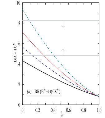
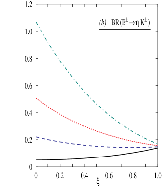
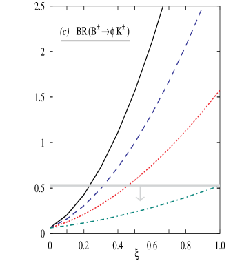
Figure 1: Branching ratios for various decays as a function of  $\xi$. The solid curve gives the SM value. In the presence of a $d^{R}_{222}$ operator with a sfermion mass of 200 GeV, the long-dashed, short-dashed and dot-dashed curves correspond to the cases where each of the two $\lambda^{\prime}$s equal 0.09, 0.07 and 0.05 respectively. The thick lines correspond to the experimental bounds.

Consider instead the ratio $BR(B^{\pm}\rightarrow\eta^{\prime}K^{\pm})/BR(B\rightarrow\pi^{+}K^{0})$ which is independent of $F$ and $V_{cb}$. In Fig. 2, we plot this ratio as a function of $\gamma$ for $\xi=0$, so as to maximize it. Clearly, the SM prediction falls well below the experimental number (remember that $\gamma\sim 0$ is unable to account for the observed CP violation in $K$-system).

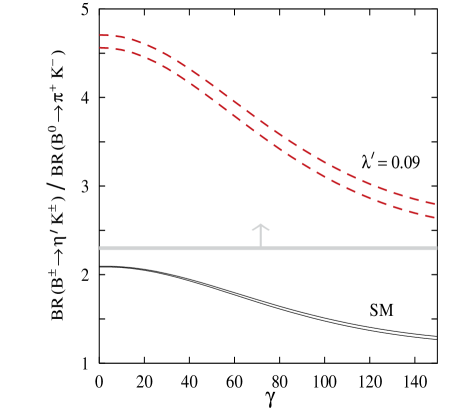
Figure 2: The ratio $BR(B^{\pm}\rightarrow\eta^{\prime}K^{\pm})/BR(B^{0}\rightarrow\pi^{+}K^{-})$ for $\xi=0$ as a function of the CKM parameter $\gamma$. The solid curves represent the SM prediction while the dashed curves are for a $d^{R}_{222}$ with each $\lambda^{\prime}=0.09$. In each case, the upper and lower curves are for $m_{s}(1GeV)=150(165)$ MeV respectively.

Thus, if we demand that $R_{p}\!\!\!\!\!\!/~{}~{}$ solve the $B\rightarrow\eta^{\prime}K$ anomaly, the relevant operators need to add constructively to the SM amplitudes. We make a simplifying assumption here. Rather than consider the most general case, we restrict ourselves to exactly one non-zero product in eq.(3a) and discuss its consequences. This immediately restricts us to particular signs for each of the combinations. To wit, we need one of $d^{R}_{222}$, $d^{R}_{112}$, $u^{R}_{112}$ and $d^{L}_{112}$ to be positive. On the other hand, only negative values for the other four combinations $d^{L}_{222}$, $d^{L}_{121}$, $d^{R}_{121}$ and $d^{\prime\prime}_{112}$ could explain the enhanced BR. We shall concentrate on only the first set.

It is easy to see that $u^{R}_{112}$ also enhances the $BR(B\rightarrow\pi^{+}K^{-})$. Since there exists a stringent experimental bound on this mode, the largest allowed value for $u^{R}_{112}$ is too small to explain the $BR(B\rightarrow\eta^{\prime}K)$. Similarly, the small enhancement due to $d^{L}_{112}$, which occurs only for large value of $\xi$, is unable to explain the anomaly. Thus, we are left with only two terms, namely $d^{R}_{222}$ and $d^{R}_{112}$.

Let us first focus on $d^{R}_{222}$. In all our subsequent discussions, we take, without any loss of generality, both the $\lambda^{\prime}$s in the product $d^{R}$ to be equal, and the intermediate $i$-th sneutrino mass to be 200 GeV. As is evident from eq. 3a, the new physics contribution is proportional to ${\lambda^{\prime}}^{2}/m_{\tilde{\nu}_{iL}}^{2}$. Since the products $\lambda^{\prime}_{122}\lambda^{\prime}_{123}$ and $\lambda^{\prime}_{222}\lambda^{\prime}_{223}$ have a stronger experimental upper bound than the numbers we need, the only possible solution is for $i=3$, i.e., $\lambda^{\prime}_{322}\lambda^{\prime}_{323}$. Similar conclusions follow for $d^{R}_{112}$.

In Figs. (1$a$) and (1$b$), we show the effect of a non-zero $d^{R}_{222}$ on two particular BRs, namely those for $B^{\pm}\rightarrow\eta^{\prime}K^{\pm}$ and $B^{\pm}\rightarrow\eta K^{\pm}$. Clearly, a resolution of the anomaly is now possible, albeit for a $\lambda^{\prime}$-dependent range for $\xi$. Since the $R_{p}\!\!\!\!\!\!/~{}~{}$ contribution to the decay amplitude tends to become too large with increasing $\lambda^{\prime}$, progressively larger values of $\xi$ are required. As for the other modes, it is easy to see that the our solutions respect the experimental numbers/constraints. For example, with $\lambda^{\prime}=0.09(0.07)$ and $\xi=0.2(0.3)$, we expect $BR(B^{0}\rightarrow\eta^{\prime}K^{0})=5(5.5)\times 10^{-5}$, well in consonance with observations (Table 1). Similarly, the BRs for the modes $B^{+}\rightarrow\eta K^{*+},\eta^{\prime}K^{*+}$ and $B^{0}\rightarrow\eta K^{0},\eta K^{*0},\eta^{\prime}K^{*0}$ for $\lambda^{\prime}=0.09$ are predicted to be $1.2(0.6),0.5(0.3),0.8(0.4),0.9(0.4),$ and $0.3(0.2)$ ($\times 10^{-5}$) respectively for $\xi=0(0.5)$. In fact, if our explanation be the correct one, we would expect to see the decay $B^{\pm}\rightarrow\eta K^{*\pm}$ quite soon, whereas some of the other modes may be visible in the upcoming B-factories.

At this stage, a comment is in order. For Figs.(1$a,b,c$), we have used $F=0.36$ and $m_{s}(1GeV)=165$ MeV ($m_{s}(m_{b})=118$ MeV), values preferred by the SM fit. However, in the presence of additional interactions, one may use a different set. As Fig. 2 shows, the dependence on $m_{s}$ is marginal. On the other hand, a larger value for $F$ would enhance the BRs. For example, for $F=0.4$, $\xi=0.55$ and each $\lambda^{\prime}=0.09$, the theoretical BRs for the modes $\eta^{\prime}K^{+}$, $\eta^{\prime}K^{0}$, $\eta K^{+}$, $\eta K^{0}$, $\pi^{-}K^{+}$, $\pi^{+}K^{0}$, $\pi^{+}\pi^{-}$ and $\pi^{+}\pi^{0}$ (last four modes do not have any contribution from $d^{R}_{222}$) are $4.9$, $7.6$, $0.6$, $0.7$, $2.1$, $2.8$, $1.1$ and $0.9$ respectively (all in units of $10^{-5}$). This is the maximum value of $F$ that can be used in conjunction with $\xi=0.55$ since ($i$) the prediction for the $\pi^{-}K^{+}$ mode actually saturates the experimental number, and ($ii$) the data on $B\rightarrow\pi\pi$ implies that $F|V_{ub}/V_{cb}|\leq 0.024$ (note that semileptonic decays give $|V_{ub}/V_{cb}|=0.08\pm 0.02$). Of course, the above does not preclude smaller values for $F$: with $F=0.33$, $\xi=0$ and each $\lambda^{\prime}=0.09$, the theoretical predictions for the abovementioned eight modes are $7.8$, $7.6$, $0.9$, $0.7$, $1.8$, $2.9$, $1.1$ and $0.8$ respectively (again, all in units of $10^{-5}$). Anyway, for these numbers, particularly for those in the first set, one can easily see that more and more channels get close to the discovery limit.

What about the $B\rightarrow PV$ modes? As Fig. 1($c$) shows, the SM fit requires $\xi<0.23$. This is in conflict with other $PV$ modes such as $B^{\pm}\rightarrow\omega K^{\pm}$ and $B^{\pm}\rightarrow\omega\pi^{\pm}$. The former requires either $\xi<0.05$ or $0.65<\xi<0.85$ while the latter requires $0.45<\xi<0.85$ [9]. Interestingly, the $d^{R}_{222}$ operator affects $B^{\pm}\rightarrow\phi K^{\pm}$ while the other two decay modes are blind to it. Since this additional contribution interferes destructively with the SM amplitude, $BR(B^{\pm}\rightarrow\phi K^{\pm})$ is suppressed leading to a wider allowed range for $\xi$ (see Fig 1$c$). For example, with $\lambda^{\prime}=0.09$, $\xi$ can be as large as $0.8$, thus allowing for a common fit to all the three ($PV$) modes under discussion. $d^{R}_{222}$ also affects a $VV$ decay modes such as ($B\rightarrow\phi K^{*}$). As this calculation involves a few more model dependent parameters, we do not analyse it here.

Finally, we investigate the consequences for a non-zero $d^{R}_{112}$ as opposed to $d^{R}_{222}$. For brevity’s sake, we present graphs (see Fig. 3) only for $BR(B^{\pm}\rightarrow\eta^{\prime}K^{\pm})$. It is interesting to note that $\lambda^{\prime}>0.05$ is not admissible for any $\xi<1$, as the model predictions become significantly larger than the observed width. As for $B^{0}\rightarrow\eta^{\prime}K^{0}$, the BR is $6.2(4.8)\times 10^{-5}$ for $\xi=0.3$ and $\lambda^{\prime}=0.025(0.02)$ (see Table 1). Indeed, the entire parameter space allowed by $B^{\pm}\rightarrow\eta^{\prime}K^{\pm}$ is also allowed by $B^{0}\rightarrow\eta^{\prime}K^{0}$.

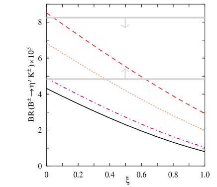
Figure 3: Branching ratio for $B^{\pm}\rightarrow\eta^{\prime}K^{\pm}$ as a function of  $\xi$. The solid curve gives the SM value. In the presence of a $d^{R}_{112}$ operator with a sfermion mass of 200 GeV, the long-dashed, short-dashed and dot-dashed curves correspond to the cases where each of the two $\lambda^{\prime}$s equal 0.025, 0.02 and 0.01 respectively. The thick lines correspond to the experimental bounds.

For such values of $\lambda^{\prime}$s, $BR(B^{\pm}\rightarrow\eta K^{\pm}\mathrel{\hbox to0.0pt{\raise 2.15277pt\hbox{$<$}\hss}{\lower 2.15277pt\hbox{$\sim$}}}3\times 10^{-6}$, and thus well below the experimental upper limit. Similarly, for the other relevant $PP$ modes $B^{0}\rightarrow\eta K^{0},\pi^{0}K^{0}$ and $B^{\pm}\rightarrow K^{\pm}\pi^{0}$, the maximum BRs are $0.15$, $1.9$ and $1.4$ ($\times 10^{-5}$) respectively. Since, for all these decays, the $R_{p}\!\!\!\!\!\!/~{}~{}$ contribution interferes destructively with the SM one, the resultant predictions are considerably suppressed. The best constraints emanate from $BR(B^{\pm}\rightarrow K^{0}\pi^{\pm})$ which supports $0.03<\xi<0.8$ for the $\lambda^{\prime}$s used in Fig. 3.

The case for the $PV$ modes is similar. For the decays $B^{+}\rightarrow\eta K^{*\pm},\eta^{\prime}K^{*\pm},\pi^{0}K^{*\pm}$ and $B^{0}\rightarrow\eta K^{*0},\eta^{\prime}K^{*0},\pi^{0}K^{*0}$ the $R_{p}\!\!\!\!\!\!/~{}~{}$ operator adds constructively whereas for $B^{\pm}\rightarrow K^{0}\rho^{\pm},\pi^{\pm}K^{*0}$ the interference is destructive in nature. The maximum possible BRs for the first six modes, for $\lambda^{\prime}=0.03$ and $\xi=0(0.5)$, are $1.2(1.0),0.75(0.45),0.4(0.3),1.7(1.1),1.0(0.5),0.8(0.4)$ ($\times 10^{-5}$) respectively, smaller than the corresponding experimental numbers. For the last two modes, of course, no question of contradiction with experiment arises.

In short, the modes $B^{\pm}\rightarrow\eta K^{*\pm}$ and $B^{0}\rightarrow\eta K^{*0}$ are close to the discovery limit whereas other modes may have to wait for the next generation B-machines. In a subsequent paper[25], we will discuss the CP violating effect of these $R_{p}\!\!\!\!\!\!/~{}~{}$ operators on all these, and other, modes in detail.

5. Conclusion

To conclude, we have written down all possible $R_{p}\!\!\!\!\!\!/~{}~{}$ SUSY contributions to the effective Hamiltonian for the $B^{\pm}\rightarrow\eta^{\prime}K^{\pm}$ decay. We have found that only two new terms, each involving two $\lambda^{\prime}$-type couplings, can raise the BR to satisfy the experimental number. We have shown that though these two terms appear in other nonleptonic decay modes of the $B$ meson, their BRs always satisfy the experimental constraints in the whole of the allowed parameter space of $\lambda^{\prime}$, $m_{\tilde{\nu}_{iL}}$ and $\xi$. Modes like $\eta K^{*+}$, $\eta K^{*0}$ are close to their discovery limits. Further, one of the new contributions allows larger parameter space in $\xi$ for the decay $B^{\pm}\rightarrow\phi K^{\pm}$, where the other observed modes e.g., $B^{\pm}\rightarrow\omega K^{\pm}$ and $B^{\pm}\rightarrow\omega\pi^{\pm}$ can be fit; this is not possible in the SM framework. This leads us to believe that $B$-decays and upcoming B-factories may be the most promising place to look for new physics beyond the SM.

We thank Amitava Datta and N.G. Deshpande for illuminating discussions.

References

• [1]
• [2] J. Smith (CLEO collaboration), talk presented at the 1997 Aspen winter conference on Particle Physics, Aspen, Colorado, 1997;
M.S. Alam et al.(CLEO collaboration), CLEO CONF 97-23; A. Anastassov et al (CLEO collaboration), CLEO CONF 97-24.
• [3] B.H. Behrens et al.(CLEO collaboration), Phys. Rev. Lett. 80 (1998) 3710;
T. Bergfeld et al.(CLEO collaboration), Phys. Rev. Lett. 81 (1998) 272;
T.E. Browder et al.(CLEO collaboration), Phys. Rev. Lett. 81 (1998) 1786.
• [4] A.L. Kagan and A.A. Petrov, preprint UCHEP-27, UMHEP-443, hep-ph/9707354.
• [5] A. Datta, X.-G. He and S. Pakvasa, Phys. Lett. B419 (1998) 369.
• [6] A. Ali and C. Greub, Phys. Rev. D57 (1998) 2996.
• [7] H.-Y. Cheng and B. Tseng, Phys. Lett. B415 (1997) 263.
• [8] N.G. Deshpande, B. Dutta and S. Oh, Phys. Rev. D57 (1998) 5723.
• [9] N.G. Deshpande, B. Dutta and S. Oh, hep-ph/9712445 (to appear in Phys. Lett. B).
• [10] A. Ali, G. Kramer, C.-D. Lu, hep-ph/9805403.
• [11] A. Dighe, M. Gronau, J.L. Rosner, Phys. Rev. Lett. 79 (1997) 4333.
• [12] H.P. Nilles, Phys. Rep. 110 (84) 1;
H.E. Haber and G.L. Kane, Phys. Rep. 117 (85) 75;
S. Weinberg, Phys. Rev. 26 (82) 287;
N. Sakai and T. Yanagida, Nucl. Phys. B197 (82) 533;
C.S. Aulakh and R. Mohapatra, Phys. Lett. B119 (82) 136.
• [13] D. Guetta, hep-ph/9805274;
D. Guetta, J.M. Mira and E. Nardi, hep-ph/9806359;
T. Feng, hep-ph/9808379.
• [14] A.J. Buras et al., Nucl. Phys. B400 (1993) 37;
A.J. Buras, M. Jamin and M.E. Lautenbacher, ibid. 400 (1993) 75.
• [15] M. Ciuchini et al., Nucl. Phys. B415 (1994) 403.
• [16] R. Fleischer, Z. Phys. C62 (1994) 81; ibid. 58 (1993) 483;
G. Kramer, W. Palmer and H. Simma, Nucl. Phys. B428 (1994) 77.
• [17] I.-H. Lee, Phys. Lett. B138 (1984) 121; Nucl. Phys. B246 (1984) 120;
F. de Campos et al., Nucl. Phys. B451 (1995) 3;
M.A. Diaz, Univ. of Valencia report no. IFIC-98-11 (1998), hep-ph/9802407, and references therein;
S. Roy and B. Mukhopadhyaya, Phys. Rev. D55 (1996) 7020.
• [18] V. Barger, G.F. Giudice and T. Han, Phys. Rev. D40 (1989) 2987;
G. Bhattacharyya and D. Choudhury, Mod. Phys. Lett. A10 (1995) 1699;
M. Hirsch, H.V. Klapdor-Kleingrothaus and S.G. Kovalenko, Phys. Rev. Lett. 75 (1995) 17;
K.S. Babu and R.N. Mohapatra, Phys. Rev. Lett. 75 (1995) 2276.
• [19] C.E. Carlson, P. Roy and M. Sher, Phys. Lett. B357 (1995) 94;
K. Agashe and M. Graesser, Phys. Rev. D54 (1996) 4445;
A.Yu. Smirnov and F. Vissani, Phys. Lett. B380 (1996) 317;
D. Choudhury and P. Roy, Phys. Lett. B378 (1996) 153.
• [20] H. Dreiner, in ‘Perspectives on Supersymmetry’, ed. G.L. Kane (World Scientific), hep-ph/9707435.
• [21] P. Ball, J.M. Frère and M. Tytgat, Phys. Lett. B365 (1996) 367.
• [22] M. Bauer and B. Stech, Phys. Lett. B152 (1985) 380;
M. Bauer, B. Stech and M. Wirbel, Z. Phys. C34 (1987) 103.
• [23] A. Deandrea et al., Phys. Lett. B318 (1993) 549.
• [24] See, e.g., refs. [6, 8]. With different values of $F$, $m_{s}$ and Wilson coefficients, slightly different predictions are obtained by D. Du and L. Guo, Z. Phys. C75 (1997) 9.
• [25] D. Choudhury, B. Dutta and A. Kundu; in preparation.