KEK-TH-606

November 1998

SUSY Phenomenology

Three topics on phenomenology in supersymmetric models are reviewed, namely, the Higgs sector in the supersymmetric model, B and K meson decay in the supergravity model and lepton flavor violation processes in supersymmetric grand unified theory.

1 Introduction

Supersymmetry (SUSY) is a symmetry between fermions and bosons and its theoretical development started from the formulation of SUSY invariant Lagrangian in four dimensional field theory in early ’70s.$\!{}^{{\bf?}}$ Subsequently, SUSY gauge theory, supergravity$\!{}^{{\bf?}}$ and string theory with space-time supersymmetry (supersrting)$\!{}^{{\bf?}}$ were formulated in ’70s.

Phenomenological application of SUSY theory has developed since early ’80s in connection with naturalness problem in the Standard Model (SM). One interesting possibility beyond the SM is an idea that various interactions are unified at very high energy scale. Examples are grand unified theory (GUT) and string unification. In such theories the cutoff energy scale for the SM is considered to be close to the Planck scale ($\sim 10^{19}$ GeV) and the quadratic divergence of the Higgs field in the SM is very problematic because very precise fine tuning between the bare mass term and radiative correction is necessary to ensure that the weak scale is smaller by $10^{16}$ orders than the Planck scale. In SUSY theories this problem can be avoided due to cancellation of the quadratic divergence in scaler mass renormalization. From this point of view SUSY extensions of the SM and the GUT have been extensively studied for more than 15 years.$\!{}^{{\bf?}}$

In the experimental side, the SM has been very successful. LEP and SLAC experiments at the Z pole showed quantitative agreement of various observables with SM predictions. It was also pointed out that three gauge coupling constants determined precisely there are consistent with the SUSY SU(5) GUT assumption although non-SUSY version of the simple SU(5)GUT fails to reproduce the coupling unification.$\!{}^{{\bf?}}$ Since then it has become more and more important to know how one can explore SUSY in the present and future high energy experiments.

In this lecture after a brief introduction to the minimal supersymmetric standard model (MSSM) we discuss three topics on SUSY phenomenology, namely the Higgs sector in SUSY models, B and K meson decay in the supergravity model, and lepton flavor violation (LFV) in SUSY GUT.

2 Minimal Supersymmetric Standard Model

2.1 MSSM Lagrangian

Minimal supersymmetric standard model (MSSM) is a minimal SUSY extension of the SM. In this model we introduce a SUSY partner for each particle in the SM. For left- and right-handed quark and lepton complex scalar fields, squark and slepton, are introduced. The superpartner of gauge boson is gauge fermion (or gaugino) and that of the Higgs field is called higgsino. The superpartners of gluon and SU(2) and U(1) gauge fermions are gluino, wino and bino, respectively. After the electroweak symmetry breaking the wino, bino and higgsino mix each other and form two charged Dirac fermions called chargino and four neutral Majorana fermions called neutralino. As for the Higgs sector the SUSY model contains at least two Higgs doublet fields. This is because different Higgs doublet fields should be introduced for mass terms for the up-type quarks and those for the down-type quarks and charged leptons in order to write appropriate Yukawa couplings without conflict with SUSY. Two Higgs doublets are also required from the gauge anomaly cancellation because the higgsino fields generate additional contributions to the anomaly cancellation condition. The particle content of the MSSM is therefore summarized as two Higgs doublet SM with bosonic superpartners (squarks and sleptons) and fermionic superpartners (gluino, charginos and neutralinos).

The MSSM Lagrangian consists of two parts, SUSY invariant part and soft SUSY breaking terms. General rule of writing SUSY invariant Lagrangian is well known.$\!{}^{{\bf?}}$ There are two kinds of supermultiplets, i.e. gauge supermultiplet which contains gauge fields ($A_{\mu}$) and gauge fermion ($\lambda$) and chiral supermultiplet which consists of a pair of a complex scalar field ($\phi$) and a left-handed Weyl fermion ($\psi$). The SUSY invariant interactions are classified essentially to two kinds, i.e. gauge interactions and superpotential interactions.

The gauge interaction is completely determined once we fix gauge group and representation of each chiral supermultiplet. In addition to ordinary gauge interactions between matter fields and gauge fields through covariant derivatives there are two additional interactions specified by the gauge coupling constant. One is gaugino-fermion-scalar coupling and the other is scalar four-point coupling called D term. This kinds of relation between bosonic and fermionic interactions are important feature of SUSY theory.

The superpotential interaction is a set of scalar potential and fermion mass terms or Yukawa type interactions. This is specified by a scalar function called superpotential. In the MSSM we take

$$W = (y_{u})_{ij}H_{2}U_{i}^{c}Q_{j}+(y_{d})_{ij}H_{1}D_{i}^{c}Q_{j}$$ (1)

$$+(y_{e})_{ij}H_{1}E_{i}L_{j}+\mu H_{1}H_{2}.$$

The SU(3)$\times$ SU(2)$\times$ U(1) quantum numbers for each superfield are given by $Q({\bf 3},{\bf 2},\frac{1}{6}),$ $U^{c}({\bf\bar{3}},{\bf 1},-\frac{2}{3}),$ $D^{c}({\bf\bar{3}},{\bf 1},\frac{1}{3}),$ $L({\bf 1},{\bf 2},-\frac{1}{2}),$ $E({\bf 1},{\bf 1},1),$ $H_{1}({\bf 1},{\bf 2},-\frac{1}{2}),$ $H_{2}({\bf 1},{\bf 2},\frac{1}{2})$ and $i,j$ are generation indices. If we only demand gauge invariance we can also include the following coupling in the superpotential.

$$W_{\not R}=\lambda_{1}QLD^{c}+\lambda_{2}LEL+\lambda_{3}U^{c}D^{c}D^{c}.$$ (2)

These couplings in general violate the lepton number and/or baryon number conservation, therefore unless some of these coupling constants are extremely small too fast proton decay is induced. The most popular way to forbid the above terms in the superpotential is to require conservation of a multicative quantum number called R parity which is assigned to be +1 for ordinary particles and -1 for superpartners. The R parity conservation has an important phenomenological consequence. The lightest SUSY particle (LSP) becomes stable. Since LSP should be a neutral particle from cosmological consideration LSP becomes a natural candidate of dark matter of the Universe. The existence of LSP is also important in the direct SUSY search experiment because SUSY particles should be pair-produced and decay to final states including missing energy.

2.2 Soft SUSY Breaking Terms

The soft SUSY breaking terms are defined as those terms in the Lagrangian which violate SUSY invariance but do not induce quadratic divergence. In this way the naturalness is maintained as long as the SUSY breaking scale is close to the weak scale. The general form of the soft SUSY breaking terms are classified.$\!{}^{{\bf?}}$ These terms are gaugino mass terms, scalar mass terms and triple and quadratic couplings among scalar components of chiral supermultiplets (or anti-chiral supermultiplets).

$$L_{SUSYBreaking} = -\frac{1}{2}\Sigma M_{\alpha}\bar{\lambda_{\alpha}}{\lambda_{\alpha}}-\Sigma m_{i}^{2}|\phi_{i}|^{2}$$ (3)

$$+(A_{u}H_{2}{\tilde{u}}^{c}{\tilde{q}}+A_{d}H_{1}{\tilde{d}}^{c}{\tilde{q}}+A_{e}H_{1}{\tilde{e}}{\tilde{l}})+h.c.$$

$$+B\mu H_{1}H_{2}+h.c..$$

Here we suppress the generation indices and neglect the generation mixing in the scalar mass terms. The role of the SUSY breaking terms is basically to provide mass terms for SUSY partners so that SUSY particles can be heavier than the ordinary particles.

The origin of these soft SUSY breaking terms can be thought of the remnant of spontaneous SUSY breaking. If we consider the MSSM Lagrangian as a low energy effective theory of some unification theory valid at very high energy scale, it is natural to take gravity interaction into consideration. Once gravity is included SUSY becomes local invariance, i.e. supergravity theory. Because local invariance is necessary for consistency of the theory the only way to break the symmetry is the spontaneous one. If we want to construct a model based on spontaneous SUSY breaking at the tree level in global SUSY theory, there exists a tree level mass relation which severely constrains the model building.$\!{}^{{\bf?}}$ The phenomenologically viable way to generate the soft SUSY breaking terms in the MSSM Lagrangian is therefore to prepare a separate sector where the spontaneous SUSY breaking occurs and to couple this sector with the MSSM through some weak interaction such as gravity or loop effects. As a result appropriate soft SUSY breaking terms are generated in the MSSM Lagrangian.

There are important phenomenological constraints on the SUSY breaking terms from flavor and CP violation physics. The SUSY breaking terms for squarks and sleptons masses can induce too large flavor changing neutral current (FCNC), LFV and neutron and electron electric dipole moments (EDM). This is because squark and slepton mass matrices can be new sources of flavor mixings and CP violation which are not related to the Cabibbo-Kobayashi-Maskawa (CKM) matrix. These flavor and CP problems provide us some clue to consider possible mechanism of SUSY breaking.

For example, if we assume that the SUSY contribution to the $K^{0}-\bar{K}^{0}$ mixing is suppressed because of the cancellation among the squark contributions of different generations, the squarks with the same $SU(3)\times SU(2)\times U(1)$ quantum numbers have to be highly degenerate in masses. When the squark mixing angle is in a similar magnitude to the Cabibbo angle the requirement on degeneracy becomes as

$$\frac{\Delta m_{\tilde{q}}^{2}}{m_{\tilde{q}}^{2}}\mbox{ \raisebox{-4.30554pt}{$\stackrel{{\scriptstyle\textstyle<}}{{\textstyle\sim}}$ }}10^{-2}\left(\frac{m_{\tilde{q}}}{100GeV}\right)$$ (4)

for at least the first and second generation squarks. Similarly, the $\mu^{+}\rightarrow e^{+}\gamma$ process puts a strong constraint on the flavor off-diagonal terms for slepton mass matrices which is roughly given by

$$\frac{\Delta m_{\tilde{\mu}\tilde{e}}^{2}}{m_{\tilde{l}}^{2}}\mbox{ \raisebox{-4.30554pt}{$\stackrel{{\scriptstyle\textstyle<}}{{\textstyle\sim}}$ }}10^{-3}\left(\frac{m_{\tilde{l}}}{100GeV}\right)^{2}.$$ (5)

There are several attempts to overcome this problem. One popular assumption is that SUSY breaking mass terms are generated through the coupling of supergravity in a flavor-blind way. In the minimal supergravity model all the scalar fields are assumed to be universal at the Planck scale and therefore there are no FCNC and LFV at this scale. Since physical squark and slepton masses are defined at the weak scale we have to evaluate these mass matrices using the renormalization group equations (RGE) with initial conditions at the Planck scale. As discussed later the squarks for the first and second generations can be highly degenerate at the weak scale in this model and the $K^{0}-\bar{K}^{0}$ mixing from the SUSY loop can be suppressed. Another idea is so called gauge mediated SUSY breaking model.$\!{}^{{\bf?}}$ In this case SUSY is assumed to be dynamically broken in a separate sector and the SUSY breaking effect is transmitted to the MSSM sector by loop effects of extra vector-like quarks and leptons. Since this transmission is based on gauge interaction the squarks and sleptons with the same gauge quantum numbers receive the same magnitude of the SUSY breaking effect. Thus the degeneracy necessary to avoid the FCNC problem is guaranteed in this scenario. A general consequence of this scenario is that unlike the gravity-mediated case gravitino becomes LSP. The strategies of SUSY particle search is also quite different in this scenario which is performed in recent collider experiments.$\!{}^{{\bf?}}$

3 Higgs Sector in the MSSM

3.1 The SM Higgs sector

Study of the Higgs sector is not only important to establish the SM but also crucial to search for physics beyond the SM. In this respect the mass of the Higgs boson itself is the most important information. For example, a heavy Higgs boson suggests that the dynamics of the electroweak symmetry breaking is governed by strong interaction. If we assume that fundamental interactions are described by perturbation theory up to the Planck scale or a scale close to it, the Higgs boson is expected to exist below 200 GeV. GUT and SUSY extension of the SM are examples of the latter case.

This situation is more clearly shown with a help of the SM RGE. In the minimal SM the Higgs-boson mass ($m_{h}$) and the Higgs-boson self-coupling constant ($\lambda$) from the Higgs potential ($V_{Higgs}=m^{2}|\Phi|^{2}+\lambda|\Phi|^{4}$, $(m^{2}\leq 0)$) are related by $m_{h}^{2}=2\lambda\upsilon^{2}$, where $\upsilon(=246$ GeV) is the vacuum expectation value. Neglecting Yukawa coupling constants except for the one for the top quark, $y_{t}$, the RGE for the running self-coupling constant $\lambda$ at the one-loop level is written as

$$\frac{d\lambda}{dt}=\frac{1}{(4\pi)^{2}}\{24\lambda^{2}+12y_{t}^{2}\lambda-6y_{t}^{4}-12A\lambda+6B\},$$ (6)

where $A=\frac{1}{4}g_{1}^{2}+\frac{3}{4}g_{2}^{2}$, $B=\frac{1}{16}g_{1}^{4}+\frac{1}{8}g_{1}^{2}g_{2}^{2}+\frac{3}{16}g_{2}^{4}$ for $U(1)$ and $SU(2)$ gauge coupling constants $g_{1}$ and $g_{2}$ respectively and $t=\ln{\mu}$ ($\mu$ is the renormalization scale). Using the gauge coupling constants and the top Yukawa coupling constant at the electroweak scale we can draw the flow of the running self-coupling constant for each value of $m_{h}$ as shown in Figure 1.

Figure 1: The flow of the Higgs self-coupling constant ($\lambda$) in the minimal SM for the several values of the Higgs boson masses. The top quark mass is assumed to be 170 GeV.

From this figure it is clear that possible scenarios for new physics are different for two cases, i.e. (i) $m_{h}\gg m_{top}$ and (ii) $m_{h}\mbox{ \raisebox{-4.30554pt}{$\stackrel{{\scriptstyle\textstyle<}}{{\textstyle\sim}}$ }}m_{top}$. In case (i) the coupling constant becomes very large at a relatively low energy scale, and therefore new physics is indicated well below the Planck scale. On the other hand, the theory can be weakly coupled up to approximately the Planck scale in case (ii), which is consistent with the idea of grand unification. Of course the flow of the coupling constants is different if we change the particle content in the low-energy theory, but the upper bound on the Higgs mass is believed to be about 200 GeV for most GUT models. This is also true for the SUSY GUT. As for the MSSM, however, a stronger bound on the Higgs mass is obtained independently of the assumption of grand unification.

3.2 The Higgs Sector in the MSSM

The most important feature in the MSSM Higgs sector is that the Higgs-self-coupling constant at the tree level is completely determined by the $SU(2)$ and $U(1)$ gauge coupling constants. After electroweak symmetry breaking, the physical Higgs states include two CP-even Higgs bosons ($h,H$), one CP-odd Higgs boson ($A$) and one pair of charged Higgs bosons ($H^{\pm}$) where we denote by $h$ and $H$ the lighter and heavier Higgs bosons, respectively. Although at the tree level the upper bound on the lightest CP-even Higgs boson mass is given by the $Z^{0}$ mass, the radiative corrections can raise this bound.$\!{}^{{\bf?}}$ The Higgs potential is given by

$$V_{Higgs} = m^{2}_{1}|H_{1}|^{2}+m_{2}^{2}|H_{2}|^{2}-m_{3}^{2}(H_{1}\cdot H_{2}+\bar{H_{1}}\cdot\bar{H_{2}})$$ (7)

$$+\frac{g_{2}^{2}}{8}(\bar{H_{1}}\tau^{a}H_{1}+\bar{H_{2}}\tau^{a}H_{2})^{2}+\frac{g_{1}^{2}}{8}(|H_{1}|^{2}-|H_{2}|^{2})^{2}$$

$$+\Delta V,$$

where $\Delta V$ represents the contribution from one-loop diagrams. Since the loop correction due to the top quark and its superpartner, the stop squark, is proportional to the fourth power of the top Yukawa coupling constant the Higgs self-coupling constant is no longer determined only by the gauge coupling constants. The upper bound on the lightest CP-even Higgs mass ($m_{h}$) can significantly increase for a reasonable choice of the top-quark and stop-squark masses. Taking account of only one-loop effects of top-quark and stop-squark, the upper bound is given by

$$m_{h}^{2}\leq m_{Z}^{2}\cos^{2}{2\beta}+\frac{6}{(2\pi)^{2}}\frac{m_{t}^{4}}{v^{2}}\ln{\frac{m_{stop}^{2}}{m_{t}^{2}}},$$ (8)

where $\beta$ is the angle determined by the ratio of two Higgs vacuum expectation values ($\tan\beta=\frac{<H_{2}^{0}>}{<H_{1}^{0}>})$. Figure 2 shows the upper bound on $m_{h}$ as a function of top-quark mass for several choices of the stop mass and $\tan\beta$.

Figure 2: The upper bound on the lightest CP-even Higgs mass in the MSSM as a function of the top quark mass for various $\tan{\beta}$ and two large stop mass scales. The solid (dashed) line corresponds to $m_{stop}$=1 (10) TeV without left-right mixing of two stop states. These masses are calculated by the method with the renormalization group equation.$\!{}^{{\bf?}}$

We can see that, in the MSSM, at least one neutral Higgs-boson should exist below 130 - 150 GeV depending on the top and stop masses.

The physical reason for the increase of the upper bound can be easily understood if we take the SUSY scale much larger than the weak scale.$\!{}^{{\bf?},{\bf?}}$ Suppose, for example, that all the SUSY particles as well as physical Higgs states other than the lightest CP-even Higgs boson exist around 1 TeV. Then the effective theory which describes physics below 1 TeV scale is just the minimal SM with one Higgs doublet. On the other hand at the energy scale above 1 TeV the MSSM Lagrangian should be recovered. Information of the SUSY theory can be included in the matching condition between two theories at the 1 TeV scale. Because SUSY relation should be a good approximation above 1 TeV the Higgs self-coupling constant $\lambda$ in the effective theory is given by $\lambda=\frac{1}{8}(g_{1}^{2}+g_{2}^{2})\cos^{2}{2\beta}$ at 1 TeV. The value of $\lambda$ changes according to the SM SM RGE below 1 TeV and the Higgs boson mass is determined by $\lambda$ at the weak scale. Because of the $y_{t}^{4}$ term in Eq.(6) $\lambda$ becomes larger toward low energy and this results in the increase of the Higgs boson mass. Thus the logarithmic dependence to the stop mass in Eq. (8) can be understood as a renormalization effect between the SUSY scale and the top scale and the increase of the upper bound can be interpreted as a correction to the tree-level SUSY relation due to the mass difference of top quark and stop squark.

Other Higgs states, namely the $H,A,H^{\pm}$, are also important to clarify the structure of the model. Their existence alone is a proof of new physics beyond the SM, but we may be able to distinguish the MSSM from a general two-Higgs model through the investigation of their masses and couplings. In the MSSM the Higgs sector is essentially determined by three independent parameters if we neglect mass difference and mixing of left- and right-handed stop states. For the free parameters we can take the mass of the CP-odd Higgs boson ($m_{A}$), $\tan\beta,$ the stop mass ($m_{stop}$). Note that the stop masses enter through radiative corrections to the Higgs potential. In Figure 3, the masses for the $H,A$, and $H^{\pm}$ are shown as a function of $m_{A}$ for several choices of $\tan\beta$ and $m_{stop}$=1 TeV.

Figure 3: The light ($h$), heavy ($H$) CP-even Higgs masses and the charged Higgs ($H^{\pm}$) mass as a function of the CP-odd Higgs ($A$) mass. The top and stop masses are taken as $m_{t}$ = 170 GeV and $m_{stop}$ = 1 TeV.

We can see that, in the limit of $m_{A}\rightarrow\infty$, $m_{h}$ approaches a constant value which corresponds to the upper bound in Figure 1. Also in this limit the $H,A$ and $H^{\pm}$ become degenerate in mass.

The neutral Higgs-boson couplings to gauge bosons and fermions are determined by $\tan{\beta}$ and the mixing angle $\alpha$ of the two CP-even Higgs particles defined as

$$ReH_{1}^{0} = \frac{1}{\sqrt{2}}(\upsilon\cos\beta-h\sin\alpha+H\cos\alpha)$$

$$ReH_{2}^{0} = \frac{1}{\sqrt{2}}(\upsilon\sin\beta+h\cos\alpha+H\sin\alpha).$$ (9)

In the MSSM $\alpha$ is a function of above three independent parameters. The various coupling constants and therefore properties of Higgs bosons are specified by these two angles. Let us consider the Higgs-boson production in $e^{+}e^{-}$ linear collider experiments. In this case the Higgs-bremsstrahlung process $e^{+}e^{-}\rightarrow Zh$ or $ZH$ and the associated production $e^{+}e^{-}\rightarrow Ah$ or $AH$ play complimentary roles. Namely $e^{+}e^{-}\rightarrow Zh~{}(ZH)$ is proportional to $\cos(\beta-\alpha)(\sin(\beta-\alpha))$, and $e^{+}e^{-}\rightarrow Ah~{}(AH)$ is proportional to $\sin(\beta-\alpha)(\cos(\beta-\alpha))$, so at least one of the two processes has a sizable coupling. It is useful to distinguish the following two cases, namely (i) $m_{A}\mbox{ \raisebox{-4.30554pt}{$\stackrel{{\scriptstyle\textstyle<}}{{\textstyle\sim}}$ }}150$ GeV, (ii) $m_{A}\gg 150$ GeV. In case (i), the two CP-even Higgs bosons can have large mixing, and therefore the properties of the neutral Higgs boson can be substantially different from those of the minimal SM Higgs. On the other hand, in case (ii), the lightest CP-even Higgs becomes a SM-like Higgs, and the other four states, $H,A,H^{\pm}$ behave as a Higgs doublet orthogonal to the SM-like Higgs doublet. In this region, $\cos(\beta-\alpha)$ approaches unity and $\sin(\beta-\alpha)$ goes to zero so that $e^{+}e^{-}\rightarrow Zh$ and $e^{+}e^{-}\rightarrow AH$ are the dominant production processes.

Scenarios for the Higgs physics at a future $e^{+}e^{-}$ linear collider are different for two cases. In case (i) it is possible to discover all Higgs states with $\sqrt{s}=500$ GeV, and the production cross-section of the lightest Higgs boson may be quite different from that of the SM so that it may be clear that the discovered Higgs is not the SM Higgs. On the other hand, in case (ii), only the lightest Higgs may be discovered at the earlier stage of the $e^{+}e^{-}$ experiment, and we have to go to a higher energy machine to find the heavier Higgs bosons. Also, since the properties of the lightest Higgs boson may be quite similar to those of the SM Higgs boson we need precision experiments on the production and decay of the particle in order to investigate possible deviations from the SM.

3.3 The Higgs sector in extended versions of the SUSY SM

Although the MSSM is the most widely studied model, there are several extensions of the SUSY version of the SM. If we focus on the structure of the Higgs sector, the MSSM is special because the Higgs self-couplings at the tree level are completely determined by the gauge coupling constants. It is therefore important to know how the Higgs phenomenology is different for models other than the MSSM.

A model with a gauge-singlet Higgs field is the simplest extension.$\!{}^{{\bf?}}$ This model does not destroy the unification of the three gauge coupling constants since extra particles do not carry the SM quantum numbers. Moreover, we can include a term $W_{\lambda}=\lambda NH_{1}H_{2}$ in the superpotential where $N$ is a gauge singlet superfield. Since this term induces $\lambda^{2}|H_{1}H_{2}|^{2}$ in the Higgs potential, the tree-level Higgs-boson self-coupling depends on $\lambda$ as well as the gauge coupling constants. Including the one loop correction the upper bound of the lightest CP-even Higgs-boson mass is given by

$$m_{h}^{2}\leq\frac{\lambda^{2}v^{2}}{2}\sin^{2}{2\beta}+m_{Z}^{2}\cos^{2}{2\beta}+\frac{6}{(2\pi)^{2}}\frac{m_{t}^{4}}{v^{2}}\ln{\frac{m_{stop}^{2}}{m_{t}^{2}}}.$$ (10)

There is no definite upper-bound on the lightest CP-even Higgs-boson mass in this model unless a further assumption on the strength of the coupling $\lambda$ is made. If we require all dimensionless coupling constants to remain perturbative up to the GUT scale we can calculate the upper-bound of the lightest CP-even Higgs-boson mass.$\!{}^{{\bf?}}$ Numerical analysis shows that the upper bound is about 130 GeV in case that the stop mass is 1 TeV and the top mass is 170 to 180 GeV. This is not very much different from the MSSM case because for these large top masses we can show that the coupling $\lambda$ cannot be so large at the weak scale as a result of the RGE analysis.

This result means that the lightest Higgs boson is at least kinematically accessible at an $e^{+}e^{-}$ linear collider with $\sqrt{s}\sim 300-500$ GeV. This does not necessarily mean that the lightest Higgs boson is detectable. In this model the lightest Higgs boson is composed of one gauge singlet and two doublets, and if it is singlet-dominated its couplings to the gauge bosons are significantly reduced, hence its production cross-section is too small. In such a case the heavier neutral Higgs bosons may be detectable since these bosons have a large enough coupling to gauge bosons. In fact we can put an upper-bound on the mass of the heavier Higgs boson when the lightest one becomes singlet-dominated. By quantitative study of the masses and the production cross-section of the Higgs bosons in this model, we can show that at least one of the three CP-even Higgs bosons has a large enough production cross-section in the $e^{+}e^{-}\rightarrow Zh^{o}_{i}$ $(i=1,2,3)$ process to be detected at an $e^{+}e^{-}$ linear collider with $\sqrt{s}\sim 300-500$ GeV.$\!{}^{{\bf?}}$ For this purpose we define the minimal production cross-section, $\sigma_{min}$, as a function of $\sqrt{s}$ such that at least one of these three $h^{0}_{i}$ has a larger production cross section than $\sigma_{min}$ irrespective of the parameters in the Higgs mass matrix. The $\sigma_{min}$ turns to be given by one third of the SM production cross-section with the Higgs boson mass equal to the upper-bound value. In Figure 4 we show $\sigma_{min}$ as a function of $\sqrt{s}$ for $m_{stop}=1$ TeV .

Figure 4: Minimal production cross section, $\sigma_{min}$, for the SUSY SM with a gauge singlet Higgs for the top mass $m_{t}$=150 and 180 GeV and $m_{stop}$=1 TeV.

From this figure we can conclude that the discovery of at least one neutral Higgs boson is guaranteed at an $e^{+}e^{-}$ linear collider with an integrated luminosity of 10 fb^-1.

If we further extend the model we can increase the upper bound of the lightest CP even Higgs boson mass. One such possibility is to include extra matter fields such as extra families. Then loop effect of extra matter fields can raise the upper bound if Yukawa coupling constants associated to the extra families are large. If we require that all the dimensionless coupling constants remain perturbative up to the GUT scale we can restrict possible content of extra matter fields and also the magnitude of relevant Yukawa coupling constants. This kind of analysis was performed for models with extra matter multiplets which keep the SU(5)gauge coupling unification.$\!{}^{{\bf?}}$ It was shown that the upper bound can be as large as 180 GeV for 1 TeV SUSY scale in the model with extra $\bf{10}+\bf{\bar{10}}$ or $\bf{10}+\bf{\bar{5}}+\bf{\bar{10}}+\bf{5}$ representations of SU(5) gauge group.

Another possibility is to consider triplet Higgs fields instead of a gauge singlet field.$\!{}^{{\bf?}}$ A analysis similar to the model with a gauge singlet Higgs field leads to the maximum value of the lightest CP-even Higgs boson mass is about 180 GeV if we require that all the dimensionless coupling constants remain perturbative below the GUT scale.

3.4 Phenomenology of MSSM Higgs searches

The Higgs boson in the intermediate mass region such as the lightest Higgs boson in the MSSM is a target of the future collider experiments both at LHC and $e^{+}e^{-}$ linear colliders. In the experiment at LEP II the SM Higgs boson is expected to be discovered if its mass is below 105 GeV and the upgraded Tevatron experiment also cover a similar mass region. Since the upper bound exceeds the discovery limit of LEP II it is very important to know the discovery potential of the SUSY Higgs in the LHC experiment. In this mass range the main decay mode of the SM Higgs boson is $h\rightarrow b\bar{b}$. But because of QCD backgrounds of this mode the LHC Higgs boson search mainly relies on the two photon mode whose branching ratio is $O(10^{-3})$. In the SUSY case its branching ratio can be even smaller. However in some parameter space, especially for large $\tan{\beta}$, $H,A,h\rightarrow\tau^{+}\tau^{-}$ modes are useful. Recent study shows that it is possible to observe at least one mode of the MSSM Higgs signals in all parameter space after several years of running at high luminosity.$\!{}^{{\bf?}}$

On the other hand an $e^{+}e^{-}$ linear collider with $\sqrt{s}\sim 300-500$ GeV is a suitable place to study the Higgs boson in this mass region. Here we can not only discover the Higgs boson easily but also measure various quantities, i.e. production cross sections and branching ratios related to the Higgs boson.$\!{}^{{\bf?},{\bf?},{\bf?},{\bf?}}$ These measurements are very important to clarify nature of the discovered Higgs boson and distinguish the SM Higgs boson from Higgs particles associated with some extensions of the SM like the MSSM.

Figure 5: Parameter space in the MSSM where deviation from the SM is expected to be observable at $e^{+}e^{-}$ linear-collider. Three lines corresponds to: (1) The total width of the lightest CP even Higgs boson mass is larger, (2) $\sigma(e^{+}e^{-}\rightarrow Zh)Br(h\rightarrow b\bar{b})$ deviates from the SM value more than 6% for $\sqrt{s}=300$ GeV, (3) $\sigma(e^{+}e^{-}\rightarrow H^{+}H^{-})>10$ fb for $\sqrt{s}=500$ GeV. This figure is provided by A. Miyamoto.

In Figure 5 the parameter region of the MSSM is shown where some deviation from the SM is expected to be observable at $e^{+}e^{-}$ linear-collider. In this figure we take $m_{stop}=1$ TeV and $m_{t}=175$ GeV. There are three lines in this figure which corresponds to: (1)The total width of the lightest CP even Higgs boson mass is larger than 200 MeV which is expected to be measurable using leptonic decay mode of Z boson in the $e^{+}e^{-}\rightarrow Zh$ reaction. (2) The number of $e^{+}e^{-}\rightarrow Zh$, $h\rightarrow b\bar{b}$ events deviates from the SM prediction more than 6% for $e^{+}e^{-}$ linear-collider with $\sqrt{s}=300$ GeV. (3) The discovery limit of charged Higgs pair production at $e^{+}e^{-}$ linear-collider with $\sqrt{s}=500$ GeV. We can see that there are sizable deviation from the SM in a large part of the parameter space by measuring the production cross multiplied by the $h\rightarrow b\bar{b}$ branching ratio.

Another important information on the MSSM parameter is obtained measuring various branching ratio of the Higgs boson. We show in particular the ratio of the following branching ratios,

$$R_{br}\equiv\frac{Br(h\rightarrow c\bar{c})+Br(h\rightarrow gg)}{Br(h\rightarrow b\bar{b})},$$ (11)

is useful to constrain the heavy Higgs mass scale if we assume that only one CP-even Higgs boson is discovered at the first stage of the $e^{+}e^{-}$ linear-collider experiment $\!{}^{{\bf?}}$.

If we assume that the lightest CP-even Higgs boson mass ($m_{h}$) is precisely known we can solve for one of the three free parameters $m_{A}$, $\tan\beta$ and $m_{stop}$ in terms of the other parameters. For example, if we solve for $\tan\beta$ the unknown parameters become $m_{A}$ and $m_{stop}$. In Figure 6 the above ratio $R_{br}$ is shown as a function $m_{A}$ for different values of $m_{stop}$. We can see that $R_{br}$ is almost independent of $m_{stop}$.

Figure 6: $R_{br}\equiv\frac{(Br(h\to c\bar{c})+Br(h\to gg))}{Br(h\to b\bar{b})}$ as a function of $m_{A}$ for $m_{susy}=1,5$ TeV and $m_{h}=100,110$ GeV.$\!{}^{{\bf?}}$ The following parameters are used for the calculation of the branching ratios: $m_{t}=170$ GeV, $\bar{m}_{c}(m_{c})=1.2$ GeV, $\bar{m}_{b}(m_{b})=4.2$ GeV, $\alpha_{s}(m_{Z})=0.12$.

This simple dependence can be explained in the following way. In the MSSM, each of the two Higgs doublets couples to either up-type or down-type quarks. Thus the ratio of the Higgs couplings to up-type quarks and to down-type quarks is sensitive to the parameters of the Higgs sector, i.e. the angles $\alpha$ and $\beta$. Since the gluonic width of the Higgs boson is also generated by a one-loop diagram with an internal top-quark, the Higgs-gluon-gluon coupling is essentially proportional to the Higgs-top coupling. Thus $R_{br}$ is proportional to square of the ratio of the up-type and down-type Yukawa coupling constants which depend on two angles as $(\tan{\alpha}\tan{\beta})^{-2}$. By examining the neutral Higgs boson mass matrix in the MSSM at one loop level we can derive approximate relation for $R_{br}$ in the MSSM, normalized by $R_{br}$ in the SM as

$$\frac{R_{br}(MSSM)}{R_{br}(SM)}\approx\left(\frac{m_{h}^{2}-m_{A}^{2}}{m_{Z}^{2}+m_{A}^{2}}\right)^{2}$$ (12)

for $m_{A}\gg m_{h}\sim m_{Z}$. This is actually a very good approximation so that $R_{br}$ is almost independent of $m_{stop}$.

Measuring this quantity to a good accuracy is therefore important for constraining the scale of the heavy Higgs mass and in choosing the beam energy of the $e^{+}e^{-}$ linear-collider at th second stage when only one Higgs boson is discovered at the first stage. Note that $R_{br}$ approaches the SM value rather slowly in the large $m_{A}$ limit. We can see that $R_{br}$ is reduced by 20$\%$ even for $m_{A}=400$ GeV. By simulation study for $e^{+}e^{-}$ linear collider experiments it is shown that the sum of the charm and gluonic branching ratios can be determined reasonably well. The statistical error in the determination of $R_{br}$ after two years at an $e^{+}e^{-}$ linear collider with $\sqrt{s}=300$ GeV is 17$\%$.$\!{}^{{\bf?}}$ We also need to know the theoretical ambiguity of the calculation of the branching ratios in $h\rightarrow b\bar{b},c\bar{c},gg$. At the moment the theoretical error in the calculation of $R_{br}$ is estimated to be rather large ($\sim$ 20$\%$) due to uncertainties in $\alpha_{s}$ and $m_{c}$.$\!{}^{{\bf?},{\bf?}}$ But these uncertainties can be reduced in future from both theoretical and experimental improvements.

4 B and K decay in the supergravity model

4.1 Flavor mixing in the supergravity model

In the minimal SM various FCNC processes and CP violation in B and K decays are determined by the CKM matrix. The constraints on the parameters in the CKM matrix elements $V_{ij}$ can be conveniently expressed in terms of the unitarity triangle which is based on the unitarity relation $V_{ud}V_{ub}^{*}+V_{cd}V_{cb}^{*}+V_{td}V_{tb}^{*}=0$ in the complex plane. With CP violation at B factory as well as rare K decay experiments we will be able to check consistency of the unitarity triangle and at the same time search for effects of physics beyond the SM. In order to distinguish possible new physics effects it is important to identify how various models can modify the SM predictions.

As we discussed in section 2.2 the squark and the slepton mass matrices become new sources of flavor mixings in the SUSY model and generic mass matrices would induce too large FCNC and LFV effects if the superpartners’ masses are in the 100 GeV region. In the SUSY model based on the supergravity these flavor problems can be avoided by setting SUSY breaking mass terms universal at the very high energy scale. In fact all the scalar fields are assumed to have the same SUSY breaking mass at the Planck scale in the minimal supergravity model and therefore there are no FCNC and LFV at this scale. Physical squark and slepton masses defined at the weak scale are determined through RGE. General consequences are: (i) Squarks for the first and second generations remain highly degenerate so that the constraint from the $K^{0}-\bar{K}^{0}$ mixing can be safely satisfied. (ii) Due to the effect of large top Yukawa coupling constant the stop and the sbottom can be significantly lighter than other squarks. This will induce sizable contributions to FCNC processes such as $b\rightarrow s\gamma$ $\!{}^{{\bf?},{\bf?}}$, $b\rightarrow sl^{+}l^{-}$ $\!{}^{{\bf?},{\bf?}}$, $\Delta M_{B}$ $\!{}^{{\bf?},{\bf?}}$, $\epsilon_{K}$ $\!{}^{{\bf?}}$ and $K\rightarrow\pi\nu\bar{\nu}$. (iii) In the SUSY GUT the large top Yukawa coupling constant also induces the flavor mixing in the slepton sector so that LFV processes such as $\mu^{+}\rightarrow e^{+}\gamma$, $\mu^{+}\rightarrow e^{+}e^{+}e^{-}$ and $\mu^{-}-e^{-}$ conversion in atoms receive large SUSY contributions.$\!{}^{{\bf?}}$ In this section we deal with the processes listed in (ii) following recent update of the calculation $\!{}^{{\bf?}}$ and the LFV processes are discussed in the next section.

In the minimal supergravity model we can introduce four new complex phases in SUSY breaking terms and the $\mu$ term, of which only two are physically independent phases. These phases in general induce too large electron and neutron EDMs if the phase is $O(1)$ and the squark and slepton masses are a few hundred GeV.$\!{}^{{\bf?}}$ Here we assume that all these parameters are real so that the source of the CP violation is only in the CKM matrix element. In this case we can show by evaluating the RGE that the SUSY loop contributions to FCNC amplitudes approximately have the same dependence on the CKM elements as the SM contributions. In particular, the complex phase of the $B^{0}-\bar{B^{0}}$ mixing amplitude does not change even if we take into account the SUSY and the charged Higgs loop contributions. In terms of the unitarity triangle this means that the angle measurements through CP asymmetry in B decays determine the CKM matrix elements as in the SM case. On the other hand the length of the unitarity triangle determined from $\Delta M_{B}$ and $\epsilon_{K}$ can be modified.

If we consider the supergravity model with SUSY CP phases we have to take into account the constraints from EDM explicitly. Even in such case it is shown that the the phase of the $B^{0}-\bar{B^{0}}$ mixing amplitude cannot be much different from the SM amplitude.$\!{}^{{\bf?}}$

There is important difference between two classes of the processes in constraining the SUSY parameter space, namely,(i) $b\rightarrow s\gamma$ and $b\rightarrow sl^{+}l^{-}$ and (ii) $\Delta M_{B}$, $\epsilon_{K}$ and $K\rightarrow\pi\nu\bar{\nu}$. While the class (i) processes only depend on CKM parameters which is already well known, the class (ii) processes depend on $V_{td}$ element or $(\rho,\eta)$ in the Wolfenstein parameterization. Present constraint on $(\rho,\eta)$ which is independent of $\Delta M_{B}$ and $\epsilon_{K}$ only comes from the $b\rightarrow u$ transition, thus there are still large uncertainty. While the class (i) processes, especially the $b\rightarrow s\gamma$ process, already provide important constraint on possible SUSY loop effect, the class (ii) processes become useful constraint after new information on the unitarity triangle is obtained at B factories.

4.2 $b\rightarrow s\gamma$, $b\rightarrow sl^{+}l^{-}$

First we discuss the branching ratios of $b\rightarrow s\gamma$, $b\rightarrow sl^{+}l^{-}$ in supergravity model.$\!{}^{{\bf?}}$ In the calculation in this and the next subsection we have used updated results of various SUSY search experiments at LEP2 and Tevatron as well as the next-to-leading QCD corrections in the calculation of the $b\rightarrow s\gamma$ branching ratio. We calculated the SUSY particle spectrum based on two different assumptions on the initial conditions of RGE. The minimal case corresponds to the minimal supergravity where all scalar fields have a common SUSY breaking mass at the GUT scale. In the second case shown as “all” in the figures we enlarge the SUSY parameter space by relaxing the initial conditions for the SUSY breaking parameters, namely all squarks and sleptons have a common SUSY breaking mass whereas an independent SUSY breaking parameter is assigned for Higgs fields.

The Br($b\rightarrow s\gamma$) and Br($b\rightarrow sl^{+}l^{-}$) can be calculated using the weak effective Hamiltonian

$$H_{eff}=\sum_{i=1}^{10}C_{i}O_{i}+h.c..$$ (13)

The relevant operator for the calculation of $b\rightarrow s\gamma$ process is $O_{7}$ and the $b\rightarrow sl^{+}l^{-}$ process also depends on $O_{9}$ and $O_{10}$. These operators are defined as

$$O_{7} = \frac{e}{16\pi^{2}}m_{b}(\bar{s}_{L}\sigma_{\mu\nu}b_{R})F^{\mu\nu},$$ (14)

$$O_{9} = \frac{e^{2}}{16\pi^{2}}(\bar{s}_{L}\gamma_{\mu}b_{L})(\bar{l}_{L}\gamma^{\mu}l_{L}),$$ (15)

$$O_{10} = \frac{e^{2}}{16\pi^{2}}(\bar{s}_{L}\gamma_{\mu}b_{L})(\bar{l}_{L}\gamma^{\mu}\gamma_{5}l_{L}).$$ (16)

The effect of SUSY particle and charged Higgs loop can be taken into account in the calculation of the coefficient functions for these operators at the weak scale. By numerical calculation it was shown that only the coefficient of $O_{7}$ receives sizable correction in this model. Moreover, although the charged Higgs boson loop contribution has the same sign as the SM one the SUSY loop effect can interfere with the SM amplitude either destructively and constructively.

In Figure 7 the $b\rightarrow s\gamma$ branching ratio is shown as a function of charged Higgs mass for $\tan{\beta}=2$. The dark points correspond to the minimal case and the light points to the enlarged parameter space. We can see that unlike the type II two Higgs doublet model the charged Higgs boson mass less than 400 GeV is allowed because of destructive interference.

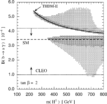
Figure 7: Br($b\rightarrow s\gamma$) in the supergravity model as a function of the charged Higgs boson mass for $\tan{\beta}$=2. The solid line shows the branching ratio in the two Higgs doublet model (Model II). The dark points represent the results for the minimal supergravity and the light points correspond to the extended parameter space where SUSY soft breaking parameters at the GUT scale are different for squark/slepton and Higgs fields. Also the SM prediction and the CLEO 95 bound $\!{}^{{\bf?}}$ are shown.

Since only the coefficient of $O_{7}$ is significantly affected by the SUSY contribution there is a strong correlation between the $b\rightarrow s\gamma$ and $b\rightarrow sl^{+}l^{-}$ branching ratios. Figure 8 shows this correlation for $\tan{\beta}=30$. Here $b\rightarrow s\mu^{+}\mu^{-}$ branching ratio is integrated over lepton invariant spectrum below the $J/\psi$ threshold to avoid the large resonance peak. We can see that there are two fold ambiguity which corresponds to the sign of the coefficient of $O_{7}$. When the SUSY and charged Higgs contribution is (-2) times the SM contribution the $b\rightarrow s\gamma$ branching ratio is the same as the SM while the $b\rightarrow sl^{+}l^{-}$ branching ratio can be enhanced by about a factor of two. In the supergravity model this situation arises only for large $\tan{\beta}$ case. The lepton forward and backward asymmetry can also show sizable deviation from the SM in this case.

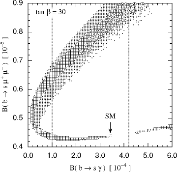
Figure 8: Correlation between Br($b\rightarrow s\gamma$) and Br($b\rightarrow sl^{+}l^{-}$) in the supergravity model for $\tan{\beta}$= 30. Here Br($b\rightarrow s\mu^{+}\mu^{-}$) is obtained by integrating in the range $2m_{\mu}<\sqrt{s}<m_{J/\psi}-100$ MeV where $\sqrt{s}$ is the invariant mass of $\mu^{+}\mu^{-}$ pair. The vertical lines correspond to the CLEO 95 upper and lower bounds.

4.3 $\Delta M_{B}$, $\epsilon_{K}$, $K_{L}\rightarrow\pi^{0}\nu\bar{\nu}$

We have calculated the $\Delta M_{B}$, $\epsilon_{K}$ and branching ratios of $K_{L}\rightarrow\pi^{0}\nu\bar{\nu}$ and $K^{+}\rightarrow\pi^{+}\nu\bar{\nu}$ in the SUSY model based on supergravity$\!{}^{{\bf?}}$. In Figures 9 and 10 we present $\Delta M_{B_{d}}$ and Br($K_{L}\rightarrow\pi^{0}\nu\bar{\nu})$ in the present model normalized by the same quantities calculated in the SM as the function of the $b\rightarrow s\gamma$ branching ratio. Note that these ratios are essentially independent of the CKM parameters because the SUSY and the charged Higgs boson loop contributions have the same dependence on the CKM parameters. Although we only present the results for $\Delta M_{B_{d}}$ and Br($K_{L}\rightarrow\pi^{0}\nu\bar{\nu})$, $\epsilon_{K}$ and Br($K^{+}\rightarrow\pi^{+}\nu\bar{\nu}$) provide the same constraints on the SUSY parameters respectively because these quantities are almost equal if normalized by corresponding quantities in the SM.

From Figures 9 and 10 we can conclude that the $\Delta M_{B_{d}}$ (and $\epsilon_{K}$) can be enhanced by up to 40% and Br($K_{L}\rightarrow\pi^{0}\nu\bar{\nu})$ (and Br($K_{+}\rightarrow\pi^{+}\nu\bar{\nu}$))is suppressed by up to 10% for extended parameter space and the corresponding numbers for the minimal case are 20% and 3%. The ratio of two Higgs vacuum expectation value, $\tan{\beta}$, is 2 for these figures and the deviation from the SM turns out to be smaller for large value of $\tan{\beta}$.

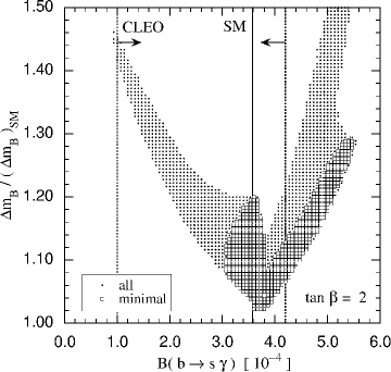
Figure 9: $\Delta M_{B_{d}}$ normalized by the SM value for $\tan{\beta}=2$ as a function of $b\rightarrow s\gamma$ branching ratio. The dark (light) points correspond to the minimal (enlarged) parameter space of the supergravity model. The vertical lines correspond to the CLEO 95 upper and lower bounds.

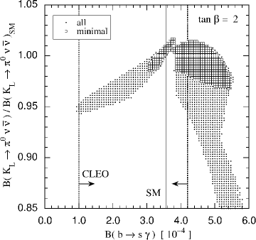
Figure 10: Br($K_{L}\rightarrow\pi^{0}\nu\bar{\nu})$ normalized by the SM value for $\tan{\beta}=2$ as a function of $b\rightarrow s\gamma$ branching ratio.

These deviations may be evident in future when B factory experiments provide additional information on the CKM parameters. It is expected that the one of the three angles of the unitarity triangle is determined well through the $B\rightarrow J/\psi K_{S}$ mode. Then assuming the SM, one more physical observable can determine the CKM parameters or $(\rho,\eta)$ in the Wolfenstein parameterization. New physics effects may appear as inconsistency in the determination of these parameters from different inputs. For example, the $\rho$ and $\eta$ parameters determined from CP asymmetry of B decay in other modes, $\frac{\Delta M_{B_{s}}}{\Delta M_{B_{d}}}$ and $|V_{ub}|$ can be considerably different from those determined through $\Delta M_{B_{d}}$ $\epsilon_{K}$ and Br($K\rightarrow\pi\nu\bar{\nu})$ because $\Delta M_{B_{d}}$ $\epsilon_{K}$ are enhanced and Br($K\rightarrow\pi\nu\bar{\nu})$’s are suppressed in the present model. It turns out that there is strong correlation between deviation of two quantities, namely the latters are most suppressed where the formers have the largest deviation from the SM. The pattern of these deviations from the SM will be a key to distinguish various new physics effects. We also note from Figure 9 and 10 that, although the new results reported at ICHEP98 ($2.0\times 10^{-4}<$Br$(b\rightarrow s\gamma)<4.5\times 10^{-4}$) $\!{}^{{\bf?}}$ does not change the situation very much, future improvement on the $b\rightarrow s\gamma$ branching will give great impacts on constraining the size of possible deviation from the SM in FCNC processes.

5 LFV in the SUSY GUT

5.1 $\mu^{+}\rightarrow e^{+}\gamma$ in SUSY GUT

In the minimal SM with massless neutrinos the lepton number is conserved separately for each generation. This is not necessarily true if we consider physics beyond the SM. LFV can easily occur in many extension of the SM. Experimentally, LFV searches are continued in various processes and especially strong bounds are obtained for muon processes such as $\mu^{+}\rightarrow e^{+}\gamma$, $\mu^{+}\rightarrow e^{+}e^{+}e^{-}$ and $\mu^{-}-e^{-}$ conversion in atoms. The experimental upper bound on these processes quoted in PDG 98 are Br($\mu^{+}\rightarrow e^{+}\gamma$) $\leq 4.9\times 10^{-11}$, Br($\mu^{+}\rightarrow e^{+}e^{+}e^{-}$) $\leq 1.0\times 10^{-12}$ and $\frac{\sigma(\mu^{-}T_{i}\rightarrow e^{-}T_{i})}{\sigma(\mu^{-}T_{i}\rightarrow caputure)}\leq 4.3\times 10^{-12}$. Recently there are considerable interests on these processes because predicted branching ratios turn out to be close to the upper bounds in the SUSY GUT.$\!{}^{{\bf?}}$

As discussed in previous sections no LFV is generated at the Planck scale in the context of the minimal supergravity model. In the SUSY GUT scenario, however, the LFV can be induced through renormalization effects on slepton mass matrix because the GUT interaction breaks lepton flavor conservation. In the minimal SUSY SU(5) GUT, the effect of the large top Yukawa coupling constant results in the LFV in the right-handed slepton sector. This induces $\mu^{-}\rightarrow e^{-}_{R}\gamma$ ($\mu^{+}\rightarrow e^{+}_{L}\gamma$) decay. The branching ratio can be calculated based on this model and it was pointed out that there is unfortunate cancellation between different diagrams so that Br($\mu^{+}\rightarrow e^{+}\gamma$) is below $10^{-13}$ level for most of the parameter space.$\!{}^{{\bf?}}$

In the SO(10) SUSY GUT model, on the other hand, both left- and right-handed sleptons induce LFV because of different structure of Yukawa coupling constants at the GUT scale. More importantly, there are diagrams which enhance the branching ratio by a factor $(\frac{m_{\tau}}{m_{\mu}})^{2}$ compared to the minimal SU(5) SUSY GUT model and predicted branching ratio is at least larger by two order of magnitudes.$\!{}^{{\bf?}}$

A similar enhancement can occur also in the context of the SUSY SU(5) model for large value of $\tan{\beta}$ once we take into account effects of higher dimensional operators to explain realistic fermion masses.$\!{}^{{\bf?}}$ In the minimal case the Yukawa coupling is given by the superpotential $W=(y_{u})_{ij}{\bf T_{i}}\cdot{\bf T_{j}}\cdot{\bf H(5)}+(y_{d})_{ij}{\bf T_{i}}\cdot{\bf\bar{F}_{j}}\cdot{\bf\bar{H}(5)}$ where ${\bf T_{i}}$ is 10 dimensional and ${\bf\bar{F}_{j}}$ is 5 dimensional representation of SU(5). This superpotential alone cannot explain the lepton and quark mass ratios for the first and second generations although the $m_{b}/m_{\tau}$ ratio is in reasonable agreement. One way to obtain realistic mass ratios are to introduce higher dimensional operators such as $\frac{f_{ij}}{M_{Planck}}{\bf\Sigma(24)}\cdot{\bf T_{i}}\cdot{\bf\bar{F}_{j}}\cdot{\bf\bar{H}(5)}$. We investigated how inclusion of these terms changes prediction of the branching ratio. It turns out that the branching ratio is quite sensitive to the details of these higher dimensional operators. Firstly, once we include these terms the slepton mixing matrix elements $\lambda_{\tau}\equiv V_{\tilde{e}31}^{*}V_{\tilde{e}32}$ which appear in the formula of the $\mu^{+}\rightarrow e^{+}\gamma$ amplitude is no longer related to the corresponding CKM matrix elements. More importantly, for large value of $\tan{\beta}$, the left-handed slepton also induces the LFV and the predicted branching ratio becomes enhanced by two order of magnitudes as in the SO(10) case.$\!{}^{{\bf?}}$ The destructive interference among the different diagrams also disappear. We show one example of such calculation in Figure 11 where Br($\mu^{+}\rightarrow e^{+}\gamma$) can be close to $10^{-11}$ level for large values of $\tan{\beta}$ in the non-minimal case.

Figure 11: Dependence of the branching ratio of $\mu\rightarrow e\gamma$ on $\tan\beta$ for the right-handed selectron mass 200GeV (dashed lines) and 300GeV (solid lines). The thick lines are for the non-minimal case that $V_{\bar{e}}$ and $V_{l}$ are the same as $V_{\rm KM}$, and the thin lines are for the minimal case in which $V_{\bar{e}}=V_{\rm KM}$ and $V_{l}={\bf 1}$. In this figure we choose the bino mass 60GeV, the coefficient of the A term $a_{0}$ =0, the higgsino mass positive. The long-dashed line is the experimental upper bound.

Another example of possible large LFV is a SUSY model with the see-saw type neutrino mass.$\!{}^{{\bf?}}$ If we include the right-handed neutrino supermultiplet at high energy scale, we can include large Yukawa coupling constant among lepton doublet, right-handed neutrino and Higgs doublet field. The renormalization effect can induce the LFV in the left-handed slepton sector and in this case $\mu^{-}\rightarrow e^{-}_{L}\gamma$ ($\mu^{+}\rightarrow e^{+}_{R}\gamma$) decay can occur. The branching ratio depends on, among other things, the magnitude of the Yukawa coupling constant which is a function of the neutrino mass and the Majorana mass scale. Therefore even if we fix the neutrino mass motivated by atmospheric and solar neutrino problem the branching ratio strongly depends on the right-handed neutrino mass scale. If the Yukawa coupling constant is assumed to be as large as the top Yukawa coupling constant the predicted the branching ratio can reach the present experimental upper bound. Note that without SUSY neutrino mass can only induce negligible effect to the LFV processes for $\mu$ and $\tau$ decay. It is therefore interesting that the same source of LFV can be responsible for the neutrino oscillation and the $\mu\rightarrow e\gamma$ decay in the SUSY model.

5.2 LFV process with polarized muons

Finally we would like to discuss usefulness of the polarized muons in search for LFV. A highly polarized muon beam is available in $\mu^{+}$ decay experiments. Muons from $\pi^{+}$ decay stopped near the surface of pion production target is 100% polarized opposite to the muon momentum and this muon is called surface muon.

The first obvious merit of polarized muons in $\mu^{+}\rightarrow e^{+}\gamma$ is that we can distinguish $\mu^{+}\rightarrow e^{+}_{R}\gamma$ and $\mu^{+}\rightarrow e^{+}_{L}\gamma$ by the angular distribution of the decay products with respect to the muon polarization direction. For example, the positron from the $\mu^{+}\rightarrow e^{+}_{R}\gamma$ decay follows the $(1-P\cos{\theta})$ distribution where $\theta$ is the angle between the polarization direction and the positron momentum and $P$ is the the muon polarization. In the previous examples the SU(5) SUSY GUT for small $\tan{\beta}$ predicts $\mu^{+}\rightarrow e^{+}_{L}\gamma$ because LFV is induced only in the right-handed slepton sector. On the other hand the SO(10) SUSY GUT generates both $\mu^{+}\rightarrow e^{+}_{L}\gamma$ and $\mu^{+}\rightarrow e^{+}_{R}\gamma$. If LFV is induced by the right-handed neutrino Yukawa coupling constant, only $\mu^{+}\rightarrow e^{+}_{R}\gamma$ should be observed.

Polarized muons are also useful to suppress background processes for the $\mu^{+}\rightarrow e^{+}\gamma$ search.$\!{}^{{\bf?}}$ In this mode the experimental sensitivity is limited by appearance of the background processes. There are two major background processes. The first one is physics background process which is a tail of radiative muon decay. If neutrino pair carries out only little energy in the $\mu^{+}\rightarrow e^{+}\nu\bar{\nu}\gamma$ process, we cannot distinguish this from the signal process. The second background process is an accidental background process where detections of 52.8 MeV positron and 52.8 MeV photon from different muon decays coincide within time and angular resolutions for selection of signals. The source of the 52.8 MeV positron is the ordinary $\mu^{+}\rightarrow e^{+}\nu\bar{\nu}$ decay whereas the 52.8 MeV photon mainly comes from a tail of the radiative muon decay. In the experiment with polarized muons angular distribution is useful to suppress both backgrounds. Suppression of the accidental background turns out to be more important in the next generation experiment. In this case both positrons and photons follow the $(1+P\cos{\theta})$ distribution. Since the signal is back-to-back the background suppression works independently of the signal distribution. If we use 97% polarized muons we can expect to reduce the accidental background by one order of magnitude. This looks promising for search of $\mu^{+}\rightarrow e^{+}\gamma$ at the level of $10^{-14}$ branching ratio.

Figure 12:  T-odd asymmetry ${\bf A}$ as a function of the right-handed selectron mass in $\mu\rightarrow 3e$ precess in the SUSY SU(5) GUT. We fix the SUSY parameters as $M_{2}=200$ GeV, $A_{X}=i$, $\mu>0$ and $\tan\beta=3$ (dotted line), 10 (solid line), 30 (dashed line) and top quark mass as 175 GeV.

Last example of usefulness of polarized muons is that we can measure T violating asymmetry in the $\mu^{+}\rightarrow e^{+}e^{+}e^{-}$ decay. Using polarization of initial muons we can define T odd triple vector correlation $<\vec{P}\cdot(\vec{p_{1}}\times\vec{p_{2}})>$ where $\vec{P}$ is muon polarization and $\vec{p_{1}}$ and $\vec{p_{1}}$ are two independent momenta of decay particles.$\!{}^{{\bf?}}$ We have investigated T odd asymmetry in the SU(5) SUSY GUT.$\!{}^{{\bf?}}$ In order to have this asymmetry we need to introduce a CP violating phase other than the KM phase. This phase can be provided by the complex phases in the SUSY breaking terms, for example, the phase in the triple scalar coupling constant (A term). Since this phase also induces electron and neutron EDMs, we have calculates the T odd asymmetry in the $\mu^{+}\rightarrow e^{+}e^{+}e^{-}$ taking into account EDM constraints. In Figure12 we show one example of such calculation for the T odd asymmetry. By examining SUSY parameter space we found that the asymmetry up to 20% is possible. The branching ratio for $\mu^{+}\rightarrow e^{+}e^{+}e^{-}$ turns out to crucially depend on the slepton mixing element $\lambda_{\tau}$ which is an unknown parameter once we take into account the higher dimensional operators for the Yukawa coupling constants. For $\lambda_{\tau}=10^{-2}$ we can show that the branching ratio of $10^{-14}$ is possible with 10% asymmetry which can be reached in future experiment with sensitivity of $10^{-16}$ level.

6 Conclusions

I have reviewed some aspects of the Higgs physics and flavor physics in SUSY theories. An important feature of SUSY models is existence of light Higgs boson which is a target of LEP II, Tevatron and LHC experiments. I have also shown that a future $e^{+}e^{-}$ linear collider is an ideal place to study the SUSY Higgs sector. At earlier stage of the experiment with $\sqrt{s}\sim$ 300 - 500 GeV, it is easy to find a light Higgs boson predicted in SUSY standard models. In particular, both in the MSSM and the SUSY SM with a gauge singlet Higgs, at least one of neutral Higgs bosons is detectable. More importantly, detailed study on properties of the Higgs boson is possible at an $e^{+}e^{-}$ linear collider through measurements of various production cross-sections and branching ratios. As an example we show that the measurement of Higgs couplings to $c\bar{c}$/$gg$/$b\bar{b}$ gives us important information on the Higgs sector of the MSSM. Combining expected results at LHC we may be able to clarify the Higgs sector of the SM and explore physics beyond the SM such as the SUSY SM in future $e^{+}e^{-}$ linear collider experiments.

We have considered various flavor changing processes in the supersymmetric standard model based on the supergravity. We have seen that the branching ratio of $b\rightarrow s\gamma$ is very sensitive to SUSY effects and further improved measurement of this process is important. Flavor changing neutral current processes in B and K decays such as $B^{0}-\bar{B^{0}}$ mixing, $\epsilon_{K}$ and branching ratio of $K\rightarrow\pi\nu\bar{\nu}$ are calculated and it is shown that the deviation from the SM becomes as large as 40 % for $B^{0}-\bar{B^{0}}$ mixing and $\epsilon_{K}$ but somewhat smaller for $K\rightarrow\pi\nu\bar{\nu}$ processes. We also investigated LFV in the SU(5) SUSY GUT. It is pointed out that the $\mu\rightarrow e\gamma$ branching ratio can be enhanced for large $\tan{\beta}$ if we take into account the higher dimensional operators in the Yukawa coupling constants at the GUT scale. The T odd triple vector correlation is also calculated for the $\mu^{+}\rightarrow e^{+}e^{+}e^{-}$ process and it is shown that the asymmetry up to 20% is possible due to the CP violating phases in the supersymmetry breaking terms. Experiments on B, K and LFV processes in near future, therefore, will provide very important opportunities to investigate into the structure of the SUSY breaking sector.

References

References

- [1] J. Wess and B. Zumino, Nucl. Phys. B 70, 39 (1974); D.V. Volkov and V.P. Akulov, Phys. Lett. B 46, 109 (1973).
- [2] D.F. Freedman, P. van Nieuwenhuizen and S. Ferrara, Phys. Rev. D 13, 3714 (1976).
- [3] F. Gliozzi, J. Scherk and D.I. Olive, Phys. Lett. B 65, 282 (1973); Nucl. Phys. B 122, 253 (1977) .
- [4] For review, see H.P. Nilles, Phys. Rep. 110, 1 (1984).
- [5] P. Langacker and M. Luo,Phys. Rev. D 44, 817 (1991); U. Amaldi, W. de Beor and H. Fürstenau,Phys. Lett. B 260, 447 (1991) .
- [6] For example, J. Wess and J. Bagger Supersymmetry and Supergravity (Princeton University Press, Princeton, 1992).
- [7] L. Girardello and M.T. Grisaru, Nucl. Phys. B 194, 65 (1982).
- [8] S. Ferrara, L. Girardello and F. Palumbo, Phys. Rev. D 20, 403 (1979).
- [9] M. Dine and A. Nelson, Phys. Rev. D 48, 1277 (1993); M. Dine, A. Nelson, and Y. Shirman, Phys. Rev. D 51, 1362 (1995); M. Dine, A. Nelson, Y. Nir, and Y. Shirman, Phys. Rev. D 53, 2658 (1996).
- [10] For example, ALEPH collaboration. Barate et al., Phys. Lett. B 429, 201 (1998); Phys. Lett. B 433, 176 (1998).
- [11] Y. Okada, M. Yamaguchi and T. Yanagida, Prog. Theor. Phys. 85, 1 (1991); J. Ellis, G. Ridolfi and F. Zwirner, Phys. Lett. B 257, 83 (1991); H.E. Haber and R. Hempfling, Phys. Rev. Lett. 66, 1815 (1991).
- [12] Y. Okada, M. Yamaguchi and T. Yanagida, Phys. Lett. B 262, 54 (1991).
- [13] R. Barbieri, M. Frigeni, and F. Caravaglios, Phys. Lett. B 258, 167 (1991).
- [14] M. Drees, Int. J. Mod. Phys. A 4, 3635 (1989) 3635; J. Ellis, J.F. Gunion, H.E. Haber, L. Roszkowski and F. Zwirner, Phys. Rev. D 39, 844 (1989); L. Durand and J.L. Lopez, Phys. Lett. B 217, 463 (1989); J.R. Espinosa and M. Quirós, Phys. Lett. B 279, 92 (1992).
- [15] P.Binétruy and C.A. Savoy, Phys. Lett. B 277, 453 (1992); T. Moroi and Y. Okada, Phys. Lett. B 295, 73 (1992); G. Kane, C. Kolda and J. Wells, Phys. Rev. Lett. 70, 2686 (1993); W.T.A. ter Veldhuis, Purdue preprint, PURD-TH-92-11; J.R. Espinosa and M. Quirós, Phys. Lett. B 302, 51 (1993); U. Ellwanger,Phys. Lett. B 303, 271 (1993); P.N. Pandita,Phys. Lett. B 318, 338 (1993); Z. Phys. C 59, 575 (1993); T. Elliot, S.F. King and P.L. White, Phys. Lett. B 305, 71 (1993); Phys. Rev. D 49, 4435 (1994).
- [16] J. Kamoshita, Y. Okada and M. Tanaka, Phys. Lett. B 328, 67 (1994); S.F. King and P.L. White, Phys. Rev. D 53, 4049 (1996).
- [17] T. Moroi and Y. Okada, Phys. Lett. B 295, 73 (1992).
- [18] J.R. Espinosa and M. Quirós, Phys. Rev. Lett. 81, 516 (1998).
- [19] ATLAS Technical Proposal (1994); CMS Technical Proposal (1994); E. Richter-Was, D. Froidevaux, F. Gianotti, L. Poggioli, D. Cavalli, and S. Resconi, Int.J. Mod. Phys. A 13, 1371 (1998).
- [20] P. Janot in Proceedings of the Workshop on Physics and Experiments with Linear Colliders, Waikola, Hawaii, 1993 edited by F. Harris et al. (World Scientific, Singapore, 1993).
- [21] K. Kawagoe in Proceedings of the Workshop on Physics and Experiments with Linear Colliders, Waikola, Hawaii, 1993 edited by F. Harris et al. (World Scientific, Singapore, 1993).
- [22] JLC-I, KEK Report 92-16, December 1992.
- [23] M.D. Hildreth, T.B. Barklow and D.L. Burke, Phys. Rev. D 49, 3441 (1994).
- [24] J. Kamoshita, Y. Okada and M. Tanaka, in Proceedings of the Workshop on Physics and Experiments with Linear Colliders, Morioka-Appi, Iwate, Japan 1995 edited by A. Miyamoto et al. (World Scientific, Singapore, 1996); Phys. Lett. B 391, 124 (1997).
- [25] I. Nakamura and K. Kawagoe, in Proceedings of the Workshop on Physics and Experiments with Linear Colliders, Morioka-Appi, Iwate, Japan 1995 edited by A. Miyamoto et al. (World Scientific, Singapore, 1996); Phys. Rev. D 54 , 3634 (1996).
- [26] A. Djouadi, M. Spira and P.M. Zerwas, Z. Phys. C 70, 427 (1996).
- [27] S. Bertolini, F. Borzumati, A. Masiero and G. Ridolfi, Nucl. Phys. B 353, 591 (1991).
- [28] T. Goto and Y. Okada, Prog. Theor. Phys. 94, 407 (1995) and references therein.
- [29] A. Ali, G. Giudice and T. Mannel, Z. Phys. C 67, 417 (1995); P. Cho, M. Misiak and D. Wyler, Phys. Rev. D 54, 3329 (1996); T. Goto, Y. Okada, Y. Shimizu and M. Tanaka, Phys. Rev. D 55, 4273 (1997); J. Hewett, J.D. Wells, Phys. Rev. D 55, 5549 (1997).
- [30] T. Goto, T. Nihei and Y. Okada, Phys. Rev. D 53, 5233 (1996); Erratum, ibid. D54, 5904 (1996).
- [31] R. Barbieri and L.J. Hall, Phys. Lett. B 338, 212 (1994).
- [32] T. Goto, Y. Okada, and Y. Shimizu, Phys. Rev. D 58, 094006 (1998).
- [33] J. Ellis, S. Ferrara and D.V. Nanopoulos, Phys. Lett. B 114, 231 (1982); W. Buchmüller and D. Wyler, Phys. Lett. B 121, 321 (1983); J. Polchinski and M. Wise, Phys. Lett. B 125, 393 (1983); F. del Aguila, M. Gavela, J. Grifols and A. Mendez, Phys. Lett. B 126, 71 (1983); D.V. Nanopoulos and M. Srednicki, Phys. Lett. B 128, 61 (1983); M. Dugan, B. Grinstein and L. Hall, Nucl. Phys. B 255, 413 (1985); Y. Kizukuri and N. Oshimo, Phys. Rev. D 45, 1806 (1992); Phys. Rev. D 46, 3025 (1992); T. Falk and K.A. Olive, Phys. Lett. B 375, 196 (1996); T. Ibrahim and P. Nath, Phys. Lett. B 418, 98 (1998); Phys. Rev. D 57, 478 (1998).
- [34] T. Nihei, Prog. Theor. Phys. 98, 1157 (1997).
- [35] CLEO Collaboration, M.S. Alam et al., Phys. Rev. Lett. 74, 2885 (1995).
- [36] CLEO Collaboration, CLEO CONF 98-17.
- [37] J. Hisano, T. Moroi, K. Tobe and M. Yamaguchi, Phys. Lett. B 391, 341 (1997); Erratum, ibid. B 397, 357 (1997).
- [38] R. Barbieri, L. Hall, and A. Strumia, Nucl. Phys. B 445, 219 (1995).
- [39] J. Hisano, D. Nomura, Y. Okada, Y. Shimizu and M. Tanaka, Phys. Rev. D 58, 116010 (1998).
- [40] N. Arkani-Hamed, H. Cheng, and L. Hall, Phys. Rev. D 53, 413 (1996).
- [41] F. Borzumati and A. Masiero, Phys. Rev. Lett. 57, 961 (1986); J. Hisano, T. Moroi, K. Tobe, M. Yamaguchi and T. Yanagida, Phys. Lett. B 357, 579 (1995); J. Hisano, T. Moroi, K. Tobe and M. Yamaguchi, Phys. Rev. D 53, 2442 (1996); J. Hisano, D. Nomura, and T. Yanagida, Phys. Lett. B 437, 351 (1998); J. Hisano and D. Nomura KEK-TH-602, hep-ph/9810479.
- [42] Y. Kuno and Y. Okada Phys. Rev. Lett. 77, 434 (1996); Y. Kuno, A. Maki, and Y. Okada Phys. Rev. D 55, 2517 (1997).
- [43] S.B. Treiman, F. Wilczek and A. Zee, Phys. Rev. D 16, 1977 (152).
- [44] Y. Okada, K. Okumura and Y. Shimizu, Phys. Rev. D 58, 051901 (1998).