hep-ph/9811492

DOE-ER-40757-121

UTEXAS-HEP-98-23

ILL-(TH)-98-5

ANL-HEP-PR-98-138

EFI-98-57

November 1998

Higgs-Boson Production in Association with
Bottom Quarks at Next-to-Leading Order

D. Dicus

Center for Particle Physics

Department of Physics

University of Texas

Austin, TX  78712

T. Stelzer

Department of Physics

University of Illinois

1110 West Green Street

Urbana, IL  61801

Z. Sullivan

High Energy Physics Division

Argonne National Laboratory

Argonne, IL  60439

S. Willenbrock

Enrico Fermi Institute and Department of Physics

University of Chicago

5640 S. Ellis Avenue

Chicago, IL  60637

and

Department of Physics

University of Illinois

1110 West Green Street

Urbana, IL  61801

We argue that the leading-order subprocess for Higgs-boson production in association with bottom quarks is $b\bar{b}\to H$. This process is an important source of Higgs bosons with enhanced Yukawa coupling to bottom quarks. We calculate the corrections to this cross section at next-to-leading-order in $1/\ln(m_{H}/m_{b})$ and $\alpha_{s}$ and at next-to-next-to-leading order in $1/\ln(m_{H}/m_{b})$.

1 Introduction

The standard-model Higgs boson has a very weak Yukawa coupling to bottom quarks, proportional to $m_{b}/v$, where $v\approx 246$ GeV is the vacuum-expectation value of the Higgs field. Therefore, the cross section for the production of the standard-model Higgs boson in association with bottom quarks is relatively small at the Fermilab Tevatron [1] and the CERN Large Hadron Collider (LHC) [2], in comparison with other Higgs-boson production cross sections. However, if the bottom-quark Yukawa coupling is enhanced, this production mechanism can be a significant source of Higgs bosons [2]. Such an enhancement occurs, for example, in a two-Higgs-doublet model for large values of $\tan\beta\equiv v_{2}/v_{1}$, where $v_{1,2}$ are the vacuum-expectation values of the two Higgs fields. A value as large as $\tan\beta\approx m_{t}/m_{b}$ is obtained in the simplest version of an SO(10) grand-unified theory. The Higgs boson may be detected via its decay to $\tau^{+}\tau^{-}$ [3, 4, 5] or $b\bar{b}$ [5, 6, 7, 8] at the LHC and the Tevatron, and $\mu^{+}\mu^{-}$ [9] at the LHC.

In this paper we calculate the cross section for Higgs-boson production in association with bottom quarks at next-to-leading order. We argue that the leading-order subprocess is $b\bar{b}\to H$, where the initial $b$-quark distribution function is calculated [10, 11]. We show that the subprocess $gb\to Hb$ is a correction to the leading-order subprocess of order $1/\ln(m_{H}/m_{b})$, and that the subprocess $gg\to b\bar{b}H$ is a correction of order $1/\ln^{2}(m_{H}/m_{b})$. We calculate both of these corrections, and confirm the calculation performed by two of us ten years ago [2]. Our new contribution to this part of the calculation is a proper understanding of the relative order of the different subprocesses.

Once we properly identify $b\bar{b}\to H$ as the leading-order subprocess, it is straightforward to calculate the order $\alpha_{s}$ correction from the emission of virtual and real gluons. This calculation is performed here for the first time. We thus obtain the cross section for Higgs-boson production in association with bottom quarks at next-to-leading order in both $\alpha_{s}$ and $1/\ln(m_{H}/m_{b})$, as well as at next-to-next-to-leading order in $1/\ln(m_{H}/m_{b})$. Our calculation is valid for both scalar and pseudoscalar Higgs bosons.

Our calculation corresponds to the inclusive cross section for Higgs-boson production in association with bottom quarks, integrated over the momenta of the $b$ quarks. It is appropriate to use our results to normalize the inclusive cross section from a shower Monte Carlo program, such as PYTHIA or HERWIG, which uses $b\bar{b}\to H$ as the hard-scattering subprocess.

The remainder of this paper is organized as follows. In Sec. 2 we explain how to properly count the order of the various contributions to Higgs-boson production in association with heavy quarks. In Sec. 3 we perform the calculation of the $1/\ln(m_{H}/m_{Q})$ and $1/\ln^{2}(m_{H}/m_{Q})$ corrections. In Sec. 4 we calculate the $\alpha_{s}$ correction. In Sec. 5 we present numerical results at the Tevatron and the LHC.

2 Counting orders

2.1 $1/\ln(m_{H}/m_{Q})$ correction

In this section we explain how to count the order of the various contributions to Higgs-boson production in association with heavy quarks. This counting is a generalization, to the case with two heavy quarks in the initial state, of the counting developed in Ref. [12] for a subprocess with one heavy quark in the initial state ($qb\to qt$). The underlying concepts for the organization of the calculation were developed in Refs. [10, 11].

The actual physical subprocess for Higgs-boson production in association with heavy quarks is $gg\to Q\overline{Q}H$, shown in Fig. 1. Imagine that the heavy quark is very light compared with the Higgs-boson. When the initial gluon splits into a nearly-collinear $Q\overline{Q}$ pair, the amplitude is enhanced by the propagator of the internal heavy quark, which is nearly on-shell. Integrating over the phase space of the external heavy quark yields a factor of $\ln(m_{H}/m_{Q})$, so the splitting of a gluon into a $Q\overline{Q}$ pair is intrinsically of order $\alpha_{s}\ln(m_{H}/m_{Q})$ (for $m_{H}\gg m_{Q}$). Such a splitting occurs twice in each of the first two diagrams of Fig. 1, once in each of the next four diagrams, and not at all in the final two diagrams.

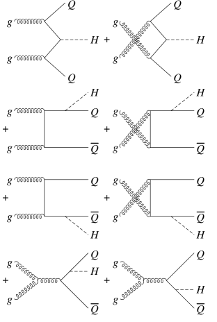
Figure 1: Feynman diagrams for $gg\to Q\overline{Q}H$.

Another power of this logarithm appears at every order in perturbation theory, via the emission of a collinear gluon from the nearly-on-shell quark propagator. Thus the expansion parameter is $\alpha_{s}\ln(m_{H}/m_{Q})$, and since the logarithm is large, the convergence of the expansion is degraded.

The convergence of the expansion is improved by summing these collinear logarithms to all orders in perturbation theory [10, 11]. This is achieved by introducing a (theoretically-defined) heavy-quark distribution function, $Q(x,\mu)$, and using the Dokshitzer-Gribov-Lipatov-Altarelli-Parisi (DGLAP) equations to sum the collinear logarithms. The heavy-quark distribution function is intrinsically of order $\alpha_{s}\ln(m_{H}/m_{Q})$ since it arises from the splitting of a gluon into a nearly-collinear $Q\overline{Q}$ pair [12].

Once a heavy-quark distribution function is introduced, it changes the way perturbation theory is ordered. The leading-order subprocess is $Q\overline{Q}\to H$, as shown in Fig. 2(a). It is intrinsically of order $\alpha_{s}^{2}\ln^{2}(m_{H}/m_{Q})$, since each heavy-quark distribution function is of order $\alpha_{s}\ln(m_{H}/m_{Q})$. (There is also a factor of the heavy-quark Yukawa coupling, which we suppress throughout this discussion.)

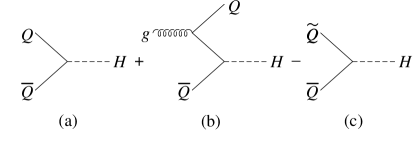
Figure 2: Feynman diagrams for (a) the leading-order subprocess $Q\overline{Q}\to H$; (b) $g\overline{Q}\to H\overline{Q}$ (there is also an $s$-channel diagram, not shown); and (c) $\widetilde{Q}\overline{Q}\to H$, where the heavy-quark distribution function $\widetilde{Q}$ is given by the perturbative solution to the DGLAP equations. Figs. (b) and (c) together constitute the $1/\ln(m_{H}/m_{Q})$ correction to the leading-order subprocess in (a).

Consider next the subprocess $g\overline{Q}\to H\overline{Q}$ (and related subprocesses), shown in Fig. 2(b). This subprocess gives rise to a factor of $\ln(m_{H}/m_{Q})$ from the region where the gluon splits into a nearly-collinear $Q\overline{Q}$ pair. However, this logarithm has been summed into the heavy-quark distribution function in Fig. 2(a), so it must be removed. This is achieved by subtracting the diagram in Fig. 2(c), which corresponds to the subprocess $Q\overline{Q}\to H$, but with the heavy-quark distribution function given by the perturbative solution to the DGLAP equation for a gluon splitting to a $Q\overline{Q}$ pair,

$$\widetilde{Q}(x,\mu)=\frac{\alpha_{s}(\mu)}{2\pi}\ln\left(\frac{\mu^{2}}{m_{Q}^{2}}\right)\int_{x}^{1}\frac{dy}{y}P_{qg}\left(\frac{x}{y}\right)g(y,\mu)\;,$$ (1)

where $g$ is the gluon distribution function, and the DGLAP splitting function is given by

$$P_{qg}(z)=\frac{1}{2}[z^{2}+(1-z)^{2}]\;.$$ (2)

After the cancellation of the logarithm, the sum of the subprocesses in Figs. 2(b) and (c) is of order $\alpha_{s}$ times the order of the other heavy-quark distribution function, i.e., of order $\alpha_{s}^{2}\ln(m_{H}/m_{Q})$. This is down by one power of $\ln(m_{H}/m_{Q})$ with respect to the leading-order subprocess, Fig. 2(a), so it is a correction of order $1/\ln(m_{H}/m_{Q})$.

Now consider the subprocess $gg\to Q\overline{Q}H$, shown in Fig. 3(a). This subprocess gives rise to a factor of $\ln(m_{H}/m_{Q})$ when either gluon splits into a nearly-collinear $Q\overline{Q}$ pair. Since these collinear logarithms have been summed into the heavy-quark distribution functions, they must be subtracted. This is shown in Figs. 3(b)–3(d): each of the two collinear regions must be subtracted, but we must also add back the double-collinear region [Fig. 3(d)], which is subtracted twice [Figs. 3(b) and (c)]. Once the logarithms have been cancelled, the sum of the subprocesses in Fig. 3 is of order $\alpha_{s}^{2}$. This is down by two powers of $\ln(m_{H}/m_{Q})$ with respect to the leading-order subprocess, Fig. 2(a), so it is a correction of order $1/\ln^{2}(m_{H}/m_{Q})$.

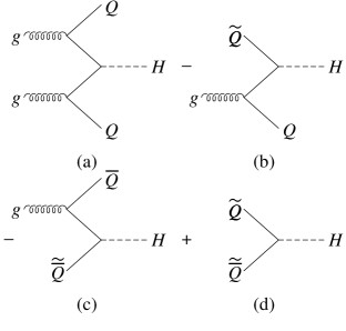
Figure 3: Feynman diagrams for (a) $gg\to Q\overline{Q}H$ (the complete set of diagrams is shown in Fig. 1); (b),(c) $\widetilde{Q}g\to QH$ and $g\widetilde{\overline{Q}}\to H\overline{Q}$ (there are also $s$-channel diagrams, not shown); and (d) $\widetilde{Q}\widetilde{\overline{Q}}\to H$, where the heavy-quark distribution function $\widetilde{Q}$ is given by the perturbative solution to the DGLAP equations. These diagrams together constitute the $1/\ln^{2}(m_{H}/m_{Q})$ correction to the leading-order subprocess $Q\overline{Q}\to H$.

Thus we see that Higgs-boson production in association with heavy quarks contains terms of relative order unity, $1/\ln(m_{H}/m_{Q})$, and $1/\ln^{2}(m_{H}/m_{Q})$, depending on whether the initial state contains two, one, or zero heavy quarks, respectively. These are the only powers of $1/\ln(m_{H}/m_{Q})$ that appear, to all orders in perturbation theory [12].

2.2 $\alpha_{s}$ correction

Now consider the correction to the leading-order subprocess, $Q\overline{Q}\to H$ [Fig. 2(a)], from virtual- and real-gluon emission, shown in Fig. 4. Since these diagrams contain two heavy quarks in the initial state, they are of order $\alpha_{s}^{3}\ln^{2}(m_{H}/m_{Q})$, i.e., down by one power of $\alpha_{s}$ from the leading-order subprocess.

Figure 4: Feynman diagrams for (a) the virtual-gluon correction to $Q\overline{Q}\to H$; (b) $Q\overline{Q}\to Hg$; and (c) $\widetilde{Q}\overline{Q}\to H$, where the heavy-quark distribution function $\widetilde{Q}$ is given by the perturbative solution to the DGLAP equations. These diagrams together constitute the $\alpha_{s}$ correction to the leading-order subprocess $Q\overline{Q}\to H$.

There is a factor of $\ln(m_{H}/m_{Q})$ associated with the emission of a collinear gluon from a heavy quark [Fig. 4(b)], and this is handled in a similar manner to the collinear logarithm associated with a gluon splitting to a $Q\overline{Q}$ pair. The collinear logarithm is summed, to all orders in perturbation theory, into the heavy-quark distribution function, and the collinear region is then explicitly removed by subtracting the subprocess $Q\overline{Q}\to H$ [Fig. 4(c)], with the heavy-quark distribution function given by the perturbative solution to the DGLAP equation for a gluon radiated from a heavy quark. After the cancellation of the collinear logarithms, the sum of Figs. 4(b) and (c) [as well as Fig. 4(a)] is a correction of order $\alpha_{s}$ to the leading-order subprocess $Q\overline{Q}\to H$.

3 The $1/\ln(m_{H}/m_{Q})$ correction

The leading-order hadronic cross section for Higgs-boson production in association with heavy quarks, the $1/\ln(m_{H}/m_{Q})$ correction, and the $1/\ln^{2}(m_{H}/m_{Q})$ correction are obtained from the equations

$$\sigma_{LO} = Q\otimes\sigma^{0}_{Q\overline{Q}\to H}\otimes\overline{Q}+\overline{Q}\otimes\sigma^{0}_{\overline{Q}Q\to H}\otimes Q$$ (3)

$$\sigma_{1/\ln(m_{H}/m_{Q})} = g\otimes\sigma^{1}_{gQ\to HQ}\otimes Q-\widetilde{\overline{Q}}\otimes\sigma^{0}_{\overline{Q}Q\to H}\otimes Q$$ (4)

$$+ Q\otimes\sigma^{1}_{Qg\to QH}\otimes g-Q\otimes\sigma^{0}_{Q\overline{Q}\to H}\otimes\widetilde{\overline{Q}}$$

$$+ g\otimes\sigma^{1}_{g\overline{Q}\to H\overline{Q}}\otimes\overline{Q}-\widetilde{Q}\otimes\sigma^{0}_{Q\overline{Q}\to H}\otimes\overline{Q}$$

$$+ \overline{Q}\otimes\sigma^{1}_{\overline{Q}g\to\overline{Q}H}\otimes g-\overline{Q}\otimes\sigma^{0}_{\overline{Q}Q\to H}\otimes\widetilde{Q}$$

$$\sigma_{1/\ln^{2}(m_{H}/m_{Q})} = g\otimes\sigma^{2}_{gg\to Q\overline{Q}H}\otimes g$$ (5)

$$- \widetilde{Q}\otimes\sigma^{1}_{Qg\to QH}\otimes g-g\otimes\sigma^{1}_{gQ\to HQ}\otimes\widetilde{Q}$$

$$- \widetilde{\overline{Q}}\otimes\sigma^{1}_{\overline{Q}g\to\overline{Q}H}\otimes g-g\otimes\sigma^{1}_{g\overline{Q}\to H\overline{Q}}\otimes\widetilde{\overline{Q}}$$

$$+ \widetilde{Q}\otimes\sigma^{0}_{Q\overline{Q}\to H}\otimes\widetilde{\overline{Q}}+\widetilde{\overline{Q}}\otimes\sigma^{0}_{\overline{Q}Q\to H}\otimes\widetilde{Q}$$

where $Q$ is the heavy-quark distribution function, $\widetilde{Q}$ is the perturbative heavy-quark distribution function [Eq. (1)], $g$ is the gluon distribution function, and they are convolved with the various subprocess cross sections in the usual way. (The parton distribution function written before the subprocess cross section is from hadron A, the one written after from hadron B, and the superscripts on the subprocess cross sections denote the power of $\alpha_{s}$.) This formula implements the discussion in Sec. 2 on the proper way to count the order of the contributions to Higgs-boson production in association with heavy quarks. One can check that the sum of these equations is equivalent to Eq. (5) of Ref. [2], although the proper way to count orders was not known at that time.

For the calculation of the $1/\ln(m_{H}/m_{Q})$ correction (and also the $\alpha_{s}$ correction), it is more convenient to regulate the collinear divergence with dimensional regularization [11] rather than with a finite heavy-quark mass [10]. The former is accurate up to powers of $m_{Q}^{2}/m_{H}^{2}$, which is small in the region of validity of our calculation, $m_{Q}\ll m_{H}$. We perform the calculation of the $1/\ln(m_{H}/m_{Q})$ correction both ways, analytically in the case of dimensional regularization and numerically in the case of a finite heavy-quark mass, and find agreement. The calculation of the $1/\ln^{2}(m_{H}/m_{Q})$ correction is only done numerically, using a finite heavy-quark mass.

We now describe the analytic calculation of the $1/\ln(m_{H}/m_{Q})$ correction using dimensional regularization. The calculation is similar to the QCD correction to the Drell-Yan process from initial gluons [13], but with the vector current replaced by a scalar current.

The spin- and color-averaged cross section for the leading-order subprocess $Q\overline{Q}\to H$ is

$$\sigma^{0}_{Q\overline{Q}\to H}=\frac{\pi}{6}\frac{\overline{m}^{2}(\mu)}{v^{2}}\mu^{2\epsilon}\frac{1}{m_{H}^{2}}\delta(1-z)\;,$$ (6)

where $z\equiv m_{H}^{2}/\hat{s}$. The calculation is performed in $N=4-2\epsilon$ dimensions; $\mu$ is the ‘t Hooft mass, which is introduced such that the renormalized Yukawa coupling is dimensionless in $N$ dimensions. We use the $\overline{\rm MS}$ scheme to subtract ultraviolet (and collinear) divergences, so $\overline{m}(\mu)$ is the heavy-quark $\overline{\rm MS}$ mass.

The spin- and color-averaged cross section for the subprocess $gQ\to HQ$ is

$$\sigma^{1}_{gQ\to HQ}=\frac{\alpha_{s}}{12}\frac{\overline{m}^{2}(\mu)}{v^{2}}\mu^{4\epsilon}\frac{1}{\hat{s}}\Biggl{\{}P_{qg}(z)\Biggl{[}-\frac{1}{\epsilon}\frac{\Gamma(1-\epsilon)}{\Gamma(1-2\epsilon)}+\ln\Biggl{(}\frac{m_{H}^{2}}{4\pi}\frac{(1-z)^{2}}{z}\Biggr{)}\Biggr{]}+\frac{1}{4}(1-z)(7z-3)\Biggr{\}}\;,$$ (7)

where $z\equiv m_{H}^{2}/\hat{s}$. The collinear divergence manifests itself as a pole at $\epsilon=0$. The ‘t Hooft mass accompanies both the renormalized strong coupling and Yukawa coupling, which are defined to be dimensionless in $N$ dimensions.

The perturbative heavy-quark distribution function that subtracts the collinear region in dimensional regularization is

$$\widetilde{Q}(x,\mu)=-\frac{\alpha_{s}}{2\pi}\int_{x}^{1}\frac{dy}{y}P_{qg}\left(\frac{x}{y}\right)g(y,\mu)\left(\frac{1}{\epsilon}-\gamma+\ln 4\pi\right)\;.$$ (8)

This is the analogue of Eq. (1), in which the collinear divergence is regularized by a finite heavy-quark mass. Either distribution function can be used in Eq. (4), and both yield the cross section in the $\overline{\rm MS}$ scheme. Using dimensional regularization, the first line of Eq. (4) yields the cross section

$$\bar{\sigma}_{gQ\to HQ}^{1}=\frac{\alpha_{s}}{12}\frac{\overline{m}^{2}(\mu)}{v^{2}}\frac{1}{\hat{s}}\left[P_{qg}(z)\ln\left(\frac{m_{H}^{2}}{\mu^{2}}\frac{(1-z)^{2}}{z}\right)+\frac{1}{4}(1-z)(7z-3)\right]\;.$$ (9)

This is just Eq. (7) with the term proportional to $(1/\epsilon-\gamma+\ln 4\pi)$ removed by renormalization, and the limit $\epsilon\to 0$ taken. The remaining terms in the $1/\ln(m_{H}/m_{Q})$ correction [lines 2–4 of Eq. (4)] yield the same expression.

The $1/\ln^{2}(m_{H}/m_{Q})$ correction, Eq. (5), can also be calculated analytically using dimensional regularization. However, we find it simpler to perform the calculation numerically, using a finite heavy-quark mass. The perturbative heavy-quark distribution function that subtracts the collinear region is given by Eq. (1), and $m_{Q}$ is kept finite throughout the calculation.

4 The $\alpha_{s}$ correction

The calculation of the $\alpha_{s}$ correction to $Q\overline{Q}\to H$ is also similar to the correction to the Drell-Yan process [13, 14]. However, there is an additional feature: the ultraviolet renormalization of the Yukawa coupling [15]. The electroweak coupling is not renormalized in the Drell-Yan process due to a Ward identity which cancels the ultraviolet divergence.

The interference of the one-loop vertex correction in Fig. 4(a) with the tree diagram in Fig. 2(a) yields the spin- and color-averaged cross section

$$\sigma^{1}_{Q\overline{Q}\to H}=\frac{\pi}{6}\frac{\overline{m}^{2}(\mu)}{v^{2}}\mu^{2\epsilon}\frac{1}{\hat{s}}\delta(1-z)\left[1+C_{F}\frac{\alpha_{s}}{2\pi}\mu^{2\epsilon}\left(\frac{4\pi}{m_{H}^{2}}\right)^{\epsilon}\frac{\Gamma(1-\epsilon)}{\Gamma(1-2\epsilon)}\left(-\frac{2}{\epsilon^{2}}-\frac{3}{\epsilon}-2+\frac{2\pi^{2}}{3}\right)\right]\;,$$ (10)

($C_{F}\equiv 4/3$) which includes both the leading-order and next-to-leading-order terms. The Yukawa coupling has been renormalized in the $\overline{\rm MS}$ scheme, which yields the counterterm [15]

$${\cal L}=-\mu^{\epsilon}\frac{\overline{m}(\mu)}{v}\left(1-\frac{\delta\overline{m}}{\overline{m}}\right)Q\overline{Q}H\;,$$ (11)

where

$$\frac{\delta\overline{m}}{\overline{m}}=C_{F}\frac{\alpha_{s}}{4\pi}3\left(\frac{1}{\epsilon}-\gamma+\ln 4\pi\right)\;.$$ (12)

The cross section displays both a collinear ($1/\epsilon$) and an infrared ($1/\epsilon^{2}$) divergence.

The emission of a real gluon ($Q\overline{Q}\to Hg$) yields the spin- and color-averaged cross section

$$\sigma^{1}_{Q\overline{Q}\to Hg} = C_{F}\frac{\alpha_{s}}{12}\mu^{2\epsilon}\frac{\overline{m}^{2}(\mu)}{v^{2}}\frac{1}{\hat{s}}\left(\frac{4\pi}{m_{H}^{2}}\right)^{\epsilon}\frac{\Gamma(1-\epsilon)}{\Gamma(1-2\epsilon)}$$

$$\times \left[\frac{2}{\epsilon^{2}}\delta(1-z)-\frac{2}{\epsilon}\frac{1+z^{2}}{(1-z)_{+}}-2(1+z^{2})\frac{\ln z}{1-z}+4(1+z^{2})\left(\frac{\ln(1-z)}{1-z}\right)_{+}+2(1-z)\right]\;,$$

where $z\equiv m_{H}^{2}/\hat{s}$, and the “plus” prescription is defined as usual:

$$\int_{0}^{1}dz\,[f(z)]_{+}h(z)\equiv\int_{0}^{1}dz\,f(z)[h(z)-h(1)]\;.$$ (14)

When combined with the cross section from virtual-gluon emission, Eq. (10), the infrared divergences cancel. The collinear divergence is subtracted by constructing the combination

$$\sigma_{\alpha_{s}} = Q\otimes\sigma^{1}_{Q\overline{Q}\to H}\otimes\overline{Q}+\overline{Q}\otimes\sigma^{1}_{\overline{Q}Q\to H}\otimes Q$$ (15)

$$+ Q\otimes\sigma^{1}_{Q\overline{Q}\to Hg}\otimes\overline{Q}-\widetilde{Q}\otimes\sigma^{0}_{Q\overline{Q}\to H}\otimes\overline{Q}-Q\otimes\sigma^{0}_{Q\overline{Q}\to H}\otimes\widetilde{\overline{Q}}$$

$$+ \overline{Q}\otimes\sigma^{1}_{\overline{Q}Q\to Hg}\otimes Q-\widetilde{\overline{Q}}\otimes\sigma^{0}_{\overline{Q}Q\to H}\otimes Q-\overline{Q}\otimes\sigma^{0}_{\overline{Q}Q\to H}\otimes\widetilde{Q}\;,$$

which is the analogue, for virtual- and real-gluon emission, of Eq. (4). The perturbative heavy-quark distribution function in Eq. (15) is given by

$$\widetilde{Q}(x,\mu)=-\frac{\alpha_{s}}{2\pi}\int_{x}^{1}\frac{dy}{y}P_{qq}\left(\frac{x}{y}\right)Q(y,\mu)\left(\frac{1}{\epsilon}-\gamma+\ln 4\pi\right)\;,$$ (16)

where

$$P_{qq}(z)=C_{F}\left(\frac{1+z^{2}}{(1-z)_{+}}+\frac{3}{2}\delta(1-z)\right)\;,$$ (17)

is the DGLAP splitting function for a quark radiating a gluon. The sum of virtual- and real-gluon emission, after the subtraction of the collinear divergence, is

$$\bar{\sigma}^{1}_{Q\overline{Q}\to H}+\bar{\sigma}^{1}_{Q\overline{Q}\to Hg} = \frac{\pi}{6}\frac{\overline{m}^{2}(\mu)}{v^{2}}\frac{1}{\hat{s}}$$ (18)

$$\times \Biggl{\{}\delta(1-z)+\frac{\alpha_{s}}{\pi}P_{qq}(z)\ln\frac{m_{H}^{2}}{\mu^{2}}$$

$$+C_{F}\frac{\alpha_{s}}{2\pi}\Biggl{[}\Biggl{(}-2+\frac{2\pi^{2}}{3}-3\ln\frac{m_{H}^{2}}{\mu^{2}}\Biggr{)}\delta(1-z)$$

$$-2(1+z^{2})\frac{\ln z}{1-z}+4(1+z^{2})\Biggl{(}\frac{\ln(1-z)}{1-z}\Biggr{)}_{+}+2(1-z)\Biggr{]}\Biggr{\}}\;,$$

which is the sum of Eqs. (10) and (LABEL:R), with the term proportional to $(1/\epsilon-\gamma+\ln 4\pi)$ removed by renormalization, and the limit $\epsilon\to 0$ taken.

Since the derivation of Eq. (18) involves the removal of both collinear and ultraviolet divergences, there are actually two independent scales ($\mu$) present. To make this explicit, consider the leading-order running of the heavy-quark mass and the strong coupling [15]:

$$\overline{m}(\mu)=\overline{m}(\mu_{0})\left(\frac{\alpha_{s}(\mu)}{\alpha_{s}(\mu_{0})}\right)^{\frac{1}{\beta_{0}}}\;,$$ (19)

$$\alpha_{s}(\mu)=\frac{\alpha_{s}(\mu_{0})}{1+\beta_{0}[\alpha_{s}(\mu_{0})/\pi]\ln(\mu^{2}/\mu_{0}^{2})}\;,$$ (20)

where $\beta_{0}=(11-2N_{f}/3)/4$ (see the Appendix for the next-to-leading-order equation). The perturbative expansion of Eq. (19) at next-to-leading order is

$$\overline{m}(\mu)=\overline{m}(\mu_{0})\left[1-C_{F}\frac{\alpha_{s}}{4\pi}3\ln\left(\frac{\mu^{2}}{\mu_{0}^{2}}\right)\right]\;.$$ (21)

Using Eq. (21) to replace $\overline{m}(\mu)$ with $\overline{m}(\mu_{UV})$ in Eq. (18) yields our final expression for the correction from virtual- and real-gluon emission,

$$\bar{\sigma}^{1}_{Q\overline{Q}\to H}+\bar{\sigma}^{1}_{Q\overline{Q}\to Hg} = \frac{\pi}{6}\frac{\overline{m}^{2}(\mu_{UV})}{v^{2}}\frac{1}{\hat{s}}$$ (22)

$$\times \Biggl{\{}\delta(1-z)+\frac{\alpha_{s}}{\pi}P_{qq}(z)\ln\frac{m_{H}^{2}}{\mu^{2}}$$

$$+C_{F}\frac{\alpha_{s}}{2\pi}\Biggl{[}\Biggl{(}-2+\frac{2\pi^{2}}{3}-3\ln\frac{m_{H}^{2}}{\mu_{UV}^{2}}\Biggr{)}\delta(1-z)$$

$$-2(1+z^{2})\frac{\ln z}{1-z}+4(1+z^{2})\left(\frac{\ln(1-z)}{1-z}\right)_{+}+2(1-z)\Biggr{]}\Biggr{\}}\;,$$

where we now distinguish between the renormalization scale ($\mu_{UV}$), associated with the running coupling, and the factorization scale ($\mu$), associated with the parton distribution functions.

5 Results and Conclusions

Our numerical results for Higgs-boson production in association with bottom quarks at the Tevatron ($\sqrt{S}=1.8$ and 2 TeV $p\bar{p}$) and the LHC ($\sqrt{S}=14$ TeV $pp$) are presented in Table 1. All cross sections are evaluated with the CTEQ4M parton distribution functions [16]. The factorization ($\mu$) and renormalization ($\mu_{UV}$) scales are both set equal to $m_{H}$. The running $b$ mass is evolved from an initial value of $\overline{m}_{b}(M_{b})=4.25\pm 0.15$ GeV [17] using next-to-leading-order evolution equations (see the Appendix) [18]. The value of the running $b$ mass at various values of $\mu_{UV}$ are listed in Table 2. Using $\overline{m}_{b}(m_{H})$, rather than $\overline{m}_{b}(M_{b})$ or $M_{b}$, to evaluate the Yukawa coupling decreases the cross section by about $50\%$. We use the standard-model Yukawa coupling, with no enhancement factor, throughout. Although there is a lower bound of about 70 GeV on the mass of supersymmetric Higgs bosons [19], there is no strict lower bound on the mass of Higgs bosons in a general two-Higgs-doublet model [19, 20], so we include the results for a few smaller masses.

We show the percentage change in the cross section from the corrections of order $1/\ln(m_{H}/m_{b})$, $1/\ln^{2}(m_{H}/m_{b})$, and $\alpha_{s}$, as a function of the Higgs-boson mass, in Figs. 5 (Tevatron) and 6 (LHC). We find that the $1/\ln(m_{H}/m_{b})$ correction is significant and negative at the Tevatron (LHC), ranging from $-94\%$ ($-86\%$) for $m_{H}=40$ GeV to $-35\%$ ($-36\%$) for $m_{H}=1000$ GeV. The size of this correction is a measure of the validity of our calculation; as it approaches approximately $-100\%$, it is no longer justified to regard $b\bar{b}\to H$ as the leading-order subprocess. Our calculation is increasingly justified as one increases the Higgs mass, but the $1/\ln(m_{H}/m_{b})$ correction is significant even for $m_{H}=1000$ GeV.

Figure 5: Percentage change in the cross section for Higgs-boson production in association with bottom quarks from the corrections of order $1/\ln(m_{H}/m_{b})$, $1/\ln^{2}(m_{H}/m_{b})$, and $\alpha_{s}$, as a function of the Higgs-boson mass, at the Tevatron. The next-to-leading-order (NLO) cross section is the sum of the leading-order cross section and the corrections of order $1/\ln(m_{H}/m_{b})$ and $\alpha_{s}$.

Figure 6: Same as Fig. 5, but at the LHC.

The $\alpha_{s}$ correction is also significant, and happens to be positive, such that it largely cancels the $1/\ln(m_{H}/m_{b})$ correction. The $\alpha_{s}$ correction ranges from $+56\%$ for $m_{H}=40$ GeV to $+78\%$ for $m_{H}=1000$ GeV at the Tevatron. The correction increases as the Higgs-boson mass approaches the machine energy due to the presence of a large Sudakov logarithm [21]. Such an effect is not present at the much higher-energy LHC, where the correction ranges from $+52\%$ for $m_{H}=40$ GeV to $+42\%$ for $m_{H}=1000$ GeV.

The $1/\ln^{2}(m_{H}/m_{b})$ correction is modest, ranging from $+20\%$ ($+17\%$) for $m_{H}=40$ GeV to $+3\%$ ($+4\%$) for $m_{H}=1000$ GeV at the Tevatron (LHC). This supports our counting of the order of the various corrections. Since we have not calculated the other next-to-next-to-leading-order corrections, of order $\alpha_{s}^{2}$ and $\alpha_{s}\times 1/\ln(m_{H}/m_{b})$, we do not include the $1/\ln^{2}(m_{H}/m_{b})$ correction in our final result, given in Table 1.

The largest uncertainty in the cross section comes from varying the factorization scale, $\mu$. We show in Figs. 7 (Tevatron) and 8 (LHC) the percentage change in the cross section from its central value ($\mu=m_{H}$) due to varying $\mu$ between $m_{H}/2$ and $2m_{H}$, while keeping $\mu_{UV}=m_{H}$ fixed. The scale variation is generally larger at next-to-leading order than it is at leading order, which indicates that the leading-order scale variation is not a reliable estimate of the uncertainty. The next-to-leading-order uncertainty ranges from about $\pm 30\%$ for $m_{H}=100$ GeV to about $\pm 8.5\%$ ($\pm 13\%$) for $m_{H}=1000$ GeV at the Tevatron (LHC).

Figure 7: Uncertainty in the cross section for Higgs-boson production in association with bottom quarks at the Tevatron, obtained by varying the factorization scale $\mu$ about its central value, $\mu=m_{H}$, from $m_{H}/2$ to $2m_{H}$.

Figure 8: Same as Fig. 7, but at the LHC.

There is a much smaller uncertainty in the cross section from varying the renormalization scale, $\mu_{UV}$, between $m_{H}/2$ and $2m_{H}$. The next-to-leading-order uncertainty ranges from about $\pm 2.5\%$ for $m_{H}=100$ GeV to about $\pm 6\%$ ($\pm 4\%$) for $m_{H}=1000$ GeV at the Tevatron (LHC). This is significantly less than the leading-order uncertainty of about $\pm 11\%$ at both machines. There is also an uncertainty in the cross section of about $\pm 8\%$ from the uncertainty in the $b$-quark mass.

Since the $b$-quark distribution function arises from the gluon distribution function, an additional source of uncertainty is from the gluon-gluon luminosity, which depends on $\tau\approx m_{H}^{2}/S$ [22]. We use the uncertainty advocated in Ref. [22]: $\pm 10\%$ ($\sqrt{\tau}<0.1$); $\pm 20\%$ ($0.1<\sqrt{\tau}<0.2$); $\pm 30\%$ ($0.2<\sqrt{\tau}<0.3$); $\pm 60\%$ ($0.3<\sqrt{\tau}<0.4$). We combine all four sources of uncertainty discussed above in quadrature, and report the uncertainty in the next-to-leading-order cross sections in Table 1.

Our calculation might also be applied to Higgs-boson production in association with top quarks [2, 23, 24]. However, it is only valid for $m_{H}\gg m_{t}$, where $t\bar{t}\to H$ can be regarded as leading order and $gt\to Ht$ can be regarded as a small correction of order $1/\ln(m_{H}/m_{t})$. For $m_{H}\sim m_{t}$, one must regard $gg\to t\bar{t}H$ as the leading-order subprocess (along with $q\bar{q}\to t\bar{t}H$). The $\alpha_{s}$ correction to these subprocesses has not yet been calculated.

In summary, we have calculated the cross section for Higgs-boson production in association with bottom quarks at next-to-leading-order in $1/\ln(m_{H}/m_{b})$ and $\alpha_{s}$, and at next-to-next-to-leading order in $1/\ln(m_{H}/m_{b})$. The most important effect of the next-to-leading-order corrections is taken into account by evaluating the bottom-quark Yukawa coupling using the $\overline{\rm MS}$ mass evaluated at the Higgs mass. The $1/\ln(m_{H}/m_{b})$ and $\alpha_{s}$ corrections are both large, but have the opposite sign, such that the total next-to-leading-order correction is relatively modest.

Table 1: Leading-order and next-to-leading-order cross sections (pb) for Higgs-boson production in association with bottom quarks at the Tevatron ($\sqrt{S}=$ 1.8 and 2 TeV $p\bar{p}$) and the LHC ($\sqrt{S}=$ 14 TeV $pp$). The next-to-leading-order (NLO) cross section is the sum of the leading-order cross section and the corrections of order $1/\ln(m_{H}/m_{b})$ and $\alpha_{s}$. All calculations are performed in the $\overline{\rm MS}$ scheme using CTEQ4M parton distribution functions with $\mu=\mu_{UV}=m_{H}$. The method to obtain the uncertainty in the next-to-leading-order cross section is described in the text.

	$\sqrt{S}=1.8$ TeV $p\bar{p}$			$\sqrt{S}=2$ TeV $p\bar{p}$			$\sqrt{S}=14$ TeV $pp$
$m_{H}$ (GeV)	LO	NLO	(pb)	LO	NLO	(pb)	LO	NLO	(pb)
40	12.30	$7.45\pm 4.17$	$\times 10^{-1}$	15.10	$9.36\pm 5.19$	$\times 10^{-1}$	3.16	$2.10\pm 1.03$	$\times 10^{1}$
60	2.71	$1.99\pm 0.85$	$\times 10^{-1}$	3.41	$2.50\pm 1.07$	$\times 10^{-1}$	9.94	$7.52\pm 2.98$	$\times 10^{0}$
80	8.23	$6.52\pm 2.41$	$\times 10^{-2}$	10.70	$8.52\pm 3.13$	$\times 10^{-2}$	4.12	$3.33\pm 1.16$	$\times 10^{0}$
100	3.05	$2.56\pm 0.86$	$\times 10^{-2}$	4.05	$3.38\pm 1.12$	$\times 10^{-2}$	2.01	$1.69\pm 0.54$	$\times 10^{0}$
120	1.28	$1.11\pm 0.35$	$\times 10^{-2}$	1.74	$1.51\pm 0.47$	$\times 10^{-2}$	11.00	$9.55\pm 2.92$	$\times 10^{-1}$
140	5.90	$5.28\pm 1.57$	$\times 10^{-3}$	8.22	$7.33\pm 2.17$	$\times 10^{-3}$	6.47	$5.76\pm 1.68$	$\times 10^{-1}$
160	2.91	$2.67\pm 0.75$	$\times 10^{-3}$	4.15	$3.79\pm 1.07$	$\times 10^{-3}$	4.02	$3.61\pm 1.01$	$\times 10^{-1}$
180	1.51	$1.42\pm 0.39$	$\times 10^{-3}$	2.21	$2.06\pm 0.56$	$\times 10^{-3}$	2.63	$2.39\pm 0.65$	$\times 10^{-1}$
200	8.21	$7.83\pm 2.49$	$\times 10^{-4}$	1.23	$1.17\pm 0.31$	$\times 10^{-3}$	1.78	$1.65\pm 0.43$	$\times 10^{-1}$
250	2.04	$2.03\pm 0.61$	$\times 10^{-4}$	3.24	$3.19\pm 0.97$	$\times 10^{-4}$	7.66	$7.23\pm 1.79$	$\times 10^{-2}$
300	5.84	$6.01\pm 1.75$	$\times 10^{-5}$	0.98	$1.00\pm 0.29$	$\times 10^{-4}$	3.74	$3.58\pm 0.85$	$\times 10^{-2}$
400	6.10	$6.67\pm 2.36$	$\times 10^{-6}$	1.17	$1.25\pm 0.35$	$\times 10^{-5}$	1.15	$1.14\pm 0.26$	$\times 10^{-2}$
500	7.70	$8.86\pm 3.05$	$\times 10^{-7}$	1.70	$1.93\pm 0.67$	$\times 10^{-6}$	4.34	$4.34\pm 0.92$	$\times 10^{-3}$
600	1.07	$1.29\pm 0.80$	$\times 10^{-7}$	2.75	$3.25\pm 1.10$	$\times 10^{-7}$	1.90	$1.93\pm 0.40$	$\times 10^{-3}$
700	1.54	$1.97\pm 1.21$	$\times 10^{-8}$	4.72	$5.83\pm 3.60$	$\times 10^{-8}$	9.21	$9.44\pm 1.89$	$\times 10^{-4}$
800	2.28	$3.08\pm 1.90$	$\times 10^{-9}$	0.83	$1.08\pm 0.66$	$\times 10^{-8}$	4.79	$4.97\pm 0.98$	$\times 10^{-4}$
900	3.42	$4.87\pm 3.00$	$\times 10^{-10}$	1.49	$2.01\pm 1.24$	$\times 10^{-9}$	2.64	$2.77\pm 0.54$	$\times 10^{-4}$
1000	5.18	$7.82\pm 4.81$	$\times 10^{-11}$	2.70	$3.85\pm 2.37$	$\times 10^{-10}$	1.52	$1.60\pm 0.31$	$\times 10^{-4}$

Table 2: The two-loop running $b$ mass at various values of the renormalization scale $\mu_{UV}$, given the initial value $\overline{m}_{b}(M_{b})=4.25$ GeV.

	$\mu_{UV}$ (GeV)	$\overline{m}_{b}(\mu_{UV})$ (GeV)
	40	3.23
	60	3.11
	80	3.04
	100	2.98
	120	2.94
	140	2.90
	160	2.87
	180	2.85
	200	2.82
	250	2.77
	300	2.73
	400	2.68
	500	2.63
	600	2.60
	700	2.57
	800	2.55
	900	2.53
	1000	2.51

Appendix

The next-to-leading-order running of the heavy-quark $\overline{\rm MS}$ mass is described by the equation [18]

$$\overline{m}(\mu)=\overline{m}(\mu_{0})\left(\frac{\alpha_{s}(\mu)}{\alpha_{s}(\mu_{0})}\right)^{\frac{\gamma_{0}}{\beta_{0}}}\frac{[1+A_{1}\alpha_{s}(\mu)/\pi]}{[1+A_{1}\alpha_{s}(\mu_{0})/\pi]}\;,$$ (23)

where

$$A_{1}=-\frac{\beta_{1}\gamma_{0}}{\beta_{0}^{2}}+\frac{\gamma_{1}}{\beta_{0}}\;,$$ (24)

$$\beta_{0} = \frac{1}{4}\left(11-\frac{2}{3}N_{f}\right)\;\;\;\;\;\;,\;\gamma_{0}=1\;,$$

$$\beta_{1} = \frac{1}{16}\left(102-\frac{38}{3}N_{f}\right)\;,\;\gamma_{1}=\frac{1}{16}\left(\frac{202}{3}-\frac{20}{9}N_{f}\right)\;,$$

where $N_{f}$ is the number of quark flavors of mass less than $\mu$ ($\mu>\mu_{0}$). For $\mu<m_{t}$, $N_{f}=5$; for $\mu>m_{t}$, $N_{f}=6$, with the running mass continuous at $\mu=m_{t}$.

The relation between the pole mass and the $\overline{\rm MS}$ mass at next-to-leading order is

$$M_{Q}=\overline{m}_{Q}(M_{Q})\left(1+C_{F}\frac{\alpha_{s}}{\pi}\right)\;.$$ (25)

The next-to-leading-order evolution of the strong coupling is supplied as a subroutine by CTEQ [16]. An analytic expression can be found in Ref. [17].

References

- [1] A. Stange, W. Marciano, and S. Willenbrock, Phys. Rev. D 49, 1354 (1994); 50, 4491 (1994).
- [2] D. Dicus and S. Willenbrock, Phys. Rev. D 39, 751 (1989).
- [3] Z. Kunszt and F. Zwirner, Nucl. Phys. B385, 3 (1992).
- [4] M. Drees, M. Guchait, and P. Roy, Phys. Rev. Lett. 80, 2047 (1998); Erratum 81, 2394 (1998).
- [5] M. Carena, S. Mrenna, and C. Wagner, hep-ph/9808312.
- [6] J. Dai, J. Gunion, and R. Vega, Phys. Lett. B345, 29 (1995); Phys. Lett. B387, 801 (1996).
- [7] J. Diaz-Cruz, H.-J. He, T. Tait, and C.-P. Yuan, Phys. Rev. Lett. 80, 4641 (1998); C. Balazs, J. Diaz-Cruz, H.-J. He, T. Tait, and C.-P. Yuan, hep-ph/9807349.
- [8] D. Choudhury, A. Datta, and S. Raychaudhuri, hep-ph/9809552.
- [9] C. Kao and N. Stepanov, Phys. Rev. D 52, 5025 (1995); V. Barger and C. Kao, Phys. Lett. B424, 69 (1998).
- [10] F. Olness and W.-K. Tung, Nucl. Phys. B308, 813 (1988).
- [11] M. Barnett, H. Haber, and D. Soper, Nucl. Phys. B306, 697 (1988).
- [12] T. Stelzer, Z. Sullivan, and S. Willenbrock, Phys. Rev. D 56, 5919 (1997).
- [13] G. Altarelli, R. K. Ellis, and G. Martinelli, Nucl. Phys. B157, 461 (1979).
- [14] S. Willenbrock, in From Actions to Answers, Proceedings of the 1989 Theoretical Advanced Study Institute (TASI), edited by T. DeGrand and D. Toussaint (World Scientific, Singapore, 1990), p. 323.
- [15] E. Braaten and J. Leveille, Phys. Rev. D 22, 715 (1980).
- [16] CTEQ Collaboration, H. Lai, J. Huston, S. Kuhlmann, F. Olness, J. Owens, D. Soper, W.-K. Tung, and H. Weerts, Phys. Rev. D 55, 1280 (1997).
- [17] Review of Particle Properties, Particle Data Group, Eur. Phys. J. C 3, 1 (1998).
- [18] J. Vermaseren, S. Larin, and T. van Ritbergen, Phys. Lett. B405, 327 (1997).
- [19] OPAL Collaboration, hep-ex/9811025.
- [20] M. Krawczyk, in Proceedings of the XXVIII International Conferenece on High-Energy Physics, Warsaw, Poland, July 1996 (World Scientific, Singapore, 1997), p. 1460 (hep-ph/9612460).
- [21] G. Sterman, Nucl. Phys. B281, 310 (1987).
- [22] CTEQ Collaboration, J. Huston, S. Kuhlmann, H. Lai, F. Olness, J. Owens, D. Soper, and W.-K. Tung, Phys. Rev. D 58, 114034 (1998).
- [23] Z. Kunszt, Nucl. Phys. B247, 339 (1984).
- [24] J. Gunion, H. Haber, F. Paige, W.-K. Tung, and S. Willenbrock, Nucl. Phys. B294, 621 (1987).
- [25] S. Dawson and L. Reina, Phys. Rev. D 57, 5851 (1998).