UND-HEP-98-BIG 05

EPNU-98-41

Comments On The Sign of CP Asymmetries

I. I. Bigi ^a, A. I. Sanda ^b

^aPhysics Dept., Univ. of Notre Dame du Lac, Notre Dame, IN 46556, U.S.A.
^b Physics Dept., Nagoya University, Nagoya 464-01,Japan

e-mail addresses:

bigi@undhep.hep.nd.edu, sanda@eken.phys.nagoya-u.ac.jp

Abstract

Several experiments are about to measure the CP  asymmetry for $B\rightarrow\psi K_{S}$ and other decays. The standard model together with the Kobayashi-Maskawa ansatz for CP  violation predicts the sign as well as the magnitude for this asymmetry. In this note we elucidate the physics and conventions which lead to the prediction for the sign of the asymmetry.

I The Problem

It has been pointed out some time ago [1] that within the KM ansatz large CP asymmetries have to arise in B decays involving $B^{0}-\bar{B}^{0}$ oscillations. In particular the channel $B_{d}\rightarrow\psi K_{S}$ combines a striking experimental signature with a clean theoretical interpretation [2]; therefore it is often referred to as the ”golden mode”.

A first experimental information on the CP asymmetry in it has recently become available[3, 4]. The asymmetry is defined as follows

$$A_{\psi K_{S}}=\frac{\Gamma(\overline{B}_{d}(t)\rightarrow\psi K_{S})-\Gamma(B_{d}(t)\rightarrow\psi K_{S})}{\Gamma(\overline{B}_{d}(t)\rightarrow\psi K_{S})+\Gamma(B_{d}(t)\rightarrow\psi K_{S})}=\mbox{Im}\,\left(\frac{q}{p}\overline{\rho}(\psi K_{S})\right)\sin(\Delta M_{B_{d}}t)$$ (1)

where $\overline{\rho}(\psi K_{S})$ denotes the ratio of transition amplitudes

$$\overline{\rho}(\psi K_{S})=\frac{A(\overline{B}\rightarrow\psi K_{S})}{A(B\rightarrow\psi K_{S})}.$$ (2)

while $q$ and $p$ relate the mass eigenstates to the flavour eigenstates $B_{d}$ and $\overline{B}_{d}$ (see below). Two groups found

$$\mbox{Im}\,\left(\frac{q}{p}\overline{\rho}(\psi K_{S})\right)=\left\{{+({3.2{+1.8\atop-2.0}\pm 0.5}){\rm~{}~{}OPAL\;Collaboration\cite[cite]{[\@@bibref{Number}{opal}{}{}]}}\atop{+(1.8\pm 1.1\pm 0.3)}{\rm~{}~{}CDF\;Collaboration\cite[cite]{[\@@bibref{Number}{cdfl}{}{}]}}}\right.$$ (3)

In reality the observable $\mbox{Im}\,\left(\frac{q}{p}\overline{\rho}(\psi K_{S})\right)$ is bounded by -1 and +1. It falls outside this range in the data since they require subtracting a background of uncertain size. Thus the numbers have to be taken with a grain of salt. Even so they indicate that values close to +1 are very strongly disfavoured.

This raises the following question: Can one predict also the sign in addition to the size of the asymmetry?

At first one might think that to be impossible. For $A_{\psi K_{S}}$ is a product of $\mbox{Im}\,\left(\frac{q}{p}\overline{\rho}(\psi K_{S})\right)$ and sin$(\Delta M_{B_{d}}t)$, see Eq.(1). The observable sign of $A_{\psi K_{S}}$ thus depends on the signs of both $\mbox{Im}\,\left(\frac{q}{p}\overline{\rho}(\psi K_{S})\right)$ and $\Delta M_{B_{d}}$, and the sign of the latter cannot be defined nor determined experimentally in a feasible way – in contrast to the case with kaons.

In this note we will show that the overall sign of the asymmetry $A_{\psi K_{S}}$ – and likewise for other asymmetries – can be predicted within a given theory for $\Delta B=2$ dynamics. For those who have thought about this question carefully, this has been known for a long time. Indeed it has been discussed in [5]. Yet it has not been explained with all its aspects and in full detail. As the question becomes experimentally relevant, we feel that it is important to display all the subtleties involved. The paper will be organized as follows: in Sect. II we discuss the theoretical evaluation of $\Delta M_{K}$, $\Delta M_{B_{d}}$, and $\Delta M_{B_{s}}$ together with $\Delta\Gamma_{B_{S}}$; in Sect. III we analyze the phase of $(q/p)\bar{\rho}$; in Sect. IV we address other conventions or proposals; in Sect. V we lay out a proper definition of the angles in the unitarity triangle before giving a summary in Sect. VI.

II The sign of $\Delta M$

For our discussion to be more transparent, we adopt a formalism and conventions which are applicable equally to the $K^{0}-\bar{K}^{0}$ and the $B^{0}-\bar{B}^{0}$ complexes.

Consider a neutral meson $P$ carrying a quantum number $F=-1$; it can denote a $K^{0}$ or $B^{0}$. The time evolution of a state being a mixture of $P$ and $\bar{P}$ is given by

$$i\hbar\frac{\partial}{\partial t}\Psi(t)={\cal H}\Psi(t)$$ (4)

where $\Psi(t)$ is restricted to the subspace of $P$ and $\overline{P}$:

$$\Psi(t)=\left(\matrix{a(t)\cr\bar{b}(t)\cr}\right).$$ (5)

Assuming CPT  symmetry, the matrix ${\cal H}$ is given by

$${\cal H}={\bf M}-\frac{i}{2}{\bf\Gamma}=\left(\matrix{M_{11}-\frac{i}{2}\Gamma_{11}&M_{12}-\frac{i}{2}\Gamma_{12}\cr M_{12}^{*}-\frac{i}{2}\Gamma_{12}^{*}&M_{11}-\frac{i}{2}\Gamma_{11}\cr}\right),$$ (6)

where

$$M_{11} = M_{P}+\sum_{n}{\cal P}\left[\frac{|\langle n;out|H_{weak}|P\rangle|^{2}}{M_{P}-M_{n}}\right]$$ (7)

$$M_{12} = \langle P|H_{SW}|\overline{P}\rangle+\sum_{n}{\cal P}\left[\frac{\langle P|H_{\Delta F=1}|n;out\rangle\langle n;out|H_{\Delta F=1}|\overline{P}\rangle}{M_{P}-M_{n}}\right]$$ (8)

$$\Gamma_{11} = 2\pi\sum_{n}\delta(M_{P}-M_{n})|\langle n;out|H_{\Delta F=1}|P\rangle|^{2}$$ (9)

$$\Gamma_{22} = 2\pi\sum_{n}\delta(M_{P}-M_{n})|\langle n;out|H_{\Delta F=1}|\overline{P}\rangle|^{2}$$ (10)

$$\Gamma_{12} = 2\pi\sum_{n}\delta(M_{P}-M_{n})\langle P|H_{\Delta F=1}|n;out\rangle\langle n;out|H_{\Delta F=1}|\overline{P}\rangle.$$ (11)

The coupled Schrödinger equations Eq.(4) are best solved by diagonalizing the matrix ${\cal H}$. We find that

$$|P_{1}\rangle = p|P\rangle+q|\overline{P}\rangle,$$ (12)

$$|P_{2}\rangle = p|P\rangle-q|\overline{P}\rangle,$$ (13)

are mass eigenstates with eigenvalues

$$M_{1}-\frac{i}{2}\Gamma_{1} = M_{11}-\frac{i}{2}\Gamma_{11}+\frac{q}{p}(M_{12}-\frac{i}{2}\Gamma_{12})$$ (14)

$$M_{2}-\frac{i}{2}\Gamma_{2} = M_{11}-\frac{i}{2}\Gamma_{11}-\frac{q}{p}(M_{12}-\frac{i}{2}\Gamma_{12})$$ (15)

as long as

$$\left(\frac{q}{p}\right)^{2}=\frac{M_{12}^{*}-\frac{i}{2}\Gamma_{12}^{*}}{M_{12}-\frac{i}{2}\Gamma_{12}}$$ (17)

holds. Obviously, there are two solutions to this condition, namely

$$\frac{q}{p}=\pm\sqrt{\frac{M_{12}^{*}-\frac{i}{2}\Gamma_{12}^{*}}{M_{12}-\frac{i}{2}\Gamma_{12}}}.$$ (18)

Choosing the negative rather than the positive sign in Eq.(18) is equivalent to interchanging the labels $1\leftrightarrow 2$ of the mass eigenstates, see Eq.(13), Eq.(LABEL:Eq:EV).

This binary ambiguity is a special case of a more general one. For antiparticles are defined only up to a phase; adopting a different phase convention - e.g. going from ${\bf CP}|P{\rangle}=|\overline{P}{\rangle}$ to ${\bf CP}|P{\rangle}=e^{i\xi}|\overline{P}{\rangle}$ - will modify $M_{12}-\frac{i}{2}\Gamma_{12}\equiv\langle{P}|{{\cal H}}|{\overline{P}}\rangle$:

$$M_{12}-\frac{i}{2}\Gamma_{12}\;\;\rightarrow\;\;e^{i\xi}[M_{12}-\frac{i}{2}\Gamma_{12}]$$ (19)

and thus

$$\frac{q}{p}\rightarrow e^{-i\xi}\frac{q}{p},$$ (20)

yet leave the combination $\frac{q}{p}(M_{12}-\frac{i}{2}\Gamma_{12})$ invariant. This is as it should be since the differences in mass and width

$$M_{2}-M_{1} = -2\mbox{Re}\,\left(\frac{q}{p}(M_{12}-\frac{i}{2}\Gamma_{12})\right)$$ (21)

$$\Gamma_{2}-\Gamma_{1} = 4\mbox{Im}\,\left(\frac{q}{p}(M_{12}-\frac{i}{2}\Gamma_{12})\right)$$ (22)

being observables, have to be insensitive to the arbitrary phase of $\overline{P}$.

Some comments are in order to elucidate the situation:

• We can define the labels 1 and 2 such that

  $$\Delta M\equiv M_{2}-M_{1}>0$$ (23)

  is satisfied. Once this convention has been adopted, it becomes a sensible question whether

  $$\Gamma_{2}>\Gamma_{1}~{}~{}~{}~{}~{}~{}~{}~{}~{}~{}~{}~{}~{}~{}~{}~{}~{}~{}~{}~{}or~{}~{}~{}~{}~{}~{}~{}~{}~{}~{}~{}~{}~{}~{}~{}\Gamma_{2}<\Gamma_{1}$$ (24)

  holds, i.e.whether the heavier state is shorter or longer lived.

• In the limit of CP  invariance the two mass eigenstates are CP eigenstates as well, and we can raise another meaningful question: is the heavier state CP  even or odd? Since CP invariance implies $\arg\frac{M_{12}}{\Gamma_{12}}=0$, $\frac{q}{p}$ becomes a pure phase: $|\frac{q}{p}|=1$. It is then convenient to adopt a phase convention s.t. $M_{12}$ is real; it leads to $\frac{q}{p}=\pm 1$ and ${\bf CP}|P{\rangle}=\pm|\overline{P}{\rangle}$ as remaining choices.

  • With $\frac{q}{p}=+1$ we have

    $$|P_{1}\rangle = \frac{1}{\sqrt{2}}(|P\rangle+|\overline{P}\rangle)$$ (25)

    $$|P_{2}\rangle = \frac{1}{\sqrt{2}}(|P\rangle-|\overline{P}\rangle)$$ (26)

    For ${\bf CP}|P{\rangle}=|\overline{P}{\rangle}$, $P_{1}$ and $P_{2}$ are CP even and odd, respectively and therefore

    $$M_{-}-M_{+}=M_{2}-M_{1} = -2\mbox{Re}\,\frac{q}{p}(M_{12}-\frac{i}{2}\Gamma_{12})$$ (27)

    $$= -2M_{12}$$ (28)

    For ${\bf CP}|P{\rangle}=-|\overline{P}{\rangle}$, on the other hand, $P_{1}$ and $P_{2}$ switch roles; i.e. $P_{1}$ and $P_{2}$ are CP odd and even now. Thus

    $$M_{-}-M_{+}=M_{2}-M_{1}=2M_{12}$$ (29)

  • Alternatively we can set $\frac{q}{p}=-1$:

    $$|P_{1}\rangle = \frac{1}{\sqrt{2}}(|P\rangle-|\overline{P}\rangle)$$ (30)

    $$|P_{2}\rangle = \frac{1}{\sqrt{2}}(|P\rangle+|\overline{P}\rangle)$$ (31)

    while maintaining ${\bf CP}|P{\rangle}=|\overline{P}{\rangle}$; $P_{1}$ and $P_{2}$ are then CP odd and even, respectively. Accordingly

    $$M_{-}-M_{+}=M_{1}-M_{2} = 2\mbox{Re}\,\frac{q}{p}(M_{12}-\frac{i}{2}\Gamma_{12})$$ (32)

    $$= -2M_{12}$$ (33)

  • Eq.(28) and Eq.(33) on one side and Eq.(29) on the other do not coincide on the surface; yet, we will see below that the theoretical prediction for $M_{12}$ changes sign depending on the choice of ${\bf CP}|P{\rangle}=\pm|\overline{P}{\rangle}$. Thus they all agree, of course.

• Within a given theory for the $P-\overline{P}$ complex, we can evaluate $M_{12}$, as discussed below. Yet some care has to be applied in interpreting such a result. For expressing mass eigenstates explicitely in terms of flavour eigenstates involves some conventions; see the examples above. Once we adopt a certain convention, we have to stick with it; yet our original choice cannot influence observables. It is instructive to trace how this comes about.

The relative phase between $M_{12}$ and $\Gamma_{12}$ on the other hand represents an observable quantity describing indirect CP violation. Therefore, we adopt the notation

$$M_{12}=\overline{M}_{12}e^{i\xi},~{}~{}~{}\Gamma_{12}=\overline{\Gamma}_{12}e^{i\xi}e^{i\zeta},~{}~{}~{}\mbox{and}~{}~{}~{}\frac{\Gamma_{12}}{M_{12}}=\frac{\overline{\Gamma}_{12}}{\overline{M}_{12}}e^{i\zeta}=re^{i\zeta}$$ (34)

The sign of $\overline{M}_{12}$ and $\overline{\Gamma}_{12}$ are fixed such that $\xi$, and $\xi+\zeta$ are restricted to lie between $-\frac{\pi}{2}$ and $\frac{\pi}{2}$, respectively; i.e., the real quantities $\overline{M}_{12}$ and $\overline{\Gamma}_{12}$ are a priori allowed to be negative as well as positive! A relative minus sign between $M_{12}$ and $\Gamma_{12}$ is of course physically significant, while the absolute sign is not. Yet, we will see that the absolute sign provides us with a useful bookkeeping device.

A $\Delta M_{K}$

The two kaon mass eigenstates can unambiguously be labelled by their lifetimes as $K_{L}$ and $K_{S}$. One can then address the question how they differ in other properties: data reveal that (i) the $K_{L}$ is ever so slightly heavier: $M_{L}>M_{S}$ and (ii) the $K_{S}$ [$K_{L}$] is mainly CP even [odd]. We then adopt the conventions

$$\Delta M=M_{2}-M_{1},~{}~{}~{}~{}~{}~{}~{}\mbox{ and }~{}~{}~{}~{}~{}~{}\Delta\Gamma=\Gamma_{1}-\Gamma_{2}$$ (35)

which make both differences positive:

$$\Delta M_{K}=M_{L}-M_{S}>0,~{}~{}~{}~{}~{}\Delta\Gamma_{K}=\Gamma_{S}-\Gamma_{L}>0.$$ (36)

Since CP violation is very small in the K system - $\zeta_{K}=\arg(\Gamma_{12}^{K}/M_{12}^{K})\ll 1$ - we deduce from Eq.(22) in the notation of Eq.(34):

$$\Delta M_{K}\simeq-2\overline{M}^{K}_{12}~{}~{}~{}~{}~{}\mbox{and}~{}~{}~{}~{}~{}\Delta\Gamma_{K}\simeq 2\overline{\Gamma}^{K}_{12}.$$ (37)

We will show below that the standard model box diagram indeed reproduces the ‘correct’, i.e. observed sign for $\Delta M_{K}$ (and – more surprisingly – even for $\Delta\Gamma_{K}$).

B $\Delta M_{B_{d}}$

The situation is qualitatively different here. While the two mass eigenstates will have different lifetimes, no useful experimental information exists on that. It is actually quite unlikely that such information will become available in the foreseeable future, since $\Delta\Gamma_{B_{d}}/\Gamma_{B_{d}}$ is estimated not to exceed the 1% level . Thus we have to rely on a theoretical prediction of $\Delta M_{B_{d}}$.

We can confidently predict for ${B_{d}}$ mesons

$$|r_{B_{d}}|\ll 1.$$ (38)

Since we have to leading nontrivial order in $r_{B_{d}}$

$$\left.\frac{q}{p}\right|_{B_{d}}\simeq\sqrt{\frac{(M_{12}^{B_{d}})^{*}}{M^{B_{d}}_{12}}}(1-\frac{r_{B_{d}}}{2}\sin\zeta_{B_{d}}),$$ (39)

we get from Eq.(22)

$$\Delta M_{B_{d}}=-2\overline{M}^{B_{d}}_{12}~{}~{}~{}~{}~{}\mbox{and}~{}~{}~{}~{}~{}\Delta\Gamma_{B_{d}}=2\overline{\Gamma}_{12}^{B_{d}}\cos\zeta_{B_{d}}.$$ (40)

Note that the expression for $\Delta M_{B_{d}}$ is similar to the kaon case, albeit for a different reason, namely $|\Gamma_{12}/M_{12}|\ll 1$ rather than $\arg\frac{\Gamma_{12}}{M_{12}}\ll 1$; the latter quantity is actually not small for $B_{d}$ mesons.

C $\Delta M_{B_{s}}$ and $\Delta\Gamma_{B_{s}}$

There are two features that distinguish $B_{s}$ from $B_{d}$ decays in ways that are quite significant for our present discussion.

• While $r_{B_{s}}\ll 1$ holds also for ${B_{s}}$ mesons, $\Delta\Gamma/\Gamma$ might not be that small. It has been estimated [8]

  $$\frac{\Delta\Gamma}{\hat{\Gamma}}|_{B_{s}}\sim 0.18\left(\frac{f_{B_{s}}}{200MeV}\right)^{2},~{}~{}~{}~{}\hat{\Gamma}=\frac{1}{2}(\Gamma_{B_{s,1}}+\Gamma_{B_{s,2}}).$$ (41)

  Such a difference in the lifetimes of the two $B_{s}$ mass eigenstates might actually become observable! This would raise the question whether the heavier state is longer or shorter lived.

• The $\Delta B=2$ effective operator for $B_{s}$ obtained from the box diagram is dominated by the quarks of the second and third families only. It thus predominantly conserves CP invariance making the two $B_{s}$ mass eigenstates approximately CP eigenstates as well. This has two consequences:

  1. Rather than fit the decay rate evolution for $B_{s}\rightarrow D_{s}^{(*)}\pi$ or $B_{s}\rightarrow l\nu D_{s}^{(*)}$ with two separate exponentials, we can compare the lifetimes of the CP even eigenstate, as measured in $B_{s}\rightarrow\psi\eta$, with the average lifetime obtained from $B_{s}\rightarrow l\nu D_{s}^{(*)}$. We can also compare the lifetimes in $B_{s}\rightarrow\psi\phi$ for S- and P- wave final states being CP even and odd, respectively.

  2. We can raise the issue whether the CP even state is longer or shorter lived.

As for $B_{d}$ mesons, we have

$$\left.\frac{q}{p}\right|_{B_{s}}=\sqrt{\frac{(M_{12}^{B_{s}})^{*}}{M^{B_{s}}_{12}}}(1-\frac{r_{B_{s}}}{2}\sin\zeta_{B_{s}})$$ (42)

and

$$\Delta M_{B_{s}}\simeq-2\overline{M}^{B_{s}}_{12}~{}~{}~{}~{}~{}\mbox{and}~{}~{}~{}~{}~{}\Delta\Gamma_{B_{s}}\simeq 2\overline{\Gamma}_{12}^{B_{s}}$$ (43)

where we have used the prediction that $\zeta_{B_{s}}$, unlike $\zeta_{B_{d}}$, is very small, since both $M_{12}$ and $\Gamma_{12}$ are dominated by contributions from the third and second family only.

D Evaluating the sign of $\Delta M_{K}$, $\Delta M_{B}$, and $\Delta\Gamma_{B}$

After having established a notation equally convenient for the $K$ and $B$ (as well as $D$) case we calculate $\Delta M_{K}$ and $\Delta M_{B}$. As is well known the dominant short-distance contribution to the effective $\Delta F=2$ interaction within the Standard Model is obtained from the box diagram. One finds

$${\cal H}_{eff}^{box}(\Delta F=2,\mu)=\left(\frac{G_{F}}{4\pi}\right)^{2}M_{W}^{2}\cdot$$ (44)

$$\cdot \left[\eta_{cc}(\mu)\lambda_{c}^{2}E(x_{c})+\eta_{tt}(\mu)\lambda_{t}^{2}E(x_{t})+2\eta_{ct}(\mu)\lambda_{c}\lambda_{t}E(x_{c},x_{t})\right][\overline{q}\gamma_{\mu}(1-\gamma_{5})Q]^{2}+h.c.$$ (45)

where $Q=s,b$, and $q=d,s$; $\lambda^{Q}_{i}$ denote combinations of KM parameters

$$\lambda_{i}^{Q}={\bf V}_{iQ}{\bf V}^{*}_{iq}\;,\;i=c,t\;,$$ (46)

and $E(x_{i})$ and $E(x_{i},x_{j})$ reflect the box loops with equal and different internal quarks (charm or top), respectively:

$$E(x_{i})=x_{i}\left(\frac{1}{4}+\frac{9}{4(1-x_{i})}-\frac{3}{2(1-x_{i})^{2}}\right)-\frac{3}{2}\left(\frac{x_{i}}{1-x_{i}}\right)^{3}{\rm log}x_{i}$$ (47)

$$E(x_{c},x_{t})=x_{c}x_{t}\left[\left(\frac{1}{4}+\frac{3}{2}\frac{1}{1-x_{t}}-\frac{3}{4}\frac{1}{(1-x_{t})^{2}}\right)\frac{{\rm log}x_{t}}{x_{t}-x_{c}}+(x_{c}\leftrightarrow x_{t})-\right.$$

$$\left.-\frac{3}{4}\frac{1}{(1-x_{c})(1-x_{t})}\right]\;;\;x_{i}=\frac{m_{i}^{2}}{M_{W}^{2}}\;.$$ (48)

The $\eta_{qq^{\prime}}$ contain the QCD radiative corrections; they have been studied through next-to-leading level in order to understand the theoretical errors. We shall not go into the scale dependence as well as errors associated with uncertainties in $\Lambda_{QCD}$, $m_{t}$, etc. Such a discussion can be found in Ref.[10]. For us it is important to note that they are all positive.

These QCD corrections arise from evolving the effective Lagrangian from $M_{W}$ down to the scale $\mu$ at which the hadronic expectation value is evaluated. The latter task is far from trivial even for a local four-fermion operator since on-shell matrix elements are controlled by long-distance dynamics. In principle the value of $\mu$ does not matter: the $\mu$ dependance of the $\Delta F=2$ operator is compensated for by the $\mu$ dependance of the expectation value. In practise however, the available methods for calculating these matrix elements do not allow us to reliably track their $\mu$ dependance or they are applicable only for $\mu\sim 1$ GeV. Its size is customarily expressed as follows:

$$\langle P|(\overline{q}\gamma_{\mu}(1-\gamma_{5})Q)(\overline{q}\gamma_{\mu}(1-\gamma_{5})Q)|\overline{P}\rangle=-\frac{4}{3}B_{P}F_{P}^{2}M_{P}\;,\bar{P}=[Q\bar{q}]$$ (49)

which represents a parametrization rather than an ansatz as long as the value of $B_{P}$ is left open.

$B_{P}=1$ is referred to as vacuum saturation (VS) since it emerges when only the vacuum is inserted as intermediate state. Let us see the origin of the minus sign. One obtains

$$\left.\langle P|(\overline{q}\gamma_{\mu}(1-\gamma_{5})Q)(\overline{q}\gamma_{\mu}(1-\gamma_{5})Q)|\overline{P}\rangle\right|_{VS}=\frac{4}{3}\langle P|(\overline{q}\gamma_{\mu}(1-\gamma_{5})Q)|0\rangle\langle 0|(\overline{q}\gamma_{\mu}(1-\gamma_{5})Q)|\overline{P}\rangle$$ (50)

upon inserting the vacuum intermediate state in the two types of box diagrams; this yields the colour factor $1+1/N_{C}=\frac{4}{3}$. Setting

$$\langle 0|(\overline{q}\gamma_{\mu}(1-\gamma_{5})Q)|\overline{P}(k)\rangle=iF_{P}k_{\mu}$$ (51)

one finds with ${\bf CP}~{}|0\rangle=|0\rangle$ and the convention ${\bf CP}|P{\rangle}=+|\overline{P}{\rangle}$

$$\langle P|(\overline{q}\gamma_{\mu}(1-\gamma_{5})Q)|0\rangle=\langle 0|(\overline{Q}\gamma_{\mu}(1-\gamma_{5})q)|P\rangle^{\dagger}=$$

$$(\langle 0|{\bf CP}^{\dagger}{\bf CP}(\overline{Q}\gamma_{\mu}(1-\gamma_{5})q){\bf CP}^{\dagger}{\bf CP}|P\rangle)^{\dagger}=-(\langle 0|(\overline{q}\gamma_{\mu}(1-\gamma_{5})Q)|\bar{P}\rangle)^{\dagger}=iF_{P}k_{\mu}$$ (52)

since

$${\bf CP}\overline{Q}(\vec{x})\gamma^{\mu}\gamma_{5}q(\vec{x}){\bf CP}^{\dagger}=-\overline{q}(-\vec{x})\gamma^{\mu}\gamma_{5}Q(-\vec{x}).$$ (53)

Several theoretical techniques have been employed to estimate the size of $B_{P}$. For a recent review, see Ref. [11]. Again for us it is important that they all yield $B_{P}>0$. Within the Standard Model the short-distance contributions thus predict unequivocally

$$M_{2}-M_{1}>0$$ (54)

for $K$ as well as $B$ mesons. There are sizeable long distance contributions to $\Delta M_{K}$, which are estimated to be positive as well [7]. In any case it would be quite contrived to expect them to cancel the short distance contributions.

With the definition ${\bf CP}|P{\rangle}=|\overline{P}{\rangle}$ used here, $K_{2}$ is the mainly CP odd state. Thus the Standard Model agrees with the experimental finding that $K_{L}$ is heavier than $K_{S}$ - a fact which is not often stressed in the literature.

For the K meson system, the box diagram does not lead to a reliable prediction for $\Delta\Gamma_{K}$ since the decay is dominated by $K\rightarrow\pi\pi$ which is anything but short distance dominated. The situation is quite different for $\Delta\Gamma_{B_{s}}$ which is driven by $[b\bar{s}]\rightarrow"c\bar{c}"\rightarrow[s\bar{b}]$ transitions. It is reasonable to expect a short distance treatment to provide at least a semi-quantitative description. Hence we predict

$$\Delta\Gamma_{B_{s}}=\Gamma_{B_{s},even}-\Gamma_{B_{s},odd}>0.$$ (55)

III The phase of $\frac{q}{p}\overline{\rho}(\psi K_{S})$

Now that we know $\sin(\Delta Mt)$ describes the oscillations with positive $\Delta M$, we need to know the phase of $\overline{\rho}(\psi K_{S})$, which is defined by

$$\overline{\rho}(\psi K_{S})=\frac{\langle{\psi K_{S}}|{H_{\Delta B=1}}|{\overline{B}}\rangle}{\langle{\psi K_{S}}|{H_{\Delta B=-1}}|{B}\rangle}=\frac{{\langle}\psi K_{S}|\psi\overline{K}^{0}{\rangle}}{{\langle}\psi K_{S}|\psi K^{0}{\rangle}}\frac{\langle{\psi\overline{K}^{0}}|{H_{\Delta B=1}}|{\overline{B}}\rangle}{\langle{\psi K^{0}}|{H_{\Delta B=-1}}|{B}\rangle}\;;$$ (56)

here we have used ${\bf CP}H_{\Delta B=1}{\bf CP}^{\dagger}=H_{\Delta B=-1}^{*}$.

Adopting the convention ${\bf CP}~{}|P\rangle=+|\bar{P}\rangle$ we obtain

$$\langle{\psi\overline{K}^{0}}|{H_{\Delta B=1}}|{\overline{B}_{d}}\rangle = \langle{\psi\overline{K}^{0}}|{{\bf CP}^{\dagger}{\bf CP}H_{\Delta B=1}{\bf CP}^{\dagger}{\bf CP}}|{\overline{B}_{d}}\rangle$$ (57)

$$= -\langle{\psi K^{0}}|{H_{\Delta B=-1}^{*}}|{B_{d}}\rangle$$ (58)

where the minus sign reflects the fact that $\psi K^{0}$ form a P wave. Thus

$$\overline{\rho}(\psi K_{S})=-\frac{\langle{\psi K_{S}}|{H_{\Delta B=-1}^{*}}|{B_{d}}\rangle}{\langle{\psi K_{S}}|{H_{\Delta B=-1}}|{B_{d}}\rangle}=-\frac{{\bf V}_{cd}^{*}{\bf V}_{cs}}{{\bf V}_{cd}{\bf V}_{cs}^{*}}\frac{{\bf V}_{cb}{\bf V}_{cs}^{*}}{{\bf V}_{cb}^{*}{\bf V}_{cs}}$$ (59)

where $V^{*}_{cd}V_{cs}/V_{cd}V^{*}_{cs}\sim\left(\frac{q_{K}}{p_{K}}\right)^{*}$. From Eq.(17), we see that

$$\frac{q}{p}=\sqrt{\frac{M_{12}^{*}}{M_{12}}}+{\cal O}(r)\propto\frac{{\bf V}_{tb}^{*}{\bf V}_{td}}{{\bf V}_{tb}{\bf V}_{td}^{*}}$$ (60)

Putting everything together we find the asymmetry is given by

$${\rm sin}\Delta M_{B}t\cdot\mbox{Im}\,\left(\frac{q}{p}\overline{\rho}(\psi K_{S})\right)=-{\rm sin}|\Delta M_{B}t|\cdot\mbox{Im}\,\left(\frac{{\bf V}_{tb}^{*}{\bf V}_{td}}{{\bf V}_{tb}{\bf V}_{td}^{*}}\frac{{\bf V}^{*}_{cd}}{{\bf V}_{cd}}\frac{{\bf V}_{cb}}{{\bf V}_{cb}^{*}}\right)\simeq$$

$$\simeq{\rm sin}|\Delta M_{B}t|\cdot\frac{2\eta(1-\rho)}{(1-\rho)^{2}+\eta^{2}}\;,$$ (61)

with the quantities $\eta$ and $\rho$ referring to the Wolfenstein representation of the CKM matrix.

With $\eta$ inferred to be positive from $\epsilon$ one concludes that this asymmetry has to be positive!

IV Different conventions

A Using ${\bf CP}~{}|P\rangle=-|\bar{P}\rangle$

It is instructive to analyze what happens if one uses the equally allowed convention

$${\bf CP}~{}|P\rangle=-|\bar{P}\rangle\;.$$ (62)

Various intermediate expressions change; e.g., repeating the steps of Sect. II D one has

$$\left.\langle P|(\overline{q}\gamma_{\mu}(1-\gamma_{5})Q)(\overline{d}\gamma_{\mu}(1-\gamma_{5})s)|\overline{P}\rangle\right|_{VS}=+\frac{4}{3}F_{P}^{2}M_{P}\;,\bar{P}=[Q\bar{q}]$$ (63)

since now

$$\langle P|(\overline{q}\gamma_{\mu}(1-\gamma_{5})Q)|0\rangle=-iF_{P}k_{\mu}$$ (64)

That means that $\bar{M}_{12}$ changes sign; yet – as pointed out before – the two labels $1$ and $2$ exchange their roles then as well, see Eq.(29). The prediction that $K_{L}$ is slightly heavier than $K_{S}$ thus remains unaffected.

Furthermore the sign of $\bar{\rho}(\psi K_{S})$ changes as well, see Sect. III. Thus the combination sin$\Delta M_{B}t\,\cdot$ Im$\frac{q}{p}\bar{\rho}(\psi K_{S})$ remains unchanged!

The ambiguity we have in the sign of $\Delta M_{B}$ is thus compensated by a corresponding ambiguity in the sign of $\frac{q}{p}\overline{\rho}(\psi K_{S})$. We can see this also in the following way:

1. Changing $q/p\rightarrow-q/p$ maintains the defining property $(q/p)^{2}=(M_{12}^{*}-\frac{i}{2}\Gamma^{*}_{12})/(M_{12}-\frac{i}{2}\Gamma_{12})$, see Eq.(17), and cannot affect observables.

2. Yet the two mass eigenstates labeled by subscripts 1 and 2 exchange places, see Eq.(13).

3. The difference $\Delta M=-2{\rm Re}[\frac{q}{p}(M_{12}-\frac{i}{2}\Gamma_{12})]$ then flips its sign - yet so does ${\rm Im}\frac{q}{p}\overline{\rho}(\psi K_{S})$!

4. The product $(\sin\Delta M_{B}t)\cdot{\rm Im}\frac{q}{p}\overline{\rho}(\psi K_{S})$ therefore remains invariant.

B Another approach

The authors of [6] define

$$\Delta M_{B}=M_{H}-M_{L}$$ (65)

where H [L] stands for heavy [light]; $\Delta M$ is thus positive by definition. They also define

$$|B_{L}{\rangle} = p|B^{0}{\rangle}+q|\overline{B}^{0}{\rangle}$$ (66)

$$|B_{H}{\rangle} = p|B^{0}{\rangle}-q|\overline{B}^{0}{\rangle}$$ (67)

For clearity, let us imagine a world in which CP is not violated. Then it is sensible to ask if the CP  even state is heavier or lighter than the CP odd state. For good reason they have not decided on this question, since there is a freedom in the sign of

$$\frac{q}{p}=\pm\sqrt{\frac{M_{12}^{*}-\frac{i}{2}\Gamma_{12}^{*}}{M_{12}-\frac{i}{2}\Gamma_{12}}}$$ (68)

If in computing the mass difference $M_{2}-M_{1}$ turns out to be negative – yet we want to keep the convention ${\bf CP}~{}|P\rangle=|\bar{P}\rangle$ – we must choose the minus sign in Eq.(68). To say it differently: if we require $\Delta M_{B}>0$ we have to compute the sign of $M_{2}-M_{1}$ to decide on the sign for $q/p$ in Eq.(68). Alternatively we can keep the plus sign if we adopt ${\bf CP}~{}|B^{0}\rangle=-|\bar{B}^{0}\rangle$. In either case we must compute the sign of $M_{2}-M_{1}$. The convention we must adopt is not fixed in this approach until we perform the theoretical computation of $M_{2}-M_{1}$. We feel it is more natural to define a convention independent of prior theoretical computations.

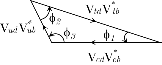
FIG. 1.: The unitarity triangle for B decays.

V Relation to the unitarity triangle

To conclude our discussion we explicitely restate the connections between the angles in the unitarity triangle, the CKM parameters and observable CP asymmetries.

The angles $\phi_{1}$, $\phi_{2}$ and $\phi_{3}$ are defined in Fig.1; as can be read off from Fig.2 they can be expressed by

$$\phi_{1} = \pi-\arg\left(\frac{-{\bf V}^{*}_{tb}{\bf V}_{td}}{-{\bf V}^{*}_{cb}{\bf V}_{cd}}\right),$$ (69)

$$\phi_{2} = \arg\left(\frac{{\bf V}^{*}_{tb}{\bf V}_{td}}{-{\bf V}^{*}_{ub}{\bf V}_{ud}}\right),$$ (70)

$$\phi_{3} = \arg\left(\frac{{\bf V}^{*}_{ub}{\bf V}_{ud}}{-{\bf V}^{*}_{cb}{\bf V}_{cd}}\right).$$ (71)

The CP asymmetry in $B_{d}\rightarrow\psi K_{S}$, which is driven by a single $\Delta B=1$ operator, is given by

$$A_{\psi K_{S}}={\rm sin}(\Delta M_{B}t)\mbox{Im}\,\left(\frac{q}{p}\overline{\rho}(\psi K_{S})\right)=$$

$$=\sin(2\phi_{1})\sin(|\Delta M_{B}|t)$$ (72)

To the degree we can eliminate the Penguin contribution to $B_{d}\rightarrow\pi^{+}\pi^{-}$ by, say, extracting the asymmetry for the isopin-two $\pi\pi$ final state, we have likewise:

$$A_{(\pi\pi)_{I=2}}={\rm sin}(\Delta M_{B}t)\mbox{Im}\,\left(\frac{q}{p}\overline{\rho}([\pi\pi]_{I=2})\right)=$$

$$=\mbox{Im}\,\left(\frac{V_{tb}V^{*}_{td}}{V^{*}_{tb}V_{td}}\frac{V_{ud}V^{*}_{ub}}{V^{*}_{ud}V_{ub}}\right){\rm sin}(|\Delta M_{B}t|)\simeq{\rm sin}(|\Delta M_{B}t|)\sin(2\phi_{2})$$ (73)

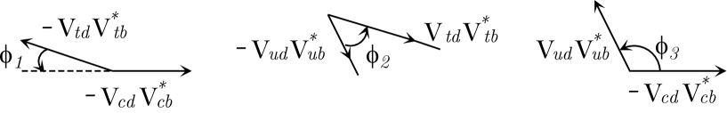
FIG. 2.: The unitarity triangle.

VI Summary

We have shown that the sign of the CP asymmetry in $B_{d}\rightarrow\psi K_{S}$ can be predicted within a given theory for $\Delta M_{B}$ and $\frac{q}{p}\bar{\rho}(\psi K_{S})$ even if the sign of $\Delta M_{B}$ cannot be determined experimentally. The same holds for $B_{d}\rightarrow\pi\pi$ etc. if one knows the weak operators driving these transitions.

En passant we have reminded the reader that the Standard Model can reproduce the observed sign of $\Delta M_{K}$ (and roughly its magnitude) through short-distance dynamics .

Our discussion illustrates that we can choose any convention we want – provided care is applied in treating everything consistently. We view it, however, as very useful to have a formalism for describing $B$ oscillations that parallels that for kaons. Furthermore it is much more natural to invoke theory to decide on the sign of $\Delta M_{B}$.

Acknowledgements

Work of IIB has been supported in part by the NSF under the grant number PHY 96-0508. Work of AIS has been supported in part by Grant-in-Aid for Special Project Research (Physics of CP violation).

REFERENCES

[1]
A. B. Carter and A. I. Sanda, Phys. Rev. D23 1567 (1981) .
[2]
I. I. Bigi and A. I. Sanda, Nucl. Phys. B193 85 (1981)
[3]K. Akerstaff, et al., Eur.Phys.J.C5 379,(1998).
[4] CDF Collaboration (T.J. LeCompte for the collaboration).
FERMILAB-CONF-98-293-E.
To be published in the proceedings of Workshop on CP Violation,
Adelaide, Australia, 3-8 Jul 1998.
[5]
Y. Grossman, B.Kayser and Y. Nir, Phys.Lett.B 415 90 (1997).
[6] Y. Nir and H. R. Quinn, in B decays Edited by S.
Stone World Scientific, Singapore, 1994.
[7]
I.I. Bigi and A.I. Sanda,
Phys. Lett. 148B (1984) 205-210.
[8]
M. Voloshin, M. Shifman, N. Uraltsev, and V. Khoze Sov. J. Nucl. Phys.46 112, (1987).
[9] I.I. Bigi, V. Khoze, A. Sanda and N. Uraltsev,
in: Edited by C. Jarlskog,
World Scientific, Singapore (1988).
[10]
G. Buchalla, A. J.Buras, and M. E. Lautenbacher,
Nucl. Phys. B370 69 (1992) ;
A. J. Buras, M. Jamin, and M. E. Lautenbacher,
Nucl. Phys. B408 209 (1993) .
[11]For a comprehensive review on hadronic matrix
elements see: A. Soni, Nucl. Phys. B47 (Proc. Suppl.)43 (1996) .