Cavendish-HEP-98/17

hep-ph/9811478

Effects of Perturbative Colour Interference on $WW\rightarrow\mbox{6-Jet}$ Distributions

Mark Smith
Cavendish Laboratory, University of Cambridge,

Madingley Road, Cambridge CB3 0HE, UK

26 November 1998

Abstract

At LEP II it is hoped to measure the W mass to an accuracy of around 40 MeV. This will require direct reconstruction of the mass of the W from its decay products in both the semi-leptonic and hadronic decay channels. Final state perturbative reconnection effects in hadronic decays are considered and their effect on 6-jet distributions and the reconstructed mass. The perturbative mass shift is found to be $\sim$ 50 keV in the negative direction.

1 Introduction

One of the main goals of LEP II will be an accurate determination of the mass of the W boson. An integrated luminosity of $500\mbox{ pb}^{-1}$ suggests that an accuracy of $30-50\mbox{ MeV}$ [1] could be reached. The process

$$e^{+}e^{-}\rightarrow W^{+}W^{-}\rightarrow\quad\mbox{4 fermions}$$ (1)

can be split into three distinct classes depending on the type of decay of each W-boson.

• Purely leptonic. Both W-bosons decay to leptons. There are two neutrinos and reconstruction of the event from observed charged lepton momenta is not possible. Branching ratio for this channel $\sim\frac{1}{9}$.

• Semi-leptonic. One W-boson decays to leptons, the other decays hadronically. One neutrino is produced, but the missing momentum can be reconstructed using energy-momentum conservation and assumptions about the initial state radiation. Branching ratio for this channel $\sim\frac{4}{9}$.

• Fully hadronic. Both W-bosons decay hadronically. All momenta are observable. The momenta directions are well resolved, while the energy resolution can be improved via kinematic fits (ie imposing the constraints of energy and momentum conservation). Branching ratio for this channel $\sim\frac{4}{9}$.

In order to achieve the greatest accuracy the W mass must be reconstructed using both the semi-leptonic and the fully hadronic decay channels. However W’s decay very rapidly so one expects that the space-time separation of the two decays should be $\sim 0.1\mbox{ fm}$. This is small compared to the typical scale of hadronization $\sim 1\mbox{ fm}$, thus in the case of fully hadronic decay there are two evolving hadronic systems with considerable space-time overlap. There is the possibility that the two systems do not evolve independently, but influence each other.

These influences fall into two categories - Bose-Einstein correlations between identical bosons in the final state (typically pions) [4, 5, 6], and a re-arrangement of the colour flow of the evolving systems at either the perturbative or hadronization level[7, 8, 9, 10]. There has been much work on the effects of colour re-arrangement at the hadronization level, however hadronization is poorly understood and progress can only be made through constructing models. It is interesting to note that the models of colour reconnections in the hadronization phase give rather varied predictions[1, 11] for the effects on physical observables such as mean charged multiplicity or reconstructed W mass, and so such measurements may probe directly aspects of the confinement mechanism.

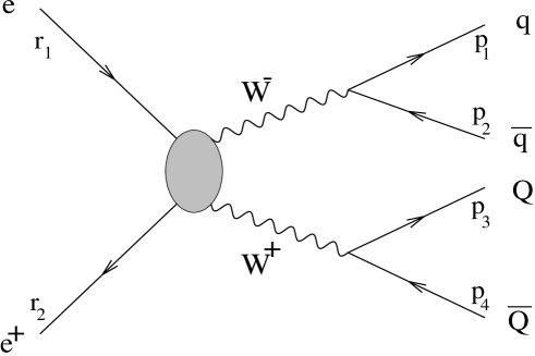
Figure 1: $e^{+}e^{-}\rightarrow W^{+}W^{-}\rightarrow q\bar{q}Q\bar{Q}$. The blob represents a sum over the three lowest order production amplitudes.

In this paper I will examine the effects of colour reconnection at its lowest non-trivial order in perturbation theory. In section two I will explain why these effects should be small and how they can be calculated directly. In section three I shall present results for the effects of colour reconnection on various distributions including the W mass. The conclusions will be found in section four.

2 Perturbative Reconnection

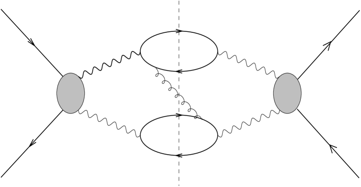
Figure 2: A possible interference term involving one exchanged gluon (the shaded blobs represent a sum over the three W-pair production amplitudes).

Perturbative reconnection appears as higher order corrections to the process shown in fig 1, in which gluons are exchanged between the evolving quark systems. A possible reconnection diagram is shown in fig 2; here a real gluon emitted from one decay system interferes with the similar emission from the other decay system. One may also consider the analogous virtual interference corresponding to the exchange of a virtual gluon between decay systems. Within perturbation theory these interference terms are zero due to colour conservation, and so one must consider the exchange of at least two perturbative gluons.

A full calculation of the $\mathcal{O}(\alpha_{s}^{2})$ corrections is beyond the scope of this paper, however it is possible to examine QCD interference effects in the production of 6 jets[12] via

$$e^{+}e^{-}\rightarrow W^{+}W^{-}\rightarrow q\bar{q}q\bar{q}gg$$ (2)

in which interferences appear between the lowest order diagrams. Two possible interference terms are shown in fig 3.

Figure 3: Interference terms involving the exchange of two gluons (the W-pair production parts of the diagrams are omitted for clarity)

These diagrams contain only two colour loops, compared with the diagrams for gluon emissions within each decay system which contain four loops. Therefore the interference terms are suppressed relative to the leading emission by $\frac{1}{N_{C}^{2}}$ where $N_{C}$ is the number of colours.

There is further suppression due to the width of the W. Gluons radiated within a decay system are free to have any energy up to $\sim M_{W}$ without pushing the W Breit-Wigner propagators off resonance. However gluons radiated between the decay systems (interference terms) must carry energy less than $\sim\Gamma_{W}$ or at least two of the W propagators must be pushed off resonance and that term will become suppressed. It has been shown that for inclusive quantities, where the I.R divergences cancel between real and virtual diagrams, that this leads to a suppression of perturbative reconnection effects by $\mathcal{O}(\frac{\Gamma_{W}}{M_{W}})$[13, 15]. A rough estimate of the size of perturbative reconnection effects in W-pair production is thus:

$$\frac{\Delta\sigma}{\sigma_{0}}\sim\frac{\alpha_{s}^{2}}{N_{C}^{2}}\frac{\Gamma_{W}}{M_{W}}\sim 10^{-4}$$ (3)

and so one may estimate the possible mass shift as

$$\Delta M_{W}\sim\frac{\alpha_{s}^{2}}{N_{C}^{2}}\Gamma_{W}\sim\mbox{a few MeV}$$ (4)

This should be regarded as an order of magnitude estimate only. It is clearly desirable to calculate experimental distributions in fixed order perturbation theory and examine how they may be distorted by the effects of colour interference.

Using the helicity methods of [15] it is possible to construct the amplitudes for all the doubly resonant diagrams contributing to the $q\bar{q}q\bar{q}gg$ final state; there are 72 diagrams in total. In this method each amplitude is built up from relatively few component pieces that can be calculated separately. For example the amplitude for fig 1 can be written

Figure 4: Components used to calculate lowest order $e^{+}e^{-}\rightarrow W^{+}W^{-}\rightarrow q\bar{q}q\bar{q}$. The shaded blob represents the sum of the three interfering amplitudes, and the WW propagators have been absorbed into the definition of $T^{\mu\nu}$

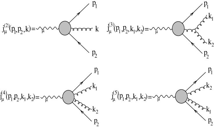
Figure 5: Additional components needed to calculate the doubly resonant contributions to $e^{+}e^{-}\rightarrow q\bar{q}q\bar{q}gg$. The shaded blob represents a sum over possible attachments of gluons to the spinor line which preserve the order of attachments.

$$\mathcal{M}(r_{1},r_{2};p_{1},p_{2},p_{3},p_{4})=T^{\mu\nu}(r_{1},r_{2};p_{1}+p_{2},p_{3}+p_{4})j^{(1)}_{\mu}(p_{1},p_{2})j^{(1)}_{\nu}(p_{3},p_{4})$$ (5)

where the terms are defined in fig 4 and the momentum labels refer to fig 1. The computational complexity is reduced by assuming massless electrons and massless quarks which has been done throughout this paper.

In this way all of the amplitudes can be built up from just the production tensor $T^{\mu\nu}$ and some ‘decay currents’ $j^{(i)}_{\mu}$. In order to calculate all amplitudes for double gluon radiation four additional decay currents (fig 5) are needed. Note one must distinguish between $j^{(4)}_{\mu}$ and $j^{(5)}_{\mu}$ which are related by $j^{(4)}_{\mu}=j^{(5)}_{\mu}(k_{1}\leftrightarrow k_{2})$ in order to obtain the correct colour factors.

The decay currents may be contracted onto the production tensor to obtain eight distinct Lorentz-colour structures (colour-matrices are omitted for clarity)

$$\mathcal{M}_{1} = T^{\mu\nu}j^{(2)}_{\mu}(p_{1},p_{2},k_{1})j^{(2)}_{\nu}(p_{3},p_{4},k_{2})$$

$$\mathcal{M}_{2} = \mathcal{M}_{1}(k_{1}\leftrightarrow k_{2})$$

$$\mathcal{M}_{3a} = T^{\mu\nu}j^{(4)}_{\mu}(p_{1},p_{2},k_{1},k_{2})j^{(1)}_{\nu}(p_{3},p_{4})$$

$$\mathcal{M}_{3b} = T^{\mu\nu}j^{(5)}_{\mu}(p_{1},p_{2},k_{1},k_{2})j^{(1)}_{\nu}(p_{3},p_{4})$$

$$\mathcal{M}_{4a} = T^{\mu\nu}j^{(1)}_{\mu}(p_{1},p_{2})j^{(4)}_{\nu}(p_{3},p_{4},k_{1},k_{2})$$

$$\mathcal{M}_{4b} = T^{\mu\nu}j^{(1)}_{\mu}(p_{1},p_{2})j^{(5)}_{\nu}(p_{3},p_{4},k_{1},k_{2})$$

$$\mathcal{M}_{5} = T^{\mu\nu}j^{(3)}_{\mu}(p_{1},p_{2},k_{1},k_{2})j^{(1)}_{\nu}(p_{3},p_{4})$$

$$\mathcal{M}_{6} = T^{\mu\nu}j^{(1)}_{\mu}(p_{1},p_{2})j^{(3)}_{\nu}(p_{3},p_{4},k_{1},k_{2})$$ (6)

then the total production amplitude is (suppressing colour matrices)

$$\mathcal{M}=\mathcal{M}_{1}+\mathcal{M}_{2}+\mathcal{M}_{3a}+\mathcal{M}_{3b}+\mathcal{M}_{4a}+\mathcal{M}_{4b}+\mathcal{M}_{5}+\mathcal{M}_{6}$$ (7)

after squaring and summing over colours it is convenient to separate the squared matrix element into different parts depending on the form of the Breit-Wigner resonances. In this way one finds six distinct terms

$$\sum_{colours}|\mathcal{M}|^{2}=M_{1}+M_{2}+M_{3}+M_{4}+M_{5}+M_{6}$$ (8)

where

$$M_{1} = N_{C}^{2}C_{F}^{2}\mathcal{M}_{1}\mathcal{M}_{1}^{*}$$ (9)

$$M_{2} = M_{1}(k_{1}\leftrightarrow k_{2})$$ (10)

$$M_{3} = N_{C}^{2}C_{F}^{2}(\mathcal{M}_{3a}\mathcal{M}_{3a}^{*}+\mathcal{M}_{3b}\mathcal{M}_{3b}^{*})+N_{C}^{3}C_{F}\mathcal{M}_{5}\mathcal{M}_{5}^{*}-$$ (11)

$$\frac{1}{2}N_{C}C_{F}(\mathcal{M}_{3a}\mathcal{M}_{3b}^{*}+\mathcal{M}_{3b}\mathcal{M}_{3a}^{*})+$$

$$\frac{1}{2}N_{C}^{3}C_{F}([\mathcal{M}_{3a}\mathcal{M}_{5}^{*}+\mathcal{M}_{5}\mathcal{M}_{3a}^{*}]-[\mathcal{M}_{3b}\mathcal{M}_{5}^{*}+\mathcal{M}_{5}\mathcal{M}_{3b}^{*}])$$

$$M_{4} = N_{C}^{2}C_{F}^{2}(\mathcal{M}_{4a}\mathcal{M}_{4a}^{*}+\mathcal{M}_{4b}\mathcal{M}_{4b}^{*})+N_{C}^{3}C_{F}\mathcal{M}_{5}\mathcal{M}_{5}^{*}-$$ (12)

$$\frac{1}{2}N_{C}C_{F}(\mathcal{M}_{4a}\mathcal{M}_{4b}^{*}+\mathcal{M}_{4b}\mathcal{M}_{4a}^{*})+$$

$$\frac{1}{2}N_{C}^{3}C_{F}([\mathcal{M}_{4a}\mathcal{M}_{5}^{*}+\mathcal{M}_{5}\mathcal{M}_{4a}^{*}]-[\mathcal{M}_{4b}\mathcal{M}_{5}^{*}+\mathcal{M}_{5}\mathcal{M}_{4b}^{*}])$$

$$M_{5} = \frac{1}{2}N_{C}C_{F}(\mathcal{M}_{1}\mathcal{M}_{2}^{*}+\mathcal{M}_{2}\mathcal{M}_{1}^{*})$$ (13)

$$M_{6} = \frac{1}{2}N_{C}C_{F}[(\mathcal{M}_{3a}+\mathcal{M}_{3b})(\mathcal{M}_{4a}+\mathcal{M}_{4b})^{*}+$$ (14)

$$(\mathcal{M}_{4a}+\mathcal{M}_{4b})(\mathcal{M}_{3a}+\mathcal{M}_{3b})^{*}]$$

In the above expression the terms $M_{1},M_{2},M_{3},M_{4}$ denote the unreconnected parts, while $M_{5}$ and $M_{6}$ correspond to interference between the two decays. The separation into reconnected and unreconnected parts is (QCD) gauge invariant.

One can find small regions of phase space where the interference contribution to the total transition probability is as large as 10%, even for relatively energetic gluons ($\geq 5\mbox{ GeV}$). It is therefore not impossible that certain 6 jet distributions could be significantly distorted by perturbative reconnection.

A Monte Carlo program was written to generate WW events with the $q\bar{q}q\bar{q}gg$ final state using the Multichannel approach [16] with 24 channels based on the kinematic properties of the contributing diagrams. Events were generated at a centre-of-mass energy of $192\mbox{ GeV}$, although reconnection effects are expected to be insensitive to the centre-of-mass energy within the LEP II range. In addition specific phase space parameterisations were computed which allowed efficient integration of both types of interference term.

Six jet final states were defined according to a minimum invariant mass between partons. A lower limit of $s_{cut}=1\mbox{ GeV}^{2}$ was used. Strictly speaking this is too small for fixed order perturbation theory to be applicable, however the philosophy is that the results obtained will provide an upper limit on reconnection effects, since moving to larger values of $s_{cut}$ generally reduces any effect. The six partons were clustered to four jets using the Durham algorithm[17]. Distributions for the Bengtsson-Zerwas angle[18] $(\chi_{BZ})$, the modified Nachtmann-Reiter angle[19] $(\theta_{NR})$ and the angle between the two lowest energy jets $(\alpha_{34})$ were computed with and without the interference terms. These angles are defined by equation 15 below in which $\mathbf{p_{1},p_{2},p_{3}}$ and $\mathbf{p_{4}}$ are the energy ordered jet 3-momenta.

$$\cos(\chi_{BZ}) = \mathbf{\frac{(p_{1}\times p_{2})\cdot(p_{3}\times p_{4})}{|p_{1}\times p_{2}||p_{3}\times p_{4}|}}$$

$$\cos(\theta_{NR}) = \mathbf{\frac{(p_{1}-p_{2})\cdot(p_{3}-p_{4})}{|p_{1}-p_{2}||p_{3}-p_{4}|}}$$ (15)

With four jets there are three ways of pairing them. For each pairing the average of the invariant masses was computed. Thus for each event one has three mass values corresponding to each of the three possible pairings. The mass closest to the input W mass was chosen as the mass estimate (this is only one of several possibilities suggested in [5]). Distributions for the mass calculated in this way were also produced with and without colour interference terms.

The difference between distributions with and without the interference terms was computed. This shows the distortion induced by the interferences.

Finally the integral of the absolute value of the interferences was found for gluon energies greater than $2\mbox{ GeV}$, $5\mbox{ GeV}$ and $10\mbox{ GeV}$. These quantities are finite since the interference terms contain no collinear singularities (apart from integrable ones when three partons become collinear), and provide an indication of the possible size of interference effects in events with jet energies greater than $2,5$ and $10\mbox{ GeV}$.

3 Results

The mean mass can be calculated with and without the reconnected terms. The result one finds depends on the choice of invariant mass cut, but must tend to zero as $s_{cut}\rightarrow 0$ since the unreconnected terms are more singular than the reconnected terms in this limit. Mass shifts for a variety of invariant mass cuts on the final state are shown in the table below.

$s_{cut}/\mbox{GeV}^{2}$	$0.1$	$1.0$	$10.0$	$100.0$
$\delta M_{W}/\mbox{MeV}$	$-0.030$	$-0.045$	$-0.025$	$\sim-0.015$

The exact numbers are also slightly dependent on the reconstruction scheme used for defining the experimental W mass.

Figure 6: Mass distribution for unreconnected events (solid line), change induced by reconnected terms $\times 1000$ (dashed line), in arbitrary units

Figure 7: Distribution of $\chi_{BZ}$, the Bengtsson-Zerwas Angle for unreconnected events (solid line), change induced by reconnected terms $\times 1000$ (dashed line)

Figure 8: Distribution of $\cos(\alpha_{34})$ for unreconnected events (solid line), change induced by reconnected terms $\times 500$ (dashed line), in arbitrary units

Figure 9: Distribution of $\cos(\theta_{NR})$, the Nachtmann-Reiter Angle for unreconnected events (solid line), change induced by reconnected terms $\times 500$ (dashed line)

Figure 6 shows the distribution of reconstructed mass using only the unreconnected parts of the matrix element (solid line). The dashed line shows one thousand times the change induced when the reconnected terms are present. The distributions for the mass under the full matrix element and unreconnected terms only differ essentially by a multiplicative constant of order $1.001$. The mean value of the mass distribution is shifted by less than a part per million due to the presence of reconnected terms.

Figures 7,8 and 9 show similar plots for the distribution of the Bengtsson-Zerwas angle, the angle between the two lowest energy jets $\alpha_{34}$ and the Nachtmann-Reiter angle. It will be seen that the effect is at or below the per mille level and is essentially just multiplicative, distortions of the distributions occur at a much lower level. These effects can be understood within the soft interference limit. In the soft limit one may describe gluon radiation using eikonal vertices and the matrix element squared becomes.

$$|\mathcal{M}|^{2}=|\mathcal{M}_{0}|^{2}(H(k_{1},k_{2})+AG(k_{1})G(k_{2}))$$ (16)

where $H(k_{1},k_{2})$ is the soft unreconnected distribution, A is some constant that will depend on the energy resolution and W width. $G(k)$ is the reconnected distribution (note that at this order the reconnected gluons are radiated independently, however this is not true in higher orders) and is given by

$$G(k)=\frac{(p_{1}\cdot p_{4})}{(p_{1}\cdot k)(p_{4}\cdot k)}+\frac{(p_{2}\cdot p_{3})}{(p_{2}\cdot k)(p_{3}\cdot k)}-\frac{(p_{1}\cdot p_{3})}{(p_{1}\cdot k)(p_{3}\cdot k)}-\frac{(p_{2}\cdot p_{4})}{(p_{2}\cdot k)(p_{4}\cdot k)}$$ (17)

One may integrate over the directions of each emission to find the enhancement due to soft interference between decays:

$$|\mathcal{M}_{rec}|^{2}\sim|\mathcal{M}_{0}|^{2}\times\ln^{2}\left(\frac{(p_{1}\cdot p_{4})(p_{2}\cdot p_{3})}{(p_{1}\cdot p_{3})(p_{2}\cdot p_{4})}\right)$$ (18)

where the momenta are as defined in fig 1.

The effect of the reconnection terms is essentially to enhance coplanar configurations where some invariant masses can be much larger than others. In configurations where the W decay planes are at right angles, none of the parton directions can become close and so the argument of the logarithm in equation (18) is close to one and there is little enhancement. In most approximately coplanar configurations the BZ angle will be close to either $0$ or $\pi$ as both $\mathbf{p_{1}\times p_{2}}$ and $\mathbf{p_{3}\times p_{4}}$ (energy ordered momenta) are likely to point out of the decay plane and hence be either parallel or anti-parallel. Thus one expects enhancement around these values.

The situation for $\cos(\alpha_{34})$ is not quite so straight forward. A similar argument favours $\cos(\alpha_{34})\sim 1$ however this configuration is suppressed by the jet reconstruction kinematics; one would need two low energy quarks and both gluons radiated in approximately the same direction and to be clustered as two distinct jets. However the configurations corresponding to $\cos(\alpha_{34})\sim-1$ can be enhanced (see fig 10).

A similar argument for $\theta_{NR}$ is not so apparent as its geometrical interpretation is less clear (the angle between the axis defined by the vector between the two lowest energy jets and that between the two highest energy jets). One may construct the enhancement due to equation (18) and find qualitatively the same shape as observed in figure 9.

Figure 10: Kinematic configurations which are a) Enhanced by interference but kinematically suppressed ($\cos(\alpha_{34})\sim 1$), and b) Enhanced by interference ($\cos(\alpha_{34})\sim-1$), since $(p_{1}\cdot p_{4})(p_{2}\cdot p_{3})>(p_{1}\cdot p_{3})(p_{2}\cdot p_{4})$. The momentum labels refer to fig 1, and in this example $p_{2}$ and $p_{3}$ correspond to the lowest energy jets.

The absolute value of the interference terms was integrated over the region defined by $\omega\geq 2\mbox{ GeV}$, $\omega\geq 5\mbox{ GeV}$ and $\omega\geq 10\mbox{ GeV}$ where $\omega$ is the minimum gluon energy. This was done for $s_{cut}=10,1.0,0.1,0.01\mbox{ GeV}^{2}$ and illustrates collinear finiteness (see results below).

$\sigma_{|int|}/\mbox{pb}$		$s_{cut}/\mbox{GeV}^{2}$
		$10$	$1.0$	$0.1$	$0.01$
	2	0.015	0.029	0.032	0.033
$\omega/\mbox{GeV}$	5	$0.0057$	$0.0082$	$0.009$	$0.01$
	10	$0.0016$	$0.0023$	$0.0026$	$0.0026$

The errors on these numbers are around 4% each. Note that these are the integrated absolute value of the interference terms, the actual contribution of the interference terms to the cross-section is typically an order of magnitude smaller due to large cancellations.

4 Conclusions

Effects of perturbative reconnection are not necessarily small, however the regions of phase space in which sizable effects can occur are small. Most experimentally interesting distributions are unaffected by reconnection at the perturbative level apart from a multiplicative factor close to unity. In particular the mass distribution is shifted by less than one part per million by lowest order reconnection effects in 6-jet events. Distributions sensitive to soft momenta seem to show greater distortion, however these effects are well below the per mille level and so unlikely to be seen at LEP II.

The integration of the absolute value of the reconnection terms for gluon energies above $5\mbox{ GeV}$ shows that the maximum effect could only be equivalent to a few events at LEP II and can probably be neglected at this level of statistics.

Of course reconnection effects summed over higher terms, or within the hadronization phase need not be negligible and these effects still need to be addressed.

References

- [1] Z. Kunszt, W.J. Stirling et al., CERN-96-01 (1996) Vol1 p141
- [2] W. Beenakker, A. P. Capovsky and F. Berends, Phys. Lett. B411 (1997) 203
- [3] A. Denner, S. Dittmaier and M. Roth, Nucl. Phys. B519 (1998) 39
- [4] L. Lonnblad and T. Sjostrand, Phys. Lett. B351 (1995) 293
- [5] J. Hakkinen and M. Ringner, Eur. Phys. J. C5 (1998) 275
- [6] V. Kartvelishvili, R. Kvatadze and R. Moller, Phys. Lett. B408 (1997) 331
- [7] T. Sjostrand and V. A. Khoze, Z. Phys. C62 (1994) 281
- [8] T. Sjostrand and V. A. Khoze, Phys. Rev. Lett. 72 (1994) 28
- [9] C. Friberg and G. Gustafson and J. Hakkinen, Nucl.Phys. B490 (1997) 289
- [10] J. Ellis and K. Geiger, Phys. Rev. D 54 (1996) 1967
- [11] P. B. Renton, W. J. Stirling, D. R. Ward et al., J. Phys. G:Nucl. Part. Phys. 24 (1998) 365
- [12] E. Accomando, A. Ballestrero and E. Maina, Phys. Lett. B362 (1995) 141
- [13] V. S. Fadin, V. A. Khoze and A. D. Martin, Phys. Rev. D 49 (1994) 2247
- [14] V. S. Fadin, V. A. Khoze and A. D. Martin, Phys. Lett. B320 (1994) 141
- [15] A. Ballestrero and E. Maina, Phys. Lett. B350 (1995) 225
- [16] R. Kleiss and R. Pittau, Comput. Phys. Commun. 83 (1994) 141
- [17] S. Catani, Y. L. Dokshitser, M. Olsson, G. Turnock and B. R. Webber, Phys. Lett. B269 (1991) 432
- [18] M. Bengtsson and P. M. Zerwas, Phys. Lett. B208 (1998) 306
- [19] S. Bethke, A. Richter and P. M. Zerwas, Z. Phys. C49 (1991) 59