The $\Delta I=1/2$ Rule in the Chiral Limit

Abstract:

We discuss the matching between long-distance and short-distance at next-to-leading in $1/N_{c}$ and show how the scheme-dependence from the two-loop renormalization group running can be treated. We then use this method to study the three $O(p^{2})$ terms contributing to non-leptonic kaon decays, namely the usual octet and 27-plet derivative terms as well as the weak mass term using the Extended Nambu–Jona-Lasinio model as the low energy approximation. We also discuss subtleties in the momentum routing in the low energy theory and a problem in separating factorizable and non-factorizable contributions from the $Q_{6}$ operator in the chiral limit. We update our earlier results on the $B_{K}$ parameter as well.

1 Introduction

The $\Delta I=1/2$ rule in kaon decays has been the subject of very many efforts at understanding it, see [1] for a review. We briefly discuss it and a short history of attempts to understand it in Section 2. In this paper we attempt to put together various approaches that have been done before. The short-distance effects are now known to two-loops and the extended Nambu–Jona-Lasinio Model enhanced by using Chiral Perturbation Theory whenever possible provides a reasonable basis for the long-distance description of hadronic interactions needed. We put the two together in a way that treats the scheme dependence correctly. The underlying method, reproducing the results of the short-distance running by an effective theory of exchanges of heavy bosons, which we call $X$-bosons, is discussed in Section 3.2. The low energy model is shortly discussed in Section 3.3. In Section 3.1 we recall the definitions of the off-shell two-point functions that we use here to determine the weak non-leptonic couplings. The method here is basically to calculate these two-point functions to next-to-leading order in $1/N_{c}$, but to all orders in the terms enhanced by large logarithms involving $M_{W}$. We then compare with the Chiral Perturbation Theory (CHPT) calculations of the same quantity and in the end we calculate the relevant physical matrix elements using CHPT.

In Section 4 we update our earlier results for $B_{K}$[2]. Here we discuss in some detail the routing issue in Section 4.1, which is rather non-trivial in the presence of neutral $X$-bosons whose direction is not obvious. This also explains the discrepancies of the results for very low $\mu$ in the chiral limit of [2] and the results of [3]. We give therefore updated numbers and expressions for the main results of [2] here.

Section 5 contains the same discussion but for the $\Delta S=1$ operators $Q_{1}$ to $Q_{6}$. The current$\times$current operators $Q_{1}$, $Q_{2}$, and $Q_{3}$ are computed at next-to-leading (NLO) in $1/N_{c}$ within the ENJL model. The split in Penguin-like and $B_{K}$-like contributions is discussed. For $Q_{5}$ we cannot simply discuss this split, here the correct chiral behaviour is only reproduced after summing both contributions.

When extending the method to $Q_{6}$ one discovers that the factorizable contribution from $Q_{6}$ has an infrared divergence in the chiral limit. We discuss this problem in Section 5.2 and show how it is cancelled by the non-factorizable contribution. This problem might be part of the reason why estimates for the $Q_{6}$ operator vary so widely. After correcting for this we present also results for the matrix elements of $Q_{6}$.

Finally we put the numerical results for the long- and short-distances together in Section 6 and discuss their stability. We also discuss here the coefficients $a$, $b$, and $c$ defined earlier by Pich and de Rafael [4]. We recapitulate our main results and conclusions in Section 7

2 The $\Delta I=1/2$ Rule in $K\to\pi\pi$

The $K\to\pi\pi$ invariant amplitudes can be decomposed into definite isospin quantum numbers amplitudes as $[A\equiv-iT]$

$$A[K_{S}\to\pi^{0}\pi^{0}] \equiv \sqrt{2\over 3}A_{0}-{2\over\sqrt{3}}A_{2}\,;$$

$$A[K_{S}\to\pi^{+}\pi^{-}] \equiv \sqrt{2\over 3}A_{0}+{1\over\sqrt{3}}A_{2}\,;$$

$$A[K^{+}\to\pi^{+}\pi^{0}] \equiv {\sqrt{3}\over 2}A_{2}\,.$$ (1)

Where $K_{S}\simeq K_{1}^{0}+\epsilon\,K_{2}^{0}$, $K^{0}_{1(2)}\equiv(K^{0}-(+)\overline{K^{0}})/\sqrt{2}$, and CP($K^{0}_{1(2)})=+(-)K^{0}_{1(2)}$. In this paper we are interested in the CP conserving part of $K\to\pi\pi$, so we set the small phase in the Standard Model CKM matrix elements and therefore $\epsilon$ to zero. Above we have included the final state interaction phases $\delta_{0}$ and $\delta_{2}$ into the amplitudes $A_{0}$ and $A_{2}$ as follows. For the isospin $1/2$ amplitude

$$A_{0}\equiv-ia_{0}\,e^{i\delta_{0}}\,,$$ (2)

and for the isospin $3/2$

$$A_{2}\equiv-ia_{2}\,e^{i\delta_{2}}\,.$$ (3)

With the measured $K_{S}\to\pi^{0}\pi^{0}$ partial width $\Gamma_{00}$, $K_{S}\to\pi^{+}\pi^{-}$ partial width $\Gamma_{+-}$, and $K^{+}\to\pi^{+}\pi^{0}$ partial width $\Gamma_{+0}$ [5], we can calculate the ratio

$$\left|\frac{A_{0}}{A_{2}}\right|=\left({3\over 4}\sqrt{\frac{1-4m_{\pi}^{2}/m_{K^{+}}^{2}}{1-4m_{\pi}^{2}/m_{K^{0}}^{2}}}\left(\frac{\Gamma_{00}+\Gamma_{+-}}{\Gamma_{+0}}\right)-1\right)^{1/2}=22.10$$ (4)

This result is what is called the $\Delta I=1/2$ rule for kaon decays.

To understand quantitatively this rule has been one of the permanent issues in the literature since the experimental determination. It is by now clear that it is the sum of several large contributions both from short distance origin [6, 7] and from long distance origin [8, 9, 10] which add constructively to make $|A_{0}|$ much larger than $|A_{2}|$.

The lattice QCD community has also spent a large effort on this problem, see [11] for some recent reviews.

Among the long distance enhancements of the $|A_{0}/A_{2}|$ ratio, the order $p^{4}$ chiral corrections have been found to be quite important. The CHPT analysis to order $p^{4}$ can be found in [10] and both the counter-terms and the chiral logs to that order can be found in [12], the chiral logs were originally calculated in [13]. There are some small differences between the two results. The fit of the data to both the order $p^{4}$ $K\to\pi\pi$ and $K\to\pi\pi\pi$ counter-terms and chiral logs [10, 14] allowed to extract

$$\left|\frac{A_{0}}{A_{2}}\right|^{(2)} = 16.4$$ (5)

to $O(p^{2})$, i.e., around 34 % of the enhancement in the $\Delta I=1/2$ rule is due just to order $p^{4}$ and higher CHPT corrections.

2.1 CHPT to order $p^{2}$

To order $p^{2}$ in CHPT, the amplitudes $a_{0}$ and $a_{2}$ can be written in terms of two couplings,

$$a_{0}\equiv a_{0}^{8}+a_{0}^{27} = C\,\left[9G_{8}+G_{27}\right]\frac{\sqrt{6}}{9}F_{0}(m_{K}^{2}-m_{\pi}^{2})\,,$$

$$a_{2} = C\,G_{27}\frac{10\sqrt{3}}{9}F_{0}(m_{K}^{2}-m_{\pi}^{2})\,,$$ (6)

with

$$C\equiv-\frac{3}{5}\,\frac{G_{F}}{\sqrt{2}}\,V_{ud}\,V_{us}^{*}\approx-1.06\cdot 10^{-6}\,\mbox{GeV}^{-2}$$ (7)

and

$$\delta_{0}=\delta_{2}=0\,.$$ (8)

The couplings $G_{8}$ and $G_{27}$ are two of the $O(p^{2})$ $\Delta S=1$ couplings. They are defined in [12] and can be determined from the $O(p^{2})$ amplitudes [14] to be

$$G_{8}=6.2\pm 0.7\qquad{\rm and}\qquad G_{27}=0.48\pm 0.06\,.$$ (9)

Here we have only included the error bars from the value of the pion decay constant in the chiral limit $F_{0}=(86\pm 10)$ MeV, this corresponds to $f_{\pi}=92.4$ MeV. Again there are uncertainties from the fit procedure and approximations not quoted in [10, 14].

Therefore to $O(p^{2})$

$$\left|\frac{A_{0}}{A_{2}}\right|^{(2)}=\sqrt{2}\,\left(\frac{9\,G_{8}+G_{27}}{10\,G_{27}}\right)\,.$$ (10)

To understand the difficulty of the task of reproducing (5) it is convenient to make an $1/N_{c}$ analysis of the $O(p^{2})$ result. At large $N_{c}$, $G_{8}=G_{27}=1$ and

$$\left|\frac{A_{0}}{A_{2}}\right|^{(2)}_{N_{c}}=\sqrt{2}$$ (11)

i.e. a factor 11.6 smaller than the QCD result in (5) ! Notice that to $O(p^{2})$ there are no quark mass and therefore no chiral logs corrections to the ratio above. So we have to explain one order of magnitude enhancement within QCD in the chiral limit with $1/N_{c}$ suppressed corrections.

Another parametrization which will be useful when studying the $\Delta I=1/2$ rule is the one introduced by Pich and de Rafael in [4]. In this parametrization

$$G_{27} \equiv a+b\,,$$

$$G_{8} \equiv a+b+{5\over 3}(c-b)\,.$$ (12)

The nice feature of this parametrization is that $a$, $b$, and $c$ have a one to one correspondence with the three-different QCD quark-level topologies. The $a$-type coupling corresponds to configurations that include the factorizable ones (Figure 1a). This coupling is of order 1 in the large $N_{c}$ limit and has only $1/N_{c}^{2}$ corrections. The $b$-type coupling corresponds to what we call $B_{K}$-like topologies (Figure 1b) and is of order $1/N_{c}$. This coupling is related to the value of the $B_{K}$ parameter in the chiral limit.

The $c$-type coupling corresponds to what we call Penguin-like topologies (Figure 1c) and is also of order $1/N_{c}$. So in the large $N_{c}$ limit

$$a=1\hskip 28.45274pt{\rm and}\hskip 28.45274pt\;b=c=0\;.$$ (13)

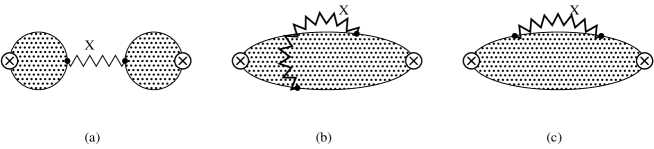
Figure 1: The three types of contributions appearing in the evaluation of matrix-elements of operators. Namely, (a) Factorizable, (b) $B_{K}$-like, and (c) Penguin-like.

The main objective of this paper is the calculation of the $1/N_{c}$ corrections to (11), i.e. the couplings $b$ and $c$.

The coefficients $a$, $b$, and $c$ in [4] were defined in a large $N_{c}$ expansion within short-distance QCD, i.e. with quarks and gluons. In the low-energy regime where the long-distance part has to be evaluated one however cannot distinguish the $1/N_{c}^{2}$ corrections to $a$ from the ones to the coefficients $b$ and $c$. So for us $a$ takes the large $N_{c}$ value $a=1$, $b=G_{27}-1$, and $c=(3G_{8}+2G_{27})/5-1$. This definition can be used both at long and short-distances and only differs by terms of $O(1/N_{c}^{2})$ with the one in [4]. The definition above has also the advantage that all couplings $a$, $b$, and $c$ are scale independent. Notice that in the present work the $1/N_{c}^{2}$ are from short-distance origin only.

3 The Technique

3.1 $\Delta S=1$ and $\Delta S=2$ Two-Point Functions

The theoretical framework we use to study the strangeness changing transitions in one and two units was already introduced in Refs. [2, 12, 15]. The original suggestion for this type of method was in [16]. The basic objects are the pseudo-scalar density correlators

$$\Pi^{ij}(q^{2})\equiv i\int{\rm d}^{4}x\,e^{iq.x}\langle 0|T\left(P^{i\dagger}(0)P^{j}(x)e^{i\Gamma_{\Delta S=a}}\right)|0\rangle$$ (14)

in the presence of strong interactions. Above, $a=0,1,2$ stands for $|\Delta S|=$ 0, 1, and 2 transitions and $i,j$ are light quark combinations corresponding to the octet of the lightest pseudo-scalar mesons;

$$P^{\pi^{0}}(x)\equiv\frac{\displaystyle 1}{\displaystyle\sqrt{2}}\left[\overline{u}i\gamma_{5}u-\overline{d}i\gamma_{5}d\right]\,, P^{\pi^{+}}(x)\equiv\left[\overline{d}i\gamma_{5}u\right]\,,P^{K^{0}}(x)\equiv\left[\overline{s}i\gamma_{5}d\right]\,,$$

$$P^{K^{+}}(x)\equiv\left[\overline{s}i\gamma_{5}u\right]\,, P^{\eta_{8}}(x)\equiv\frac{\displaystyle 1}{\displaystyle\sqrt{6}}\left[\overline{u}i\gamma_{5}u+\overline{d}i\gamma_{5}d-2\overline{s}i\gamma_{5}s\right]\,.$$

Here and in the remainder, summation over colour-indices inside brackets is assumed unless colour indices have been explicitly indicated. These two-point functions were analyzed extensively within CHPT to order $p^{4}$ in [12]. In that reference we also pointed out how on can obtain information on $K\to\pi\pi$ amplitudes at order $p^{4}$ from off-shell $K\to\pi$ transitions.

Now, we want to use the $1/N_{c}$ technique used in [2, 15] to compute the off-shell $K\to\pi$ amplitudes and obtain the relevant counter-terms of order $p^{2}$. See [12], for explicit details of which counter-terms of order $p^{4}$ we can get and possible ways of estimating some couplings we cannot get this way.

In the large $N_{c}$ limit, there is just one operator in the Standard Model which changes strangeness by one-unit

$$Q_{2}\equiv[\bar{s}\gamma^{\mu}(1-\gamma_{5})u](x)[\bar{u}\gamma_{\mu}(1-\gamma_{5})d](x)\,.$$ (16)

After the inclusion of gluonic corrections $Q_{2}$ mixes with

$$Q_{1}\equiv[\bar{s}\gamma^{\mu}(1-\gamma_{5})d](x)[\bar{u}\gamma_{\mu}(1-\gamma_{5})u](x)$$ (17)

via box-type diagrams (first reference in [6]), and with

$$Q_{3} \equiv [\bar{s}\gamma^{\mu}(1-\gamma_{5})d](x)\sum_{q=u,d,s}[\bar{q}\gamma_{\mu}(1-\gamma_{5})q](x)$$

$$Q_{4} \equiv [\bar{s}^{\alpha}\gamma^{\mu}(1-\gamma_{5})d_{\beta}](x)\sum_{q=u,d,s}[\bar{q}^{\beta}\gamma_{\mu}(1-\gamma_{5})q_{\alpha}](x)$$

$$Q_{5} \equiv [\bar{s}\gamma^{\mu}(1-\gamma_{5})d](x)\sum_{q=u,d,s}[\bar{q}\gamma_{\mu}(1+\gamma_{5})q](x)$$

$$Q_{6} \equiv [\bar{s}^{\alpha}\gamma^{\mu}(1-\gamma_{5})d_{\beta}](x)\sum_{q=u,d,s}[\bar{q}^{\beta}\gamma_{\mu}(1+\gamma_{5})q_{\alpha}](x)$$ (18)

via the so-called penguin-type diagrams [6]. Since the numerical importance for the issues we want to address here is small and for the sake of simplicity we switch off electromagnetic interactions. The operator $Q_{4}$ is redundant and satisfies $Q_{4}=Q_{2}-Q_{1}+Q_{3}$. Under SU(3)_L$\times$SU(3)_R rotations $Q_{-}\equiv Q_{2}-Q_{1}$, $Q_{3}$, $Q_{4}$, $Q_{5}$, and $Q_{6}$ transform as $8_{L}\times 1_{R}$ and only carry $\Delta I=1/2$ while $Q_{27}\equiv 3Q_{1}+2Q_{2}-Q_{3}$ transforms as $27_{L}\times 1_{R}$ and carries both $\Delta I=1/2$ and $\Delta I=3/2$.

The Standard Model low energy effective action describing $\left|\Delta S\right|=1$ transitions can thus be written as

$$\Gamma_{\Delta S=1}\equiv-C_{\Delta S=1}\,{\displaystyle\sum_{i=1}^{6}}\,C_{i}(\mu)\,\int{\rm d}^{4}y\,Q_{i}(y)\,+{\rm h.c.}$$ (19)

where $C_{\Delta S=1}=(G_{F}/\sqrt{2})\,V_{ud}V_{us}^{*}\,$.

There is just one operator changing strangeness by two-units in the Standard Model,

$$Q_{\Delta S=2}\equiv[\bar{s}\gamma^{\mu}(1-\gamma_{5})d](x)[\bar{s}\gamma_{\mu}(1-\gamma_{5})d](x)$$ (20)

which transforms under SU(3)_L$\times$SU(3)_R rotations as $27_{L}\times 1_{R}$.

The matrix elements of the $Q_{i}$ with $i=1,\cdots,6$, and $Q_{\Delta S=2}$ operators depend on the renormalization group (RG) scale $\mu$ such that physical processes are scale independent.

3.2 The $X$-Boson Method and Matching

In this section we explain the basics of how to deal with the resummation of large logarithms using the renormalization group and how to do the matching between the low energy model and the short-distance evolution inside QCD. The guiding line here is the $1/N_{c}$ expansion.

Let us first explain the philosophy in the case of photon non-leptonic processes [15, 17, 18]. The basic electromagnetic (EM) non-leptonic interaction is given by

$${\cal L}_{EM}=\frac{(ie)^{2}}{2}\,\int\frac{{\rm d}^{4}r}{(2\pi)^{4}}\int{\rm d}^{4}x\,\int{\rm d}^{4}y\,e^{iq\cdot(x-y)}\frac{g_{\mu\nu}}{r^{2}-i\epsilon}J^{\mu}_{Had}(x)\,J^{\nu}_{Had}(y)\,.$$ (21)

Here we used the Feynman gauge, for a discussion of the gauge dependence see [15], $J^{\mu}=(\overline{q}Q\gamma^{\mu}q)$, $q^{T}=(u,d,s)$ and $Q$ is a 3 $\times$ 3 diagonal matrix collecting the light quark electric charges. The integral over $r^{2}$ we rotate into Euclidean space and split into a long and a short distance piece,

$$\int{\rm d}^{4}r_{E}=\int{\rm d}\Omega\left(\int_{0}^{\mu}{\rm d}|r_{E}|\,|r_{E}|^{3}+\int_{\mu}^{\infty}{\rm d}|r_{E}|\,|r_{E}|^{3}\right)\,.$$ (22)

The long distance piece we evaluate in an appropriate low-energy model, CHPT[18], ENJL[15] or using other hadronic models [17]. The short-distance part can be evaluated using the operator product expansion (OPE) and the matrix-elements of the resulting operators can be evaluated to the leading non-trivial order in $1/N_{c}$ using the same hadronic low-energy hadronic model as for the long-distance part.

This procedure works extremely well in the case of internal photon exchange. The problem is that in weak decays there are large logarithms present of the type $\ln(M_{W}/\mu_{L})/N_{c}$ which make the $1/N_{c}$ expansion of questionable validity. The solution to this problem at one-loop order was presented in [2] where we showed that the integral in (22) satisfied the same equation as the one-loop evolution equation. This method was very nice for $B_{K}$ and can also be applied to the $\Delta S=1$ transitions.

Here we will give an alternative description of the method used there that will be extendable in a relatively straightforward way to the two-loop renormalization group calculations. The precise definition and calculations we defer to a future calculation.

We start at the scale $M_{W}$ where we replace the exchange of $W$ and top quark in the full theory with higher dimensional operators using the OPE in an effective theory where these heavy particles have been integrated out. So at a scale $\mu_{H}\approx M_{W}$ we need the matching conditions between the full theory and the effective one. As usual we get them by setting the matrix elements between external states of light particles, i.e. the remaining quarks and gluons, in transition amplitudes with $W$ boson and top quark exchanges equal to those of the relevant operators in the effective theory.

$$\mbox{Step 1: at }\mu_{H}\approx M_{W}~{}:\quad\\ \langle 2|(W,top\mathrm{-exchange})_{Full}|1\rangle=\langle 2|\sum_{i}\,\tilde{C}_{i}(\mu_{H})\,\tilde{Q}_{i}|1\rangle\,.$$ (23)

We then proceed by using the renormalization group to run down from $\mu_{H}$ to $\mu_{L}$ below the charm quark mass where we have an effective theory with gluons and the three lightest quark flavours. At each heavy particle threshold crossed new matching conditions between the two effective field theories (with and without the heavy particles being integrated out) have to be set, this is done completely within perturbative QCD, see e.g. [19]. So that

$$\mbox{Step 2: from }\mu_{H}~{}\mathrm{to~{}}\mu_{L}\qquad\langle 2|\sum_{i}\,\tilde{C}_{i}(\mu_{H})\,\tilde{Q}_{i}|1\rangle\longrightarrow\langle 2|\sum_{j}\,C_{j}(\mu_{L})\,Q_{j}|1\rangle\,.$$ (24)

At Step 3 we again introduce a new effective field theory which reproduces the physics of the operators $Q_{j}$ below $\mu_{L}$ by the exchange of heavy $X_{i}$-bosons with couplings $g_{i}$. Again we need to set matching conditions

$$\mbox{Step 3: at }\mu_{L}:\quad\langle 2|(X_{j}\mathrm{-exchange})|1\rangle=\langle 2|\sum_{j}C_{j}(\mu_{L})Q_{j}|1\rangle\,.$$ (25)

Here the matching means that the left hand side should be evaluated in an operator product expansion in $M_{X_{i}}$

The right hand side matrix elements in (25) can be evaluated completely within perturbative QCD and therefore all the dependence on the renormalization scheme and the choice of the basis $Q_{j}$ and of evanescent operators disappears in this step. This procedures fixes the $g_{i}$ couplings as functions of the chosen masses $M_{X_{i}}$ and the matrix elements $\langle 2|\sum_{j}C_{j}(\mu_{L})Q_{j}|1\rangle$ which are scheme independent. Depending on the order to which we decide to calculate in the effective theory, $g_{i}$ will depend on additional terms that can be fully determined within the effective theory with heavy $X_{i}$ bosons.

As an example, let us use the effective field theory with two-loop accuracy for the running between scales $\mu_{H}$ and $\mu_{L}$ and calculations at next-to-leading order in $1/N_{c}$ within the heavy $X_{i}$ boson effective theory. The term $C_{1}(\mu_{L})\,Q_{1}$ is reproduced in the $X_{i}$ effective field theory by the exchange of a heavy enough vector-boson $X_{1}^{\mu}$ with couplings

$$X_{1}^{\mu}\left\{g_{1}\left[\bar{s}\gamma_{\mu}(1-\gamma_{5})d\right]+g_{1}^{\prime}\left[\bar{u}\gamma_{\mu}(1-\gamma_{5})u\right]\right\}\,+{\rm h.c.}.$$ (26)

The $X_{1}$ boson has only $\Delta S=1$ components. This is shown pictorially in Fig. 2.

Figure 2: The reproduction of the operator $Q_{1}$ by the exchange of a neutral boson $X_{1}$.

The scale $\mu_{L}$ should be high enough to use perturbation theory. We have the following matching conditions (25) in this case (we assume that $Q_{1}$ only has multiplicative renormalization for simplicity)

$$\frac{g_{1}\,g_{1}^{\prime\dagger}}{M_{X_{1}}^{2}}\left(1+\frac{\alpha_{s}(\mu_{L})}{\pi}\left[\tilde{d}_{1}\ln\left(\frac{M_{X_{1}}}{\mu_{L}}\right)+\tilde{r}_{1}\right]\right)=C_{1}(\mu_{L})\left(1+\frac{\alpha_{s}(\mu_{L})}{\pi}\,r_{1}\right)\,.$$ (27)

The $r_{1}$ term cancels the scheme dependence of the two-loop Wilson coefficient $C_{1}(\mu_{L})$. Notice that we can choose independently any regularization scheme on the left and right hand sides. In the present work we will use the NDR (naive dimensional regularization) two-loop running between $\mu_{W}$ and $\mu_{L}$. All the large logarithms of the type $\ln(M_{W}/\mu_{L})$ are absorbed in the couplings of the $X_{i}$ boson in a scheme independent way.

Now we come to Step 4. Assume we want to calculate $K^{0}\to\pi^{0}$ matrix element in the Standard Model. Since we have included the effect of all the large logarithms between $M_{W}$ and $\mu_{L}$ in the $g_{i}$ couplings, we can now apply the same procedure explained at the beginning of this section for the photon exchange case [15, 17, 18] and remain at next-to-leading order in $1/N_{c}$. This we do now for the effective three-flavour field theory with heavy massive $X_{i}$ bosons. So we split the integral over $|r_{E}|$ into a long distance piece (between 0 and $\mu$) and a short distance piece (between $\mu$ and $\infty$) as in (22). When evaluating the second term in (22) we will find precisely the correct logarithmic dependence on $M_{X_{1}}$ to cancel the one in (27). The presentation of the scheme dependent constants $r_{1}$ and $\tilde{r}_{1}$ for $\Delta S=1$ and $\Delta S=2$ is deferred to a future publication.

We then require some matching window in $\mu$ along the lines explained in [2] between these two pieces. We will use the framework described above to calculate $\Delta S=1$ and $\Delta S=2$ two-point functions and defer the full discussion about this procedure to a future publication. In practice we will also choose $\mu=\mu_{L}$.

The same procedure can in principle be used in lattice gauge theory calculations where one can then include the $X_{i}$-bosons explicitly in the lattice regularized theory or equivalently work with the corresponding non-local operators.

3.3 The Low-Energy Model

The low-energy model we use here is the extended Nambu–Jona-Lasinio model. It consists out of the free lagrangian for the quarks with point-like four-quark couplings added. This model has the correct chiral structure and spontaneously breaks chiral symmetry. It includes a surprisingly large amount of the observed low energy hadronic phenomenology. We refer to the review articles [20] and the previous papers where we have discussed the various aspects of the ENJL model used here [2, 21, 22, 23, 24]. A short overview of the advantages and disadvantages can be found in [15] Section 3.2.1.

It is well known however that it doesn’t confine and doesn’t have the correct momenta dependence at large $N_{c}$ in some cases. These two issues were treated in [25] were a low energy model correcting the wrong momenta dependence at large $N_{c}$ was presented.

The bad high energy behaviour of ENJL two-point functions produces some unphysical cut-off dependence. In this work we try to smear out this bad behaviour as follows. For the fitting procedure we only use points with small values of all momenta and always Euclidean. We also keep only the few first terms in the fit to a polynomial ( of order six at most) which are therefore not extremely sensitive to the bad high energy behaviour of the ENJL model. The model in [25] gives very good perspectives that this unphysical behaviour can be eliminated to a large extent, see for instance the recent work in [26], and would provide a natural extension of this work.

4 $\Delta S=2$ Transitions: Long Distance

In this section we apply the technique to $\Delta S=2$ transitions. These transitions were already studied in [2] using the same model for the low energy contributions, there are however differences in the routing of the momenta with respect to the one we took in [2]. See the next section for a discussion of this issue.

We study the two-point function $\Pi^{\overline{K}^{0}\,K^{0}}(q^{2})$ in the presence of strong interactions as defined in (14). The operators in $\Gamma_{\Delta S=2}$ are replaced by an $X$ boson coupling to $[\bar{s}\gamma_{\mu}(1-\gamma_{5})d](x)$ currents as described in Section 3.2.

We evaluate the two-point function then as a function of $\mu$ for various values of $q^{2}$ and masses and this allows us to extract the relevant couplings in CHPT. We restrict ourselves here to the $O(p^{2})$ coefficient $G_{27}$ and the actual value of $\hat{B}_{K}$.

4.1 The Routing Issue

In this section we would like to explain why our present results on $B_{K}$ differ from those presented in [2] even though we use the same method and the same model. At the same time this will explain the difference between the result from Section 4 in [2] for $G_{27}$ and the one from [3]. Both papers use the method of [17] and [27] to identify the cut-off scale used to identify with the short-distance evolution and we have several times checked the calculations in both papers and found no errors in either. We will present the discussion here in the case where the low energy model used is CHPT to simplify the discussion.

The source of the difference turned out to be more subtle. In [2] the choice of momentum for the $X$-boson was made to be $r+q$ where $q$ is the momentum going through the two-point function defined in (14) and $r$ is the loop integration variable. This particular choice was done in order to have the lowest order always non-zero, even if the range of momenta in $r$ integrated over was such that $|r^{2}|<|q^{2}|$. We had also always chosen the direction of $r+q$ through the $X$ boson such that the internal propagator appearing in diagram (b) of Fig. 3 had momentum $r$. Since the $X$ in that case was a neutral gauge boson this was a natural choice.

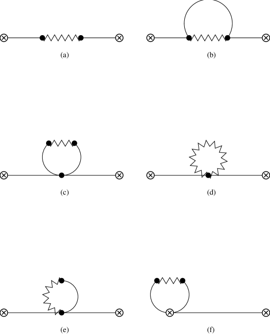
Figure 3: Chiral Perturbation Theory contributions to $\Pi_{\Delta S=a}(q^{2})$. (a) Lowest order. (b)-(f) Higher order non-factorizable. The full lines are mesons. The zig–zag line is the $X$-boson.

It turns out however that in the presence of a cut-off some of the contributions obtained with this routing do not have the correct CPS symmetry. This symmetry imposes that some of the contributions have to have the internal propagator in Fig. 3 with momentum $r+2q$ instead of $r$. The precise change has been depicted in Fig. 4. The momentum flow as depicted in (a) should be replaced by the sum of (b) and (c).

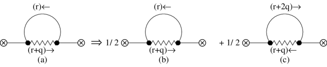
Figure 4: The routing for the $\Delta S=2$ operator enforced by CPS symmetry. (a) Routing used in [2], (b)+(c) The correct routing as it should have been used.

This doesn’t affect the coefficients of the chiral logarithms. Therefore one can use any routing when using regularization which doesn’t see analytic dependence on the cut-off. Unfortunately, this bad routing was actually causing most of the bad behaviour for $B_{K}(\mu)$ for high values of $\mu$ in Table 1 of [2] and the difference with the result for $G_{27}$ of [2] and [3]. In fact, using the background field method as in [3] the CPS symmetry is automatically satisfied at order $p^{2}$ with any routing.

We have now corrected for this problem and obtain a much more reasonable matching between long-distance contributions and the short-distance contributions. Nevertheless, it turns out that the range of values chosen for $\mu$ in [2] to make the predictions was not very much affected by the routing problem explained above. The results we now obtain are much more stable numerically and in the same ranges as the ones quoted in [2]. We also agree with the result in [3] for $G_{27}(\mu)$ obtained from lowest order CHPT,

$$G_{27}(\mu)=1-\frac{3\mu^{2}}{16\pi^{2}F_{0}^{2}}\,.$$ (28)

Here and in what follows, the $\mu$ dependent $G_{8}(\mu)$, $G_{8}^{\prime}(\mu)$, $G_{27}(\mu)$, and $B_{K}(\mu)$ couplings stand for the long-distance contributions to those couplings, i.e. with $[1+(\alpha_{s}(\mu)/\pi)\,r_{1,j}]\,C_{j}(\mu)=1$.

4.2 CHPT Results

Here we update Section 4 of [2] to correct for the routing problem. The non-factorizable contribution to $\Pi^{\overline{K}^{0}\,K^{0}}(q^{2})$ is given by the diagrams in Figure 3 and is:

$$\frac{-8B_{0}^{2}F_{0}^{2}}{(q^{2}-m_{K}^{2})^{2}}\Bigg{\{}\int^{\mu}\frac{d^{4}r_{E}}{(2\pi)^{4}}\frac{r_{E}^{2}q_{E}^{2}}{(r_{E}^{2}+m_{K}^{2})^{2}}-\int^{\mu}\frac{d^{4}r_{E}}{(2\pi)^{4}}\frac{r_{E}^{2}}{r_{E}^{2}+m_{K}^{2}}$$

$$\!\!\!+\frac{1}{2}\int^{\mu}\frac{d^{4}r_{E}}{(2\pi)^{4}}(r_{E}+2q_{E})^{2}\left[\frac{1}{(r_{E}+q_{E})^{2}+m_{\pi}^{2}}+\frac{1}{(r_{E}+q_{E})^{2}+2m_{K}^{2}-m_{\pi}^{2}}\right]\Bigg{\}}$$

These integrals can be performed analytically but the result is rather cumbersome. The Euclidean continuation of $q^{2}$ we used is $q_{E}^{2}=-q^{2}$. The result in the chiral limit becomes

$$\frac{-8B_{0}^{2}F_{0}^{2}}{(q^{2}-m_{K}^{2})^{2}}\frac{1}{16\pi^{2}F_{0}^{2}}\left\{-3\mu^{2}q^{2}-\frac{5}{6}q^{4}\right\}$$ (30)

and for $q^{2}$ = 0

$$\frac{-8B_{0}^{2}F_{0}^{2}}{(q^{2}-m_{K}^{2})^{2}}\frac{1}{16\pi^{2}F_{0}^{2}}$$

$$\times\Bigg{\{}-\frac{1}{2}(2m_{K}^{2}-m_{\pi}^{2})\left(\mu^{2}-(2m_{K}^{2}-m_{\pi}^{2})\ln\left(\frac{\mu^{2}+2m_{K}^{2}-m_{\pi}^{2}}{2m_{K}^{2}-m_{\pi}^{2}}\right)\right)$$

$$+m_{K}^{2}\left(\mu^{2}-m_{K}^{2}\ln\left(\frac{\mu^{2}+m_{K}^{2}}{m_{K}^{2}}\right)\right)-\frac{1}{2}m_{\pi}^{2}\left(\mu^{2}-m_{\pi}^{2}\ln\left(\frac{\mu^{2}+m_{\pi}^{2}}{m_{\pi}^{2}}\right)\right)\Bigg{\}}$$

These results allow to obtain the equivalent of (28) for the $O(p^{4})$ coefficients.

4.3 The $B_{K}$ Parameter: Long Distance and Short Distance

We now take the results from the ENJL evaluation of $\Pi^{\overline{K}^{0}\,K^{0}}(q^{2})$ both in the chiral limit and in the case of quark masses corresponding to the physical pion and kaon mass and use these to estimate $B_{K}$ and $G_{27}$.

The final results for $B_{K}$ in the chiral limit, $B_{K}^{\chi}(\mu)$ and $G_{27}(\mu)=4B_{K}^{\chi}(\mu)/3$ are shown in Table 1.

$\mu$(GeV)	$G_{27}(\mu)$	$B_{K}^{\chi}(\mu)$	$B_{K}(\mu)$	$\hat{B}_{K(1)}$	$\hat{B}_{K(2)}^{\mbox{SI}}$	$\hat{B}_{K(2)}^{\exp}$	$\hat{B}_{K(2)}^{\chi\exp}$
0.3	0.830	0.622	0.784	–	–	–	–
0.4	0.737	0.552	0.776	–	–	–	–
0.5	0.638	0.478	0.762	0.79	0.36	0.48	0.30
0.6	0.537	0.402	0.746	0.81	0.57	0.62	0.33
0.7	0.431	0.323	0.721	0.81	0.63	0.66	0.30
0.8	0.320	0.240	0.688	0.79	0.65	0.67	0.23
0.9	0.200	0.150	0.643	0.75	0.64	0.66	0.15
1.0	0.070	0.052	0.588	0.70	0.61	0.62	0.05

Table 1: The long-distance contributions to $G_{27}(\mu)$, $B_{K}^{\chi}(\mu)$ and $B_{K}(\mu)$ as determined using the ENJL model. Also shown are $\hat{B}_{K(1)}$ using the one-loop short distance and $\hat{B}_{K(2)}$, $\hat{B}_{K(2)}^{\chi}$ using the two-loop short distance in Table 7. See Appendix A for the values of the parameters used. For the non-chiral cases one has to add 0.09$\pm$0.03 from the nonet vs octet difference, see text.

We have also shown the value of $B_{K}$ obtained there from extrapolating the ENJL two-point function in the Euclidean domain to the kaon pole using Chiral Perturbation Theory, this is $B_{K}(\mu)$. In the latter case we have to include the correction due to the difference between the octet and nonet case. This correction was estimated to be about $0.09\pm 0.03$ in [2] and we take it as $\mu$-independent. In the other columns in Table 1 various parts of the short distance correction are included. The realistic case, with non-zero quark masses in the long distance contribution to $B_{K}(\mu)$, we have shown with the one-loop short-distance running, $\hat{B}_{K(1)}$, two-loop short distance running with the scheme-dependence removed, $\hat{B}^{SI}_{K(2)}$, as defined in eq. (69), and the exact solution to the two-loop evolution equation with the scheme-dependence removed to the same order, $\hat{B}^{exp}_{K(2)}$ as defined in Eq. (70). For the latter short-distance contribution we have also shown the result in the chiral limit, $\hat{B}_{K(2)}^{\chi exp}$. The rest of the parameters used are in App. A. Notice that the matching for all cases is acceptable. The quality of the matching for the real $\hat{B}_{K}$ is as good as for $\hat{B}^{exp}_{K(2)}$ since they only differ by the $\mu$-independent correction of 0.09 described above.

So, in the chiral limit we get

$$0.25<\hat{B}_{K}^{\chi}<0.40\,,$$ (32)

with non-zero quark masses we get

$$0.50<\hat{B}_{K}^{\rm Nonet}<0.70$$ (33)

for the nonet case and

$$0.59<\hat{B}_{K}<0.79$$ (34)

for the real case. Notice that the large value of the chiral symmetry breaking ratio

$$1.8<\frac{B_{K}}{B_{K}^{\chi}}<2.4\,$$ (35)

confirms the qualitative picture obtained in [2]. Finally, let us split the different contributions to the value of $\hat{B}_{K}$ in the real case,

$$\hat{B}_{K}=(0.33\pm 0.10)+(0.09\pm 0.02)+(0.18\pm 0.07)+(0.09\pm 0.03)$$ (36)

where the first terms is the chiral limit result, the second term are the $O(p^{4})$ chiral logs at $\nu=M_{\rho}$ [2], the third term are the $O(p^{4})$ counterterms and higher also at the same scale and the last term is the above mentioned contribution due to the $\eta_{1}-\eta_{8}$ mixing [2]. The error on the chiral log contribution is from varying $\nu$ and the one on the counterterm contribution from looking at various different ways to extract the same counterterms as described in [2] plus some extra as an estimate of the model error.

Notice that the last term in (36) is of order $(m_{s}-m_{d})/N_{c}^{2}$ and it is not included in present lattice results. In fact, it introduces an unknown systematic uncertainty in quenched and partially unquenched results which is difficult to pin down, see [11]. So the lattice results cannot be easily compared to ours. This term is also not included in determinations which are based in lowest order CHPT since it is higher order. Therefore again a direct comparison with our results has to be done carefully.

5 $\Delta S=1$ Transitions: Long Distance

In this section we use the $\Delta S=1$ two-point-functions $\Pi^{K^{+}\pi^{+}}(q^{2})$ and $\Pi^{K^{0}\pi^{0}}(q^{2})$ as defined in (14). We do not use the one with $\eta_{8}$ since to order $p^{2}$ we do not get any more information out of that two-point function. It will provide extra information to $O(p^{4})$ [12]. The result to lowest order in CHPT is given by

$$\!\!\Pi^{K^{+}\pi^{+}}(q^{2}) = -\frac{4B_{0}^{2}F_{0}^{4}\,C}{(q^{2}-m_{K}^{2})(q^{2}-m_{\pi}^{2})}\left[q^{2}\left(G_{8}+\frac{2}{3}G_{27}-2G_{8}^{\prime}\right)+m_{\pi}^{2}G_{8}^{\prime}\right]$$

$$\hskip-0.85358pt\Pi^{K^{0}\pi^{0}}(q^{2}) = -\frac{2\sqrt{2}B_{0}^{2}F_{0}^{4}\,C}{(q^{2}-m_{K}^{2})(q^{2}-m_{\pi}^{2})}\left[q^{2}\left(-G_{8}+G_{27}+2G_{8}^{\prime}\right)-m_{\pi}^{2}G_{8}^{\prime}\right]$$ (37)

Here $C$ of Eq. (7) has been chosen such that in the strict large-$N_{c}$ limit $G_{8}=G_{27}=1$. The coupling $G_{8}^{\prime}$ is the coefficient of the weak mass term that does not contribute to $K\to\pi\pi$ at order $p^{2}$ but its value is important at $O(p^{4})$ and higher and for some processes involving photons. The definition of the $O(p^{2})$ Lagrangian, a discussion of the contributions from $G_{8}^{\prime}$ and further references can be found in [12].

We have calculated the two-point functions in the chiral limit to extract the coefficient of $q^{2}$ and in the case of equal quark masses for an ENJL quark mass of 0.5, 1, 5, 10, and 20 MeV in order to extract the coefficient of $m_{\pi}^{2}$.

As described in Section 3.2 we treat all coefficients $C_{i}(\mu_{L})$ as leading order in $1/N_{c}$ since they are enhanced in principle by large logarithms. We therefore obtain the matrix elements of $Q_{1}$, $Q_{2}$, $Q_{3}$, $Q_{4}=Q_{2}-Q_{1}+Q_{3}$, $Q_{5}$ and $Q_{6}$ to next-to-leading order in $1/N_{c}$.

5.1 Current x Current Operators

The comments here are only valid for $Q_{1},Q_{2},Q_{3},Q_{4}$, and $Q_{5}$. The operator $Q_{6}$ is special and is treated separately in the next subsection.

We can now use the method of [9] with the correct routing and obtain for the contributions to $G_{8}$ and $G_{8}^{\prime}$ from $Q_{1}$, $Q_{2}$, $Q_{3}$ and $Q_{5}$ [with $\Delta_{\mu}\equiv\mu^{2}/(16\pi^{2}F_{0}^{2})$]:

$$G_{27}(\mu)[Q_{1}] = G_{27}(\mu)[Q_{2}]=1-3\Delta_{\mu}+O(p^{4})\,,$$

$$G_{8}(\mu)[Q_{1}] = -\frac{2}{3}\left[1+\frac{9}{2}\Delta_{\mu}+O(p^{4})\right]\,,$$

$$G_{8}(\mu)[Q_{2}] = 1+\frac{9}{2}\,\Delta_{\mu}+O(p^{4})\,,$$

$$G_{8}(\mu)[Q_{3}] = 2G_{8}(\mu)[Q_{2}]+3G_{8}(\mu)[Q_{1}]=0+O(p^{4})\,,$$

$$G_{8}(\mu)[Q_{5}] = 0+O(p^{4})\,,$$

$$G_{8}^{\prime}(\mu)[Q_{1}] = 0\,,$$

$$G_{8}^{\prime}(\mu)[Q_{2}] = \frac{5}{6}\,\Delta_{\mu}+O(p^{4})\,,$$

$$G_{8}^{\prime}(\mu)[Q_{3}] = 2G_{8}^{\prime}(\mu)[Q_{2}]=\frac{5}{3}\,\Delta_{\mu}+O(p^{4})\,,$$

$$G_{8}^{\prime}(\mu)[Q_{5}] = -\frac{5}{3}\Delta_{\mu}+O(p^{4})\,.$$ (38)

Here and in the remainder $G_{8}(\mu)[Q_{i}]$ stands for the long-distance contribution of operator $Q_{i}$ to $G_{8}$ when $C_{i}(\mu)$ is set equal to 1. The same definition applies to $G_{8}^{\prime}(\mu)[Q_{i}]$ and $G_{27}(\mu)[Q_{i}]$. In Tables 2 and 3 we dropped the argument $(\mu)$ for brevity. The results from the ENJL calculations are summarized in Table 2. The numbers in the columns 2 to 8 are always assuming $[1+(\alpha_{s}(\mu)/\pi)\,r_{1,j}]\,C_{j}(\mu)=1$ for the relevant operator.

We get that $G_{27}(\mu)[Q_{1}]=G_{27}(\mu)[Q_{2}]=G_{27}(\mu)$ in Table 1 and they are therefore not listed again. In addition all the other operators are octet so do not contribute to $G_{27}$. We also have $G_{8}^{\prime}(\mu)[Q_{1}]=0$, the operator $Q_{1}$ only contributes via $B_{K}$-like contributions which cannot have a contribution at $q^{2}=0$ for equal quark masses since this type of contribution also produces $G_{27}$ where such terms are forbidden. The approach to the chiral limit for the left-left current operators $Q_{1}$, $Q_{2}$, and $Q_{3}$ is such that the $B_{K}$-like and Penguin-like contributions are separately chiral invariant. For the left-right current operator $Q_{5}$ this is not the case and it is only the sum of the $B_{K}$-like and Penguin-like contributions that vanishes for $q^{2}\to 0$ in the chiral limit. Notice that the results for small $\mu$ agree quite well with the results just using CHPT, eq. (5.1), but differ strongly for larger $\mu$. The values (5.1) at $\mu=0$ correspond to the factorizable contribution.

We have also calculated the chiral logarithms that should be present in these contributions. Subtracting them made the extraction of the coefficient of $m_{\pi}^{2}$ to obtain $G_{8}^{\prime}$ numerically much more convergent.

$\mu$ (GeV)	$G_{8}[Q_{1}]$	$G_{8}[Q_{2}]$	$G_{8}[Q_{3}]$	$G_{8}[Q_{5}]$	$G_{8}^{\prime}[Q_{2}]$	$G_{8}^{\prime}[Q_{3}]$	$G_{8}^{\prime}[Q_{5}]$
0.0	-0.667	1.000	0.000	0.000	0.000	0.000	0.000
0.3	-0.834	1.271	0.040	-0.041	0.070	0.140	-0.149
0.4	-0.930	1.425	0.060	-0.109	0.128	0.256	-0.297
0.5	-1.029	1.600	0.113	-0.244	0.206	0.412	-0.530
0.6	-1.130	1.779	0.168	-0.460	0.298	0.596	-0.868
0.7	-1.235	1.962	0.219	-0.769	0.399	0.798	-1.321
0.8	-1.347	2.145	0.249	-1.178	0.501	1.002	-1.908
0.9	-1.467	2.325	0.249	-1.690	0.598	1.196	-2.634
1.0	-1.597	2.498	0.205	-2.308	0.681	1.362	-3.504

Table 2: The results for the long-distance contributions to $G_{8}(\mu)$ and $G_{8}^{\prime}(\mu)$ from $Q_{1}$ to $Q_{5}$ $[Q_{4}=Q_{2}-Q_{1}+Q_{3}]$ as calculated using the ENJL model via the two-point functions.

The results for $G_{8}(\mu)[Q_{3}]$ can be obtained from isospin relations from $G_{8}(\mu)[Q_{1}]$ and $G_{8}(\mu)[Q_{2}]$. The results for $G_{8}(\mu)[Q_{5}]$ come from a large cancellation between the values of $G_{8}-2G_{8}^{\prime}$ and $G_{8}^{\prime}$ and have a somewhat larger uncertainty than the others.

It should be noticed that in all cases the $1/N_{c}$ corrections to the matrix elements are substantial.

5.2 The $Q_{6}$ Operator: Factorization Problem and Results

After Fierzing, the $Q_{6}$ operator defined in (3.1)

$$Q_{6} \equiv -2{\displaystyle\sum_{q=u,d,s}}\,\left[\overline{s}\,(1+\gamma_{5})\,q\right](x)\,\left[\overline{q}\,(1-\gamma_{5})\,d\right](x)$$ (39)

gives both factorizable and non-factorizable contributions to the off-shell two-point functions to $K^{0}\to\pi^{0}$, $K^{0}\to\eta_{8}$, and $K^{+}\to\pi^{+}$. Here, we study for definiteness the $K^{+}\to\pi^{+}$ two-point function, $\Pi^{K^{+}\pi^{+}}(q^{2})$ of Eq. (14). The factorizable contributions from $Q_{6}$ to this two-point function are

$$\Pi^{K^{+}\pi^{+}}_{Q_{6}Fact}(q) = 2C_{\Delta S=1}\,C_{6}(\mu)\left[\langle 0|\overline{d}d+\overline{s}s|0\rangle\,\,\Pi^{P_{K^{-}}S_{32}P_{\pi^{+}}}(0,q)\right.$$ (40)

$$- \left.\Pi^{P}_{K^{+}K^{+}}(q)\,\Pi^{P}_{\pi^{+}\pi^{+}}(q)\,\right].$$

Here $C_{6}(\mu)$ is the Wilson coefficient of $Q_{6}$, $\Pi_{P}^{ii}(q)$ are two-point functions

$$\Pi_{P}^{ii}(q)\equiv i\int{\rm d}^{4}x\,e^{iq.x}\,\langle 0|T(P_{i}^{\dagger}(0)P_{i}(x))|0\rangle=-\left[\frac{Z_{i}}{q^{2}-m_{i}^{2}}+Z^{\prime}_{i}\right],$$ (41)

with $P_{i}(x)$ the pseudo-scalar sources defined in (3.1), and $\Pi^{P_{K^{-}}S_{32}P_{\pi^{+}}}(p,q)$ the three-point function

$$\Pi^{P_{K^{-}}S_{32}P_{\pi^{+}}}(p,q) \equiv i^{2}\int{\rm d}^{4}x\,\int{\rm d}^{4}y\,e^{i(q.x-p.y)}\,\langle 0|T(P_{K^{-}}(x)S_{32}(y)P_{\pi^{+}}(0))|0\rangle$$

with $S_{32}(y)$ the scalar source

$$S_{32}(y)\equiv-\left[\overline{s}\,d\right](y)\,.$$ (43)

The last term in Eq. (40) corresponds to the diagram shown in Fig. 1(a). The first term is a contribution which is absent in the case of current$\times$current operators. It is depicted in Fig. 5.

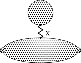
Figure 5: The factorizable contribution for the $Q_{6}$ operator that is not well defined in the chiral limit. This contribution is not present for current$\times$current operators.

In octet symmetry, to next-to-leading order we have [28]

$$\frac{\displaystyle\langle 0|\overline{d}d+\overline{s}s|0\rangle}{-2B_{0}F_{0}^{2}}=1+\frac{16}{F_{0}^{2}}\,(2m_{K}^{2}+m_{\pi}^{2})L_{6}+\frac{4}{F_{0}^{2}}\,m_{K}^{2}\,(2L_{8}+H_{2})-\frac{3}{2}\mu_{\pi}-3\mu_{K}-\frac{5}{6}\mu_{\eta_{8}}$$ (44)

for the one-point function and

$$\Pi^{P_{K^{-}}S_{32}P_{\pi^{+}}}(0,q)=-\frac{\sqrt{Z_{K^{+}}Z_{\pi^{+}}}}{(q^{2}-m_{K}^{2})(q^{2}-m_{\pi}^{2})}\,B_{0}$$ (45)

$$\times \left[1+\frac{8}{F_{0}^{2}}\,(2m_{K}^{2}+m_{\pi}^{2})(2L_{6}-L_{4})\right.-\frac{4}{F_{0}^{2}}\,(2q^{2}+m_{K}^{2}+m_{\pi}^{2})\,L_{5}+\frac{32}{F_{0}^{2}}\,q^{2}\,L_{8}$$

$$\!\!\!\!\!\!\!-{1\over 6}\frac{q^{2}}{16\pi^{2}F_{0}^{2}}\left[\ln\left(\frac{m_{K}^{2}}{\nu^{2}}\right)-{3\over 2(m_{K}^{2}-m_{\pi}^{2})}\left(m_{\pi}^{2}\ln\left({m_{\pi}^{2}\over m_{K}^{2}}\right)+m_{\eta_{8}}^{2}\ln\left({m_{\eta_{8}}^{2}\over m_{K}^{2}}\right)\right)\right]$$

$$+{1\over 2}\mu_{\pi}+{1\over 6}\mu_{\eta_{8}}+{5\over 6}\mu_{K}+\frac{5}{12}\,\frac{m_{\pi}^{2}}{16\pi^{2}F_{0}^{2}}\ln\left(\frac{m_{K}^{2}}{\nu^{2}}\right)$$

$$-\left.\frac{m_{K}^{2}+m_{\pi}^{2}}{16\pi^{2}F_{0}^{2}}\,{1\over 8(m_{K}^{2}-m_{\pi}^{2})}\left[m_{\eta_{8}}^{2}\ln\left({m_{\eta_{8}}^{2}\over m_{K}^{2}}\right)-3m_{\pi}^{2}\ln\left({m_{\pi}^{2}\over m_{K}^{2}}\right)\right]\right]$$

for the three-point function. Here and in the remainder the constants $L_{i}$ are defined at a scale $\nu$, $L_{i}\equiv L_{i}^{r}(\nu)$. and $\mu_{i}=\ln(m_{i}/\nu)/(16\pi^{2})$ for $i=\pi,K,\eta_{8}$.

At next-to-leading order, the expressions for the two-point functions were given for the octet symmetry case in [12]. So the second part in (40) can be written as

$$\Pi^{P}_{K^{+}K^{+}}(q)\,\Pi^{P}_{\pi^{+}\pi^{+}}(q)=\frac{\sqrt{Z_{K^{+}}Z_{\pi^{+}}}}{(q^{2}-m_{K}^{2})(q^{2}-m_{\pi}^{2})}\,2F_{0}^{2}B_{0}^{2}$$ (46)

$$\times \left[1+\frac{8}{F_{0}^{2}}(2m_{K}^{2}+m_{\pi}^{2})(4L_{6}-L_{4})\right.+\frac{4}{F_{0}^{2}}(m_{\pi}^{2}+m_{K}^{2})(4L_{8}-L_{5})$$

$$+\frac{4}{F_{0}^{2}}(2q^{2}-m_{\pi}^{2}-m_{K}^{2})(2L_{8}-H_{2})-\left.\frac{7}{4}\mu_{\pi}-\frac{5}{2}\mu_{K}-\frac{5}{12}\mu_{\eta_{8}}\right]$$

Therefore this order, in octet symmetry, the factorizable contributions to $\Pi^{K^{+}\pi^{+}}(q)$ from $Q_{6}$ are

$$\Pi^{K^{+}\pi^{+}}_{Q_{6},Fact}(q)=-\frac{\sqrt{Z_{K^{+}}Z_{\pi^{+}}}}{(q^{2}-m_{K}^{2})(q^{2}-m_{\pi}^{2})}\,C_{\Delta S=1}\,C_{6}(\mu)\,16B_{0}^{2}(\mu)$$ (47)

$$\times \Bigg{\{}2q^{2}\left\{L_{5}-(2L_{8}+H_{2})\right\}+m_{\pi}^{2}(2L_{8}+H_{2})-{1\over 12}\mu_{K}+{1\over 16}\mu_{\eta_{8}}-{3\over 16}\mu_{\pi}$$

$$\hskip-22.76228pt+{1\over 24}\frac{q^{2}}{16\pi^{2}F_{0}^{2}}\left[\ln\left(\frac{m_{K}^{2}}{\nu^{2}}\right)-{3\over 2(m_{K}^{2}-m_{\pi}^{2})}\left(m_{\pi}^{2}\ln\left({m_{\pi}^{2}\over m_{K}^{2}}\right)+m_{\eta_{8}}^{2}\ln\left({m_{\eta_{8}}^{2}\over m_{K}^{2}}\right)\right)\right]$$

$$-\frac{5}{48}\,\frac{m_{\pi}^{2}}{16\pi^{2}F_{0}^{2}}\ln\left(\frac{m_{K}^{2}}{\nu^{2}}\right)$$

$$+\frac{m_{K}^{2}+m_{\pi}^{2}}{16\pi^{2}F_{0}^{2}}\,{1\over 32(m_{K}^{2}-m_{\pi}^{2})}\left[m_{\eta_{8}}^{2}\ln\left({m_{\eta_{8}}^{2}\over m_{K}^{2}}\right)-3m_{\pi}^{2}\ln\left({m_{\pi}^{2}\over m_{K}^{2}}\right)\right]\Bigg{\}}$$

As it is well known the order $p^{0}$ contribution from $Q_{6}$ vanishes [29] and the first non-trivial contribution from this operator is of order   $p^{2}$. This happens here as an exact cancellation between the two types of factorizable contributions at order $p^{0}$. As a result there is a very large cancellation between the two types of factorizable contributions at order $p^{2}$. We get

$$G_{8}\Bigg{|}_{Q_{6},\mbox{Fact}}=-\left[{5\over 3}\right]\,16\,C_{6}(\mu)\frac{B_{0}^{2}(\mu)}{F_{0}^{2}}\,\left[L_{5}-{3\over 16}\frac{1}{16\pi^{2}}\left[2\ln\left(\frac{m_{L}}{\nu}\right)+1\right]\right]\\$$

and

$$G_{8}^{\prime}\Bigg{|}_{Q_{6},\mbox{Fact}}=-\left[{5\over 3}\right]\,8\,C_{6}(\mu)\frac{B_{0}^{2}(\mu)}{F_{0}^{2}}\,\left[(2L_{8}+H_{2})-\frac{5}{24}\,\frac{1}{16\pi^{2}}\left[2\ln\left(\frac{m_{L}}{\nu}\right)+1\right]\right]$$ (48)

The mass $m_{L}$ above has to be understood as an infrared cut-off as we have done the chiral limit $m_{L}=m_{\pi}=m_{K}=m_{\eta_{8}}\to 0$. The factorizable contribution to $G_{8}$ and G${}_{8}^{\prime}$ from $Q_{6}$ is therefore not well defined. It has an infrared divergence. The divergence is related to the divergence in the pion scalar radius in the chiral limit. Since $Q_{6}$ is an $8_{L}\times 1_{R}$ operator we know from CHPT in the non-leptonic sector that to lowest order in the counting there, no infrared divergences are present in the two-point function $\Pi^{K^{+}\pi^{+}}(q^{2})$. These infrared divergences are therefore spurious and must be cancelled by another contribution. The only possibility is that it cancels out with the non-factorizable contribution also coming from $Q_{6}$. We will see below that this is indeed the case. Notice also that since $G_{8}$ and $G_{8}^{\prime}$ are $O(p^{2})$ couplings, Eqs. (5.2) and (48) are exact for the factorizable contributions.

Unfortunately, the non-factorizable contributions can only be calculated at present in a model dependent way. In the $1/N_{c}$ expansion, the infrared divergent part of $G_{8}$ and $G_{8}^{\prime}$ can in fact be calculated analytically using the $O(p^{2})$ CHPT Lagrangian. We can therefore subtract it. It follows from the diagrams shown in Fig. 3, (b),(c), (e), and (f) and by using CHPT for the $X$-boson vertices which is valid for small $\mu$. For equal masses $m_{K}^{2}=m_{\pi}^{2}=m_{\eta_{8}}^{2}=m_{L}^{2}$ we obtain

$$\Pi^{K^{+}\pi^{+}}(q^{2})=\frac{2B_{0}^{2}F_{0}^{2}}{(q^{2}-m_{K}^{2})(q^{2}-m_{\pi}^{2})}C_{\Delta S=1}C_{6}(\mu)4B_{0}^{2}(\mu)$$

$$\times \Bigg{\{}-\frac{1}{6}(q^{2}-5m_{L}^{2})\int^{\mu}\frac{d^{4}r_{E}}{(2\pi)^{4}}\frac{1}{(r_{E}^{2}+m_{L}^{2})^{2}}$$

$$-\frac{5}{6}\int^{\mu}\frac{d^{4}r_{E}}{(2\pi)^{4}}\left[\frac{1}{((r_{E}+q_{E})^{2}+m_{L}^{2})}-\frac{1}{(r_{E}^{2}+m_{L}^{2})}\right]\Bigg{\}}\,.$$

The non-factorizable (NF) part above in the limit $m_{L}\to 0$ leads to

$$G_{8}{\Bigg{|}_{\mbox{$Q_{6}$,NF-$O(p^{2})$}}}=-\left[{5\over 3}\right]\,16\,C_{6}(\mu)\frac{B_{0}^{2}(\mu)}{F_{0}^{2}}\,\frac{3}{16}\,\frac{1}{16\pi^{2}}\left[2\ln\left(\frac{m_{L}}{\mu}\right)+\frac{13}{18}\right]$$ (50)

and

$$G_{8}^{\prime}{\Bigg{|}_{\mbox{$Q_{6}$,NF-$O(p^{2})$}}}=-\left[{5\over 3}\right]\,8\,C_{6}(\mu)\frac{B_{0}^{2}(\mu)}{F_{0}^{2}}\,\frac{5}{24}\,\frac{1}{16\pi^{2}}\left[2\ln\left(\frac{m_{L}}{\mu}\right)+1\right]$$ (51)

There is a very large cancellation between the factorizable parts in (5.2) and (48) and the non-factorizable part in (50) and (51) both for the IR divergent part and for the large $1/N_{c}$ constant part. Summing up the exact factorizable result and the infrared divergent non-factorizable part we get

$$G_{8}\Bigg{|}_{\mbox{$Q_{6}$, $O(p^{2})$}}=-\left[{5\over 3}\right]\,16\,C_{6}(\mu)\frac{B_{0}^{2}(\mu)}{F_{0}^{2}}\,\left[L_{5}(\nu)-\frac{1}{16\pi^{2}}\left({3\over 8}\ln\left(\frac{\mu}{\nu}\right)+\frac{5}{96}\right)\right]$$ (52)

and

$$G_{8}^{\prime}\Bigg{|}_{\mbox{$Q_{6}$, $O(p^{2})$}}=-\left[{5\over 3}\right]\,8\,C_{6}(\mu)\frac{B_{0}^{2}(\mu)}{F_{0}^{2}}\,\left[(2L_{8}+H_{2})(\nu)-\frac{5}{12}\,\frac{1}{16\pi^{2}}\ln\left(\frac{\mu}{\nu}\right)\right]$$ (53)

It is then a non-trivial check of the validity of the model used that the non-factorizable part indeed contains the correct infrared logarithms needed to cancel the factorizable ones. The ENJL model used here does.

Notice in (52) and (53) all the dependence on the IR scale , $m_{L}^{2}$, drops out as it should and the scale in the logarithm becomes $\ln(\mu/\nu)$. So in the chiral limit and next-to-leading in $1/N_{c}$ , the scale dependence on the short-distance scale gets compared to the scale where the CHPT constants are defined.

The result above shows that at least the $B_{6}$ parameter defined as usual as the ratio of the non-factorizable contributions over the vacuum saturation result (VSA) is not well defined. It is therefore necessary to give another definition for this $B$ parameter. The cancellation of the infrared divergence found here is probably also the source for the large cancellations found between the factorizable and non-factorizable contributions in earlier work. Notice also that the $1/N_{c}$ finite term in (5.2) is larger than the leading in $1/N_{c}$ result and with opposite sign. It is clear that it can be dangerous not to have and analytical cancellation of both the IR divergent part and the $1/N_{c}$ constant as we have. This can explain also some discrepancies for the $B_{6}$ parameter results in the literature, $B_{6}$ is just not well defined.

The way we treat our results is that we remove the exact infrared logarithm from our ENJL calculation by adding equations (5.2) and (48) which are exact and model independent to the ENJL results. In this way we also remove the IR divergence of the non-factorizable part exactly. We chose the reference scale $\mu=M_{\rho}$ to do the subtraction. We generate the mass $m_{L}^{2}$ by putting small current quark masses. The remaining factorizable factor, i.e. the part from the constants $L_{5}$, $L_{8}$, and $H_{2}$ are then evaluated at a scale $\nu=M_{\rho}$. This corresponds for the leading in $1/N_{c}$ contribution to $G_{8}$ and $G_{8}^{\prime}$ from $Q_{6}$

$$G_{8}^{ENJL}{\Bigg{|}_{\mbox{$N_{c}$}}}=(-38\pm 8)\,C_{6}(\mu)\quad{\rm and}\quad G_{8}^{\prime ENJL}{\Bigg{|}_{\mbox{$N_{c}$}}}=(-9\pm 14)\,C_{6}(\mu)$$ (54)

using

$$L_{5}(M_{\rho}) = (1.4\pm 0.3)\cdot 10^{-3}$$

$$(2L_{8}+H_{2})(M_{\rho}) = (0.7\pm 1.1)\cdot 10^{-3}\,.$$ (55)

We have used here the value of $B_{0}$ and $F_{0}$ from the ENJL model. The value of $2L_{8}+H_{2}$ is derived from the canonical value for $L_{8}(M_{\rho})=(0.9\pm 0.3)\cdot 10^{-3}$ and the value for $(2L_{8}-H_{2})(M_{\rho})=(2.9\pm 1.0)\cdot 10^{-3}$ from [33]. The large error for $G_{8}^{{}^{\prime}ENJL}$ in (54) is because of the large cancellation in the value for $2L_{8}+H_{2}$. Notice that the size of the subtracted terms in $G_{8}^{ENJL}$ is about $+40\,C_{6}(\mu)$ for $m_{L}^{2}=m_{\pi}m_{K}$ and varies very fast with $m_{L}$.

Our calculation agrees with the one of [30] when the appropriate identifications are made. The large cancellation between the factorizable and non-factorizable parts where also observed there. They were however not identified as an exact cancellation of infrared divergences. In fact, at the order the calculation was done in [30] the cancellation of the $1/N_{c}$ factorizable and non-factorizable pieces is very large, and in their language one should get $B_{6}$ very near to one. They get indeed $B_{6}$ very close to one.

The non-factorizable non-divergent part has corrections from higher order terms in the chiral Lagrangian which we calculate numerically using the ENJL model. We have included them and these give therefore the numerical differences between our results and the ones in [30].

Before we present the results for $G_{8}(\mu)$ and $G_{8}^{\prime}(\mu)$ from $Q_{6}$ from our ENJL calculation we need to include one additional remark. The vector and axial-vector currents used in the previous section are uniquely identified both in the ENJL model and in QCD. There is however no guarantee as remarked in [23] that the same is true for the scalar and pseudo-scalar densities. Here we renormalize the ENJL scalar $S(x)$ and pseudo-scalar $P(x)$ densities by the values of the quark condensates in the chiral limit:

$$S_{\mbox{ENJL}}=S_{\mbox{QCD}}(\mu)\frac{\langle\bar{q}q\rangle_{\mbox{ENJL}}}{\langle\bar{q}q\rangle_{\mbox{QCD}}(\mu)}.$$ (56)

There is an analogous equation for the pseudo-scalar density. This factor should be remembered when using the Wilson coefficients from our results. The values we have used are $B_{0}^{QCD}(1{\rm GeV})=(1.75\pm 0.40)$ GeV in the $\overline{MS}$ scheme [33, 34], and $B_{0}^{ENJL}=2.80$ GeV [21]. We have also included the QCD scale dependence of the $B_{0}$ parameter to two-loops. We show in Table 3 the results for $G_{8}(\mu)[Q_{6}]$ and $G_{8}^{\prime}(\mu)[Q_{6}]$ without the renormalization factor of Eq. (56), columns labelled ENJL, and including the renormalization factor of Eq. (56) both to one-loop, columns labelled ⁽¹⁾, and two-loops in QCD , columns labelled ⁽²⁾. Notice $B_{0}(\mu)=-\langle\bar{q}q\rangle(\mu)/F_{0}^{2}$ and this factor is responsible for most of the running of $Q_{6}$[31].

$\mu$ (GeV)	$G_{8}[Q_{6}]$	$G_{8}^{\prime}[Q_{6}]$	$G_{8}[Q_{6}]$	$G_{8}^{\prime}[Q_{6}]$	$G_{8}[Q_{6}]$	$G_{8}^{\prime}[Q_{6}]$
	ENJL	ENJL	(1)	(1)	(2)	(2)
0.3	-118	-69
0.4	-103	-53
0.5	-93	-41	-21.1	-9.3	-6.4	-2.8
0.6	-88	-32	-23.9	-8.7	-14.7	-5.3
0.7	-84	-25	-25.9	-7.7	-20.1	-6.0
0.8	-82	-20	-27.9	-6.8	-24.5	-6.0
0.9	-82	-17	-30.0	-6.2	-28.4	-5.9
1.0	-83	-15	-32.4	-5.9	-32.4	-5.9

Table 3: Results for the long-distance contributions to $G_{8}$ and $G_{8}^{\prime}$ from $Q_{6}$ as calculated using the ENJL model via the two-point functions for the non-factorizable part and adding the model independent factorizable part in (5.2) and (48). The last 4 columns include the renormalization of scalar and pseudo-scalar densities to one-loop ⁽¹⁾ and two-loops ⁽²⁾ in QCD. The short-distance anomalous dimensions for $B_{0}(\mu)$ at scales below 0.5 GeV blows up.

6 The Order $p^{2}$ Full $\Delta S=1$ Couplings

We use here the results of [7] and [6] for the $\Delta S=1$ QCD anomalous dimensions to one- and two-loops respectively to obtain final values. The solution for the Wilson coefficients are given in [7, 19] at two-loops using an expansion in $\alpha_{s}$. Whenever the values of $\Lambda_{QCD}$ are needed in the $\overline{MS}$ scheme with three flavours we use the expanded in $\alpha_{s}$ formulae [5] from $\alpha_{s}(M_{\tau})=0.334\pm 0.006$ with $M_{\tau}=1.77705\pm 0.00030$ GeV [5] and get $\Lambda^{(1)}_{QCD}=$ 220 MeV to one-loop and $\Lambda^{(2)}_{QCD}=$ 400 MeV to two-loops. The values of the Wilson coefficients we use for $\Delta S=1$ [7, 19] and for $\Delta S=2$ [32] are in the Appendix. We also include there the scheme dependent constants $r_{1}$ needed for the two-loops short-distance running in the NDR scheme we use.

We now show in Tables 4 and 5 the results for the coefficients $G_{27}$, $G_{8}$ and $G_{8}^{\prime}$. The numbers in brackets refer to keeping only $Q_{1}$, $Q_{2}$, and $Q_{6}$. Most of the difference is due to $Q_{4}$.

The matching for the one-loop running of the Wilson coefficients is very good. We obtain a value of $G_{8}\approx 4.3$ and $G_{8}^{\prime}\approx 0.8$. If we look inside the numbers, for $G_{8}$ the contribution via $Q_{1}$ is fairly constant over the whole range but there is a distinct shift from $Q_{2}$ to $Q_{6}$ for lower values of $\mu$. The operator $Q_{2}$ remains the most important over the entire range of $\mu$ considered. For $G_{8}^{\prime}$ similar comments apply except that $Q_{1}$ doesn’t contribute. Typically $G_{27}$ is somewhat low compared to the experimental number and we have not as good matching as in the octet sector. Notice though that it gets somewhat more stable in the range between 0.5 and 0.8 GeV as one expects from the validity of the low-energy model.

When two-loop running is taken into account in the NDR scheme the numbers do not change so much. The effect of the $r_{1}$ constants in this scheme is however very large and causes a significant shift in the numbers.

The numbers for the octet case are somewhat stable in the range $\mu=0.8$ to $1.0$ GeV but there is where the ENJL model is expected to start deviating from the true behaviour.

$\mu$ (GeV)	$G_{27}$	$G_{8}$	$G_{8}^{\prime}$
0.5	0.399	4.45 (4.55)	0.739 (0.761)
0.6	0.351	4.26 (4.34)	0.686 (0.710)
0.7	0.291	4.21 (4.28)	0.703 (0.727)
0.8	0.221	4.25 (4.30)	0.767 (0.789)
0.9	0.141	4.33 (4.37)	0.847 (0.866)
1.0	0.050	4.44 (4.46)	0.923 (0.935)

Table 4: The final results for the three $O(p^{2})$ couplings using the one-loop Wilson coefficients. The numbers in brackets refer to using $Q_{1}$, $Q_{2}$, and $Q_{6}$ only.

$\mu$ (GeV)	$G_{27}$	$G_{8}$	$G_{8}^{\prime}$
0.5	0.182	11.20 (12.4)	1.60 (1.75)
0.6	0.249	7.30 (7.8)	1.13 (1.22)
0.7	0.230	6.30 (6.6)	0.99 (1.10)
0.8	0.184	5.88 (6.2)	0.97 (1.08)
0.9	0.121	5.73 (5.9)	0.99 (1.11)
1.0	0.044	5.61 (5.8)	1.03 (1.14)

Table 5: The final results for the three $O(p^{2})$ couplings using the two-loop Wilson coefficients with the inclusion of the $r_{1}$ factors. The numbers in brackets refer to using $Q_{1}$, $Q_{2}$, and $Q_{6}$ only.

Notice that at large $N_{c}$, $G_{8}$ and $G_{27}$ are both 1. Adding $1/N_{c}$ corrections $G_{27}$ decreases by a non-negligible factor around two to three, while the $G_{8}$ coupling gets enhanced up to $G_{8}=6.2\pm 0.7$. The short-distance enhancement is almost a factor of two for the whole range of $\mu$. The rest of the enhancement, namely a factor two to three is mainly due to the large value of the long-distance contribution to the Penguin-like coupling $c$. The bulk of the long distance part enhancement of the coupling $c$ comes from $Q_{2}$ and $Q_{6}$. There is also a small contribution to $G_{8}$ in the right direction from the $B_{K}$-like coupling $b$ from both $Q_{2}$ and $Q_{1}$.

The final results for the ratio $|A_{0}/A_{2}|$ at $O(p^{2})$ (10) are in Table 6. The stability we get for the one-loop short-distance is not bad, and there is some minimum around 0.7 GeV for the two-loop running. We get in general too large values for this ratio compared to the experimental 16.4 value (5) due to the somewhat small value of $G_{27}$ we get.

$\mu$ (GeV)	One-Loop	Two-Loops
0.5	14.3	78.5
0.6	15.6	37.5
0.7	18.6	35.0
0.8	24.6	40.8
0.9	39.2	60.1
1.0	113.2	162.4

Table 6: The final results for the ratio $|A_{0}/A_{2}|$ to $O(p^{2})$ using the one-loop short-distance running and the full scheme independent two-loops short-distance running.

In order to show the improvement with previous results and the quality of the matching we have shown in Figure 6 for $G_{27}(\mu)$ the lowest order result Eq. (5.1), the ENJL result for the same quantity and the final result for $G_{27}$ with the two-loop short distance included. We have similarly plotted $G_{8}[Q_{1}](\mu)$ and $G_{8}[Q_{2}](\mu)$ both from the lowest order result Eq. (5.1) and from the ENJL model. We also showed the full result for $G_{8}^{\prime}$ when the two-loop running is included properly. Similar improvements of Eq. (5.1) and (52) can be seen by plotting the other results with the corresponding ones from Tables 2, 3, and 5.

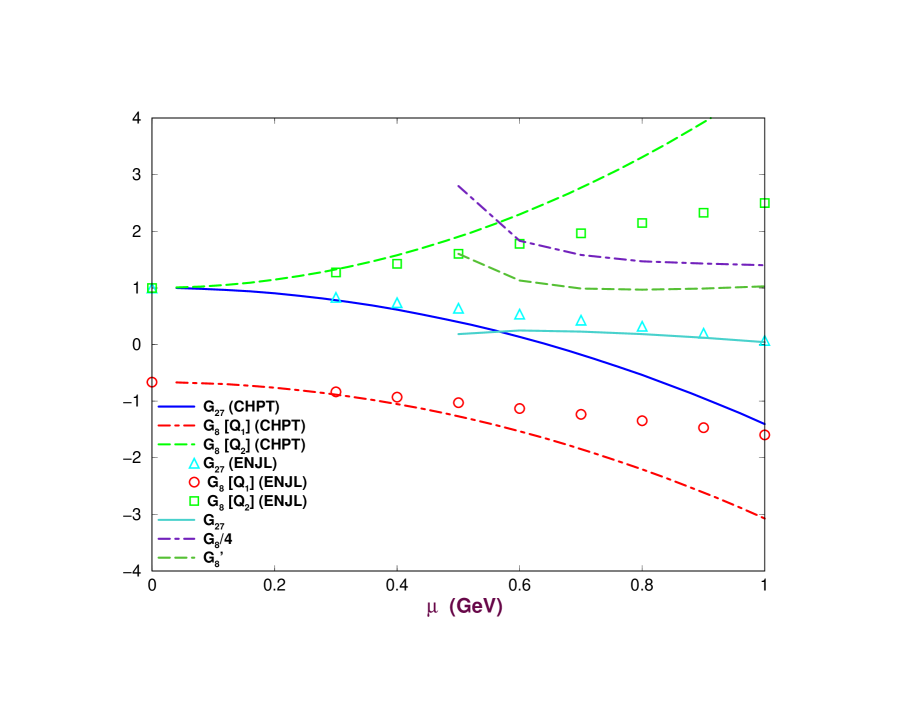
Figure 6: The improvement of the behaviour with $\mu$ of several quantities. Shown are the lowest order result, ENJL result, and when short-distance running is added.

In summary, the results we get for $G_{8}$, $G_{27}$, and $G_{8}^{\prime}$ are

$$4.3< G_{8} <7.5$$

$$0.8< G_{8}^{\prime} <1.1$$

$$0.25< G_{27} <0.40$$ (57)

The bounds have been chosen by looking at both the one-loop and two-loop results in the stability regions in Tables 4 and 5. From (6) we can extract the values

$$-0.75 <b< -0.50$$

$$1.7 <c< 3.7$$ (58)

and we have fixed $a=1$ as explained before. For the $\Delta I=1/2$ rule we get

$$15<\left|\frac{A_{0}}{A_{2}}\right|^{(2)}<40$$ (59)

to order $p^{2}$.

We get a huge enhancement due to the $c$-coupling, it is therefore interesting what do other calculations predict for this coupling. One model where this coupling can be easily extracted is the effective action approach [35]. To order $1/N_{c}$ one gets [35, 36]

$$c = C_{2}(\mu)-1+\Re e\,C_{4}(\mu)+C_{2}(\mu)\,\frac{4\pi\alpha_{s}(\mu)}{N_{c}}\,(2H_{1}+L_{10})(\mu)$$ (60)

$$- 16\frac{B_{0}^{2}(\mu)}{F_{0}^{2}}\,L_{5}(\mu)\left[\Re e\,C_{6}(\mu)+C_{2}(\mu)\,\frac{4\pi\alpha_{s}(\mu)}{N_{c}}\,(2H_{1}+L_{10})(\mu)\right]$$

$$+ O(1/N_{c}^{2})$$

with $\mu=M_{\rho}$, $\alpha_{s}(M_{\rho})=0.70$, $B_{0}(M_{\rho})=1.4$ GeV, and $(2H_{1}+L_{10})(M_{\rho})=-0.015$ [21], we get

$$c = 0.95\pm 0.40\,.$$ (61)

The reason why $c$ is smaller than the present work results is that the long-distance mixing between $Q_{2}$ and $Q_{6}$ is not well treated in this model. In fact this contribution is model dependent already at $O(1/N_{c})$. For instance, it appears in terms of the short-distance value $\alpha_{s}(M_{\rho})$. It is clear that at such scales one has to treat the long distance contributions in a hadronic model and the $\alpha_{s}(M_{\rho})$ above will appear enhanced. Nevertheless, the extra contribution to $c$ coming from the operator $Q_{2}$ [35, 36] both from short-distance origin, namely the term $C_{2}(\mu)-1$, and from long-distance origin, namely the part proportional to $2H_{1}+L_{10}$, give some insight on the potentially large value of $c$.

We cannot easily compare our result with those of [37], their method of calculating the low energy part has no obvious connection to the short-distance evolution and their results cannot be directly compared to ours. The results from the lattice [11] are at rather high values of the quark masses and can thus also not be simply compared to our results.

As stated above, we agree with the calculations of [30] for low values of the scale $\mu$ where we should agree but deviate significantly at higher scales. The earlier Dortmund group results [38] are thus also expected to have significant corrections. The attempts at calculating via more inclusive modes [39] have very large QCD corrections[35, 40]. We see the remnant of this in the large corrections from the $r_{1}$ terms, see Appendix A. The short-distance factors are in fact one of the bigger remaining sources of uncertainty.

7 Results and Conclusions

The main results of this paper are the results for the $O(p^{2})$ couplings $G_{8}$, $G_{27}$, and $G_{8}^{\prime}$ as a function of cut-off $\mu$ for the various operators $Q_{j}$, $j=1,\cdots,6$, as given in Tables 1, 2, and 3. In addition we have corrected our earlier results for $B_{K}(\mu)$ for the routing problem as described in Section 4.1 and presented those in Table 1 as well.

The other main result of this paper is the observation that in the chiral limit the factorizable contribution from $Q_{6}$ is not well defined due to an infrared divergence and we expect that similar problems will show up for the current-current operators when we try to calculate higher order coefficients in the weak chiral perturbation theory Lagrangian. We showed that the total contribution of $Q_{6}$ obtained after adding the non-factorizable and factorizable parts is however well defined. We also expect that he same solution will hold for coefficients of higher order operators in the chiral lagrangian. A corollary of this observation is that the use of $B$-factors in the chiral limit as is common in other treatments of weak non-leptonic operators is not possible in the way they are defined, namely the whole result normalized to the VSA result.

One could use the leading result in $1/N_{c}$ as an appropriate starting point for normalizing the $B_{6}$-parameter in the chiral limit, this is keeping only the $L_{5}$, $L_{8}$, and $H_{2}$ terms but this is difficult to implement for lattice gauge theory calculations. In fact, what in practice people have used [19, 30] for the VSA, i.e. the factorizable part of $Q_{6}$, has been just the large $N_{c}$ part. Of course, this is not in agreement with what is done with other $B$ parameters for current $\times$ current operators like $B_{K}$ where the $1/N_{c}$ factorizable part is always included in the VSA result. After the problems we encountered and the importance of the $B$ parameters to normalize results from different techniques, we believe a new consistent definition of the $B$ parameters should be looked for or just abandon the use of $B$ parameters and quote matrix elements values. We also emphasize that caution should be taken when combining results from different methods for the factorizable and non-factorizable contributions.

When we combine our main results with the Wilson coefficients at one-loop we get nice stable results. Using the Wilson coefficients at two-loops with the inclusion of the $r_{1}$ factors which as we argued in Section 3.2 is necessary we obtain relatively stable values for $G_{8}$ and the coefficient of the weak mass term $G_{8}^{\prime}$ with

$$4.3< G_{8} <7.5$$

$$0.8< G_{8}^{\prime} <1.1$$

$$0.25< G_{27} <0.40$$ (62)

The main uncertainty here is in fact coming from the short-distance coefficients for the octet case and from the long-distance for the 27-plet case. For the $G_{27}$ coupling we obtain a somewhat small value compared to the experimental one. This translates into the following results for the $\Delta I=1/2$ rule in the chiral limit

$$15<\left|\frac{A_{0}}{A_{2}}\right|^{(2)}<40\,.$$ (63)

These results are somewhat large. Nevertheless, we would like to emphasize that we have obtained these results from a next-to-leading in $1/N_{c}$ long-distance calculation and we have passed from the large $N_{c}$ result $|A_{0}/A_{2}|_{N_{c}}=\sqrt{2}$ to values around 20 to 35. One can certainly expect non-negligible $1/N_{c}^{2}$ corrections to our results but the huge enhancement is there. We would also like to stress that we have no free input in our calculation. All parameters have been determined from elsewhere.

From the results above we have also obtained the couplings $b=G_{27}-1$ and $c=(3G_{8}+2G_{27})/5-1$

$$-0.75 <b< -0.50$$

$$1.7 <c< 3.7\,.$$ (64)

Here is then one of our main results, the $\Delta I=1/2$ rule enhancement comes from the Penguin-like topologies $(c)$ in Figure 1, both from $Q_{2}$ which dominates for high values of $\mu$ and from $Q_{6}$ which dominates for small values of $\mu$.

In addition we obtain a value for chiral limit value $\hat{B}_{K}^{\chi}$ as defined in Eq. (69)

$$0.25<\hat{B}_{K}^{\chi}<0.40$$ (65)

and the value for the $\hat{B}_{K}$ parameter in the real case

$$0.59<\hat{B}_{K}<0.79\,.$$ (66)

These two results confirm the ones in [2]. Notice that the different short-distance contribution from $M_{W}$ until the charm quark mass to $G_{27}$ and $\hat{B}_{K}^{\chi}$ has produced

$$\frac{\hat{B}_{K}^{\chi}}{G_{27}}\simeq 1.1\,$$ (67)

instead of $3/4$.

So we have obtained quite good matching for $G_{8}$, $G_{8}^{\prime}$, and $\hat{B}_{K}$ for values of $\mu$ around $0.7-1.04$ GeV and for $G_{27}$ for values of $\mu$ around $0.6-0.8$ GeV. We obtained values for the three parameters of order $p^{2}$ not too far from the experimental ones and a quantitative understanding of the origin of the $\Delta I=1/2$ enhancement. Notice that the values of the cut-off we use to predict our results are not extremely low as in other $1/N_{c}$ approaches, still one would like the matching region to be larger and for somewhat larger values of the cut-off.

Appendix A $\Delta S=1$ and $\Delta S=2$ Wilson Coefficients

In this section we give the numerical values of the Wilson coefficients for the basis of $\Delta S=1$ operators in (16), (17), (3.1), and for the $\Delta S=2$ operator in (20). We give them for the relevant values of the renormalization scale. We have extensively used the formulae in [19].

In all cases we have used $\alpha_{s}(M_{W})=0.121\pm 0.002$, obtained from LEP measurements at the $Z$-peak [5] and then run to two loops to $M_{W}=(80.41\pm 0.10)$ GeV, $\alpha_{s}(m_{b})=0.232\pm 0.003$ obtained from QCD sum rules in the $\Upsilon$ system [41], $\alpha_{s}(M_{\tau})=0.334\pm 0.006$ [42], we then run this value to two-loops up to $\overline{m}_{c}(m_{c})=(1.23\pm 0.05)$ GeV in the $\overline{MS}$ scheme [43] and get $\alpha_{s}(m_{c})=0.42\pm 0.01$. In our approach [19], the penguin operators only get generated from the charm quark mass down since the very small part due to the top quark is not relevant here. We have used the exact solutions of the renormalization group for the running of $\alpha_{s}$ and the quark masses. For $C_{3}$, $C_{4}$, $C_{5}$, and $C_{6}$ we set the small imaginary part due to the top loop to zero. The results to one-loop accuracy are in Table 8 and for two-loops are in Table 9. In the two-loop case we are using the NDR scheme.

If we run the short-distance contribution to two-loops, the matching condition in (27) sets a further coefficient which rends the matrix element scheme independent, i.e.

$$1+\frac{\alpha_{s}(\mu)}{\pi}\,r_{1}\,.$$ (68)

In the case of the $\Delta S=2$ operator, the full two-loop calculation can be found in [32]. In the NDR scheme we have $r_{1}=-7/6$ for the $\Delta S=2$ operator. We obtained it from the right eigenvalues of $\hat{r}_{1}^{T}$ in [19]. So we define

$$\hat{B}_{K}=\left(1+\frac{\alpha_{s}(\mu)}{\pi}\left[r_{1}+\frac{\gamma_{2}}{\beta_{1}}-\frac{\beta_{2}\gamma_{1}}{\beta_{1}^{2}}\right]\right)\,\left[\alpha_{s}(\mu)\right]^{\gamma_{1}/\beta_{1}}B_{K}(\mu)\,.$$ (69)

With $\beta_{1}=-9/2$, $\beta_{2}=-8$, $\gamma_{1}=1$, and $\gamma_{2}=-17/48$. From the discussion in [19] and Section 3.2 it can be seen that this definition is scheme and renormalization scale independent. We have shown in Table 7 this factor in front of $B_{K}(\mu)$ for the case of one-loop running labelled One-loop, two-loop running with $r_{1}=0$, labelled Two-loops, $r_{1}$ at its value, labelled Scheme-Independent (SI), and a version where we use the exact solution of the two-loop running with $r_{1}$ included so as to cancel the full scheme-dependence there too, i.e.

$$\hat{B}_{K}=\left(1+\frac{\beta_{2}}{\beta_{1}}\frac{\alpha_{s}(\mu)}{\pi}\right)^{[\gamma_{2}/\beta_{2}-\gamma_{1}/\beta_{1}+(\beta_{1}/\beta_{2})r_{1}]}\left[\alpha_{s}(\mu)\right]^{\gamma_{1}/\beta_{1}}B_{K}(\mu)\,.$$ (70)

This is labelled exp in Table 7.

$\mu$(GeV)	One-Loop	Two-Loops	SI	exp
0.50	1.04	1.11606	0.46894	0.63252
0.60	1.08	1.14653	0.76287	0.82690
0.70	1.12	1.18208	0.87769	0.91869
0.80	1.15	1.21045	0.94751	0.97817
0.90	1.17	1.23348	0.99680	1.02160
1.00	1.19	1.25267	1.03445	1.05546

Table 7: The coefficients to transform $B_{K}(\mu)$ into $\hat{B}_{K}$. See text for an explanation of the different columns.

The short-distance results for the $\Delta S=1$ Wilson coefficients to two-loops and including the (68) term which can be found in the NDR scheme in [7, 19] for instance, are in Table 10. Here we give the one-loop results in Table 8, two-loop results with $r_{1}=0$ at two-loops in Table 9 and the one with the scheme dependence properly removed, including $r_{1}$, in Table 10. It can be seen that the change from one to two-loops in the NDR scheme is not so large but inclusion of the $r_{1}$ makes a large change.

$\mu$(GeV)	$C_{1}$	$C_{2}$	$C_{3}$	$C_{4}$	$C_{5}$	$C_{6}$
0.50	-0.96466	1.59028	0.01647	-0.03796	0.01116	-0.04663
0.60	-0.84146	1.49560	0.01067	-0.02626	0.00801	-0.03037
0.70	-0.75899	1.43423	0.00710	-0.01839	0.00576	-0.02039
0.80	-0.69875	1.39058	0.00468	-0.01263	0.00403	-0.01356
0.90	-0.65222	1.35759	0.00292	-0.00816	0.00264	-0.00854
1.00	-0.61482	1.33159	0.00158	-0.00455	0.00149	-0.00467

Table 8: Wilson Coefficients of the operators $Q_{1}$ to $Q_{6}$ at one-loop.

$\mu$(GeV)	$C_{1}$	$C_{2}$	$C_{3}$	$C_{4}$	$C_{5}$	$C_{6}$
0.50	-0.80875	1.48719	0.13750	-0.26345	0.01338	-0.27035
0.60	-0.74066	1.43763	0.05198	-0.11330	0.02483	-0.09696
0.70	-0.65083	1.36940	0.03088	-0.07225	0.02160	-0.05673
0.80	-0.58661	1.32243	0.02097	-0.05124	0.01849	-0.03770
0.90	-0.53854	1.28836	0.01516	-0.03796	0.01595	-0.02631
1.00	-0.50087	1.26236	0.01133	-0.02861	0.01388	-0.01860

Table 9: Wilson Coefficients of the operators $Q_{1}$ to $Q_{6}$ at two-loops in the NDR scheme.

$\mu$(GeV)	$C_{1}$	$C_{2}$	$C_{3}$	$C_{4}$	$C_{5}$	$C_{6}$
0.50	-3.73959	4.02465	0.31282	-0.43205	0.03267	-0.33360
0.60	-1.89282	2.35657	0.10089	-0.16996	0.02789	-0.10140
0.70	-1.41708	1.95062	0.05666	-0.10722	0.02258	-0.05469
0.80	-1.17990	1.75588	0.03741	-0.07706	0.01881	-0.03390
0.90	-1.03270	1.63865	0.02665	-0.05877	0.01597	-0.02190
1.00	-0.93034	1.55917	0.01979	-0.04625	0.01374	-0.01397

Table 10: Wilson Coefficients of the operators $Q_{1}$ to $Q_{6}$ at two-loops, the NDR scheme dependence is removed as in discussed in Section 3.2.

References

- [1] E. de Rafael, “Chiral Lagrangians and Kaon CP-Violation”, Lectures given at Theoretical Advanced Study Institute in Elementary Particle Physics (TASI 94), Boulder TASI 1994:0015-86 [hep-ph/9502254]
- [2] J. Bijnens and J. Prades, Nucl. Phys. B444 (1995) 523 [hep-ph/9502363]; Phys. Lett. B342 (1995) 331 [ hep-ph/9409255]
- [3] J.P. Fatelo and J.-M. Gérard, Phys. Lett. B347 (1995) 136
- [4] A. Pich and E. de Rafael, Phys. Lett. B374 (1996) 186 [hep-ph/9511465]
- [5] Review of Particle Physics, C. Caso et al., Eur. Phys. J. C3 (1998) 1
- [6] G. Altarelli and L. Maiani, Phys. Lett. 52B (1974) 351; M.K. Gaillard and B.W. Lee, Phys. Rev. Lett. 33 (1974) 108; A.I. Vainshtein, V.I. Zakharov, and M.A. Shifman, JTEP 45 (1977) 670; F. Gilman and M.B. Wise, Phys. Rev. D20 (1979) 2392; B. Guberina and R. Peccei, Nucl. Phys. B163 (1980) 289
- [7] A. Buras, M. Jamin, M.E. Lautenbacher, and P.H. Weisz, Nucl. Phys. B370 (1992) 69; (Addendum) B375 (1992) 501; Nucl. Phys. B400 (1993) 75 [hep-ph/9211304]; M. Ciuchini, E. Franco, G. Martinelli, and L. Reina, Nucl. Phys. B415 (1994) 403 [hep-ph/9304257]; M. Ciuchini, E. Franco, G. Martinelli, L. Reina, and L. Silvestrini, Z. Phys. C68 (1995) 239.
- [8] A. Buras and J.-M. Gérard, Nucl. Phys. B264 (1986) 371
- [9] W.A. Bardeen, A. Buras, and J.-M. Gérard, Nucl. Phys. B293 (1987) 787; Phys. Lett. 192B (1987) 138.
- [10] J. Kambor, J. Missimer, and D. Wyler, Nucl. Phys. B346 (1990) 17
- [11] L. Lellouch, C.-J. David Lin, UKQCD Coll., preprint CERN-TH-98-307, Talk given at LATTICE 98, Boulder, CO, 13-18 Jul 1998. [hep-lat/9809142]; G. Martinelli, Talk given at LATTICE 98, Boulder, CO, 13-18 Jul 1998, [hep-lat/9810013] and references in these.
- [12] J. Bijnens, E. Pallante, and J. Prades, Nucl. Phys. B521 (1998) 305 [hep-ph/9801326]
- [13] J. Bijnens, Phys. Lett. 152B (1985) 226
- [14] J. Kambor, J. Missimer, and D. Wyler, Phys. Lett. B261 (1991) 496; J. Kambor Nucl. Phys. (Proc. Supp.) B13 (1990) 419; and in Procc. of Workshop on “Effective Field Theories of the Standard Model” Dobogoko (Hungary), (World Scientific , U.-G. Meissner ed.), p. 73 (1992).
- [15] J. Bijnens and J. Prades, Nucl. Phys. B490 (1997) 239 [hep-ph/9610360]
- [16] C. Bernard, T. Draper, A. Soni, H.D. Politzer, and M.B. Wise, Phys. Rev. D32 (1985) 2343
- [17] W.A. Bardeen, J. Bijnens, and J.-M. Gérard, Phys. Rev. Lett. 62 (1989) 1343
- [18] J. Bijnens, Phys. Lett. B306 (1993) 343 [hep-ph/9302217]
- [19] G. Buchalla, A. Buras, and M.E. Lautenbacher, Rev. Mod. Phys. 68 (1996) 1125 [hep-ph/9512380]; A. Buras, “Weak Hamiltonian, CP Violation and Rare Decays”, Technische Univ. Munich preprint TUM-HEP-316/98 [hep-ph/9806471], Lectures given at Les Houches ’97 (F. David and R. Gupta (eds.)).
- [20] J. Bijnens, Phys. Rep. 265 (1996) 369 [hep-ph/9502335] T. Hatsuda and T. Kunihiro, Phys. Rep. 247 (1994) 221 [hep-ph/9401310]
- [21] J. Bijnens, C. Bruno, and E. de Rafael, Nucl. Phys. B390 (1993) 501 [hep-ph/9206236]
- [22] J. Bijnens and J. Prades, Phys. Lett. B320 (1994) 130 [hep-ph/9310355]
- [23] J. Bijnens and J. Prades, Z. Phys. C64 (1994) 475 [hep-ph/9403233]
- [24] J. Bijnens, E. Pallante, and J. Prades, Phys. Rev. Lett. 75 (1995) 1447; (Erratum) 75 (1995) 3781 [hep-ph/9505251]; Nucl. Phys. B474 (1996) 379 [hep-ph/9511388]
- [25] S. Peris, M. Perrottet, and E. de Rafael, J. High Energy Phys. 05 (1998) 011 [hep-ph/9805442]
- [26] M. Knecht, S. Peris, and E. de Rafael, Marseille preprint CPT-98-P-3701 [hep-ph/9809594]
- [27] J. Bijnens, J.-M. Gérard, and G. Klein, Phys. Lett. B257 (1991) 191.
- [28] J. Gasser and H. Leutwyler, Nucl. Phys. B 250 (1985) 465
- [29] R.S. Chivukula, J.M. Flynn, and H. Georgi, Phys. Lett. B171(1986)453
- [30] T. Hambye, G.O. Köhler, E.A. Paschos, P.H. Soldan, and W.A. Bardeen, Phys. Rev. D58 (1998) 014017 [hep-ph/9802300]; T. Hambye, Acta Phys. Polonica B28 (1997) 2479 [hep-ph/9806204]; G.O. Köhler, “A New Analysis of , , and the Rule in the Expansion for Decays”, Dortmund preprint DO-TH 98/11 [hep-ph/9806224]
- [31] E. de Rafael, Nucl. Phys. B (Proc. Suppl.) 7A (1989) 1
- [32] M. Ciuchini, E. Franco, V. Lubicz, G. Martinelli, I. Scimemi, and L. Silvestrini, Nucl. Phys. B 523 (1998) 501; S. Herrlich and U. Nierste, Nucl. Phys. B476 (1996) 27; A.J. Buras, M. Jamin, and P.H. Weisz, Nucl. Phys. B347 (1990) 491
- [33] J. Bijnens, J. Prades, and E. de Rafael, Phys. Lett. B348 (1995) 226 [hep-ph/9411285]
- [34] H. Dosch and S. Narison, Phys. Lett. B417 (1998) 173 [hep-ph/9709215]
- [35] A. Pich and E. de Rafael, Nucl. Phys. B358 (1991) 311
- [36] C. Bruno and J. Prades, Z. Phys. C57 (1993) 585 [hep-ph/9209231]
- [37] S. Bertolini, J.O. Eeg, M. Fabbrichesi, and E.I. Lashin, Nucl. Phys. B514 (1998) 63 [hep-ph/9705244]; V. Antonelli, S. Bertolini, M. Fabbrichesi, and E.I. Lashin, Nucl. Phys. B493 (1997) 281 [hep-ph/9610230]; Nucl. Phys. B469 (1996) 181 [hep-ph/9511341]; V. Antonelli, S. Bertolini, J.O. Eeg, M. Fabbrichesi, and E.I. Lashin, Nucl. Phys. B469 (1996) 143 [hep-ph/9511255]
- [38] J. Heinrich, E.A. Paschos, and J.M. Schwarz, Phys. Lett. B279 (1992)140
- [39] A. Pich and E. de Rafael, Phys. Lett. 189B (1987) 369; A. Pich, B. Guberina, and E. de Rafael, Nucl. Phys. B277 (1986) 197
- [40] A. Pich, in Proc. of the 24th ICHEP, Aug 4-10, 1988 Munich, Germany (Springer-Verlag, R. Kothaus, J.H. Kühn (eds) 1989) ; M. Jamin and A. Pich, Nucl. Phys. B425 (1994) 15 [hep-ph/9402363]
- [41] M. Jamin and A. Pich, Nucl. Phys. B507 (1997) 334; Nucl. Phys. B (Proc. Supp.) 64 (1998) 371; A.H. Hoang Phys. Rev. D57 (1998) 1615; J.H. Kühn, A.A. Penin, and A.A. Pivovarov, Nucl. Phys. B534 (1998) 356.
- [42] R. Barate et al, ALEPH Coll., Eur. J. Phys. C4 (1998) 409.
- [43] S. Narison, Phys. Lett. B341 (1994) 73.