The structure of the Troika: Proton, Photon and Pomeron, as seen at HERA 

Abstract

HERA, the electron-proton collider, enables to probe the proton with a high resolving power due to the deep inelastic scattering reactions at high $Q^{2}$ values. In the low $Q^{2}$ region, one can study the properties of the photon. The large fraction of diffractive events found both in the low and high $Q^{2}$ region allows the study of the Pomeron. A review of what we have learned from HERA so far about the structure of these three objects is presented.

1 Introduction

The ultimate goal of high energy physics is to search for the fundamental constituents of matter and to understand their interactions. This view was already expressed by Newton in the introduction to his book on Optics:

Now the smallest particles of matter cohere by the strongest attraction, and compose bigger particles of weaker virtue; and many of these may cohere and compose bigger particles whose virtue is still weaker, and so on for diverse successions, until the progression ends in the biggest particles on which the operations in chemistry, and the colors of natural bodies depend, and which by cohering compose bodies of a sensible magnitude. There are therefore agents in nature able to make the particles of bodies stick together by very strong attractions. And it is the business of experimental philosophy to find them out.

There are two ways of studying structure of matter: the static way and the dynamic one. In the first approach, symmetry arguments like the ones used by Gel-Mann and Neeman led to the construction of a ‘Mendeleev table’ of the known particles, which eventually brought Gel-Mann and Zweig to postulate the existence of quarks. In the dynamic way one tries to ‘look’ at the particles. This is the ‘Rutherford way’ in which one bombards the target with particles of known identity and searches for structure through the study of the outcome of the bombardment. This was used in the electron–proton deep inelastic scattering (DIS) experiments at SLAC. The underlying assumption was that one uses a projectile whose properties are well known, who behaves like a pointlike structureless particle. Any structure that is being observed following the collision is assigned to the proton and its constituents. This way, the study of the SLAC DIS experiment showed that the DIS cross section behaves like that expected from the interaction of electrons with pointlike particles, called partons, which were later on shown to have the expected properties of quarks, namely spin $\frac{1}{2}$ and fractional charge. This is the quark–parton model (QPM).

1.1 DIS Kinematics

The SLAC DIS experiment introduced the use of some important kinematic variables relevant to the notion of ‘looking’ at the structure of a particle. In figure 1 a lepton with mass $m_{l}$ and four-vector $k(E_{l},\vec{k})$ interacts with a proton with mass $m_{p}$ and four-vector $P(E_{p},\vec{p})$ through the exchange of a gauge vector boson, which can be $\gamma$, $Z^{0}$ or $W^{\pm}$, depending on the circumstances. The four-vector of the exchanged boson is $q(q_{0},\vec{q})$.

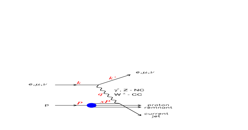
Figure 1: Diagram describing a DIS process on a proton.

With these notations one can define the following variables,

$$q = k-k^{\prime}$$ (1)

$$\nu \equiv \frac{P\cdot q}{m_{p}}$$ (2)

$$y \equiv \frac{P\cdot q}{P\cdot k}$$ (3)

$$W^{2} = (P+q)^{2}$$ (4)

$$s = (k+P)^{2}.$$ (5)

The meaning of the variables $\nu$ and $y$ is most easily realized in the rest frame of the proton. In that frame $\nu$ is the energy of the exchanged boson, and $y$ is the fraction of the incoming lepton energy carried by the exchanged boson. The variable $W^{2}$ is the squared center of mass energy of the gauge–boson proton system, and thus also the squared invariant mass of the hadronic final state. The variable $s$ is the squared center of mass energy of the lepton proton system.

The four momentum transfer squared at the lepton vertex can be approximated as follows (for $m_{l},m_{l}^{\prime}\ll E,E^{\prime}$),

$$q^{2}=(k-k^{\prime})^{2}=m_{l}^{2}+{m_{l}^{\prime}}^{2}-2kk^{\prime}\approx-2EE^{\prime}(1-\cos\theta)<0\ .$$ (6)

The scattering angle $\theta$ of the outgoing lepton is defined with respect to the incoming lepton direction. The variable which is mostly used in DIS is the negative value of the four momentum transfer squared at the lepton vertex,

$$Q^{2}\equiv-q^{2}\ .$$ (7)

One is now ready to define the other variable most frequently used in DIS, namely the dimensionless scaling variable $x$,

$$x\equiv\frac{Q^{2}}{2p\cdot q}\ .$$ (8)

To understand the physical meaning of this variable, one goes to a frame in which masses and transverse momenta can be neglected - the so-called infinite momentum frame. In this frame the variable $x$ is the fraction of the proton momentum carried by the massless parton which absorbs the exchanged boson in the DIS interaction. This variable, defined by Bjorken, is duly referred to as Bjorken-$x$.

The diagram in figure 1 describes both the processes in which the outgoing lepton is the same as the incoming one, which are called neutral current reactions (NC), as well as those in which the nature of the lepton changes (conserving however lepton number) and which are called charged current processes (CC). In the NC DIS reaction, the exchanged boson can be either a virtual photon $\gamma^{*}$, if $Q^{2}$ is not very large and then the reaction is dominantly electromagnetic, or can be a $Z^{0}$ which dominates the reaction at high enough $Q^{2}$ values and the process is dominated by weak forces. In case of the CC DIS reactions, only the weak forces are present and the exchange bosons are the $W^{\pm}$.

1.2 The proton structure function $F_{2}$

The inclusive Born cross section of a NC DIS reaction can be expressed (for $Q^{2}\ll m_{Z}^{2}$) as,

$$\frac{d^{2}\sigma^{Born}}{dxdQ^{2}}=\frac{4\pi\alpha^{2}}{xQ^{4}}\left[\frac{y^{2}}{2}2xF_{1}+(1-y)F_{2}\right],$$ (9)

where $\alpha$ is the electromagnetic coupling constant. The two structure functions $F_{1}$ and $F_{2}$ are related to the transverse and longitudinal $\gamma^{*}p$ cross sections [1].

The relation between the values of $F_{2}$ and their meaning as far as the structure of the proton is concerned can be best seen in a figure adopted from the book of Halzen and Martin [2]. In figure 2 one sees what are the expectations for the distribution of $F_{2}$ as function of $x$ given a certain picture of the proton.

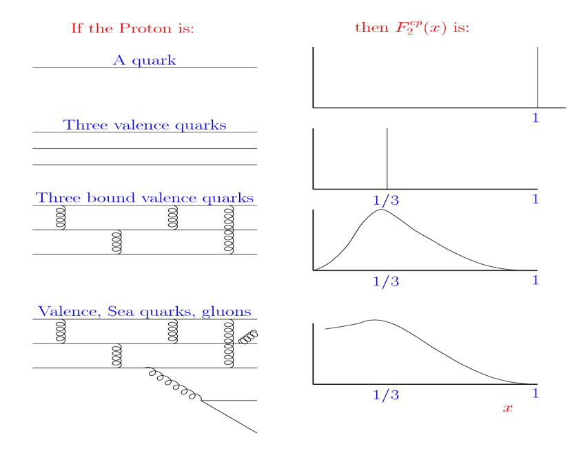
Figure 2: The expected dependence of $F_{2}$ on $x$ given a certain scenario of the structure of the proton.

The static approach mentioned above could explain most properties of the known particles with the proton being composed of three valence quarks. The first measurements of $F_{2}$ [3] indeed confirmed this picture and the QPM was constructed. Later measurements [4] showed that sea quarks and gluons are also present in the proton, as the bottom part of figure 2 shows.

Clearly in order to have a good picture of the structure of the proton one needs to ‘see’ the partons and thus needs the means to have a good resolving power. If we denote by $\Delta$ the sizes one can resolve inside the proton, the higher the virtuality of the exchanged gauge boson in figure 1, the smaller $\Delta$ gets,

$$\Delta\sim\frac{\hbar c}{\sqrt{Q^{2}}}=\frac{0.197\ {\rm GeV\ fm}}{\sqrt{Q^{2}}}.$$ (10)

Thus for $Q^{2}$ = 4 GeV², $\Delta$ = $10^{-14}$cm; for $Q^{2}$ = 400 GeV², $\Delta$ = $10^{-15}$cm; and for $Q^{2}$ = 40000 GeV², $\Delta$ = $10^{-16}$cm.

1.3 The HERA collider

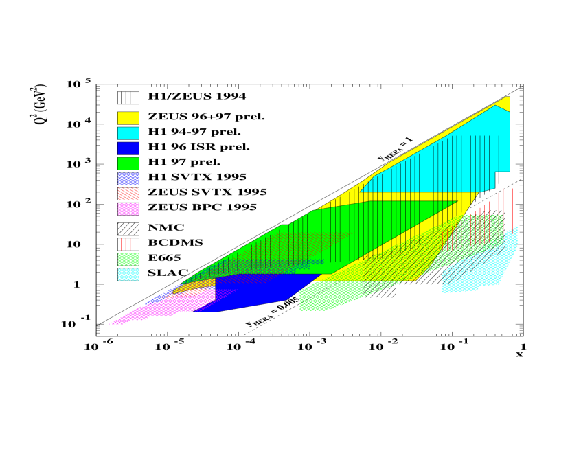
Figure 3: The $x$–$Q^{2}$ kinematic plane of some of the fixed target and of the HERA collider DIS experiments.

How does one achieve high $Q^{2}$ values? One can show that the following relation holds between $Q^{2}$, $x$, $y$ and $s$,

$$Q^{2}\approx xys,$$ (11)

which means that $Q^{2}_{max}\approx s$. Therefore in order to reach large $Q^{2}$ values one needs to build a large $s$ $ep$ collider, which is what was done at DESY with the HERA collider.

HERA [5] is the first $ep$ collider, where a beam of 27.5 GeV electrons (or positrons) collides with a beam of 820 GeV protons yielding a center of mass energy of 300 GeV, or $s\approx$ 90000 GeV².  It has increased the available kinematic $x$–$Q^{2}$ plane by two orders of magnitude going up in $Q^{2}$ and down in $x$. This can be seen in figure 3 which shows the range of existing measurements of some fixed target DIS experiments (SLAC [6], BCDMS [7], E665 [8], NMC [9]) together with the HERA measurements by the H1 [10] and ZEUS [11] collaborations.

During the period 1994–1997 the HERA collider has delivered an integrated luminosity of more than 70 pb^-1 out of which about 47 bp^-1 could be used for physics analyses. At present much effort is concentrated on a luminosity upgrade program, to come into effect in the year 2000, which will deliver an integrated luminosity of about 1 fb^-1 till the year 2005.

1.4 Low-$x$ at HERA

A closer look at figure 3 reveals two facts, one obvious and the other quite surprising. The two HERA collaborations strive to $Q^{2}$ values as high as possible. With the high statistics 1996–1997 data, the experiments have measured some DIS events with $Q^{2}\sim$ 40000 GeV². However, surprisingly, there is an effort also to go to as low $Q^{2}$ as possible, which also allows measuring at very low $x$ values. The reason for trying to reach very low $Q^{2}$ and low $x$ values can be seen from figure 4. In this figure, the dependence of of the proton structure function $F_{2}$ on Bjorken $x$ is shown for three values of $Q^{2}$.

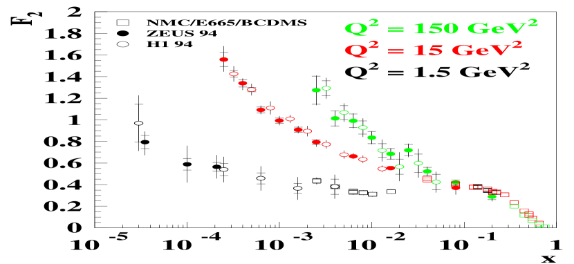
Figure 4: The proton structure function $F_{2}$ as function of $x$ for three $Q^{2}$ values.

One sees a clear rise of the structure function with decreasing $x$. However, as $Q^{2}$ gets smaller this rise is less steep. What does this plot tell us? In order to understand it, let us first look at the variable $x$. It is related to $Q^{2}$ and to $W$ (the $\gamma^{*}p$ center of mass energy) as,

$$W^{2}=Q^{2}(\frac{1}{x}-1)+m_{p}^{2}\approx\frac{Q^{2}}{x},$$ (12)

where the approximate relation is good for low $x$ values. Thus for fixed $Q^{2}$, going in the low $x$ directions means increasing $W$.

The proton structure function $F_{2}$ can be related to the total $\gamma^{*}p$ cross section $\sigma_{tot}^{\gamma^{*}p}$ through the relation,

$$F_{2}=\frac{Q^{2}(1-x)}{4\pi^{2}\alpha}\frac{Q^{2}}{Q^{2}+4m_{p}^{2}x^{2}}\sigma_{tot}^{\gamma^{*}p}\approx\frac{Q^{2}}{4\pi^{2}\alpha}\sigma_{tot}^{\gamma^{*}p},$$ (13)

where we have used the Hand [12] definition of the flux of virtual photons, and again the approximate expression holds for low $x$ values. Thus, the behaviour seen in figure 4 can be interpreted as a rising $\gamma^{*}p$ cross section with increasing $W$, where the increase gets steeper as $Q^{2}$ increases. How does this steepness decrease as one goes to lower and lower values of $Q^{2}$? Is there a sharp or a smooth transition? What happens at $Q^{2}$ = 0 when the photon is real?

1.5 Low $Q^{2}$ at HERA

These questions motivated the HERA experimentalists to try to measure the behaviour of the structure function at low $Q^{2}$ and also to measure the real photoproduction cross section in the high $W$ region of HERA. How does one do low $Q^{2}$ physics in a machine which was built to reach highest possible $Q^{2}$ values? A look at equation (6) shows that the value of $Q^{2}$ is determined by the energies of the incoming ($E$) and the outgoing ($E^{\prime}$) electrons and by the scattering angle $\theta$ of the outgoing electron with respect to the incoming one,

$$Q^{2}=2EE^{\prime}(1-\cos\theta).$$ (14)

To get to low values of $Q^{2}$, the angle $\theta$ has to be small and therefore the scattered electron remains in the beam pipe. However, if one can arrange to measure the outgoing electron at very low scattering angles in a special detector, one has a handle of measuring low $Q^{2}$ photons, with the possibility to go down to the quasi–real photon case for extremely small angles.

The two experiments, H1 and ZEUS, have each built a small calorimeter at a distance of about 30 m from the interaction point which allows to detect electrons which were scattered by less than 5 mrad with respect to the incoming electron direction. This ensures that the virtuality of the exchanged photons is in the range $10^{-8}<Q^{2}<0.02$ GeV², with the median $Q^{2}\approx 10^{-5}$ GeV². A diagrammatic example of an event produced by a quasi–real photon, denoted as a photoproduction event, is shown in figure 5.

Figure 5: A diagrammatic example of a photoproduction event in the ZEUS detector, where the scattered electron is detected in the small angle electron calorimeter LUMI.

In this event the scattered electron is detected in the electron calorimeter. This calorimeter is part of the luminosity detector, which includes also a photon detector at a distance of about 100 m from the interaction point.

The way to tag events with $Q^{2}$ in the range of 0.1-1 GeV² is through two methods. One methods is based on moving the position of the interaction vertex towards the incoming electron beam. By shifting the vertex in this direction one increases the possibility to measure low-angle scattered electrons in the rear part of the main calorimeter. The other method is similar to that in the photoproduction case described above. It consists of building a special calorimeter to detect the small-angle scattered electron. This was done by building two parts of a small calorimeter around the beam pipe which accordingly was named the beam-pipe calorimeter (BPC). Both methods are diagrammatically described in figure 6.

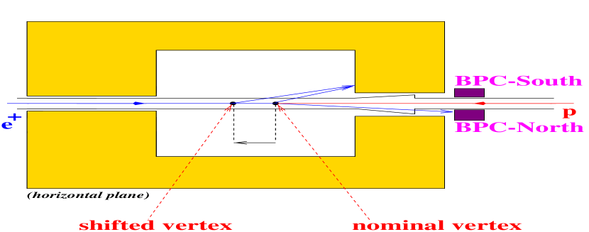
Figure 6: A diagrammatic description of the ZEUS detector showing the beam–pipe calorimeter (BPC), and the nominal and the shifted vertex positions.

It is thus clear from the above discussion that HERA has also become a source of high $W$ quasi-real photons. In fact, the highest $W$ photon beams before HERA were in the range of 20 GeV and HERA has increased this by one order of magnitude. This allows among other things to study the structure of the photon at low $x$ values.

1.6 The concept of the structure of the photon

What do we mean by ‘the structure of the photon’? The photon is the gauge particle mediating the electromagnetic interactions and thus one would expect it to be an elementary point-like particle. How can one talk then about the structure of the photon? We know from low $W$ data that when the photon interacts with hadrons it behaves like a hadron. This property is well described by the vector dominance model (VDM) [13] in which the photon turns first into a hadronic system with the quantum numbers of a vector meson before it interacts with the target hadron. The justification of this picture was given by Ioffe [14] who used time arguments. Just like a photon can fluctuate in QED into a virtual $e^{+}e^{-}$ pair (figure 7a) it can also fluctuate into a $q\bar{q}$ pair (figure 7b).

Figure 7: Fluctuation of a photon into (a) an $e^{+}e^{-}$ pair, (b) a $q\bar{q}$ pair.

As long as the fluctuation time $t_{f}$ is small compared to the interaction time $t_{int}$ the photon will interact directly with the hadron. However if $t_{f}\gg t_{int}$ the interaction will be between the $q\bar{q}$ pair and the hadron and will look like a hadronic interaction. The fluctuation time of a photon with energy $E_{\gamma}$ which is large compared to the hadronic mass $m_{q\bar{q}}$ into which the photon fluctuates ($E_{\gamma}\gg m_{q\bar{q}}$) is given by,

$$t_{f}\simeq\frac{2E_{\gamma}}{m^{2}_{q\bar{q}}}.$$ (15)

This is the case for a real photon. For a virtual photon $\gamma^{*}$ the fluctuation time is given by,

$$t_{f}\simeq\frac{2E_{\gamma}}{m^{2}_{q\bar{q}}+Q^{2}}.$$ (16)

The interaction time with a proton is of the order of its radius, $t_{int}\approx r_{p}\sim$ 1 fm. Thus while a high energy real photon develops a structure due to its long fluctuation time compared to the interaction time, a highly virtual photon has no time to acquire a structure before probing the proton.

The structure of real photons has been indeed studied in $e^{+}e^{-}$ interactions where the photon structure function $F_{2}^{\gamma}$ has been measured in a similar DIS type of experiment as on the proton. A diagram describing this is shown in figure 8 where the proton target is replaced by a quasi-real photon target at the vertex where the electron has a very small scattering angle.

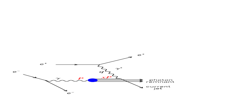
Figure 8: Diagram describing a DIS process on a quasi-real photon using the reaction $e^{+}e^{-}\to e^{+}e^{-}X$.

The $x$ values reached in these experiments were not small due to the fact that the available $W$ of the $\gamma^{*}\gamma$ system was relatively small.

As stated above, also at HERA one can study the photon structure. The exchanged photon, which at high $Q^{2}$ is a probe, can change its role at very low $Q^{2}$ and become a quasi-real photon target. It can be probed by a high transverse momentum parton from the proton. We shall discuss this in more details in section 3.

The high $W$ values attained at HERA give a large lever arm to study the energy behaviour of the total photoproduction cross section $\sigma_{tot}({\gamma p})$. Does it show the same behaviour as the total hadron-hadron cross sections? The latter were shown by Donnachie and Landshoff [15] to have a simple behaviour, independent on the incoming hadron, and well described by the Regge model.

Donnachie and Landshoff (DL) succeeded to describe all available $\bar{p}p$, $pp$, $K^{\pm}p$, and $\pi^{\pm}p$ total cross section values by a simple parameterization of the form $\sigma_{tot}=Xs^{0.0808}+Ys^{-0.4525}$, where $s$ in the square of the total center of mass energy and $X$ and $Y$ are parameters depending on the interacting particles. The value of $X$ is constrained to be the same for particle and anti-particle beams to comply with the Pomeranchuk theorem [16]. The power of the first term is connected in the Regge picture to the intercept of the exchanged Pomeron at $t$ = 0, ($\alpha_{IP}(0)$ = 1.08), while the second term comes from the intercept of the Reggeon ($\alpha_{IR}(0)$ = 0.5475). The total cross section data of $\bar{p}p,pp$ and $\pi^{\pm}p$ are shown in figure 9 together with the DL parameterization.

Figure 9: The total cross section data of $\bar{p}p,pp$ and $\pi^{\pm}p$ as function of the center of mass energy $\sqrt{s}$. The DL parameterization is shown as the solid lines.

One of the first measurements at HERA was that of the total $\gamma p$ cross section $\sigma_{tot}({\gamma p})$.

Figure 10:

The total photoproduction cross section data measured by H1 and ZEUS together with the fixed target data as function of $W$. The full line and the dotted line are the DL parameterization prediction for $\alpha_{IP}$=1.08 and 1.1, respectively. The dashed line is that of the ALLM [19] parameterization.

The measurement showed that the hadronic behaviour of the photon, observed at lower energies, holds also in the HERA $W$ range. The measurements of H1 [17] and ZEUS [18], shown in figure 10, agree well with the expectations of the DL parameterization for photoproduction.

1.7 Diffraction in photoproduction and DIS - the Pomeron

If the photon behaves like a hadron, one expects to see diffractive processes at HERA energies. Indeed it turns out that about 40 % of the photoproduction events are due to diffractive processes. The diffractive reactions are described by diagrams in which the exchange carries the quantum number of the vacuum, is a colorless object and is referred to in the Regge language as the Pomeron trajectory. The existence of such a trajectory was first suggested by Gribov [23] in order to avoid contradictions with unitarity in the crossed channel. The trajectory was named after Pomeranchuk by Gel-Mann. In a reaction in which a Pomeron [24] is exchanged the proton remains intact or is being diffractively dissociated into a state with similar quantum numbers (Gribov-Morrison rule [25]). Thus there is a large rapidity gap between the proton or its dissociated system and the hadrons belonging to the system into which the photon diffracted. These large rapidity gap events were observed in the photoproduction sample at HERA.

Figure 11:

Diagram of a diffractive DIS event in which a photon of virtuality $Q^{2}$ diffracts into a system $X$ at a $\gamma^{*}p$ center of mass energy $W$ and where the four momentum transfer squared at the proton vertex is $t$.

One of the big surprises at HERA were the observation of large rapidity gap events also in the DIS events [20, 21]. The existence of such events meant that also a virtual photon can diffract. This indicated that a process of DIS which is believed to be a hard process because of the presence of a large scale, $Q^{2}$, can also possess properties like diffraction which are expected in a soft, low scale reactions. This interplay [22] of soft and hard processes will be discussed later. The observation of diffractive processes in the DIS sample opened up the possibility of studying the structure of the Pomeron in a DIS type experiment as depicted in figure 11.

Let us finish this section by figure 12 which

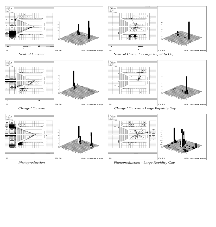
Figure 12: Some events as seen in the ZEUS detector at HERA (see text).

shows events resulting from electron–proton interactions, as seen in the ZEUS detector (left part of each picture). The initial electron and proton are in the beam pipe and not seen in the detector. The electron enters the detector from the left and the proton from the right. The right part of each picture shows a lego plot of the transverse energy flow as function of the spatial angle.

The three events depicted on the left side of the page are three different processes: NC DIS (top) in which the scattered electron performs an almost U–turn and one of the partons of the proton emerges as a jet; CC DIS (center), where the initial electron turns into a neutrino which is undetected and one of the hit partons from the proton emerges as a jet, thus producing an unbalance in the transverse energy; photoproduction reaction (bottom), a process where the scattered electron emerges at a very small angle and thus remains undetected in the beam pipe and the quasi–real photon interacts with one of the partons of the proton producing two high transverse momentum jets. The three events on the right hand side of the page are similar processes, respectively, with the distinction that the proton remains intact also after the interaction, producing a large rapidity gap in the forward part of the detector, indicating that the reaction is diffractive in nature and pointing to the presence of the Pomeron.

1.8 The ‘Fathers’

We have so far introduced the concept of the structures of the proton, the photon and the Pomeron, all of which can be studied at HERA, and details of which will be described in the next sections. We will conclude this lengthy introductory section with the pictures of the ‘fathers’ of these three objects: Rutherford (proton), Einstein (photon) and Gribov (Pomeron). Also shown is a picture of Pomeranchuk who gave his name to the Pomeron and made remarkable contributions to the theory of hadron-hadron interactions.

Figure 13: Rutherford

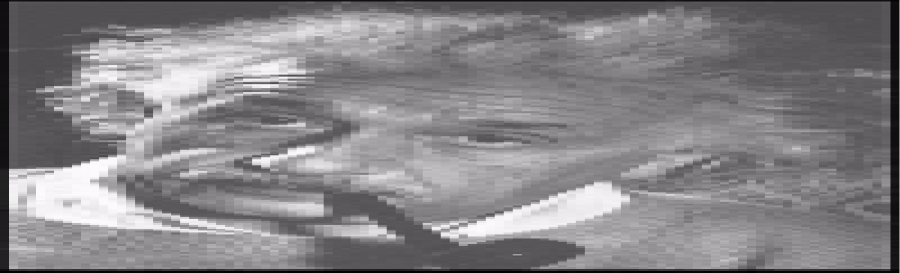
Figure 14: Einstein

Figure 15: Gribov

Figure 16: Pomeranchuk

2 The structure of the proton

As mentioned in the introduction, HERA was built foremost to look deeper inside the proton by providing very high $Q^{2}$ DIS interactions [26]. How will we know that we see something new? One way would be for instance to discover a lepto-quark, which is a particle which - if it exists - may be seen at HERA as an s-channel resonance in the $e$-$q$ system. Experimentally, such a particle would show up as a peak in the $x$ distribution, where the position of the peak is related to the lepto-quark mass $m_{LQ}$ as,

$$m^{2}_{LQ}=xs.$$ (17)

The present lower limits of a lepto-quark from the Tevatron are larger than 200 GeV, which means that for the available $s$ at HERA, a peak would appear at high $x>$ 0.5. A look at figure 3 shows that in order to reach such high values of $x$ one needs very large $Q^{2}$ interactions. With the present luminosities the data statistic are insufficient for a clear observation.

2.1 NC and CC cross sections

Another way to search for new physics is to look for deviations from the Standard Model predictions of values like the NC and CC cross sections at high $Q^{2}$. Such a comparison was done with the data from 1993–1995, which can be seen in figure 17.

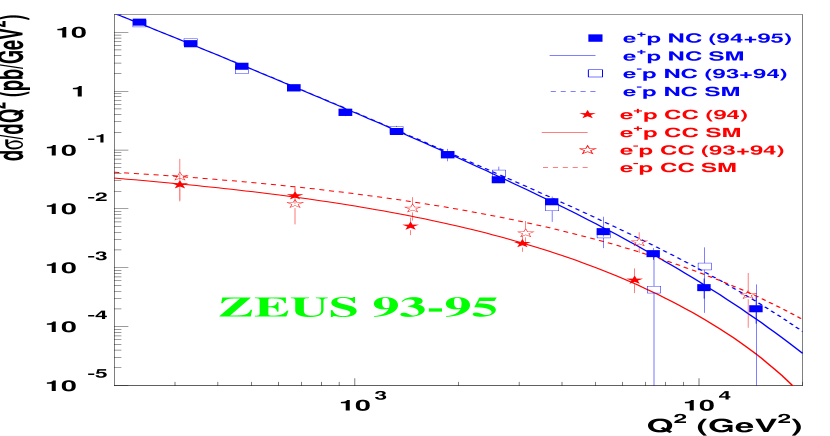
Figure 17: The cross section of NC and CC events as function of $Q^{2}$ for $e^{+}p$ and $e^{-}p$ interactions. The solid and dashed lines are predictions of the Standard model for $e^{+}p$ and $e^{-}p$ interactions, respectively.

This figure is very educative, a ‘textbook’ type of figure, and thus deserves a detailed discussion. In the NC case one has for the low $Q^{2}$ region the dominance of the electromagnetic interaction mediated by the photon which predicts a behaviour like

$$\frac{d\sigma}{dQ^{2}}\sim\frac{1}{Q^{4}}.$$ (18)

At high $Q^{2}$, the weak force mediated in the NC case by the $Z$ boson is important and contributes,

$$\frac{d\sigma}{dQ^{2}}\sim\frac{1}{Q^{4}}\left(\frac{Q^{2}}{Q^{2}+m_{Z}^{2}}\right)^{2}.$$ (19)

In case of the CC interactions only the weak force mediated by the $W$ boson contributes,

$$\frac{d\sigma}{dQ^{2}}\sim\frac{1}{Q^{4}}\left(\frac{Q^{2}}{Q^{2}+m_{W}^{2}}\right)^{2}.$$ (20)

Thus at low $Q^{2}$, ($Q^{2}\ll m_{Z}^{2}$) one expects $\frac{d\sigma}{dQ^{2}}$(NC) $\gg\frac{d\sigma}{dQ^{2}}$(CC). In the region $Q^{2}\sim m_{Z}^{2}$ one expects the two cross sections to be of the same order, $\frac{d\sigma}{dQ^{2}}$(NC) $\sim\frac{d\sigma}{dQ^{2}}$(CC). These predictions of the Standard Model are nicely borne out by the data shown in figure 17. A closer look into the exact formulae [1] shows that the cross sections are higher for the $e^{-}p$ interactions than for the $e^{+}p$ ones, again in agreement with the data.

2.2 $W$ mass determination

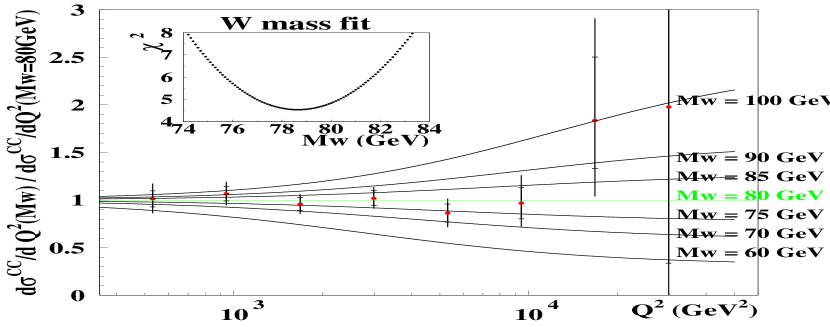
Figure 18: The ratio of the CC differential cross section at a value of $m_{W}$ given at the left of the figure, to that at $m_{W}$ = 80 GeV, as function of $Q^{2}$. The insert gives the $\chi^{2}$ as function of $m_{W}$.

Another nice result comes from the CC events. It is clear from equation (20) that the cross section depends on the $W$ mass and thus by fitting the CC differential cross section one can in principle determine $m_{W}$. A preliminary attempt of such a determination is shown in figure 18 which results in [27]

$$m_{W}=78.6^{+2.5}_{-2.4}({\rm stat})^{+3.3}_{-3.0}({\rm syst})\ {\rm GeV}.$$ (21)

This value is in good agreement with the world average one [28]. Clearly the large error on the mass will be reduced once the high luminosity run will increase the statistics of the data in this high $Q^{2}$ region.

2.3 Signs for new physics?

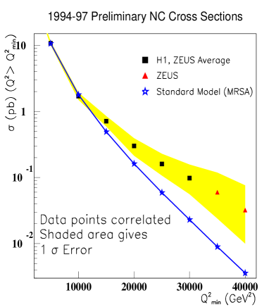
Figure 19: The cross section of NC and CC events as function of $Q^{2}$ for $e^{+}p$ and $e^{-}p$ interactions. The solid and dashed lines are predictions of the Standard model for $e^{+}p$ and $e^{-}p$ interactions, respectively.

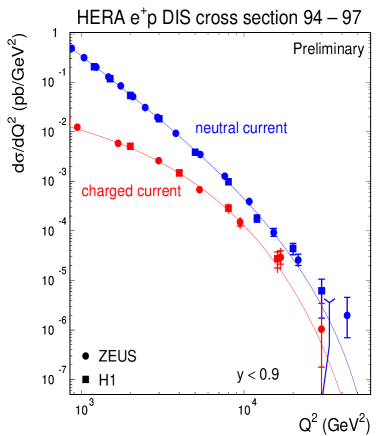
Figure 20: The differential cross section $\frac{d\sigma}{dQ^{2}}$ of NC and CC events from the 1994–1997 data as function of $Q^{2}$ for $e^{+}p$ interactions as measured by the H1 and ZEUS collaborations.. The solid lines are predictions of the Standard model.

All the above was true for the 1993–1995 data. About a year ago, after adding the 1996 data, there was a big excitement due to a possible sign of deviation from the predictions of the Standard Model. Both the H1 [29] and ZEUS [30] collaborations observed an excess of events at very high $Q^{2}$. Preliminary results shown at the Lepton–Photon Symposium in 1997 [31] indicated a deviation from the Standard Model predictions which seemed to increase with $Q^{2}$, as can be seen in figure 20 [32]. The figure shows the NC cross section of the events with $Q^{2}$ above a minimum value of $Q^{2}_{min}$ which is in excess of the expectations of the Standard Model. The shaded area gives the 1 standard deviation error of the data.

In the meantime both collaborations finished to analyze their 1997 data and published preliminary results of $\frac{d\sigma}{dQ^{2}}$ of the NC and CC data accumulated during 1994–1997 [33, 34, 27], displayed in figure 20. The following observations can be made:

• There is good agreement between the data of the H1 and ZEUS collaborations.

• The cross section for NC and CC events are of the same order for $Q^{2}\geq m^{2}_{W,Z}$.

• In the region of $Q^{2}\geq 10^{4}$ GeV² the cross section measurements are still statistics limited.

• Both NC and CC cross sections seem to show some excess over the Standard Model predictions at the highest measured $Q^{2}$ point.

We will have to wait for much higher statistics in order to evaluate the significance of the excess at high $Q^{2}$.

It is clear that in order to make any claim of a disagreement with the Standard Model, one first has to be able to state how well the predictions are known. This was estimated [29, 30] to be 6.5 %, where the main uncertainty comes from the knowledge of the parton distributions in the proton. This can also be seen in the left-hand side of figure 21 where the NC differential cross section of the 94–97 data are shown together with the predictions of the Standard Model. The right-hand side shows the ratio of the data to the prediction, where in the prediction a particular representation (CTEQ4D [35]) of parton distribution parameterizations has been used. The band, labeled as PDF band, shows the uncertainty of the prediction due to the uncertainty in the parton distributions.

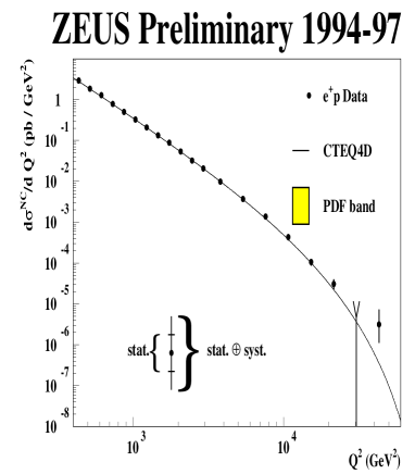
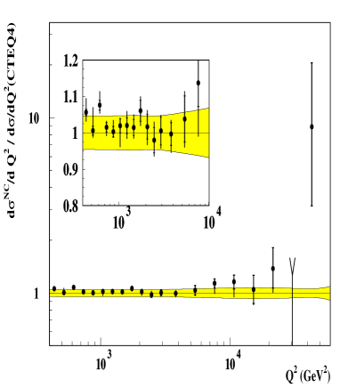
Figure 21: Left part: $d\sigma/dQ^{2}$ of the 94–97 NC data. The line is the predictions of the Standard Model. Right part: the ratio of the data to the prediction using for the latter the CTEQ4D parameterization of the parton distribution function (PDF). The band, shows the uncertainty of the ratio due to the uncertainty in the parton distributions.

2.4 Parton distributions

Why should there be an uncertainty in the parton distributions? Is not QCD a theory which describes the interactions of quarks and gluons? As we all know, the answer to this rhetoric question is connected to the behaviour of the strong coupling $\alpha_{S}(Q^{2})$ which becomes too large at low $Q^{2}$ to enable a reliable calculation. Only when the scale $Q^{2}$ is large enough one can do a perturbative QCD (pQCD) calculation. This fact does not allow to calculate the parton distribution functions from first principles. We can nevertheless predict the parton distribution at a larger scale once we know them at a lower scale, due to the QCD factorization theorem [36]. This theorem allows to factorize the cross section into short distance phenomena, fully calculable in pQCD due to the presence of a large scale, and long distance phenomena which include the flux of universal incoming partons. The latter cannot be calculated perturbatively and has to be taken from experimental data. The Dokshitzer-Gribov-Lipatov-Altarelli-Parisi (DGLAP) [37] equations enable the evolution of the parton distribution to any $Q^{2}$ once they are given at a starting value $Q^{2}_{0}$. How low can one go with the value of the starting scale $Q^{2}_{0}$? Will will try to answer this somewhat later. Before doing that, it is educative to point out what are the assumptions used in the DGLAP evolution equations.

Figure 22: Left part: A diagram describing the development of a parton chain in an $ep$ interaction. Each parton has a value of $x_{i}$ and of transverse momentum $k_{i}$. Also given are the assumptions about these values for the DGLAP and the BFKL evolution equation. Right part: the path taken in the $x,Q^{2}$ plane when evolving through the DGLAP and the BFKL equations.

The DGLAP evolution equations allow us to go from a given point ($x_{0},Q_{0}^{2}$) to another point ($x_{1},Q_{1}^{2}$) so that $x_{1}<x_{0}$ and $Q^{2}_{1}>Q^{2}_{0}$. During this evolution there is strong ordering in the transverse momentum of the parton chain and also ordering in their $x$ values (see figure 22). Another evolution equation has been suggested by Balitzki-Fadin-Kuraev-Lipatov (BFKL) [38] which deals with cases in which there is only evolution in $x$. There is no ordering in the transverse momentum of the partons but only strong ordering in their $x$ values (figure 22). We will not discuss it further in this talk.

2.5 Scaling violation

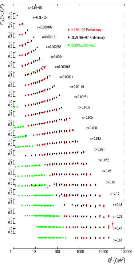
Figure 23: The dependence of the proton structure function $F_{2}$ on $Q^{2}$ for fixed values of $x$.

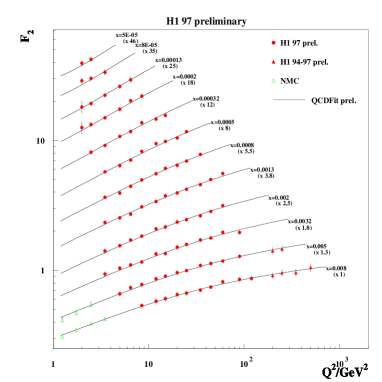
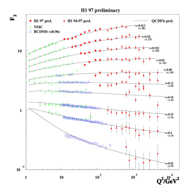
Figure 24: Comparison of the scaling violation behaviour of $F_{2}$ with the results of a next-to-leading order (NLO) DGLAP evolution equation.

Back to the data. In figure 24 one sees the dependence of the proton structure function $F_{2}$ on $Q^{2}$ for fixed values of $x$ [39]. The data come from the two HERA experiments and from some of the lower energy fixed target experiments. One sees a remarkable agreement between the data of different experiments. One can also see the positive scaling violation at low $x$ and the approximate scaling at intermediate $x$. This can be seen in more details, together with the negative scaling violation at high $x$, in figure 24. In this figure one also sees that a next-to-leading-order (NLO) QCD fit using the DGLAP equations can describe the data up to quite high $Q^{2}$ values.

2.6 Global QCD fits

How does one do a QCD fit to the data and gets out of it parton distributions? One assumes a mathematical form in the $x$ variable for the different parton distributions at a given $Q^{2}_{0}$. One uses the DGLAP equations to evolve the parton distributions to any other $Q^{2}$ value where measurable quantities exist. By fitting the calculations to the data, the parameters of the initial parton distributions which give the best fit are thus determined. Measurable quantities do not necessarily have to be only structure functions. Drell-Yan cross sections, W assymetries, direct photon production yields, inclusive jet cross sections - all such quantities are included in a global fit. As an example we show in table 1 a list of such variables and the number of data points used in a recent global QCD fit by Martin-Roberts-Stirling-Thorne (MRST) [40]. They use in total close to 1500 data points and obtain fits with $\chi^{2}$ of the order of $\sim$ 1-1.2 per degree of freedom.

Process	Experiment	Measurable	Data Points
DIS	BCDMS	$F_{2\ H}^{\mu},F_{2\ D}^{\mu}$	324
	NMC	$F_{2\ H}^{\mu},F_{2\ D}^{\mu},F_{2\ n/p}^{\mu}$	297
	SLAC	$F_{2\ H}^{e}$	70
	E665	$F_{2\ H}^{\mu},F_{2\ D}^{\mu}$	70
	H1	$F_{2\ H}^{e}$	172
	ZEUS	$F_{2\ H}^{e}$	179
	CCFR	$F_{2\ Fe}^{\nu},x\ F_{3\ Fe}^{\nu}$	126
Drell-Yan	E605	$sd\sigma/d\sqrt{\tau}dy$	119
	E772	$sd\sigma/d\sqrt{\tau}dy$	219
	NA-51	$A_{DY}$	1
	E886	$pd/pp$	11
W-prod.	CDF	Lepton asym.	9
Direct $\gamma$	WA70	$Ed^{3}\sigma/d^{3}p$	8
	UA6	$Ed^{3}\sigma/d^{3}p$	16
	E706	$Ed^{3}\sigma/d^{3}p$	19
Incl. Jet	CDF	$d\sigma/dE_{t}$	36
	D0	$d\sigma/dE_{t}$	26

Table 1: A list of measurables used in a global QCD fit to determine parton distribution functions.

The resulting parton distributions of the MRST global QCD fit at a scale of $Q^{2}$ = 20 GeV² are shown in figure 25.

Figure 25: Parton density distributions as function of $x$ of the MRST global QCD fit at a scale of $Q^{2}$ = 20 GeV².

At large $x$ only the valence, $u$ and $d$, quarks contribute appreciably. The sea quark densities rise sharply as $x$ decreases. However the rise of the gluon density is much sharper and in order to fit into the same figure with all the quarks it had to be suppressed by an order of magnitude. The physical meaning of the parton density functions is the number of partons per unit of rapidity. Thus according to the MRST parameterization there are more than 20 gluons per unit of rapidity at $x$ = $10^{-4}$ at a scale of $Q^{2}$ = 20 GeV². It is also interesting to see how the proton momentum is distributed among the partons according to the MRST parameterization at different $Q^{2}$ values. This can be seen in table 2 from which one learns that the gluon carries close to 40 % of the proton momentum and this fraction increases with $Q^{2}$, while the momentum fraction carried by the valence quarks decreases with $Q^{2}$.

$Q^{2}$(GeV2)	$u_{v}$	$d_{v}$	$2\bar{u}$	$2\bar{d}$	$2\bar{s}$	$2\bar{c}$	$2\bar{b}$	g
2	0.310	0.129	0.058	0.075	0.037	0.001	0.000	0.388
20	0.249	0.103	0.063	0.077	0.046	0.017	0.000	0.439
20000	0.178	0.074	0.070	0.080	0.058	0.036	0.026	0.472

Table 2: The momentum distribution among partons according to the MRST parameterization.

2.7 Behaviour of $F_{2}$ at low $x$

Back to the $F_{2}$ behaviour. The good agreement with the QCD evolution calculations can also be seen in figure 26 where this time the $F_{2}$ data are shown as function of $x$ for fixed $Q^{2}$ values.

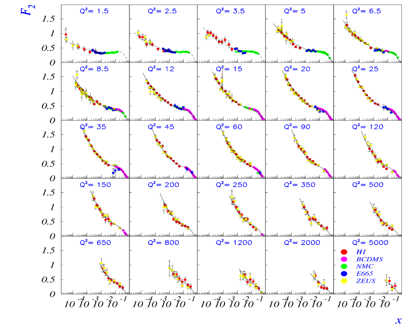
Figure 26: $F_{2}$ as function of $x$ for fixed $Q^{2}$ values (in GeV²) as indicated in the figure, for the HERA 94 data together with some fixed target data. The curves are the result of a NLO QCD fit.

We see again the good agreement between the HERA and the fixed target data. Another interesting observation from this figure is the fact that the NLO DGLAP equations seem to give a good description of the data down to $Q^{2}$ values as low as 1.5 GeV². However most striking is the strong rise of $F_{2}$ with decreasing $x$ in all $Q^{2}$ bins. The steepness of this rise seems to be $Q^{2}$ depended; it gets shallower as $Q^{2}$ decreases. This behaviour seems to be embedded in the QCD evolution equations.

Let us try to quantify the rise using a phenomenological argument. In order to do so it is easier to return to equation (13) which relates $F_{2}$ to the $\gamma^{*}p$ total cross section and which, for low $x$, reads

$$F_{2}\approx\frac{Q^{2}}{4\pi^{2}\alpha}\sigma_{tot}^{\gamma^{*}p}.$$ (22)

Regge theory, which gives a good description of the behaviour of the total cross section with energy, expects

$$\sigma_{tot}\sim s^{\alpha(0)-1},$$ (23)

where $s$ is the squared center of mass energy and $\alpha(0)$ is the intercept of the leading trajectory. Since in the $\gamma^{*}p$ case the squared center of mass energy is $W^{2}$ and since for low $x$ we have $W^{2}\approx Q^{2}/x$, one would expect that for fixed $Q^{2}$

$$F_{2}\sim x^{-\lambda},$$ (24)

where $\lambda=\alpha(0)-1$. One thus restricts the data to the low $x$ region, say $x<$ 0.1, and for each $Q^{2}$ region fits equation (24) to the data and obtains $\lambda(Q^{2})$. From the introductory section where we mentioned the total photoproduction cross section behaviour we know that $\lambda(Q^{2}=0)$ = 0.08. What happens at higher $Q^{2}$? This we can see in figure 27 which shows the result of such a fit done by the H1 collaboration [41].

Figure 27: The behaviour with $Q^{2}$ of the exponent $\lambda$ from fits of the form $F_{2}\sim x^{-\lambda}$ at fixed $Q^{2}$ values and $x<$0.1.

In spite of the large error bars, one sees the trend of increasing $\lambda$ from a value of about 0.15 at low $Q^{2}$ to about 0.3 at intermediate $Q^{2}$. The precision of the data does not allow any conclusion about the continuation of the rise at higher $Q^{2}$. Since in the limit of $Q^{2}$ = 0 the value should decrease to 0.08, it is of interest to see what is happening between 0.15 and 0.08. Is the transition sharp or smooth?

2.8 The low $Q^{2}$ region

What is so interesting about the transition? The total photoproduction cross section shows the same behaviour as the total hadron-hadron cross sections. They are both dominated by low transverse momentum interactions, ‘soft’ interactions, and can be described in the Regge language by the exchange of a DL type Pomeron trajectory. The DIS domain is well described by QCD, the physics of which is believed to be dominated by ‘hard’ interactions. Clearly not all of the ‘soft’ region is only soft just as not all of the ‘hard’ regime is completely hard. There is an interplay between soft and hard interactions (see [22]). We would like to find where this transition occurs and maybe learn more about the properties of these two domains. This is what drove the two HERA experiments to measure also in the very low $Q^{2}$ region by methods described in the introductory section.

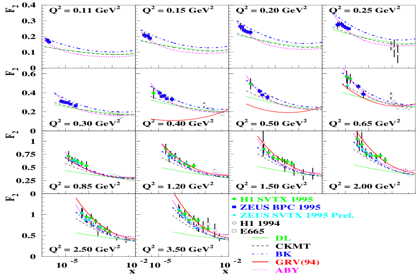
Figure 28: $F_{2}$ as function of $x$ for fixed values of $Q^{2}$ as indicated in the figure. The different lines are the expectations from different parameterizations.

Figure 28 shows the behaviour of $F_{2}$ as function of $x$ at fixed $Q^{2}$ values, in the low $Q^{2}$ region. As one sees, $F_{2}$ keeps rising with decreasing $x$ even at $Q^{2}$ as low as 0.11 GeV². The rise in all $Q^{2}$ regions seems to be steeper than expected in the Regge based DL model. The QCD based GRV(94) model [42] seems to have the correct behaviour around $Q^{2}\sim$ 1 GeV², but overshoots the data at higher $Q^{2}$ values. For a detailed discussion of the other models shown in the figure (CKMT [43], BK [44], ABY [45]) see [46].

One can quantify the rise of $F_{2}$ with $x$ also in the low $Q^{2}$ region as was done in figure 27. This is shown in figure 29 for the $Q^{2}$ range 0.11 - 50 GeV².

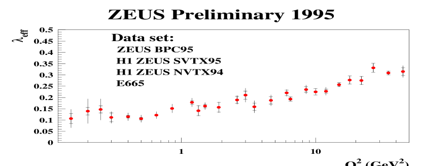
Figure 29: The behaviour with $Q^{2}$ of the exponent $\lambda_{eff}$ from fits of the form $F_{2}\sim x^{-\lambda_{eff}}$ at fixed $Q^{2}$ values and $x<$0.1.

The rise of the exponent (denoted in this figure as $\lambda_{eff}$) with $Q^{2}$ seems to be a smooth one. A warning is however in place at this point. The exponent is sensitive to the range in $x$ over which the fit is being carried out. There is not always a large enough lever arm in $x$ from lower energy data to get a good reliable fit for all values of $Q^{2}$. Thus further analysis is needed to give an accurate behaviour of the slope at the low $Q^{2}$ values.

There are quite a few parameterizations which attempt to describe the data both at low and at high $Q^{2}$ including the transition region. In figure 30 the $\gamma^{*}p$ total cross section $\sigma(\gamma^{*}p)$ is plotted as function of $W^{2}$ for fixed values of $Q^{2}$, including the total photoproduction cross section ($Q^{2}$ = 0). The curves are the results of the ALLM97 [47] parameterization which gives a good fit to all the available data over the whole kinematic region. The parameterization is based on a Regge motivated approach, similar to that used earlier by Donnachie and Landshoff [48], extended into the large $Q^{2}$ regime in a way compatible with QCD expectations. The transition from the Regge to the QCD regime can be seen in figure 31 which shows the $F_{2}$ data as function of $Q^{2}$ for fixed $x$ values, a comparison with the Regge based DL model, the QCD GRV(94) model and the ALLM97 parameterization which moves from the DL at low $Q^{2}$ to GRV at higher $Q^{2}$, following the data.

2.9 What have we learned about the proton?

To summarize this section let us recap what we have learned about the structure of the proton from the HERA data. There are two clear points that one can make:

• The density of partons increases with decreasing $x$. At $Q^{2}$ values of 10-20 GeV² and low $x$, the proton is dominated by gluons with a density of more than 20 gluons per unit of rapidity.

• The rate of increase of the parton density is $Q^{2}$ dependent. This dependence at high $Q^{2}$ is as expected from ‘hard’ interactions described by pQCD and at low $Q^{2}$, as coming from ‘soft’ interactions described by Regge phenomenology.

What does it imply as far as the actual picture of the structure of the proton is concerned? Can we say for instance that these dense partons are concentrated somewhere in the interior of the proton? We will come back to this and other questions at the end of the talk.

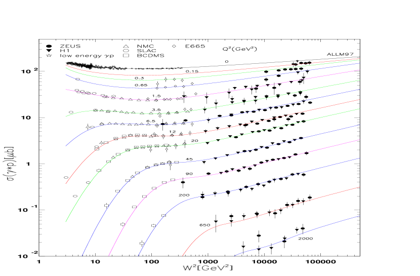
Figure 30: The $\gamma^{*}p$ total cross section $\sigma(\gamma^{*}p)$ as function of $W^{2}$ for fixed values of $Q^{2}$, including the total photoproduction cross section ($Q^{2}$ = 0). The curves are the results of the ALLM97 parameterization.

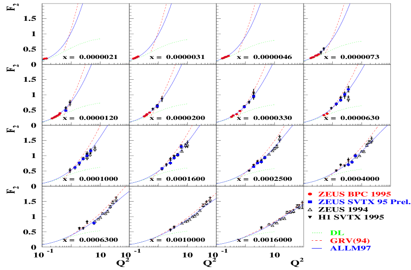
Figure 31: The behaviour with $Q^{2}$ of the exponent $\lambda$ from fits of the form $F_{2}\sim x^{-\lambda}$ at fixed $Q^{2}$ values and $x<$0.1.

3 The structure of the photon

In what follows, whenever we talk about a photon, we mean either a real photon or a quasi-real one. We will also discuss separately the structure of virtual photons. Let us recap what we said in the introduction about the photon structure. A high energy photon can develop a structure when interacting with another object. This happens because the photon can fluctuate into $q\bar{q}$ pairs and as long as the fluctuation time is large compared to the interaction time we can talk about the structure of the photon. Due to this phenomena a photon has a probability to interact as a photon directly with the other object, or first resolve itself into partons which subsequently take part in the interaction. We call the first case a direct photon interaction and the second one, a resolved photon interaction.

3.1 The behaviour of the photon structure function

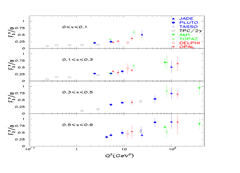
Figure 32: $F_{2}^{\gamma}$ as function of $Q^{2}$ for $x$ intervals as given in the figure.

The photon structure function $F_{2}^{\gamma}$ was measured in DIS type of $e^{+}e^{-}$ collisions as described in figure 8. From the structure function measurements one could obtain information on the parton distributions in the photon in a similar way to that of the proton, using the DGLAP equations. There is however one difference when viewing the DGLAP equations for the photon more closely. In the proton case, when considering the evolution equations, one takes into account the splitting of the partons in the following way: a quark of a given $x$ can split into a gluon and a quark, $q\to q+g$, both with lower $x$ but the sum of their $x$’s equal to the ‘parent’ $x$; a gluon can split into a pair of quark-antiquark, $g\to q+\bar{q}$; a gluon can split into two gluons, $g\to g+g$. However in the photon case one has in addition to all above splittings the possibility of a photon to split into a quark-antiquark pair, $\gamma\to q+\bar{q}$. This changes the DGLAP evolution equations from homogeneous to inhomogeneous ones. One of the consequences is that the scaling violations for the photon case are positive for all $x$ values, contrary to the proton case which had positive scaling violation for low $x$ and negative for high $x$. This can be seen in figure 32, where the photon structure function $F_{2}^{\gamma}$ is plotted as function of $Q^{2}$ for different $x$ intervals, and shows positive scaling violation in all $x$ bins. This behaviour should be contrasted to figure 24 for the proton case.

A compilation of the photon structure function, as presented at the Lepton Photon Symposium LP97 [49], is shown in figure 33 as function of $x$ for fixed $Q^{2}$.

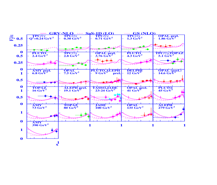
Figure 33: $F_{2}^{\gamma}$ as function of $x$ for fixed $Q^{2}$ as given in the figure. The curves are the expectations of different parameterizations of parton distributions in the photon.

The measurements have much larger errors than in the proton case. One of the main reasons is connected to the fact that it is difficult to determine the $x$ value of a given event in $\gamma\gamma$ interactions. The value of $x$ can in principle be calculated through the relation

$$x=\frac{Q^{2}}{Q^{2}+W^{2}}.$$ (25)

While $Q^{2}$ can be obtained by measuring the scattered electron (see figure 8), usually with an accuracy of better than 10 %, it is difficult to reconstruct the true $W$ value just from the measured final state kinematics. Another observation about figure 33 is that there is little data at low $x$. This is a consequence of not reaching, so far, high values of $W$ in $\gamma\gamma$ reactions. The curves in the figure are the calculations of some parameterizations [50] of parton distributions in the photon. While they give approximately the same results in the region where data exist, their predictions are quite different for the low $x$ region which is not constrained by data. Lately there has been much activity in the LEP community [51] to get more accurate data of $F_{2}^{\gamma}$ and extend the measurements to lower $x$ values (see also [52]).

3.2 Direct and resolved photon at HERA

Measurements of $F_{2}^{\gamma}$ constrain the quark distribution, while the gluons are badly determined. The first indications that gluons have to be present in the photon came from an analysis of jets in photon-photon interactions performed by the AMY collaboration [53]. They showed that the only way they can explain the data is by introducing some gluons in the photon. However it was at HERA that the picture of a direct and resolved photon was most clearly seen. At HERA? How does one study the structure of the photon at HERA? Did we not study the structure of the proton with the help of the photon in the previous section? As we said in the introduction to the present section, we consider now the structure of a quasi-real photon. In this case the probe is one of the large transverse momentum partons from the proton, and the photon plays the role of the probed target.

The diagrams in figure 34 describe what is meant in leading-order (LO) by direct and resolved photon in an example of photoproduction of dijets.

Figure 34: Examples of leading order QCD (a) ‘direct’ and (b) ‘resolved’ dijet production diagrams.

Diagram (a) describes the case in which all of the photon energy is involved in the dijet production. In diagram (b) the photon first resolves into partons; one of them interacts with a parton from the photon to produce a dijet while the rest remain as a photon remnant. In this case only part of the initial photon energy participates in the dijet production. If we denote by $x_{\gamma}$ the fraction of the photon energy participating in the dijet production, we expect $x_{\gamma}$ = 1 for the direct reaction and $x_{\gamma}<$ 1 for the resolved case. One can calculate an observable $x_{\gamma}^{obs}$ which will gives us a good approximation of the fraction $x_{\gamma}$,

$$x_{\gamma}^{obs}=\frac{E_{T}^{j1}e^{-\eta^{j1}}+E_{T}^{j2}e^{-\eta^{j2}}}{2E_{\gamma}}.$$ (26)

The transverse energies of the outgoing jets are denoted by $E_{T}^{ji}$ and their pseudorapidities  by $\eta^{ji}$.

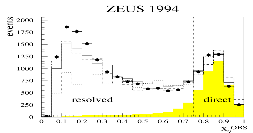
Figure 35: The $x_{\gamma}^{obs}$ distribution as obtained from photoproduction of dijet events. The shaded area are the expectations of the distribution of this variable from the generation of direct photon events. The dotted vertical line is the border of an operational definition of direct and resolved photon events.

Figure 35 displays the variable $x_{\gamma}^{obs}$ as measured by the ZEUS collaboration [54]. The data show a large enhancement at low $x_{\gamma}$ values coming from events in which only a small part of the photon energy participated in the production of the two jets. We called these resolved photon events in the above discussion. However, there is in addition a second peak around $x_{\gamma}^{obs}\approx$ 0.9, indicating that the whole of the photon participated in the dijet production, meaning it was a direct photon event. As we said above, $x_{\gamma}^{obs}$ is an estimator of $x_{\gamma}$ and therefore is somewhat smaller than 1. In order to see that the large $x$ enhancement indeed comes from direct photon interactions, such events were generated in a Monte Carlo program and the results are displayed as a shaded band in figure 35. It is clear from this that most of the large $x$ enhancement comes from direct photon events. How would one choose these events? We have a distribution in the figure and have to make an operational definition as to what we call direct and resolved events. The dotted line at $x_{\gamma}^{obs}$ = 0.75 is defined as the division line between direct ($>$ 0.75) and resolved ($<$ 0.75) events.

How can one check independently that this definition is sensible? Let us look again at the two diagrams in figure 34. In case of the direct photon diagram (also called ‘boson-gluon fusion’) the exchanged particle in the reaction $\gamma g\to qq$ is a quark, while in the resolved case, the exchange particle in the reaction $qg\to qg$ is a gluon. In case of the quark exchange, we have a spin $\frac{1}{2}$ propagator while in the gluon exchange case there is a spin 1 propagator. These different propagators lead to different angular distributions of the two outgoing quarks which are the ‘parents’ of the dijet. In case of the quark exchange one expects,

$$\frac{d\sigma}{d\cos\theta}\sim\frac{1}{1-|\cos\theta|},$$ (27)

while for the spin 1 exchange the angular distribution should be,

$$\frac{d\sigma}{d\cos\theta}\sim\frac{1}{(1-|\cos\theta|)^{2}}.$$ (28)

The quark exchange should dominate the direct photon events while the gluon exchange will dominate the resolved photon events. By using the above definition of the $x_{\gamma}^{obs}$ cut, one can choose samples of direct and resolved photon events and study their angular distribution. The results of this study [55] are displayed in figure 36.

Figure 36: The angular distribution $\frac{d\sigma}{d\cos\theta}$ of dijet events produced by resolved and by direct photon events. In (a) the data are compared to leading-order (LO) and next-to-leading-order (NLO) QCD calculations at the parton level. In (b) the comparison of the data is done at the hadron level with two Monte Carlo generators.

The data fulfill the expectations of our definition above. The events which were chosen as resolved photon events have a steeper angular distribution than the direct dijet events. The data are compared at two levels. The diagrams and the angular distribution considerations were done at the parton level, while the measured data are at the hadron level. In case of the jet the expectations are that the jet ‘remembers’ the direction of its ‘parent’ parton. Thus the comparison of the data is once done to a parton level calculation and then to a hadron level simulation. In figure 36(a) the comparison of the data is to a leading-order (LO) and to a next-to-leading-order (NLO) QCD calculation. In figure 36(b) the comparison is done with two Monte Carlo generators who give the angular distributions at the hadron level. The agreement with the data is very good in all cases. We can thus conclude that our direct and resolved definition using the $x_{\gamma}^{obs}$ cut is a reasonable one.

3.3 The gluon density in the photon

We have already said this but let us repeat: the structure function constrains the quarks. The information about the gluon distribution is indirectly obtained through the evolution equations. However the photon structure function data are not precise enough for a good determination of the gluon density in the photon.

Figure 37: The gluon density in the photon as function of $x_{\gamma}$ at a scale of 38 GeV². The different curves are the expectations of different parameterizations of parton distributions in the photon.

An interesting method to overcome this difficulty was carried out by the H1 collaboration [56]. They use the high transverse momentum charged tracks in photoproduction events to reconstruct the $x_{\gamma}$ distribution. Since the quark densities are constrained by the $F_{2}^{\gamma}$ measurements and thus relatively well known, their contribution to the $x_{\gamma}$ distribution are taken from the expectations of the photon parton parameterizations and are subtracted to give the gluon density as function of $x_{\gamma}$. The result of this analysis is shown in figure 37 for the case where the hard scale, taken from the average squared transverse momentum of all charged tracks, was 38 GeV². The data shows a rise of the gluon density with decreasing $x_{\gamma}$, a similar trend as in the proton case. The data of the analysis described above is compared to a similar analysis in which the $x_{\gamma}$ was reconstructed using dijet photoproduction events.The two results are consistent with each other. The data are also in general agreement with three parameterizations of the parton distributions in the photon (GRV-LO [57], LAC1-LO [58], SaS1D-LO [59]).

3.4 The structure of virtual photons

So far we discussed the structure of a real photon. Do virtual photons also have structure? The only measurement of the structure function of a photon with virtuality of about 0.4 GeV² was carried out by the PLUTO Collaboration [60] in $e^{+}e^{-}$ collisions at a probing scale of 5 GeV². The cross section of $e^{+}e^{-}$ interactions in which both leptons are detected is falling fast and thus such a measurement is difficult. At HERA however, one can study the structure of virtual photons by measuring the $x_{\gamma}$ distributions for events in different ranges of the photon virtuality $Q^{2}$. The presence of a structure of virtual photons will show itself in events having a low $x_{\gamma}$ value. This will signal resolved virtual photons (see discussion of figure 34).

The ZEUS collaboration [61] used data in three different ranges of $Q^{2}$. In the first, the scattered lepton was measured in the luminosity electron calorimeter, ensuring that the photon is quasi-real with a median $Q^{2}$ = $10^{-3}$ GeV². The second sample included events in which the scattered positron was measured in the BPC, yielding photons with virtuality in the region $0.1<Q^{2}<0.7$ GeV². In the third sample the scattered lepton was detected in the main calorimeter and was in the range $1.5<Q^{2}<4.5$ GeV².

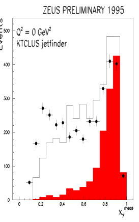
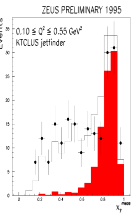
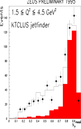
Figure 38: The $x_{g}amma$ distributions for three regions of $Q^{2}$ as displayed in the figure. The unshaded histograms are the sum of resolved and direct photon contributions as calculated from a LO Monte Carlo generator. The shaded histograms are only the LO direct photon contributions.

The dijets were used to calculate the value of $x_{\gamma}$ in each $Q^{2}$ region, results of which are displayed in figure 38. The data show the presence of resolved photon events in the low $x_{\gamma}$ region while the enhancement at high $x_{\gamma}$ is due to direct photon events. The histograms in the figures are the sum of resolved and direct photon contributions as calculated from a LO Monte Carlo generator. The shaded histograms are only the LO direct photon contributions.

Using the data and the operational definition of $x_{\gamma}<$ 0.75 as resolved photon events, one can calculate the ratio of resolved to direct photon events as function of the virtuality of the photon. This ratio is displayed in figure 40 and is decreasing with increasing $Q^{2}$. Note however that there is still an appreciable cross section of resolved photon events even at a virtuality of $Q^{2}$ = 4.5 GeV². It should be noted that in this study the minimum transverse energy $E_{T}$ of each of the two jets was 6.5 GeV², thus making sure that the probing scale (estimated by $E_{T}^{2}$) is much larger than the virtuality $Q^{2}$ of the probed photon.

Figure 39: The ratio of resolved to direct photon cross sections as a function of the photon virtuality $Q^{2}$.

Figure 40: The effective parton density of the photon as function of the squared of the parton transverse momentum $P_{t}^{2}$ for different values of $Q^{2}$ and $x_{\gamma}$. The lines are expectations of different parameterizations of parton distributions in the photon.

The H1 collaboration extracted in a similar study [62] an effective parton density of the virtual photon, shown in figure 40. Here too dijet events have been used in a wide range of the photon virtuality, $1.6<Q^{2}<80$ GeV², with the requirement that the probing parton transverse momentum $P_{t}^{2}$ is always much larger than $Q^{2}$. The effective parton density seems to rise with $P_{t}^{2}$ in all regions of $Q^{2}$, a behaviour which is in general agreement with expectations from parameterizations of parton distributions in the photon.

3.5 Who is probing whom?

The results we just obtained in the last subsection are somewhat alarming. We understand that a quasi-real photon has structure which is built during the interaction. Now we see that the same can be true for virtual photons, even with virtualities of some tens of GeV². How can a virtual photon develop a structure through fluctuation? Is the fluctuation time long enough? What about equation (16)? It turns out that the calculation of the fluctuation time for low $x$ gives [14, 22],

$$t_{f}\approx\frac{1}{2m_{p}x}.$$ (29)

So at low $x$ even a photon of virtuality $Q^{2}\sim 10^{3}$ GeV² can fluctuate! And here comes the alarming part: what are we measuring in a DIS interaction at low $x$? The simple picture of DIS is complicated at low $x$ by the long chain of gluon and quark ladders which describes the process in QCD. In this long chain of partons along the ladder, where does one draw the line? Does one study the structure of the proton? of the photon? of both? How should one interpret the DIS measurement? Who is probing whom?

It is clear that physics can not be frame dependent [63]. Thus it must be that both descriptions are correct and reflect the fact that cross sections are Lorentz invariant but time development is not [64]. This means that it shouldn’t matter whether one interprets the cross section measurements as yielding the proton or the photon structure function. By extracting one of them from the cross section measurement, there should be a relation allowing to obtain the other.

Here we have a problem. We have seen, at least as far as a real photon is concerned, that its structure function behaves very differently from that of the proton one. For instance, the $Q^{2}$ scaling violation is positive in the photon case for all values of $x$, while for the proton they change from positive to negative scaling violations as one moves to higher $x$ values. So how can the proton structure function $F_{2}^{p}$ and that of the photon, $F_{2}^{\gamma}$, be related?

Actually at low $x$ the two structure functions can be related. By assuming Gribov factorization [65] to hold also for a virtual photon one can show [66] that,

$$F_{2}^{\gamma}(x,Q^{2})=F_{2}^{p}(x,Q^{2})\frac{\sigma_{\gamma p}(W^{2})}{\sigma_{pp}(W^{2})}.$$ (30)

This last equation connects the proton and the real photon structure function at low $x$. By measuring one of them, the other can be determined through relation (30).

3.6 $F_{2}^{\gamma}$ at low $x$

Figure 41: The photon structure function as function of $x$ for fixed $Q^{2}$ values as indicated in the figure. The full points are the direct measurements and the open triangles are those obtained from $F_{2}^{p}$ through the Gribov factorization relation. The full line is the result of the present HO fit and the dashed line is that of the LO parameterization.

Relation (30) allows the use of well measured quantities like total cross sections and the proton structure function $F_{2}^{p}$ to predict the values of the photon structure function $F_{2}^{\gamma}$ in the region of low $x$ where equation (30) is expected to be valid. Since this is also the region where direct measurements of the photon structure function are difficult and not available, the use of (30) provides a way to ‘obtain’ $F_{2}^{\gamma}$ ‘data’ and use them as an additional source, on top of the direct measurements of $F_{2}^{\gamma}$, to constrain the parton distributions in the photon. This was done in LO in [68], where for the total cross sections of $\gamma p$ and $pp$ the DL [15] parameterization has been used. Recently [69] the same method was applied in a higher-order (HO) treatment and the results are displayed in figure 41. The directly measured photon structure function data appear as full points, while the data obtained through the use of the Gribov factorization relation are displayed as open triangles. All the low $x$ data coming from the proton structure function have been scaled to the value of $Q^{2}$ which is indicated in the figure. The solid curves are the results of the HO parameterization. For comparison we show as dashed lines the result of the LO parameterization which is very similar to the HO one, with the difference between the two growing as $Q^{2}$ increases.

3.7 Configurations of photon fluctuation

The photon can fluctuate into typically two configurations. A large size configuration will consist of an asymmetric $q\bar{q}$ pair with each quark carrying a small transverse momentum $k_{T}$ (fig. 42(a)). For a small size configuration the pair is symmetric, each quark having a large $k_{T}$ (fig. 42(b)). One expects the asymmetric large configuration to produce ’soft’ physics, while the symmetric one would yield the ’hard’ interactions.

In the aligned jet model (AJM) [67] the first configuration dominates while the second one is the ’sterile combination’ because of color screening. In the photoproduction case ($Q^{2}$ = 0), the small $k_{T}$ configuration dominates. Thus one has large color forces which produce the hadronic component, the vector mesons, which finally lead to hadronic non–perturbative final states of ’soft’ nature. The symmetric configuration contributes very little. In those cases where the photon does fluctuate into a high $k_{T}$ pair, color transparency suppresses their contribution.

Figure 42: Fluctuation of the photon into a $q\bar{q}$ pair in (a) asymmetric small $k_{T}$ configuration, (b) into a symmetric large $k_{T}$ configuration.

In the DIS regime ($Q^{2}\neq$ 0), the symmetric contribution becomes bigger. Each such pair still contributes very little because of color transparency, but the phase space for the symmetric configuration increases. However the asymmetric pair still contribute also to the DIS processes. In fact, in the quark parton model (QPM) the fast quark becomes the current jet and the slow quark interacts with the proton remnant resulting in processes which look in the $\gamma^{*}p$ frame just like the ’soft’ processes discussed in the $Q^{2}$ = 0 case. So there clearly is an interplay between soft and hard interactions also in the DIS region.

3.8 What have we learned about the photon?

We can summarize our present knowledge about the structure of the photon in the following way:

• Real photons have structure which is developed in the interactions through the fluctuation of the photon into a $q\bar{q}$ pair. There are clear signs of the direct and resolved photon processes at HERA.

• The photon and proton structure functions can be related at low $x$.

• Virtual photons also develop a structure.

• The nature of the interaction, soft or hard, is determined by the configuration of the photon fluctuation. This creates regions in physics in which there is an interplay between soft and hard interactions.

4 The structure of the Pomeron

The soft and hard interplay mentioned in the last section brings us in a natural way to the subject of diffraction. We know from hadron-hadron interactions that diffraction [71] is a ‘soft’ phenomena. It is described by the exchange of the Pomeron trajectory. We already mentioned earlier that Donnachie and Landshoff [15] determined this trajectory as,

$$\alpha_{IP}(t)=1.08+0.25t.$$ (31)

The intercept was determined from a fit to all hadron-hadron total cross section data and the slope $\alpha^{\prime}_{IP}$ was determined [70] from $pp$ elastic scattering data. What does HERA tell us about diffraction? Is it a soft phenomenon described by Regge phenomenology? Is it a hard process calculable in pQCD? Or both? Let us first look at inclusive studies in DIS.

4.1 Inclusive studies in diffractive DIS processes.

We have seen in the introduction that the discovery of large rapidity gap events in DIS came as a surprise. The reason was that our intuition about DIS is based on the quark-parton model and on the QCD evolution. It is difficult to see how in such a picture the struck parton will not radiate gluons so as to create large rapidity gap events which are not exponentially suppressed. That is why none of the Monte-Carlo generators which were written for DIS physics at HERA included diffractive type of events. On the other hand, from the proton rest frame point of view, one could naturally expect large rapidity gap events for example in the aligned-jet model (shown to hold also in QCD [72]).

However, even before HERA started producing data, Ingelman and Schlein [73] hypothesized that the Pomeron has a partonic structure like any other hadron. They suggested that the structure of the Pomeron can be studied in a similar DIS process as for the proton, in the reaction $ep\to epX$ which was described in figure 11. That diagram is very similar to the one of a $\gamma^{*}\gamma$ interaction in which the process at the lepton vertex is looked upon as a source of photons and is factorized in the calculation of the $\gamma^{*}\gamma$ cross section of the diagram. Also in the Pomeron case one assumes that the proton acts as a source of a flux of Pomerons which are probed by the $\gamma^{*}$. In the interpretation of the process as probing the structure of the Pomeron one thus assumes that the cross section for the process $ep\to epX$ can be factorized into the contribution coming from $e{IP}\to eX$ and the one from the vertex $p\to{IP}p$ which produces the flux of Pomerons.

The assumption of factorization is used to develop the whole formalism of the Pomeron structure function which can be subjected to the same DGLAP equations as the proton, given the fact that the QCD factorization theorem has been proven [74] to hold also in inclusive DIS diffractive processes. These inclusive processes have been measured by both the H1 [75] and the ZEUS [76] collaborations and the cross section has been analyzed as a product of the Pomeron flux and the Pomeron structure function. Contrary to the case of the proton, the scaling violation of the Pomeron structure function did not change sign when moving from low to high $\beta$ values. The variable $\beta$ for the Pomeron case has a similar meaning as the Bjorken $x$ for the proton.

From the results of such a factorization analysis one gets two main results. From the flux factor one gets information about the Pomeron trajectory. From the Pomeron structure function QCD analysis one gets a determination of the parton distributions in the Pomeron. Let us start with the latter; in figure 44 the resulting parton distributions at different $Q^{2}$ values are plotted as function of the fraction $z$ of the Pomeron momentum carried by the struck parton.

Figure 43: Quark and gluon momentum distributions in the Pomeron as a function of the fraction $z$ of the Pomeron momentum, for different fits to the measurements of the diffractive structure function in DIS. The results are evolved to different $Q^{2}$ values as denoted in the figure.

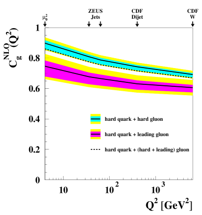
Figure 44: Fraction $c_{g}$ of the Pomeron momentum carried by gluons as a function of $Q^{2}$, determined from a NLO QCD fit to the diffractive structure function in DIS and the diffractive dijet cross section in photoproduction.

The plot shows results of two different fits. However without going into details, one can clearly see that the gluons carry a dominant part of the Pomeron momentum. This can also be seen from figure 44 where the fraction $c_{g}$ of the Pomeron momentum carried by the gluons, as obtained from a NLO QCD fit, is plotted as a function of $Q^{2}$. In spite of the slight decrease with $Q^{2}$, the gluons seem to carry about 60-80% of the Pomeron momentum.

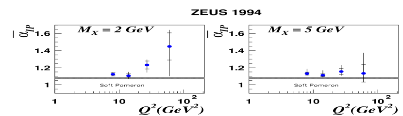
Figure 45: The value of the $t$ averaged Pomeron trajectory, $\overline{\alpha_{IP}}$, as a function of $Q^{2}$ and for two mass ranges $M_{X}$ as derived from the fit to the $W$ dependence of the cross section. The shaded area is the result expected for the soft Pomeron exchange assuming $\alpha^{\prime}_{IP}$ = 0.25 GeV^-2.

As for the Pomeron trajectory, the H1 [75] analysis yields the following result, $\alpha_{IP}(0)=1.203\pm 0.020({\rm stat})\pm 0.013({\rm syst})^{+0.030}_{-0.035}({\rm model})$, a value which seems to be $Q^{2}$ independent in the range $0.4<Q^{2}<$ 75 GeV². The ZEUS [76] analysis of inclusive diffraction processes is limited to diffractive masses $M_{X}<$ 15 GeV. From the study of the energy dependence of the diffractive cross section, a $t$-averaged Pomeron trajectory $\overline{\alpha_{IP}}$ is obtained. The results are displayed in figure 45 as a function of $Q^{2}$ for two regions of $M_{X}$. Though there seems to be some signs for a $Q^{2}$ dependence in the low mass region, a higher statistics measurement at higher $Q^{2}$ is needed for firm conclusions. One can however conclude that the trajectory is higher than that expected from soft processes.

What can one conclude from these results? The inclusive DIS diffractive cross section seems to be factorizable and one obtains a partonic picture of the Pomeron in which gluons carry the dominant fraction of the Pomeron momentum. The resulting Pomeron trajectory seems to be different than that of the DL soft Pomeron. Actually if the trajectory is $Q^{2}$ dependent, it is not a Regge pole. The $Q^{2}$ dependence is a feature of pQCD, indicating the important role of hard physics. What does it mean as far as the nature of the diffractive process is concerned? Are we seeing a hard diffractive process? Is it all hard? Is there here too an interplay of hard and soft processes?

4.2 Exclusive diffractive vector meson production

We will try to look into the questions raised in the earlier subsection by studying simpler systems. Actually we shall start with the most inclusive process - the total cross section. We have already seen that Regge phenomenology expects $\sigma_{tot}\sim s^{\alpha(0)-1}$ and therefore for a soft process dominated by the DL Pomeron one expects,

$$\sigma_{tot}\sim s^{0.08}\sim W^{0.16}.$$ (32)

This behaviour is indeed found to hold for $\sigma_{tot}(\gamma p)$ as we have shown in figure 10 and therefore making it a predominantly soft process.

What does one expect in this picture for the behaviour of the elastic  cross section with energy? In photoproduction the elastic cross section refers to vector meson production, as described by the diagram in figure 47. The photon first fluctuates into a virtual vector meson which scatters elastically off the proton. This is a diffractive process dominated by a Pomeron exchange.

Figure 46: A diagram describing diffractive production of vector mesons by an exchange of a Pomeron.

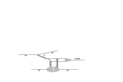
Figure 47: A diagram describing diffractive production of vector mesons as two gluon exchange.

In this picture, the use of the optical theorem would predict that the elastic cross section $\sigma_{el}$ should behave as,

$$\sigma_{el}\sim W^{4\alpha(t)-4}\sim W^{0.22}.$$ (33)

The power of $W$ is less than 0.32 because of the slope of the Pomeron trajectory, taken here as $\alpha_{IP}^{\prime}$ = 0.25 GeV^-2.

How would one describe the production of vector mesons in a hard process? The virtual photon fluctuates into a symmetric $q\bar{q}$ pair which exchange two gluons with the proton and turn into a vector meson [77, 78]. This is described diagrammatically in figure 47. In this case the $W$ behaviour of the cross section is dictated by the $x$ behaviour of the gluon density and since the latter shows a steep increase as $x$ decreases, one thus expects a steep increase of the cross section as $W$ increases. Can we quantify this? We saw that at low $x$ the proton structure function behaves like $F_{2}^{p}\sim x^{-\lambda}$ and since at low $x$ the rise is driven by the gluons, this is also the behaviour of the gluon density. Translated into $W$ dependence, we expect for a hard process,

$$\sigma_{el}\sim W^{4\lambda}.$$ (34)

Since we have seen in the proton section that $\lambda$ is $Q^{2}$ dependent, this means that we expect the $W$ dependence of a hard process also to be $Q^{2}$ dependent.

What is the experimental situation? The cross section data for the elastic vector meson photoproduction are displayed in figure 48. For comparison also the data of $\sigma_{tot}(\gamma p)$ are shown together with the line describing the $W^{0.16}$ behaviour.

Figure 48: The elastic photoproduction cross section of vector mesons as function of $W$. The total photoproduction cross section $\sigma_{tot}$ is also shown for comparison.

The light vector mesons $\rho^{0}$, $\omega$ and $\Phi$ have an energy dependence which is well described by $W^{0.22}$ as expected from a diffractive process mediated by the soft Pomeron. This behaviour changes drastically for the $J/\psi$ vector meson, where the $W$ behaviour is much steeper, $\sim W^{0.8}$, indicative of a hard process. What has happened? Why this change from a soft behaviour to a hard one? In the total cross section case, the processes are dominated by low scales. The same is true for the light vector mesons. However in case of the $J/\psi$, the heavy quark mass produces a large enough scale for the reaction to become hard. Does it mean that the process is completely calculable in pQCD? We will return to this question later.

Following the above logic, we can now check if we observe a steep $W$ dependence in other exclusive processes where a hard scale is present. In case of the light vector meson, the hard scale has to be provided by the virtuality of the photon.

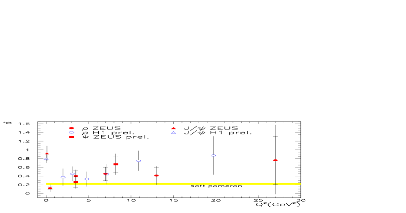
Figure 49: The power $\delta$ of the energy dependence of the cross section of diffractive vector meson production, $\sigma\sim W^{\delta}$, as function of $Q^{2}$ for different vector mesons, as indicated in the figure.

The elastic (exclusive) cross section data have been fitted to the expression $\sigma\sim W^{\delta}$. In order to avoid normalization problems in comparing data from different experiments, the fits of the photoproduction $J/\psi$ data as well as that of the DIS exclusive vector meson data was done by using only the HERA data. The results of the fit are displayed in figure 49 which shows the dependence of $\delta$ on $Q^{2}$. For the $\rho^{0}$ and the $\Phi$ vector mesons, the value of $\delta$ shows the tendency of an increase with $Q^{2}$, though the errors on $\delta$ are still quite large. One sees at $Q^{2}$ = 0 the high value of $\delta$ for the case of the $J/\psi$. At higher $Q^{2}$ there is not enough HERA data on $J/\psi$ to perform a $W$-dependence fit for obtaining the value of $\delta$. However the higher $Q^{2}$ $J/\psi$ data can be described with the same value of $\delta$ as the one obtained at $Q^{2}$ = 0.

4.3 Gribov diffusion

The conclusion from the last figure seems to be that the presence of a large scale ($\sim$ 10-20 GeV²) causes a process to become hard. We have however to define more accurately what we mean by a hard process [79]. A process is said to be hard if it is driven by parton interactions and therefore calculable in pQCD. One of the requirements is indeed a steeper $W$ dependence. Is this enough? We saw that $\sigma_{tot}(\gamma^{*}p)$ has a steep behaviour as $Q^{2}$ increases. Are all processes at higher $Q^{2}$ calculable in pQCD? Can we calculate the complete process of $J/\psi$ photoproduction in pQCD?

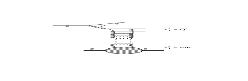
Figure 50: A diagram describing a gluon ladder in a diffractive process.

Let us look again at the diagram describing two gluon exchange in figure 47. The virtual photon fluctuates into two high $k_{T}$ quarks. Although in the diagram there are only two gluons getting down to the proton, we actually have a whole ladder due to the large rapidity range available at these high $W$ energies (see figure 50). During the trip from the virtual photon vertex down to the proton, the average $k_{T}$ of the gluons gets smaller, the configuration larger and we get into the region of low $k_{T}$ physics governed by non-perturbative QCD. This process is called Gribov diffusion [23](see also [80]). Thus a process can start off as a hard process at the photon vertex but once it arrives at the proton it gets a ‘soft’ element which makes the process non calculable in pQCD. The average $k_{T}$ of the partons in the process can be estimated by the slope of the trajectory since $\alpha^{\prime}\sim 1/<k_{T}>$. Is Gribov diffusion always present? If the answer is positive, we will always have a ‘soft’ element in the process which will prevent a full pQCD calculation. One way to look for an answer is to determine the Pomeron trajectory in a given process and look at the value of the slope of the trajectory. For a hard process as defined above we would expect $\alpha^{\prime}\ll$ 0.25 GeV^-2.

4.4 Determination of the Pomeron trajectory.

Regge phenomenology [81] connects the differential cross section of a two-body process with the leading exchanged trajectory as follows,

$$\frac{d\sigma}{dt}=f(t)(W^{2})^{[2\alpha(t)-2]},$$ (35)

where $f(t)$ is a function of $t$ only. Thus by studying the $W$ dependence of $d\sigma/dt$ at fixed $t$ values, one can determine $\alpha(t)$. If in addition the trajectory is assumed to be linear,

$$\alpha(t)=\alpha(0)+\alpha^{\prime}t,$$ (36)

the intercept and slope of a trajectory can be obtained by fitting the measured $\alpha(t)$ values to a linear form.

In order to use this method for the determination of the Pomeron trajectory, one needs to find processes where the Pomeron is the dominating exchanged trajectory. Furthermore, for a good determination of the values of $\alpha(t)$ one needs data in a large range in $W$ at a given $t$. The new HERA data allows such an analysis for the reactions $\gamma p\to\rho^{0}p$, $\gamma p\to\Phi p$, and $\gamma p\to J/\psi p$. The elastic photoproduction of $\rho^{0}$ is dominated by Pomeron exchange for $W>$ 8 GeV. For the $\Phi$ and $J/\psi$ elastic photoproduction reaction, the Pomeron is the only possible trajectory which one can exchange and thus one can use also the low $W$ data (of course after moving far enough above threshold effects).

The determination of the Pomeron trajectory in the elastic photoproduction of $\rho^{0}$, $\Phi$ and $J/\psi$ was carried out by the ZEUS collaboration [82]. Figure 51 shows the differential cross section data used in this analysis for the three vector mesons. At each $t$ value a fit to expression (35) was performed and a value for $\alpha(t)$ was obtained. These values are shown in figure 52. The resulting trajectories are,

• $\gamma p\to\rho^{0}p$:      $\alpha(t)=(1.097\pm 0.020)+(0.163\pm 0.035)t$,

• $\gamma p\to\Phi p$:      $\alpha(t)=(1.083\pm 0.010)+(0.180\pm 0.027)t$,

• $\gamma p\to J/\psi p$:    $\alpha(t)=(1.175\pm 0.026)+(0.015\pm 0.065)t$.

The following observations can be made: in case of the light vector mesons $\rho^{0}$ and $\Phi$ the intercepts are in good agreement with the DL value of 1.08. The slopes, however, are significantly different from the value of 0.25 GeV^-2 but still far enough from 0 in order to count as ‘soft’ processes in which Gribov diffusion is present.

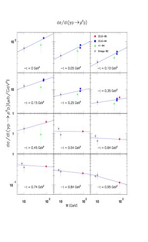
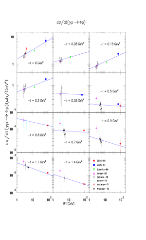
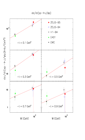
Figure 51: Fits to $d\sigma/dt\sim(W^{2})^{2\alpha(t)-2}$ for the reactions $\gamma p\to\rho^{0}p$ (left figure), $\gamma p\to\phi p$ (center figure) and $\gamma p\to J/\psi p$ (right figure).

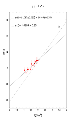
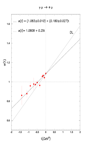
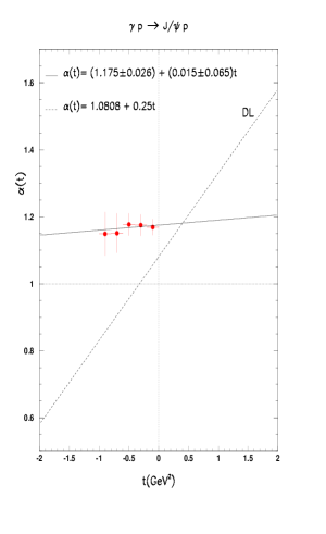
Figure 52: Determination of the Pomeron trajectory from the reactions $\gamma p\to\rho^{0}p$ (left figure), $\gamma p\to\phi p$ (center figure) and $\gamma p\to J/\psi p$ (right figure). In each of the three figures, the dots are the values of the trajectory as determined in the earlier figure and the full line is the result of a linear fit to these values. The Pomeron trajectory as determined by DL is shown for comparison as a dashed line.

In case of the $J/\psi$ the value of the slope is close to 0, as was already shown previously [83]. This indicates that for this reaction Gribov diffusion is unimportant in the present $W$ range. In other words, for the process $\gamma p\to J/\psi p$ the average $k_{T}$ of the partons involved in the exchange remains large and therefore the process is a ‘hard’ one, governed by the so-called ‘perturbative Pomeron’ and fully calculable in perturbative QCD.

4.5 Universal Pomeron?

The results of the last subsection lead us to question the universality of the Pomeron trajectory. If all data are interpreted in terms of the exchange of a Pomeron trajectory, we need as many trajectories as reactions. In the DIS region the $\sigma_{tot}(\gamma^{*}p)$ data can not be described by a $Q^{2}$ independent intercept. Whenever there is a large scale present, the $W$ dependence is steeper than expected from the DL Pomeron. The direct determination of the Pomeron trajectory indicates that even in processes which are shown to be of a predominantly ‘soft’ nature, the concept of a universal Pomeron is not borne out by the data.

We can try again to look at the large rapidity gap processes from the point of view of the different configurations into which the photon fluctuates. The small configuration enables to resolve partons in the proton, while the large configuration does not. The exchanged chain of partons, responsible for the strong interactions between the partons at the photon and those at the proton vertex, turn out to be predominantly gluons in both cases. However because of the different initial configuration of the photon fluctuation, there is no reason why their behaviour should be identical in both cases. There are many theoretical models, inspired by this picture, which attempt to describe the diffractive processes and the reader is referred to a summary in [84].

4.6 What have we learned about the Pomeron?

It is a bit difficult to summarize our knowledge about the Pomeron as presented in this section. If indeed it is not a universal concept then it is not clear what is the meaning of the results described above. Let us nevertheless list the main points:

• There are processes in DIS reactions leading to large rapidity gap events. These events are interpreted as diffractive reactions in which a Pomeron is being exchanged. When viewed as a DIS on an Ingelman-Schlein type of Pomeron, most of its momentum is carried by gluons. The intercept of such a Pomeron is different from the DL Pomeron.

• The properties of the Pomeron exchanged in elastic photoproduction of $J/\psi$ is also different from the DL Pomeron. Its intercept is larger, while it slope is much smaller than that of the DL Pomeron.

• The concept of a universal Pomeron is not borne out even by data coming from ‘soft’ processes.

5 Some simple-minded questions

We discussed the structure of the proton, the photon and the Pomeron. Let us start from the end. We know very little about the Pomeron. We know some of its quantum numbers: it has charge conjugation $C$ = +, it has positive parity $P$ = +, it has zero isospin $I$ = 0. What is its mass? We do not know. Is it a particle? We do not know. Are there particles lying on the Pomeron trajectory? There are some suggestions that there might exist a glueball candidate which could be on the Pomeron trajectory. Can we however talk about a universal trajectory given the different slopes and intercepts one seems to measure?

We know much more about the photon. It is an elementary gauge vector boson with definite spin, parity, charge conjugation $J^{PC}=1^{--}$. We are talking about the structure of the photon, though we understand that this structure is built up during the interaction. We thus talk about the photon structure function, parton distributions in the photon and understand that when it interacts with another hadron it has a probability to either interact with it directly (direct photon) or first turn into a state where it is composed of partons which then interact with the hadron (resolved photon). Although this picture is borne out by experimental data we still have some difficulty with the concept of the structure of the photon. The photon is not a particle that we can stop and look at its inside.

This brings us to the proton. Here the concept of the structure of the proton comes very naturally. The DIS experiments show clearly that the proton is composed of partons. How many partons are there in the proton? We don’t know, but we know that the higher we go in energy the density of these partons increases. Where in the proton are these partons located? Are they spread over the proton? Are they concentrated in a small part of the proton? What kind of experiment should we do to get some answer to this? We always say that DIS is just the continuation of Rutherford’s experiment. Well, he found that the nucleus is concentrated in a very small part of the Atom. What can we say about the partons inside the proton? Lonya Frankfurt’s answer [64] was that we have first to go to the proton rest frame. The reason is that the infinite momentum frame picture does not give direct information on the space location of the partons. This is because the light-cone description of the Feynman parton model does not explore the space-time location of partons at all. Within the infinite momentum frame description the variable $x$ has no direct relation to the space coordinate of a parton but is related to a combination of the energy and momentum of a parton.

On the contrary, the proton rest frame picture contains rather direct information about the location of partons in space-time. The key formula which relates both descriptions is that derived by Ioffe [14],

$$l=\frac{1}{2m_{p}x}\approx\frac{0.1\ {\rm fm}}{x},$$ (37)

giving the relation between Bjorken-$x$ and the distance $l$ in the direction of the exchanged photon. It follows from equation (37) that partons with $x>$ 0.1 are in the interior of the proton. All partons with $x<$ 0.1 have no direct relation to the structure of the proton. They do not belong to the proton ! In this picture all the sea quarks found at small $x$ are to a large extent the property of the photon wave function. Thus the popular comparison which I have used here with the Rutherford experiment is wrong for the HERA kinematics, though it was right to do so for the early SLAC DIS experiment which obtained data for $x>$ 0.1. Does this mean that in order to learn from HERA about the structure of the proton we should concentrate on the high $x$ physics?

The above argumentation actually suggests that the study of the low $x$ region will improve our knowledge about the details of the interaction. In order to find new features about the structure of the proton we should look into the high $x$ region with better resolution. The HERA high luminosity upgrade program will provide this opportunity.

Following the confusing questions above I find that the best way to finish this talk is with a quotation which I found in the book of Yndurain [85]. Alphonse X (The Wise, 1221–1284), who was King of Castillo and Leon, had the Ptolemaic system of epicycles explained to him. His reaction was the following:

‘If the Lord Almighty had consulted me before embarking upon creation, I should have recommended something simpler.’

6 Acknowledgment

It is a pleasure to acknowledge fruitful discussions with Halina Abramowicz, Yuri Dokshitzer, Lonya Frankfurt and Mark Strikman. Many thanks to Vladimir Petrov and the local organizing committee for inviting me to this pleasant and special workshop.

This work was partially supported by the German–Israel Foundation (GIF), by the U.S.–Israel Binational Foundation (BSF) and by the Israel Science Foundation (ISF).

References

- [1] For an excellent textbook on this subject see E. Leader, E. Predazzi, An introduction to gauge theories and modern particle physics, Cambridge University Press, 1996.
- [2] F. Halzen, A.D. Martin, Quarks and Leptons: An introductory course in modern particle physics, Wiley & Sons, 1984.
-
[3]
SLAC-MIT Collab, E.D. Bloom et al., Phys. Rev. Lett. 23 (1969) 930;
M. Breidenbach et al., Phys. Rev. Lett. 23 (1969) 935. - [4] CDHS Collab., J.G.H. De Groot et al., Zeit. Phys. C1 (1979) 143.
-
[5]
B.H. Wiik, Electron-proton colliding beams, the
physics program and the machine, Proc. 10th SLAC Summer
Institute, p. 233, 1982;
G.A. Voss, Proc. First Euro Acc. Conf., Rome, p 7, 1988. - [6] L.W. Whitlow et al., Phys. Lett. B282 (1992) 475.
- [7] BCDMS Collab., A.C. Benvenuti et al., Phys. Lett. B223 (1989) 485.
- [8] E665 Collab., M.R. Adams et al., Phys. Rev. D54 (1996) 3006.
- [9] NMC Collab., M. Arneodo et al., Nucl. Phys. B483 (1997) 3.
-
[10]
H1 Collab., I. Abt et al., Nucl. Phys. B407 (1993) 515;
T. Ahmed et al., Nucl. Phys. B439 (1995) 471;
T. Ahmed et al., Nucl. Phys. B470 (1996) 3;
C. Adloff et al., Nucl. Phys. B497 (1997) 3. -
[11]
ZEUS Collab., M. Derrick et al.,
Phys. Lett. B316 (1993) 412;
M. Derrick et al., Zeit. Phys. C65 (1995) 379;
M. Derrick et al., Zeit. Phys. C69 (1995) 607;
M. Derrick et al., Zeit. Phys. C72 (1996) 399;
J. Breitweg et al., Phys. Lett. B407 (1997) 432;
J. Breitweg et al., ZEUS results on measurement and phenomenology of at low and low , DESY 98-121, 1998. - [12] L.N. Hand, Phys. Rev. 129 (1963) 1834.
- [13] J.J. Sakurai, Ann. Phys. (NY) 11 (1960) 1.
-
[14]
B.L. Ioffe, Phys. Lett. B30 (1969) 123.
See also V.N. Gribov, B.L. Ioffe, I.Ya. Pomeranchuk, Sov. J. Nucl. Phys. 2 (1966) 549;
B.L. Ioffe, JETP Lett. 9 (1969) 97; JETP Lett. 10 (1969) 90;
V.N. Gribov, Sov. Phys. JEPT 30 (1970) 709. - [15] A. Donnachie, P.V. Landshoff, Phys. Lett. B296 (1992) 227.
- [16] I.Ya. Pomeranchuk, Sov. Phys. JEPT 7 (1958) 499.
- [17] H1 Collab., T. Ahmed et al., Phys. Lett. B299 (374) .
- [18] ZEUS Collab., M. Derrick et al., Phys. Lett. B293 (465) .
- [19] H. Abramowicz et al., Phys. Lett. B269 (1991) 465.
- [20] ZEUS Collab., M. Derrick et al., Phys. Lett. B315 (1993) 481.
- [21] H1 Collab., T. Ahmed et al., Nucl. Phys. B429 (1994) 477.
- [22] H. Abramowicz, L. Frankfurt, M. Strikman, Surveys in High Energy Phys. 11 (1997) 51.
- [23] V.N. Gribov, JETP Lett. 41 (1961) 667.(Reprinted in Regge theory of low- hadronic interactions, L. Caneschi (ed.) pp. 22-23).
- [24] For a recent review see E. Levin, An introduction to Pomerons, DESY 98-120, 1998.
- [25] D.R.O. Morrison, Phys. Rev. 165 (1968) 1699.
- [26] For a recent review on HERA physics, see H. Abramowicz, A. Caldwell, HERA Physics, to be published in Review of Modern Physics.
- [27] ZEUS Collaboration, J. Breitweg et al., Measurement of high- charged-current DIS cross sections at HERA, paper 751 submitted to the XXIX International Conference on High Energy Physics, Vancouver, 23-29 July, 1998.
- [28] Particle Data Group, R.M. Barnett et al., Europ. Phys. J. C3 (1998) 1.
- [29] H1 Collab., C. Adloff et al., Zeit. Phys. C74 (1997) 191.
- [30] ZEUS Collab., J. Breitweg et al., Zeit. Phys. C74 (1997) 207.
- [31] B. Straub, New results on neutral and charged current scattering at high from H1 and ZEUS, XVIII Int. Symp. Lepton Photon Interactions, Hamburg, 1997.
- [32] For a recent review see G. Wolf, Surveys in High Energy Phys. 12 (1998) 1.
- [33] H1 Collaboration, Measurement of neutral and charged current cross sections at high , paper 533 submitted to the XXIX International Conference on High Energy Physics, Vancouver, 23-29 July, 1998.
- [34] ZEUS Collaboration, J. Breitweg et al., Measurement of high- neutral-current DIS cross sections at HERA, paper 752 submitted to the XXIX International Conference on High Energy Physics, Vancouver, 23-29 July, 1998.
- [35] CTEQ Collab., H.L. Lai et al., Phys. Rev. D55 (1997) 1280.
- [36] J.C. Collins, D.E. Soper, G. Sterman, Nucl. Phys. B261 (1985) 104.
-
[37]
V.N. Gribov, L.N. Lipatov, Sov. J. Nucl. Phys. 15 (1972) 438,675;
G. Altarelli, G. Parisi, Nucl. Phys. B126 (1977) 298;
Yu.L. Dokshitzer, Sov. Phys. JEPT 46 (1977) 641. -
[38]
E.A. Kuraev, L.N. Lipatov, V.S. Fadin, Sov. Phys. JEPT 44 (1976) 443;
E.A. Kuraev, L.N. Lipatov, V.S. Fadin, Sov. Phys. JEPT 45 (1977) 199;
Y.Y. Balitski, L.N. Lipatov, Sov. J. Nucl. Phys. 28 (1978) 822. - [39] For a recent review on the nucleon structure function, see A.M. Cooper-Sarkar, R. Devenish, A. De Roeck, Int. J. Mod. Phys. A13 (1998) 3385.
- [40] A.D. Martin et al., Parton distributions: a new global analysis, hep-ph/9803445, 1998.
- [41] H1 Collab., C. Adloff et al., Nucl. Phys. B497 (1997) 3.
- [42] M. Gluck, E. Reya, A. Vogt, Zeit. Phys. C67 (1995) 433.
- [43] A. Capella et al., Phys. Lett. B337 (1994) 358.
- [44] J. Kwiecinski, B. Badelek, Zeit. Phys. C43 (1989) 251; Phys. Lett. B295 (1992) 263.
- [45] K. Adel, F. Bareiro, F.J. Yndurain, Nucl. Phys. B495 (1997) 221.
- [46] A. Levy, Low- Physics at HERA, in Lectures on QCD, F. Lenz, H. Griesshammer, D. Stoll (eds.), pp. 347-477, Springer-Verlag 1997; DESY 97–013 (1997).
- [47] H. Abramowicz, A. Levy, The ALLM parameterization of : an update, DESY 97–251, hep-ph/9712415 (1997).
- [48] A. Donnachie, P.V. Landshoff, Nucl. Phys. B244 (1984) 322.
- [49] S. Soldner-Rembold, The structure of the photon, XVIII Int. Symp. Lepton Photon Interactions, Hamburg, 1997.
-
[50]
M. Gluck, E. Reya, A. Vogt, Phys. Rev. 46 (1992) 1973;
G.A. Schuler, T. Sjöstrand, Zeit. Phys. C68 (1995) 607;
L.E. Gordon, J.K. Storrow, Zeit. Phys. C56 (1992) 307. -
[51]
DELPHI Collab., P. Abreu et al.,
Zeit. Phys. C69 (1995) 209;
OPAL Collab., K. Ackerstaff et al., Zeit. Phys. C74 (1997) 33;
K. Ackerstaff et al., Phys. Lett. B411 (1997) 387;
ALEPH Collab., Submitted to Photon ’97 and LP97;
L3 Collab., M. Acciarri et al., Phys. Lett. B436 (1998) 403. - [52] M. Krawczyk, A. Zemburski, M. Staszel, Survey of recent data on photon structure functions and resolved photon processes, DESY 98-013, 1998.
- [53] AMY Collab., R. Tanaka et al., Phys. Lett. B277 (1992) 215.
- [54] ZEUS Collab., M. Derrick et al., Europ. Phys. J. C1 (1998) 109.
- [55] ZEUS Collab., M. Derrick et al., Phys. Lett. B384 (1996) 401.
- [56] H1 Collab., C. Adloff et al., Charged Particle Cross Sections in Photoproduction and Extraction of the Gluon Density in the Photon, DESY-98-148 (1998).
- [57] M. Gluck, E. Reya, A. Vogt, Phys. Rev. 46 (1992) 1973.
- [58] H. Abramowicz, K. Charchula, A. Levy, Phys. Lett. B269 (1991) 458.
- [59] G.A. Schuler, T. Sjöstrand, Phys. Lett. B376 (1996) 193.
- [60] PLUTO Collab., Ch. Berger et al., Phys. Lett. B142 (1984) 119.
- [61] ZEUS Collab., J. Breitweg et al., Dijet cross sections in interactions using real and virtual photons at HERA, paper 816 submitted to the XXIX International Conference on High Energy Physics, Vancouver, 23-29 July, 1998.
- [62] H1 Collab., Measurement of di-jet cross-sections in low deep-inelastic scattering processes at HERA and extraction of an effective parton density of the virtual photon, paper 544 submitted to the XXIX International Conference on High Energy Physics, Vancouver, 23-29 July, 1998.
- [63] J.D. Bjorken Proceedings of the International Workshop on DIS and related subjects, Eilat, 1994, p. 151.
- [64] L. Frankfurt, private communication.
- [65] V.N. Gribov, L.Ya. Pomeranchuk, Phys. Rev. Lett. 8 (1962) 343.
- [66] A. Levy, Phys. Lett. B404 (1997) 369.
- [67] J.D. Bjorken, Proceedings of the International Symposium on Electron and Photon interactions at High Energies, Cornell, 1971, p. 281.
- [68] H. Abramowicz, E. Gurvich, A. Levy, Phys. Lett. B420 (1998) 104.
- [69] H. Abramowicz, E. Gurvich, A. Levy, Next to leading order parton distributions in the photon from and scattering, paper 684 submitted to the XXIX International Conference on High Energy Physics, Vancouver, 23-29 July, 1998.
-
[70]
G. Jaroszkiewicz, P.V. Landshoff, Phys. Rev. D10 (1974) 170;
P.D.B. Collins, F.D. Gault, A. Martin, Nucl. Phys. B80 (1974) 135. - [71] For a recent review see E. Predazzi, Diffraction: past, present and future, hep-ph/9809454, 1998.
- [72] L.L. Frankfurt, M.I. Strikman, Phys. Rep. 160 (1988) 235.
- [73] G. Ingelman, P.E. Schlein, Phys. Lett. B152 (1985) 256.
- [74] J.C. Collins, Phys. Rev. D57 (1998) 3051.
- [75] H1 Collab., C. Adloff et al., Zeit. Phys. C76 (1997) 613.
- [76] ZEUS Collab., J. Breitweg et al., Measurement of the diffractive cross section in deep inelastic scattering using ZEUS 1994 data, DESY 98-084, to be published in Europ. Phys. J., 1998.
-
[77]
M.G. Ryskin, Sov. J. Nucl. Phys. 52 (1990) 529;
M.G. Ryskin, M. Besancon, Heavy photon dissociation in deep inelastic scattering, in Proceedings of Physics at HERA, W. Buchmueller, G. Ingelman (eds.), p. 215, 1991. - [78] S.J. Brodsky et al., Phys. Rev. D50 (1994) 3134.
- [79] See discussion in Yu.L. Dokshitzer, QCD, theoretical issues, to appear in Proceedings of the HEP EPS Conference, Jerusalem, August 1997, hep-ph/9801372, 1998.
- [80] J.R. Forshaw, D.A. Ross, Quantum Chromodynamics and the Pomeron, Cambridge University Press, 1997.
- [81] P.D.B. Collins, An introduction to Regge theory and High Energy Physics, Cambridge University Press, 1977.
- [82] ZEUS Collab., Study of vector meson production at large at HERA and determination of the Pomeron trajectory, paper 788 submitted to the XXIX International Conference on High Energy Physics, Vancouver, 23-29 July, 1998.
- [83] A. Levy, Phys. Lett. B424 (1998) 191.
- [84] M.F. McDermott, G. Briskin, Diffractive structure functions in DIS, in Proceedings of Future Physics at HERA, G. Ingelman, A. De Roeck, R. Klanner (eds.), p. 691, 1996.
- [85] F.J. Yndurain, Quantum Chromodynamics. An introduction to the theory of quarks and gluons., Springer-Verlag, 1983.