hep-ph/9811454

FISIST/15-98/CFIF

Supersymmetric Theories with R–parity Violation

Jorge C. Romão

Departamento de Física, Instituto Superior Técnico
A. Rovisco Pais, P-1096 Lisboa Codex, Portugal

In these Lectures we review the Minimal Supersymmetric Standard Model as well as some of its extensions that include R–Parity violation. The cases of spontaneous breaking of R–Parity as well as that of explicit violation through bilinear terms in the superpotential are studied in detail. The signals at LEP and the prospects for LHC are discussed.

1 The Minimal Supersymmetric Standard Model

1.1 Introduction and Motivation

In recent years it has been established [1] with great precision (in some cases better than 0.1%) that the interactions of the gauge bosons with the fermions are described by the Standard Model (SM) [2]. However other sectors of the SM have been tested to a much lesser degree. In fact only now we are beginning to probe the self–interactions of the gauge bosons through their pair production at the Tevatron [3] and LEP [4] and the Higgs sector, responsible for the symmetry breaking has not yet been tested.

Despite all its successes, the SM still has many unanswered questions. Among the various candidates to Physics Beyond the Standard Model, supersymmetric theories play a special role. Although there is not yet direct experimental evidence for supersymmetry (SUSY), there are many theoretical arguments indicating that SUSY might be of relevance for physics below the 1 TeV scale.

The most commonly invoked theoretical arguments for SUSY are:

1. Interrelates matter fields (leptons and quarks) with force fields (gauge and/or Higgs bosons).

2. As local SUSY implies gravity (supergravity) it could provide a way to unify gravity with the other interactions.

3. As SUSY and supergravity have fewer divergences than conventional filed theories, the hope is that it could provide a consistent (finite) quantum gravity theory.

4. SUSY can help to understand the mass problem, in particular solve the naturalness problem ( and in some models even the hierarchy problem) if SUSY particles have masses $\leq{\cal O}(1\hbox{TeV})$.

As it is the last argument that makes SUSY particularly attractive for the experiments being done or proposed for the next decade, let us explain the idea in more detail. As the SM is not asymptotically free, at some energy scale $\Lambda$, the interactions must become strong indicating the existence of new physics. Candidates for this scale are, for instance, $M_{X}\simeq{\cal O}(10^{16}\ \hbox{GeV})$ in GUT’s or more fundamentally the Planck scale $M_{P}\simeq{\cal O}(10^{19}\hbox{GeV})$. This alone does not indicate that the new physics should be related to SUSY, but the so–called mass problem does. The only consistent way to give masses to the gauge bosons and fermions is through the Higgs mechanism involving at least one spin zero Higgs boson. Although the Higgs boson mass is not fixed by the theory, a value much bigger than $<H^{0}>\simeq G_{F}^{-1/2}\simeq 250\ \hbox{GeV}$ would imply that the Higgs sector would be strongly coupled making it difficult to understand why we are seeing an apparently successful perturbation theory at low energies. Now the one loop radiative corrections to the Higgs boson mass would give

$$\delta m_{H}^{2}={\cal O}\left(\frac{\alpha}{4\pi}\right)\ \Lambda^{2}$$ (1)

which would be too large if $\Lambda$ is identified with $\Lambda_{GUT}$ or $\Lambda_{Planck}$. SUSY cures this problem in the following way. If SUSY were exact, radiative corrections to the scalar masses squared would be absent because the contribution of fermion loops exactly cancels against the boson loops. Therefore if SUSY is broken, as it must, we should have

$$\delta m_{H}^{2}={\cal O}\left(\frac{\alpha}{4\pi}\right)\ |m_{B}^{2}-m_{F}^{2}|$$ (2)

We conclude that SUSY provides a solution for the the naturalness problem if the masses of the superpartners are below ${\cal O}(1\ \hbox{TeV})$. This is the main reason behind all the phenomenological interest in SUSY.

In the following we will give a brief review of the main aspects of the SUSY extension of the SM, the so–called Minimal Supersymmetric Standard Model (MSSM). Almost all the material is covered in many excellent reviews that exist in the literature [5].

1.2 SUSY Algebra, Representations and Particle Content

1.2.1 SUSY Algebra

The SUSY generators obey the following algebra

$$\left\{Q_{\alpha},Q_{\beta}\right\} = 0$$ (3)

$$\vbox to18.0pt{}\left\{\overline{Q}_{\dot{\alpha}},\overline{Q}_{\dot{\beta}}\right\} = 0$$ (4)

$$\vbox to18.0pt{}\left\{Q_{\alpha},\overline{Q}_{\dot{\beta}}\right\} = 2\left(\sigma^{\mu}\right)_{\alpha\dot{\beta}}\,P_{\mu}$$ (5)

where

$$\sigma^{\mu}\equiv(1,\sigma^{i})\quad;\quad\overline{\sigma}^{\mu}\equiv(1-\sigma^{i})$$ (6)

and $\alpha,\beta,\dot{\alpha},\dot{\beta}=1,2$ (Weyl 2–component spinor notation). The commutation relations with the generators of the Poincaré group are

$$\left[P^{\mu},Q_{\alpha}\right] = 0$$ (7)

$$\vbox to18.0pt{}\left[M^{\mu\nu},{Q}_{\alpha}\right] = -i\left(\sigma^{\mu\nu}\right)_{\alpha}{}^{\beta}\,Q_{\beta}$$

From these relations one can easily derive that the two invariants of the Poincaré group,

$$\begin{array}[]{l}P^{2}=P_{\alpha}P^{\alpha}\cr\vbox to18.0pt{}W^{2}=W_{\alpha}W^{\alpha}\cr\end{array}$$ (8)

where $W^{\mu}$ is the Pauli–Lubanski vector operator

$$W_{\mu}=-\frac{i}{2}\epsilon_{\mu\nu\rho\sigma}M^{\nu\rho}P^{\sigma}$$ (9)

are no longer invariants of the Super Poincaré group. In fact

$$[Q_{\alpha},P^{2}]=0$$ (10)

$$\vbox to18.0pt{}[Q_{\alpha},W^{2}]\not=0$$ (11)

showing that the irreducible multiplets will have particles of the same mass but different spin.

1.2.2 Simple Results from the Algebra

From the supersymmetric algebra one can derive two important results:

1. Number of Bosons = Number of Fermions

   We have

   $$Q_{\alpha}|B>=|F>\quad \quad(-1)^{N_{F}}|B>=|B>$$ ; (12)

   $$\vbox to18.0pt{}Q_{\alpha}|F>=|B>\quad \quad(-1)^{N_{F}}|F>=-|F>$$ ; (13)

   where $(-1)^{N_{F}}$ is the fermion number of a given state. Then we obtain

   $$Q_{\alpha}(-1)^{N_{F}}=-(-1)^{N_{F}}Q_{\alpha}$$ (14)

   Using this relation we can show that

   $$Tr\left[(-1)^{N_{F}}\left\{Q_{\alpha},\overline{Q}_{\dot{\alpha}}\right\}\right] \hskip-2.84526pt=\hskip-2.84526pt Tr\left[(-1)^{N_{F}}Q_{\alpha}\overline{Q}_{\dot{\alpha}}+(-1)^{N_{F}}\overline{Q}_{\dot{\alpha}}Q_{\alpha}\right]$$ (15)

   $$\hskip-2.84526pt=\hskip-2.84526pt Tr\left[-Q_{\alpha}(-1)^{N_{F}}\overline{Q}_{\dot{\alpha}}+Q_{\alpha}(-1)^{N_{F}}\overline{Q}_{\dot{\alpha}}\right]$$

   $$\hskip-2.84526pt=\hskip-2.84526pt 0$$

   But using Eq. (5) we also have

   $$Tr\left((-1)^{N_{F}}\left\{Q_{\alpha},\overline{Q}_{\dot{\alpha}}\right\}\right)=Tr\left((-1)^{N_{F}}2\sigma^{\mu}_{\alpha\dot{\alpha}}P_{\mu}\right)$$ (17)

   This in turn implies

   $Tr(-1)_{N_{F}}=\#\hbox{Bosons}-\#\hbox{Fermions}=0$

   showing that in a given representation the number of degrees of freedom of the bosons equals those of the fermions.

2. $\left\langle 0|H|0\right\rangle\geq 0$

   From the algebra we get

   $$\left\{Q_{1},\overline{Q}_{\dot{1}}\right\}+\left\{Q_{2},\overline{Q}_{\dot{2}}\right\} = 2Tr\left(\sigma^{\mu}\right)P_{\mu}$$ (18)

   $$= 4H$$ (19)

   Then

   $$H=\frac{1}{4}\,\left(Q_{1}\overline{Q}_{1}+Q_{2}\overline{Q}_{\dot{2}}+\overline{Q}_{\dot{1}}Q_{1}+\overline{Q}_{\dot{2}}Q_{2}\right)$$ (20)

   and

   $$\left\langle 0|H|0\right\rangle \hskip-5.69054pt=\hskip-5.69054pt \left(||Q_{1}\left|0\right\rangle||^{2}+||Q_{1}\left|0\right\rangle||^{2}+||\overline{Q}_{\dot{1}}\left|0\right\rangle||^{2}+||\overline{Q}_{\dot{2}}\left|0\right\rangle||^{2}\right)$$ (21)

   $$\hskip-5.69054pt\geq\hskip-5.69054pt 0$$ (22)

   showing that the energy of the vacuum state is always positive definite.

1.2.3 SUSY Representations

We consider separately the massive and the massless case.

1. Massive case

   In the rest frame

   $$\left\{Q_{\alpha},\overline{Q}_{\dot{\alpha}}\right\}=2\,m\ \delta_{\alpha\dot{\alpha}}$$ (23)

   This algebra is similar to the algebra of the spin 1/2 creation and annihilation operators. Choose $\left|\Omega\right\rangle$ such that

   $$Q_{1}\left|\Omega\right\rangle=Q_{2}\left|\Omega\right\rangle=0$$ (24)

   Then we have 4 states

   $$\left|\Omega\right\rangle\ ;\ \overline{Q}_{1}\left|\Omega\right\rangle\ ;\ \overline{Q}_{2}\left|\Omega\right\rangle\ ;\ \overline{Q}_{1}\overline{Q}_{2}\left|\Omega\right\rangle$$ (25)

   If $J_{3}\left|\Omega\right\rangle=j_{3}\left|\Omega\right\rangle$ we show in Table 1 the values of $J_{3}$ for the 4 states.

   State	$J_{3}$ Eigenvalue
   $\left|\Omega\right\rangle$	$j_{3}$
   $\overline{Q}_{1}\left|\Omega\right\rangle$	$j_{3}+\frac{1}{2}$
   $\overline{Q}_{2}\left|\Omega\right\rangle$	$j_{3}-\frac{1}{2}$
   $\overline{Q}_{1}\overline{Q}_{2}\left|\Omega\right\rangle$	$j_{3}$

   Table 1: Massive states

   We notice that there two bosons and two fermions and that the states are separated by one half unit of spin.

2. Massless case

   If $m=0$ then we can choose $P^{\mu}=(E,0,0,E)$. In this frame

   $$\left\{Q_{\alpha},\overline{Q}_{\dot{\alpha}}\right\}=M_{\alpha\dot{\alpha}}$$ (26)

   where the matrix $M$ takes the form

   $$M=\left(\matrix{0&0\cr 0&4E\cr}\right)$$ (27)

   Then

   $$\left\{Q_{2},\overline{Q}_{2}\right\}=4E$$ (28)

   all others vanish. We have then just two states

   $$\left|\Omega\right\rangle\ ;\ \overline{Q}_{2}\left|\Omega\right\rangle$$ (29)

   If $J_{3}\left|\Omega\right\rangle=\lambda\left|\Omega\right\rangle$ we have the states shown in Table 2,

   
   

   State	$J_{3}$ Eigenvalue
   $\left|\Omega\right\rangle$	$\lambda$
   $\overline{Q}_{2}\left|\Omega\right\rangle$	$\lambda-\frac{1}{2}$

   Table 2: Massless states

1.3 How to Build a SUSY Model

To construct supersymmetric Lagrangians one normally uses superfield methods (see for instance [5]). In these lectures we do not have time to go into the details of that construction. Therefore we will take a more pragmatic view and give the results in the form of a recipe. To simplify matters even further we just consider one gauge group $G$. Then the gauge bosons $W_{\mu}^{a}$ are in the adjoint representation of $G$ and are described by the massless gauge supermultiplet

$$V^{a}\equiv(\lambda^{a},W_{\mu}^{a})$$ (30)

where $\lambda^{a}$ are the superpartners of the gauge bosons, the so–called gauginos. We also consider only one matter chiral superfield

$$\Phi_{i}\equiv(A_{i},\psi_{i})\qquad;\qquad(i=1,\ldots,N)$$ (31)

belonging to some $N$ dimensional representation of $G$. We will give the rules for the different parts of the Lagrangian for these superfields. The generalization to the case where we have more complicated gauge groups and more matter supermultiplets, like in the MSSM, is straightforward.

1.3.1 Kinetic Terms

Like in any gauge theory we have

$${\cal L}_{kin}=-{\textstyle{1\over 4}}F_{\mu\nu}^{a}F^{a\mu\nu}+\frac{i}{2}\ \overline{\lambda^{a}}\gamma^{\mu}D_{\mu}\lambda^{a}+\left(D_{\mu}A\right)^{\dagger}D^{\mu}A+i\overline{\psi}\gamma^{\mu}D_{\mu}P_{L}\psi$$ (32)

where the covariant derivative is

$$D_{\mu}=\partial_{\mu}+igW_{\mu}^{a}T^{a}$$ (33)

In Eq. (32) one should note that $\psi$ is left handed and that $\lambda$ is a Majorana spinor.

1.3.2 Self Interactions of the Gauge Multiplet

For a non Abelian gauge group $G$ we have the usual self–interactions (cubic and quartic) of the gauge bosons with themselves. These are well known and we do write them here again. But we have a new interaction of the gauge bosons with the gauginos. In two component spinor notation it reads [5]

$${\cal L}_{\lambda\lambda W}=igf_{abc}\,\lambda^{a}\sigma^{\mu}\overline{\lambda}^{b}\,W_{\mu}^{c}+h.c.$$ (34)

where $f_{abc}$ are the structure constants of the gauge group $G$ and the matrices $\sigma^{\mu}$ were introduced in Eq. (6).

1.3.3 Interactions of the Gauge and Matter Multiplets

In the usual non Abelian gauge theories we have the interactions of the gauge bosons with the fermions and scalars of the theory. In the supersymmetric case we also have interactions of the gauginos with the fermions and scalars of the chiral matter multiplet. The general form, in two component spinor notation, is [5],

$${\cal L}_{\Phi W} = -gT^{a}_{ij}W_{\mu}^{a}\left(\overline{\psi}_{i}\overline{\sigma}^{\mu}\psi_{j}+iA_{i}^{*}{\partial\!\!\!\!{}^{\leftrightarrow}}_{\mu}A_{j}\right)+g^{2}\left(T^{a}T^{b}\right)_{ij}W_{\mu}^{a}W^{\mu b}\,A_{i}^{*}A_{j}$$ (36)

$$+ig\sqrt{2}\,T_{ij}^{a}\left(\lambda^{a}\psi_{j}A_{i}^{*}-\overline{\lambda}^{a}\overline{\psi}_{i}A_{j}\right)$$

where the new interactions of the gauginos with the fermions and scalars are given in the last term.

1.3.4 Self Interactions of the Matter Multiplet

These correspond in non supersymmetric gauge theories both to the Yukawa interactions and to the scalar potential. In supersymmetric gauge theories we have less freedom to construct these terms. The first step is to construct the superpotential $W$. This must be a gauge invariant polynomial function of the scalar components of the chiral multiplet $\Phi_{i}$, that is $A_{i}$. It does not depend on $A_{i}^{*}$. In order to have renormalizable theories, the degree of the polynomial must be at most three. This is in contrast with non supersymmetric gauge theories where we can construct the scalar potential with a polynomial up to the fourth degree.

Once we have the superpotential $W$, then the theory is defined and the Yukawa interactions are

$${\cal L}_{Yukawa}=-{\textstyle{1\over 2}}\left[\frac{\partial^{2}W}{\partial A_{i}\partial A_{j}}\ \psi_{i}\psi_{j}+\left(\frac{\partial^{2}W}{\partial A_{i}\partial A_{j}}\right)^{*}\ \overline{\psi}_{i}\overline{\psi}_{j}\right]$$ (37)

and the scalar potential is

$$V_{scalar}={\textstyle{1\over 2}}D^{a}D^{a}+F_{i}F_{i}^{*}$$ (38)

where

$$F_{i} = \frac{\partial W}{\partial A_{i}}$$ (39)

$$\vbox to18.0pt{}D^{a} = g\ A_{i}^{*}T_{ij}^{a}A_{j}$$ (40)

We see easily from these equations that, if the polynomial degree of W were higher than three, then the scalar potential would be a polynomial of degree higher than four and hence non renormalizable.

1.3.5 Supersymmetry Breaking Lagrangian

As we have not discovered superpartners of the known particles with the same mass, we conclude that SUSY has to be broken. How this done is the least understood sector of the theory. In fact, as we shall see, the majority of the unknown parameters come from this sector. As we do not want to spoil the good features of SUSY, the form of these SUSY breaking terms has to obey some restrictions. It has been shown that the added terms can only be mass terms, or have the same form of the superpotential, with arbitrary coefficients. These are called soft terms. Therefore, for the model that we are considering, the general form would be

$${\cal L}_{SB}=m_{1}^{2}\,Re(A^{2})+m_{2}^{2}\,Im(A^{2})-m_{3}\,\left(\lambda^{a}\lambda^{a}+\overline{\lambda}^{a}\overline{\lambda}^{a}\right)+m_{4}\,(A^{3}+h.c.)$$ (41)

where $A^{2}$ and $A^{3}$ are gauge invariant combinations of the scalar fields. From its form, we see that it only affects the scalar potential and the masses of the gauginos. The parameters $m_{i}$ have the dimension of a mass and are in general arbitrary.

1.3.6 R–Parity

In many models there is a multiplicatively conserved quantum number the called R–parity. It is defined as

$$R=(-1)^{2J+3B+L}$$ (42)

With this definition it has the value $+1$ for the known particles and $-1$ for their superpartners. The MSSM it is a model where R–parity is conserved. The conservation of R–parity has three important consequences: i) SUSY particles are pair produced, ii) SUSY particles decay into SUSY particles and iii) The lightest SUSY particle is stable (LSP). In Sections 2 and 3 we will discuss models where R–parity is not conserved.

1.4 The Minimal Supersymmetric Standard Model

1.4.1 The Gauge Group and Particle Content

We want to describe the supersymmetric version of the SM. Therefore the gauge group is considered to be that of the SM, that is

$$G=SU_{c}(3)\otimes SU_{L}(2)\otimes U_{Y}(1)$$ (43)

We will now describe the minimal particle content.

• Gauge Fields

  We want to have gauge fields for the gauge group $G=SU_{c}(3)\otimes SU_{L}(2)\otimes U_{Y}(1)$. Therefore we will need three vector superfields (or vector supermultiplets) $\widehat{V}_{i}$ with the following components:

  $$\begin{array}[]{llll}\widehat{V}_{1}\equiv(\lambda^{\prime},W_{1}^{\mu})&\rightarrow&U_{Y}(1)&\cr\vbox to18.0pt{}\widehat{V}_{2}\equiv(\lambda^{a},W_{2}^{\mu a})&\rightarrow&SU_{L}(2)\quad,&a=1,2,3\cr\vbox to18.0pt{}\widehat{V}_{3}\equiv(\widetilde{g}^{b},W_{3}^{\mu b})&\rightarrow&SU_{c}(3)\quad,&b=1,\ldots,8\end{array}$$ (44)

  where $W_{i}^{\mu}$ are the gauge fields and $\lambda^{\prime},\lambda$ and $\widetilde{g}$ are the $U_{Y}(1)$ and $SU_{L}(2)$ gauginos and the gluino, respectively.

• Leptons

  The leptons are described by chiral supermultiplets. As each chiral multiplet only describes one helicity state, we will need two chiral multiplets for each charged lepton.

  Supermultiplet	$SU_{c}(3)\otimes SU_{L}(2)\otimes U_{Y}(1)$
  	Quantum Numbers
  $\widehat{L}_{i}\equiv(\widetilde{L},L)_{i}$	$(1,2,-{\textstyle{1\over 2}})$
  $\widehat{R}_{i}\equiv(\widetilde{\ell}_{R},\ell^{c}_{L})_{i}$	$(1,1,1)$

  Table 3: Lepton Supermultiplets

  The multiplets are given in Table 3, where the $U_{Y}(1)$ hypercharge is defined through $Q=T_{3}+Y$. Notice that each helicity state corresponds to a complex scalar and that $\hat{L}_{i}$ is a doublet of $SU_{L}(2)$, that is

  $$\widetilde{L}_{i}=\left(\begin{array}[]{l}\widetilde{\nu_{i}}_{L}\cr\vbox to16.0pt{}\widetilde{\ell}_{iL}\end{array}\right)\qquad;\qquad L_{i}=\left(\begin{array}[]{l}\nu_{iL}\cr\ell_{iL}\end{array}\right)$$ (45)

• Quarks

  The quark supermultiplets are given in Table 4. The supermultiplet $\widehat{Q}_{i}$ is also a doublet of $SU_{L}(2)$, that is

  Supermultiplet	$SU_{c}(3)\otimes SU_{L}(2)\otimes U_{Y}(1)$
  	Quantum Numbers
  $\widehat{Q}_{i}\equiv(\widetilde{Q},Q)_{i}$	$(3,2,\frac{1}{6})$
  $\widehat{D}_{i}\equiv(\widetilde{d}_{R},d^{c}_{L})_{i}$	$(3,1,\frac{1}{3})$
  $\widehat{U}_{i}\equiv(\widetilde{u}_{R},u^{c}_{L})_{i}$	$(3,1,-\frac{2}{3})$

  Table 4: Quark Supermultiplets

  $$\widetilde{Q}_{i}=\left(\begin{array}[]{l}\widetilde{u}_{iL}\cr\vbox to16.0pt{}\widetilde{d}_{iL}\end{array}\right)\qquad;\qquad Q_{i}=\left(\begin{array}[]{l}u_{iL}\cr d_{iL}\end{array}\right)$$ (46)

• Higgs Bosons

  Finally the Higgs sector. In the MSSM we need at least two Higgs doublets. This is in contrast with the SM where only one Higgs doublet is enough to give masses to all the particles. The reason can be explained in two ways. Either the need to cancel the anomalies, or the fact that, due to the analyticity of the superpotential, we have to have two Higgs doublets of opposite hypercharges to give masses to the up and down type of quarks. The two supermultiplets, with their quantum numbers, are given in Table 5.

  Supermultiplet	$SU_{c}(3)\otimes SU_{L}(2)\otimes U_{Y}(1)$
  	Quantum Numbers
  $\widehat{H}_{1}\equiv(H_{1},\widetilde{H}_{1})$	$(1,2,-\frac{1}{2})$
  $\widehat{H}_{2}\equiv(H_{2},\widetilde{H}_{2})$	$(1,2,+\frac{1}{2})$

  Table 5: Higgs Supermultiplets

1.4.2 The Superpotential and SUSY Breaking Lagrangian

The MSSM Lagrangian is specified by the R–parity conserving superpotential $W$

$$W = \varepsilon_{ab}\left[h_{U}^{ij}\widehat{Q}_{i}^{a}\widehat{U}_{j}\widehat{H}_{2}^{b}+h_{D}^{ij}\widehat{Q}_{i}^{b}\widehat{D}_{j}\widehat{H}_{1}^{a}+h_{E}^{ij}\widehat{L}_{i}^{b}\widehat{R}_{j}\widehat{H}_{1}^{a}-\mu\widehat{H}_{1}^{a}\widehat{H}_{2}^{b}\right]\$$ (47)

where $i,j=1,2,3$ are generation indices, $a,b=1,2$ are $SU(2)$ indices, and $\varepsilon$ is a completely antisymmetric $2\times 2$ matrix, with $\varepsilon_{12}=1$. The coupling matrices $h_{U},h_{D}$ and $h_{E}$ will give rise to the usual Yukawa interactions needed to give masses to the leptons and quarks. If it were not for the need to break SUSY, the number of parameters involved would be less than in the SM. This can be seen in Table 6.

The most general SUSY soft breaking is

$$V_{SB} = M_{Q}^{ij2}\widetilde{Q}^{a*}_{i}\widetilde{Q}^{a}_{j}+M_{U}^{ij2}\widetilde{U}_{i}\widetilde{U}^{*}_{j}+M_{D}^{ij2}\widetilde{D}_{i}\widetilde{D}^{*}_{j}+M_{L}^{ij2}\widetilde{L}^{a*}_{i}\widetilde{L}^{a}_{j}+M_{R}^{ij2}\widetilde{R}_{i}\widetilde{R}^{*}_{j}+m_{H_{1}}^{2}H^{a*}_{1}H^{a}_{1}$$ (50)

$$+m_{H_{2}}^{2}H^{a*}_{2}H^{a}_{2}+\left[{\textstyle{1\over 2}}M_{s}\lambda_{s}\lambda_{s}+{\textstyle{1\over 2}}M\lambda\lambda+{\textstyle{1\over 2}}M^{\prime}\lambda^{\prime}\lambda^{\prime}+h.c.\right]$$

$$+\varepsilon_{ab}\left[A_{U}^{ij}h_{U}^{ij}\widetilde{Q}_{i}^{a}\widetilde{U}_{j}H_{2}^{b}+A_{D}^{ij}h_{D}^{ij}\widetilde{Q}_{i}^{b}\widetilde{D}_{j}H_{1}^{a}+A_{E}^{ij}h_{E}^{ij}\widetilde{L}_{i}^{b}\widetilde{R}_{j}H_{1}^{a}-B\mu H_{1}^{a}H_{2}^{b}\right]$$

Theory	Gauge	Fermion	Higgs
	Sector	Sector	Sector
SM	$e,g,\alpha_{s}$	$h_{U},h_{D},h_{E}$	$\mu^{2},\lambda$
MSSM	$e,g,\alpha_{s}$	$h_{U},h_{D},h_{E}$	$\mu$
Broken MSSM	$e,g,\alpha_{s}$	$h_{U},h_{D},h_{E}$	$\mu,M_{1},M_{2},M_{3},A_{U},A_{D},A_{E},B$
			$m_{H_{2}}^{2},m_{H_{1}}^{2},m_{Q}^{2},m_{U}^{2},m_{D}^{2},m_{L}^{2},m_{R}^{2}$

Table 6: Comparative counting of parameters

1.4.3 Symmetry Breaking

The electroweak symmetry is broken when the two Higgs doublets $H_{1}$ and $H_{2}$ acquire VEVs

$$H_{1}={{{1\over{\sqrt{2}}}[\sigma^{0}_{1}+v_{1}+i\varphi^{0}_{1}]}\choose{H^{-}_{1}}}\,,\qquad H_{2}={{H^{+}_{2}}\choose{{1\over{\sqrt{2}}}[\sigma^{0}_{2}+v_{2}+i\varphi^{0}_{2}]}}$$ (51)

with $m_{W}^{2}={\textstyle{1\over 4}}g^{2}v^{2}$ and $v^{2}\equiv v_{1}^{2}+v_{2}^{2}=(246\;\rm{GeV})^{2}$. The full scalar potential at tree level is

$$V_{total}=\sum_{i}\left|{\partial W\over\partial z_{i}}\right|^{2}+V_{D}+V_{soft}$$ (52)

The scalar potential contains linear terms

$$V_{linear}=t_{1}^{0}\sigma^{0}_{1}+t_{2}^{0}\sigma^{0}_{2}$$ (53)

where

$$t_{1} = (m_{H_{1}}^{2}+\mu^{2})v_{1}-B\mu v_{2}+{\textstyle{1\over 8}}(g^{2}+g^{\prime 2})v_{1}(v_{1}^{2}-v_{2}^{2})\,,$$ (54)

$$\vbox to18.0pt{}t_{2} = (m_{H_{2}}^{2}+\mu^{2})v_{2}-B\mu v_{1}-{\textstyle{1\over 8}}(g^{2}+g^{\prime 2})v_{2}(v_{1}^{2}-v_{2}^{2})$$ (55)

The minimum of the potential occurs for $t_{i}=0$ ($i=1,2$). One can easily see that this occurs for $m_{H_{2}}^{2}<0$.

1.4.4 The Fermion Sector

The charged gauginos mix with the charged higgsinos giving the so–called charginos. In a basis where $\psi^{+T}=(-i\lambda^{+},\widetilde{H}_{2}^{+})$ and $\psi^{-T}=(-i\lambda^{-},\widetilde{H}_{1}^{-})$, the chargino mass terms in the Lagrangian are

$${\cal L}_{m}=-{1\over 2}(\psi^{+T},\psi^{-T})\left(\matrix{{\kern-0.24994pt\hbox{$0$}\kern-5.00002pt\kern 0.50003pt\hbox{$0$}\kern-5.00002pt\kern-0.24994pt\raise 0.43304pt\hbox{$0$}}&\kern-0.24994pt\hbox{$M$}\kern-10.79166pt\kern 0.50003pt\hbox{$M$}\kern-10.79166pt\kern-0.24994pt\raise 0.43304pt\hbox{$M$}_{C}^{T}\cr{\kern-0.24994pt\hbox{$M$}\kern-10.79166pt\kern 0.50003pt\hbox{$M$}\kern-10.79166pt\kern-0.24994pt\raise 0.43304pt\hbox{$M$}_{C}}&{\kern-0.24994pt\hbox{$0$}\kern-5.00002pt\kern 0.50003pt\hbox{$0$}\kern-5.00002pt\kern-0.24994pt\raise 0.43304pt\hbox{$0$}}}\right)\left(\matrix{\psi^{+}\cr\psi^{-}}\right)+h.c.$$ (56)

where the chargino mass matrix is given by

$${\kern-0.24994pt\hbox{$M$}\kern-10.79166pt\kern 0.50003pt\hbox{$M$}\kern-10.79166pt\kern-0.24994pt\raise 0.43304pt\hbox{$M$}_{C}}=\left[\matrix{M_{2}&{\textstyle{1\over{\sqrt{2}}}}gv_{2}\cr{\textstyle{1\over{\sqrt{2}}}}gv_{1}&\mu}\right]$$ (57)

and $M$ is the $SU(2)$ gaugino soft mass. The chargino mass matrix is diagonalized by two rotation matrices $U$$U$$U$ and $V$$V$$V$ defined by

$$F_{i}^{-}=\kern-0.24994pt\hbox{$U$}\kern-7.91803pt\kern 0.50003pt\hbox{$U$}\kern-7.91803pt\kern-0.24994pt\raise 0.43304pt\hbox{$U$}_{ij}\,\psi_{j}^{-}\quad;\quad F_{i}^{+}=\kern-0.24994pt\hbox{$V$}\kern-8.05556pt\kern 0.50003pt\hbox{$V$}\kern-8.05556pt\kern-0.24994pt\raise 0.43304pt\hbox{$V$}_{ij}\,\psi_{j}^{+}$$ (58)

Then

$$\kern-0.24994pt\hbox{$U$}\kern-7.91803pt\kern 0.50003pt\hbox{$U$}\kern-7.91803pt\kern-0.24994pt\raise 0.43304pt\hbox{$U$}^{*}\kern-0.24994pt\hbox{$M_{C}$}\kern-15.19464pt\kern 0.50003pt\hbox{$M_{C}$}\kern-15.19464pt\kern-0.24994pt\raise 0.43304pt\hbox{$M_{C}$}\kern-0.24994pt\hbox{$V$}\kern-8.05556pt\kern 0.50003pt\hbox{$V$}\kern-8.05556pt\kern-0.24994pt\raise 0.43304pt\hbox{$V$}^{-1}=\kern-0.24994pt\hbox{$M_{CD}$}\kern-19.98653pt\kern 0.50003pt\hbox{$M_{CD}$}\kern-19.98653pt\kern-0.24994pt\raise 0.43304pt\hbox{$M_{CD}$}$$ (59)

where $M_{CD}$$M_{CD}$$M_{CD}$ is the diagonal chargino mass matrix. To determine $U$$U$$U$ and $V$$V$$V$ we note that

$$\kern-0.24994pt\hbox{$M^{2}_{CD}$}\kern-13.59166pt\kern 0.50003pt\hbox{$M^{2}_{CD}$}\kern-13.59166pt\kern-0.24994pt\raise 0.43304pt\hbox{$M^{2}_{CD}$}=\kern-0.24994pt\hbox{$V$}\kern-8.05556pt\kern 0.50003pt\hbox{$V$}\kern-8.05556pt\kern-0.24994pt\raise 0.43304pt\hbox{$V$}\kern-0.24994pt\hbox{$M_{C}^{\dagger}$}\kern-15.19464pt\kern 0.50003pt\hbox{$M_{C}^{\dagger}$}\kern-15.19464pt\kern-0.24994pt\raise 0.43304pt\hbox{$M_{C}^{\dagger}$}\kern-0.24994pt\hbox{$M_{C}$}\kern-15.19464pt\kern 0.50003pt\hbox{$M_{C}$}\kern-15.19464pt\kern-0.24994pt\raise 0.43304pt\hbox{$M_{C}$}\kern-0.24994pt\hbox{$V$}\kern-8.05556pt\kern 0.50003pt\hbox{$V$}\kern-8.05556pt\kern-0.24994pt\raise 0.43304pt\hbox{$V$}^{-1}=\kern-0.24994pt\hbox{$U^{*}$}\kern-10.71803pt\kern 0.50003pt\hbox{$U^{*}$}\kern-10.71803pt\kern-0.24994pt\raise 0.43304pt\hbox{$U^{*}$}\kern-0.24994pt\hbox{$M_{C}$}\kern-15.19464pt\kern 0.50003pt\hbox{$M_{C}$}\kern-15.19464pt\kern-0.24994pt\raise 0.43304pt\hbox{$M_{C}$}\kern-0.24994pt\hbox{$M_{C}^{\dagger}$}\kern-15.19464pt\kern 0.50003pt\hbox{$M_{C}^{\dagger}$}\kern-15.19464pt\kern-0.24994pt\raise 0.43304pt\hbox{$M_{C}^{\dagger}$}(\kern-0.24994pt\hbox{$U^{*}$}\kern-10.71803pt\kern 0.50003pt\hbox{$U^{*}$}\kern-10.71803pt\kern-0.24994pt\raise 0.43304pt\hbox{$U^{*}$})^{-1}$$ (60)

implying that $V$$V$$V$ diagonalizes $M_{C}^{\dagger}M_{C}$$M_{C}^{\dagger}M_{C}$$M_{C}^{\dagger}M_{C}$ and $U^{*}$$U^{*}$$U^{*}$ diagonalizes $M_{C}M_{C}^{\dagger}$$M_{C}M_{C}^{\dagger}$$M_{C}M_{C}^{\dagger}$. In the previous expressions the $F_{i}^{\pm}$ are two component spinors. We construct the four component Dirac spinors out of the two component spinors with the conventions,

$$\chi_{i}^{-}=\left(\matrix{F_{i}^{-}\cr\vbox to16.0pt{}\overline{F_{i}^{+}}\cr}\right)$$ (61)

In the basis $\psi^{0T}=(-i\lambda^{\prime},-i\lambda^{3},\widetilde{H}_{1}^{1},\widetilde{H}_{2}^{2})$ the neutral fermions mass terms in the Lagrangian are given by

$${\cal L}_{m}=-\frac{1}{2}(\psi^{0})^{T}{\kern-0.24994pt\hbox{$M$}\kern-10.79166pt\kern 0.50003pt\hbox{$M$}\kern-10.79166pt\kern-0.24994pt\raise 0.43304pt\hbox{$M$}}_{N}\psi^{0}+h.c.$$ (62)

where the neutralino mass matrix is

$${\kern-0.24994pt\hbox{$M$}\kern-10.79166pt\kern 0.50003pt\hbox{$M$}\kern-10.79166pt\kern-0.24994pt\raise 0.43304pt\hbox{$M$}}_{N}=\left[\begin{array}[]{cccc}M_{1}&0&-\frac{1}{2}g^{\prime}v_{1}&\frac{1}{2}g^{\prime}v_{2}\\ 0&M_{2}&\frac{1}{2}gv_{1}&-\frac{1}{2}gv_{2}\\ -\frac{1}{2}g^{\prime}v_{1}&\frac{1}{2}gv_{1}&0&-\mu\\ \frac{1}{2}g^{\prime}v_{2}&-\frac{1}{2}gv_{2}&-\mu&0\\ \end{array}\right]$$ (63)

and $M_{1}$ is the $U(1)$ gaugino soft mass. This neutralino mass matrix is diagonalized by a $4\times 4$ rotation matrix $N$$N$$N$ such that

$${\kern-0.24994pt\hbox{$N$}\kern-9.12497pt\kern 0.50003pt\hbox{$N$}\kern-9.12497pt\kern-0.24994pt\raise 0.43304pt\hbox{$N$}}^{*}{\kern-0.24994pt\hbox{$M$}\kern-10.79166pt\kern 0.50003pt\hbox{$M$}\kern-10.79166pt\kern-0.24994pt\raise 0.43304pt\hbox{$M$}}_{N}{\kern-0.24994pt\hbox{$N$}\kern-9.12497pt\kern 0.50003pt\hbox{$N$}\kern-9.12497pt\kern-0.24994pt\raise 0.43304pt\hbox{$N$}}^{-1}={\rm diag}(m_{F^{0}_{1}},m_{F^{0}_{2}},m_{F^{0}_{3}},m_{F^{0}_{4}})$$ (64)

and

$$F^{0}_{k}=\kern-0.24994pt\hbox{$N$}\kern-9.12497pt\kern 0.50003pt\hbox{$N$}\kern-9.12497pt\kern-0.24994pt\raise 0.43304pt\hbox{$N$}_{kj}\,\psi^{0}_{j}$$ (65)

The four component Majorana neutral fermions are obtained from the two component via the relation

$$\chi_{i}^{0}=\left(\matrix{F_{i}^{0}\cr\vbox to16.0pt{}\overline{F_{i}^{0}}\cr}\right)$$ (66)

1.4.5 The Higgs Sector

In the MSSM there are charged and neutral Higgs bosons. Here we just discuss the neutral Higgs bosons. Some discussion on charged Higgs bosons is included in Section 3.2.2. For a complete discussion see ref. [5]. In the neutral Higgs sector we have two complex scalars that correspond to four real neutral fields. If the parameters are real (CP is conserved in this sector) the real and imaginary parts do not mix and we get two CP–even and two CP–odd neutral scalars. The form of the mass matrices can be very much affected by the large radiative corrections due to top–stop loops and we will discuss both cases separately.

Tree Level

The tree level mass matrices are

$$\kern-0.24994pt\hbox{$M_{R}$}\kern-15.08693pt\kern 0.50003pt\hbox{$M_{R}$}\kern-15.08693pt\kern-0.24994pt\raise 0.43304pt\hbox{$M_{R}$}^{2}=\left(\matrix{\cot\beta&-1\cr\vbox to16.0pt{}-1&\tan\beta\cr}\right)\,{\textstyle{1\over 2}}m_{Z}^{2}\sin 2\beta\ +\ \left(\matrix{\tan\beta&-1\cr\vbox to16.0pt{}-1&\cot\beta\cr}\right)\,\Delta$$ (67)

and

$$\kern-0.24994pt\hbox{$M_{I}$}\kern-13.69275pt\kern 0.50003pt\hbox{$M_{I}$}\kern-13.69275pt\kern-0.24994pt\raise 0.43304pt\hbox{$M_{I}$}^{2}=\left(\matrix{\tan\beta&-1\cr\vbox to16.0pt{}-1&\cot\beta\cr}\right)\,\Delta\hskip 28.45274pt\hbox{where}\hskip 28.45274pt\Delta=B\mu$$ (68)

Notice that $det(\kern-0.24994pt\hbox{$M_{I}$}\kern-13.69275pt\kern 0.50003pt\hbox{$M_{I}$}\kern-13.69275pt\kern-0.24994pt\raise 0.43304pt\hbox{$M_{I}$}^{2})=0$. In fact the eigenvalues of $\kern-0.24994pt\hbox{$M_{I}$}\kern-13.69275pt\kern 0.50003pt\hbox{$M_{I}$}\kern-13.69275pt\kern-0.24994pt\raise 0.43304pt\hbox{$M_{I}$}^{2}$ are $0$ and $m_{A}^{2}=2\Delta/\sin 2\beta$. The zero mass eigenstate is the Goldstone boson to be eaten by the $Z^{0}$. $A$ is the remaining pseudo–scalar. For the real part we have two physical states, $h$ and $H$, with masses

$$m_{h,H}^{2}={\textstyle{1\over 2}}\left[m_{A}^{2}+m_{Z}^{2}\mp\sqrt{(m_{A}^{2}+m_{Z}^{2})^{2}-4m_{A}^{2}m_{Z}^{2}\cos^{2}2\beta}\right]$$ (69)

with the tree level relation

$$m_{h}^{2}+m_{H}^{2}=m_{A}^{2}+m_{Z}^{2}$$ (70)

which implies

$$m_{h}<m_{A}<m_{H}$$ (71)

$$m_{h}<m_{Z}<m_{H}$$ (72)

Radiative Corrections

The mass relations in Eq. (72) were true before it was clear that the top mass is very large. The radiative corrections due to the top mass are in fact quite large and can not be neglected if we want to have a correct prediction. The whole picture is quite complicated[6], but here we just give the biggest correction due to top–stop loops. The mass matrices are now, in this approximation,

$$\kern-0.24994pt\hbox{$M_{R}$}\kern-15.08693pt\kern 0.50003pt\hbox{$M_{R}$}\kern-15.08693pt\kern-0.24994pt\raise 0.43304pt\hbox{$M_{R}$}^{2} = \left(\matrix{\cot\beta&-1\cr\vbox to16.0pt{}-1&\tan\beta\cr}\right)\,{\textstyle{1\over 2}}m_{Z}^{2}\sin 2\beta\ +\ \left(\matrix{\tan\beta&-1\cr\vbox to16.0pt{}-1&\cot\beta\cr}\right)\,\Delta$$ (74)

$$+\frac{3g^{2}}{16\pi^{2}m_{W}^{2}}\,\left(\matrix{\Delta_{11}&\Delta_{12}\cr\vbox to16.0pt{}\Delta_{21}&\Delta_{22}\cr}\right)\,$$

and

$$\kern-0.24994pt\hbox{$M_{I}$}\kern-13.69275pt\kern 0.50003pt\hbox{$M_{I}$}\kern-13.69275pt\kern-0.24994pt\raise 0.43304pt\hbox{$M_{I}$}^{2}=\left(\matrix{\tan\beta&-1\cr\vbox to16.0pt{}-1&\cot\beta\cr}\right)\,\Delta$$ (75)

where

$$\Delta=B\mu-\frac{3g^{2}}{64\pi^{2}\sin^{2}\beta}\,\frac{m_{t}^{2}}{m_{W}^{2}}\,\frac{A\mu}{m^{2}_{\tilde{t}_{1}}-m^{2}_{\tilde{t}_{2}}}\left[f(m^{2}_{\tilde{t}_{1}})-f(m^{2}_{\tilde{t}_{2}})\right]$$ (76)

with

$$f(m^{2})=2m^{2}\left[\log\left(\frac{m^{2}}{Q^{2}}\right)-1\right]$$ (77)

The $\Delta_{ij}$ are complicated expressions[6]. The most important is

$$\Delta_{22}=\frac{m_{t}^{4}}{\sin^{2}\beta}\,\log\left(\frac{m^{2}_{\tilde{t}_{1}}m^{2}_{\tilde{t}_{2}}}{m_{t}^{4}}\right)$$ (78)

Due to the strong dependence on the top mass in Eq. (78) the CP–even states are the most affected. The mass of the lightest Higgs boson, $h$ can now be as large as $140\ GeV$[6].

1.5 The Constrained Minimal Supersymmetric Standard Model

We have seen in the previous section that the parameters of the MSSM can be considered arbitrary at the weak scale. This is completely consistent. However the number of independent parameters in Table 6 can be reduced if we impose some further constraints. That is usually done by embedding the MSSM in a grand unified scenario. Different schemes are possible but in all of them some kind of unification is imposed at the GUT scale. Then we run the Renormalization Group (RG) equations down to the weak scale to get the values of the parameters at that scale. This is sometimes called the constrained MSSM model.

Among the possible scenarios, the most popular is the MSSM coupled to $N=1$ Supergravity (SUGRA). Here at $M_{GUT}$ one usually takes the conditions:

$$A_{t}=A_{b}=A_{\tau}\equiv A\>,B=A-1\>,$$ (79)

$$\vbox to18.0pt{}m_{H_{1}}^{2}=m_{H_{2}}^{2}=M_{L}^{2}=M_{R}^{2}=m_{0}^{2}\>,M_{Q}^{2}=M_{U}^{2}=M_{D}^{2}=m_{0}^{2}\>,$$ (80)

$$\vbox to18.0pt{}M_{3}=M_{2}=M_{1}=M_{1/2}$$ (81)

The counting of free parameters is done in Table 7.

Parameters	Conditions	Free Parameters
$h_{t}$, $h_{b}$, $h_{\tau}$, $v_{1}$, $v_{2}$	$m_{W}$, $m_{t}$, $m_{b}$, $m_{\tau}$	$\tan\beta$
$A$, $m_{0}$, $M_{1/2}$, $\mu$	$t_{i}=0$, $i=1,2$	2 Extra free parameters
Total = 9	Total = 6	Total = 3

Table 7: Counting of free parameters in the MSSM coupled to N=1 SUGRA

It is remarkable that with so few parameters we can get the correct values for the parameters, in particular $m_{H_{2}}^{2}<0$. For this to happen the top Yukawa coupling has to be large which we know to be true.

2 Spontaneous Breaking of R–parity

2.1 Introduction

Most studies of supersymmetric phenomenology have been made in the framework of the MSSM which assumes the conservation of a discrete symmetry called R–parity ($R_{p}$) as has been explained in the previous Section. Under this symmetry all the standard model particles are R-even, while their superpartners are R-odd. $R_{p}$ is related to the spin (S), total lepton (L), and baryon (B) number according to $R_{p}=(-1)^{(3B+L+2S)}$. Therefore the requirement of baryon and lepton number conservation implies the conservation of $R_{p}$. Under this assumption the SUSY particles must be pair-produced, every SUSY particle decays into another SUSY particle and the lightest of them is absolutely stable. These three features underlie all the experimental searches for new supersymmetric states.

However, neither gauge invariance nor SUSY require $R_{p}$ conservation. The most general supersymmetric extension of the standard model contains explicit $R_{p}$ violating interactions that are consistent with both gauge invariance and supersymmetry. Detailed analysis of the constraints on these models and their possible signals have been made[7]. In general, there are too many independent couplings and some of these couplings have to be set to zero to avoid the proton to decay too fast.

For these reasons we restrict, in this Section, our attention to the possibility that $R_{p}$ can be an exact symmetry of the Lagrangian, broken spontaneously through the Higgs mechanism[8, 9, 10]. This may occur via nonzero vacuum expectation values for scalar neutrinos, such as

$$v_{R}=\left\langle\tilde{\nu}_{R\tau}\right\rangle\qquad;\qquad v_{L}=\left\langle\tilde{\nu}_{L\tau}\right\rangle\ .$$ (82)

If spontaneous $R_{p}$ violation occurs in absence of any additional gauge symmetry, it leads to the existence of a physical massless Nambu-Goldstone boson, called Majoron (J)[8]. In these models there is a new decay mode for the $Z^{0}$ boson, $Z^{0}\rightarrow\rho+J$, where $\rho$ is a light scalar. This decay mode would increase the invisible $Z^{0}$ width by an amount equivalent to $1/2$ of a light neutrino family. The LEP measurement on the number of such neutrinos[1] is enough to exclude any model where the Majoron is not mainly an isosinglet[11]. The simplest way to avoid this limit is to extend the MSSM, so that the $R_{p}$ breaking is driven by isosinglet VEVs, so that the Majoron is mainly a singlet[9]. In this section we will describe in detail this model for Spontaneously Broken R–Parity (SBRP) and compare its predictions with the experimental results.

2.2 A Viable Model for Spontaneous R–parity Breaking

In order to set up our notation we recall the basic ingredients of the model for spontaneous violation of R parity and lepton number proposed in[9]. The superpotential is given by

$$W= h_{u}QH_{u}U+h_{d}H_{d}QD+h_{e}LH_{d}R$$ (83)

$$+ (h_{0}H_{u}H_{d}-\varepsilon^{2})\Phi$$ (84)

$$+ h_{\nu}LH_{u}\nu^{c}+h\Phi S\nu^{c}$$ (85)

This superpotential conserves total lepton number and $R_{p}$. The superfields $(\Phi,{\nu^{c}}_{i},S_{i})$ are singlets under $SU_{2}\otimes U(1)$ and carry a conserved lepton number assigned as $(0,-1,1)$ respectively. All couplings $h_{u},h_{d},h_{e},h_{\nu},h$ are described by arbitrary matrices in generation space which explicitly break flavor conservation.

As we will show in the next section these singlets may drive the spontaneous violation of $R_{p}$[9, 12] leading to the existence of a Majoron given by the imaginary part of

$${v_{L}^{2}\over Vv^{2}}(v_{u}H_{u}-v_{d}H_{d})+{v_{L}\over V}\tilde{\nu_{\tau}}-{v_{R}\over V}\tilde{\nu^{c}}_{\tau}+{v_{S}\over V}\tilde{S_{\tau}}$$ (86)

where the isosinglet VEVs

$$v_{R}=\left\langle\tilde{\nu}_{\tau}^{c}\right\rangle\qquad,\qquad v_{S}=\left\langle\tilde{S_{\tau}}\right\rangle$$ (87)

with $V=\sqrt{v_{R}^{2}+v_{S}^{2}}$, characterize $R_{p}$ or lepton number breaking and the isodoublet VEVs

$$v_{u}=\left\langle H_{u}\right\rangle\quad,\quad v_{d}=\left\langle H_{d}\right\rangle\quad,\quad v_{L}=\left\langle\tilde{\nu}_{L\tau}\right\rangle$$ (88)

drive electroweak breaking and the fermion masses.

2.3 Symmetry Breaking

2.3.1 Tree Level Breaking

First we are going to show that the scalar potential has vacuum solutions that break $R_{p}$. Contrary to the case of the MSSM described in the previous section, the model described by Eq. (83) can achieve the breaking of $SU(2)\times U(1)$ at tree level, without the need of having some negative mass squared driven by some RG equation. The complete model has three generations and, as we will see, some mixing among generations is needed for consistency. But for the analysis of the scalar potential we are going to consider, for simplicity, a 1-generation model.

Before we write down the scalar potential we need to specify the soft breaking terms. We write them in the form given in the spontaneously broken $N=1$ supergravity models, that is

$$V_{soft}= \tilde{m}_{0}\left[-Ah_{0}\Phi H_{u}H_{d}-B\varepsilon^{2}\Phi+Ch_{\nu}\tilde{\nu}^{c}\tilde{\nu}H_{u}+Dh\Phi\tilde{\nu}^{c}S+h.c.\right]$$ (89)

$$+ \tilde{m}_{u}^{2}|H_{u}|^{2}+\tilde{m}_{d}^{2}|H_{d}|^{2}+\tilde{m}_{L}^{2}|\tilde{\nu}|^{2}+\tilde{m}_{R}^{2}|\tilde{\nu}^{c}|^{2}+\tilde{m}_{S}^{2}|S|^{2}+\tilde{m}_{F}^{2}|\Phi|^{2}$$ (90)

At unification scale we have

$$C=D=A\qquad;\qquad B=A-2$$ (91)

$$\tilde{m}_{u}^{2}=\tilde{m}_{d}^{2}=\cdots=\tilde{m}_{0}^{2}$$ (92)

At low energy these relations will be modified by the renormalization group evolution. For simplicity we take $C=D=A$ and $B=A-2$ but let $\tilde{m}_{u}^{2}\not=\tilde{m}_{d}^{2}\not=\cdots\not=\tilde{m}_{0}^{2}$. Then the neutral scalar potential is given by

$$V_{total}= {1\over 8}\ (g^{2}+g^{\prime 2})\left[|H_{u}|^{2}-|H_{d}|^{2}-|\tilde{\nu}|^{2}\right]^{2}$$ (93)

$$+ |h\Phi S+h_{\nu}\tilde{\nu}H_{u}|^{2}+|h_{0}\Phi H_{u}|^{2}+|h\Phi\tilde{\nu}^{c}|^{2}$$ (94)

$$+ |h\Phi\tilde{\nu}^{c}|^{2}+|-h_{0}\Phi H_{d}+h_{\nu}\tilde{\nu}\tilde{\nu}^{c}|^{2}+|-h_{0}H_{u}H_{d}+h\tilde{\nu}^{c}S-\varepsilon^{2}|^{2}$$ (95)

$$+ \tilde{m}_{0}\left[-A\left(-h\Phi\tilde{\nu}^{c}S+h_{0}\Phi H_{u}H_{d}-h_{\nu}\tilde{\nu}H_{u}\tilde{\nu}^{c}\right)+(2-A)\varepsilon^{2}\Phi+h.c.\right]$$ (96)

$$+ \sum_{i}\tilde{m}_{i}^{2}|z_{i}|^{2}$$ (97)

where $z_{i}$ stand for any of the neutral scalar fields. The stationary equations are then

$$\left.{\partial V\over\partial z_{i}}\right|_{z_{i}=v_{i}}=0\ .$$ (98)

These are a set of six nonlinear equations that should be solved for the VEVs for each set of parameters. To understand the problems in solving these equations we just right down one of them, for instance

$$\left.{\partial V\over\partial H_{d}}\right|_{H_{d}=v_{d}}= - \left[{1\over 4}(g^{2}+g^{\prime 2})(v_{u}^{2}-v_{d}^{2}-v_{L}^{2})-h_{0}^{2}v_{u}^{2}-\tilde{m}_{d}^{2}-h_{0}v_{F}\right]v_{d}$$ (99)

$$- (Ah_{0}\tilde{m}_{0}v_{F}+hh_{0}v_{R}v_{S}-h_{0}\varepsilon^{2})v_{u}-h_{\nu}v_{L}v_{R}h_{0}v_{F}=0$$ (100)

Also it is important to realize that it is not enough to find a solution of these equations but it is necessary to show that it is a minimum of the potential. To find the solutions we did not directly solve Eq. (98) but rather use the following three step procedure:

1. Finding solutions of the extremum equations

   We start by taking random values for $h$, $h_{0}$, $h_{\nu}$, $A$, $\varepsilon^{2}$, $\tilde{m}_{0}$, $v_{R}$, and $v_{S}$. Then choose $\tan\beta=v_{u}/v_{d}$ and fix $v_{u},v_{d}$ by

   $$m_{W}^{2}={\textstyle{1\over 2}}g^{2}(v_{u}^{2}+v_{d}^{2}+v_{L}^{2})$$ (101)

   Finally we solve the extremum equations exactly for $\tilde{m}_{u}^{2}$, $\tilde{m}_{d}^{2}$, $\ldots$, $\tilde{m}_{0}^{2}$. This is possible because they are linear equations on the mass squared terms.

2. Showing that the solution is a minimum

   To show that the solution is a true minimum we calculate the squared mass matrices. These are

   $${M_{R}^{2}}_{ij}=\left[{\textstyle{1\over 2}}\left({\displaystyle\partial^{2}V\over\displaystyle\partial z_{i}\partial z_{j}}+c.c.\right)+{\displaystyle\partial^{2}V\over\displaystyle\partial z_{i}\partial z_{j}^{*}}\right]_{z_{i}=v_{i}}$$ (102)

   $${M_{I}^{2}}_{ij}=\left[-{\textstyle{1\over 2}}\left({\displaystyle\partial^{2}V\over\displaystyle\partial z_{i}\partial z_{j}}+c.c.\right)+{\displaystyle\partial^{2}V\over\displaystyle\partial z_{i}\partial z_{j}^{*}}\right]_{z_{i}=v_{i}}$$ (103)

   The solution is a minimum if all nonzero eigenvalues are positive. A consistency check is that we should get two zero eigenvalues for $M_{I}^{2}$ corresponding to the Goldstone boson of the $Z^{0}$ and to the majoron $J$.

3. Comparing with other minima

   There are three kinds of minima to which we should compare our solution.

   $$\bullet v_{u}=v_{d}=v_{L}=v_{R}=v_{S}=0\quad;\quad v_{F}\not=0$$ (104)

   $$\bullet v_{L}=v_{R}=v_{S}=0\quad;\quad v_{u},v_{d},v_{F}\not=0$$ (105)

   $$\bullet v_{u}=v_{d}=v_{L}=0\quad;\quad v_{R},v_{S},v_{F}\not=0$$ (106)

   As a final result we found a large region in parameter space where our solution that breaks $R_{p}$ and $SU_{2}\otimes U(1)$ is an absolute minimum.

2.3.2 Radiative Breaking

We tried to constrain the model of Eq. (83) by imposing boundary conditions at some unification scale and using the RG equations to evolve the parameters to the weak scale. Despite all our efforts we were not able to obtain radiative spontaneous breaking of both Gauge Symmetry and $R_{p}$ in this simplest model.

To show the point that this could be achieved, we consider instead a model with Rank–4 unification, given by the following superpotential:

$$W = h_{u}u^{c}QH_{u}+h_{d}d^{c}QH_{d}+h_{e}e^{c}LH_{d}$$ (108)

$$\vbox to20.0pt{}+h_{0}H_{u}H_{d}\Phi+h_{\nu}\nu^{c}LH_{u}+h\Phi\nu^{c}S+\lambda\Phi^{3}$$

The boundary conditions at unification are

$$A_{u}=A=A_{0}=A_{\nu}=A_{\lambda}\>,$$ (109)

$$\vbox to20.0pt{}M_{H_{u}}^{2}=M_{H_{d}}^{2}=M_{\nu_{L}}^{2}=M_{u^{c}}^{2}=M_{Q}^{2}=m_{0}^{2}\>,$$ (110)

$$\vbox to20.0pt{}M_{\nu^{c}}^{2}=C_{\nu^{c}}m_{0}^{2}\ ;M_{S}^{2}=C_{S}m_{0}^{2}\ ;M_{\Phi}^{2}=C_{\Phi}m_{0}^{2}\>,$$ (111)

$$\vbox to20.0pt{}M_{3}=M_{2}=M_{1}=M_{1/2}$$ (112)

We run the RGE from the unification scale $M_{U}\sim 10^{16}$ GeV down to the weak scale. In doing this we randomly give values at the unification scale. After running the RGE we have a complete set of parameters, Yukawa couplings and soft-breaking masses $m^{2}_{i}(RGE)$ to study the minimization of the potential,

$$V_{total}=\sum_{i}\left|{\partial W\over\partial z_{i}}\right|^{2}+V_{D}+V_{SB}+V_{RC}$$ (113)

To solve the extremum equations we use the method described before:

1. The value of $v_{u}$ is determined from $m_{top}=h_{t}v_{u}$ for $m_{top}=175\pm 5$ GeV. If $v_{u}$ determined in this way is too high we go back to the RGE and choose another starting point.

2. $v_{d}$ and $\tan(\beta)$ are then determined by $m_{W}$.

3. $v_{L}$ is obtained by solving approximately the corresponding extremum equation.

4. We then vary randomly $m_{0}$, $v_{R}$, $v_{S}$, $v_{\phi}$.

5. We solve the extremum equations for the soft breaking masses, which we now call $m^{2}_{i}$.

6. Calculate numerically the eigenvalues to make sure it is a minimum.

After doing this we end up with a set of points for which: i) The Yukawa couplings and the gaugino mass terms are given by the RGE’s, ii) For a given set of $m^{2}_{i}$ each point is also a solution of the minimization of the potential that breaks $R_{p}$, iii) However, the $m^{2}_{i}$ obtained by minimizing the potential differ from those obtained from the RGE, $m^{2}_{i}(RGE)$. Our goal is to find solutions that obey

$$m^{2}_{i}=m^{2}_{i}(RGE)\quad\forall i$$ (114)

To do that we define a function

$$\eta=max\left(\frac{m^{2}_{i}}{m^{2}_{i}(RGE)},\frac{m^{2}_{i}(RGE)}{m^{2}_{i}}\right)\quad\forall i$$ (115)

From Eq. (115) we can easily see that $\eta\geq 1$. We are then all set for a minimization procedure. We were not able to find solutions with strict universality. But if we relaxed the universality conditions on the squared masses of the singlet fields we got plenty of solutions.

2.4 Main Features of the Model

In this section we will review the main features of the model of spontaneous broken $R_{p}$ described by Eqs. (83) and (89).

2.4.1 Chargino Mass Matrix

The form of the chargino mass matrix is common to a wide class of SUSY models with spontaneously broken $R_{p}$ and is given by [10, 13]

$$\begin{array}[]{c|cccccccc}&e^{+}_{j}&\tilde{H^{+}_{u}}&-i\tilde{W^{+}}\cr\hline\cr\vbox to20.0pt{}e_{i}&h_{eij}v_{d}&-h_{\nu ij}v_{Rj}&gv_{Li}\cr\vbox to20.0pt{}\tilde{H^{-}_{d}}&-h_{eij}v_{Li}&\mu&gv_{d}\cr\vbox to20.0pt{}-i\tilde{W^{-}}&0&gv_{u}&M_{2}\end{array}$$ (116)

Two matrices U and V are needed to diagonalize the $5\times 5$ (non-symmetric) chargino mass matrix

$${\chi}_{i}^{+} = V_{ij}{\psi}_{j}^{+}\qquad;\qquad\psi_{j}^{+}=(e_{1}^{+},e_{2}^{+},e_{3}^{+},\tilde{H^{+}_{u}},-i\tilde{W^{+}})$$ (117)

$$\vbox to18.0pt{}{\chi}_{i}^{-} = U_{ij}{\psi}_{j}^{-}\qquad;\qquad\psi_{j}^{-}=(e_{1}^{-},e_{2}^{-},e_{3}^{-},\tilde{H^{-}_{d}},-i\tilde{W^{-}})$$ (118)

where the indices $i$ and $j$ run from $1$ to $5$.

2.4.2 Neutralino Mass Matrix

Under reasonable approximations, we can truncate the neutralino mass matrix so as to obtain an effective $7\times 7$ matrix [13]

$$\begin{array}[]{c|cccccccc}&{\nu}_{i}&\tilde{H}_{u}&\tilde{H}_{d}&-i\tilde{W}_{3}&-i\tilde{B}\\ \hline\cr{\nu}_{i}&0&h_{\nu ij}v_{Rj}&0&\frac{\displaystyle g}{\displaystyle\sqrt{2}}v_{Li}&-\frac{\displaystyle g^{\prime}}{\displaystyle\sqrt{2}}v_{Li}\\ \vbox to18.0pt{}\tilde{H}_{u}&h_{\nu ij}v_{Rj}&0&-\mu&-\frac{\displaystyle g}{\displaystyle\sqrt{2}}v_{u}&\frac{\displaystyle g^{\prime}}{\displaystyle\sqrt{2}}v_{u}\\ \vbox to18.0pt{}\tilde{H}_{d}&0&-\mu&0&\frac{\displaystyle g}{\displaystyle\sqrt{2}}v_{d}&-\frac{\displaystyle g^{\prime}}{\displaystyle\sqrt{2}}v_{d}\\ \vbox to18.0pt{}-i\tilde{W}_{3}&\frac{\displaystyle g}{\displaystyle\sqrt{2}}v_{Li}&-\frac{\displaystyle g}{\displaystyle\sqrt{2}}v_{u}&\frac{\displaystyle g}{\displaystyle\sqrt{2}}v_{d}&M_{2}&0\\ \vbox to18.0pt{}-i\tilde{B}&-\frac{\displaystyle g^{\prime}}{\displaystyle\sqrt{2}}v_{Li}&\frac{\displaystyle g^{\prime}}{\displaystyle\sqrt{2}}v_{u}&-\frac{\displaystyle g^{\prime}}{\displaystyle\sqrt{2}}v_{d}&0&M_{1}\end{array}$$

This matrix is diagonalized by a $7\times 7$ unitary matrix N,

$${\chi}_{i}^{0}=N_{ij}{\psi}_{j}^{0}\qquad\hbox{where}\qquad\psi_{j}^{0}=({\nu}_{i},\tilde{H}_{u},\tilde{H}_{d},-i\tilde{W}_{3},-i\tilde{B})$$ (119)

2.4.3 Charged Current Couplings

Using the diagonalization matrices we can write the charged current Lagrangian describing the weak interaction between charged lepton/chargino and neutrino/neutralinos as

$${\cal L}^{CC}=\frac{g}{\sqrt{2}}W_{\mu}\bar{\chi}_{i}^{-}\gamma^{\mu}(K_{Lik}P_{L}+K_{Rik}P_{R}){\chi}_{k}^{0}+h.c.$$ (120)

where the $5\times 7$ coupling matrices $K_{L,R}$ may be written as

$$K_{Lik} = \eta_{i}(-\sqrt{2}U_{i5}N_{k6}-U_{i4}N_{k5}-\sum_{m=1}^{3}U_{im}N_{km})$$ (121)

$$\vbox to18.0pt{}K_{Rik} = \epsilon_{k}(-\sqrt{2}V_{i5}N_{k6}+V_{i4}N_{k4})$$ (122)

2.4.4 Neutral Current Couplings

The corresponding neutral current Lagrangian may be written as

$${\cal L}^{NC}=\frac{g}{\cos\theta_{W}}\ Z_{\mu}\left[\bar{\chi}_{i}^{-}\gamma^{\mu}(O^{\prime}_{Lik}P_{L}+O^{\prime}_{Rik}P_{R})\chi_{k}^{-}+\frac{1}{2}\ \bar{\chi}_{i}^{0}\gamma^{\mu}(O^{\prime\prime}_{Lik}P_{L}+O^{\prime\prime}_{Rik}P_{R})\chi_{k}^{0}\right]$$ (123)

where the $7\times 7$ coupling matrices $O^{\prime}_{L,R}$ and $O^{\prime\prime}_{L,R}$ are given by

$$O^{\prime}_{Lik} \hskip-8.53581pt=\hskip-8.53581pt \eta_{i}\eta_{k}\hskip-5.69054pt\left(\frac{1}{2}U_{i4}U_{k4}+U_{i5}U_{k5}+\frac{1}{2}\sum_{m=1}^{3}U_{im}U_{km}-\hskip-2.84526pt\delta_{ik}\sin^{2}\theta_{W}\right)$$ (124)

$$\vbox to18.0pt{}O^{\prime}_{Rik} \hskip-8.53581pt=\hskip-8.53581pt \frac{1}{2}V_{i4}V_{k4}+V_{i5}V_{k5}-\delta_{ik}\sin^{2}\theta_{W}$$ (125)

$$\vbox to18.0pt{}O^{\prime\prime}_{Lik} \hskip-8.53581pt=\hskip-8.53581pt \frac{1}{2}\epsilon_{i}\epsilon_{k}\left(N_{i4}N_{k4}-N_{i5}N_{k5}-\sum_{m=1}^{3}N_{im}N_{km}\right)\hskip-5.69054pt=\hskip-5.69054pt-\epsilon_{i}\epsilon_{k}O^{\prime\prime}_{Rik}$$ (126)

In writing these couplings we have assumed CP conservation. Under this assumption the diagonalization matrices can be chosen to be real. The $\eta_{i}$ and $\epsilon_{k}$ factors are sign factors, related with the relative CP parities of these fermions, that follow from the diagonalization of their mass matrices.

2.4.5 Parameters values

All the results discussed in the following sections use Eqs. (120) and (123) for the charged and neutral currents, respectively. To compare with the experiment we need to discuss the input parameters. Typical values for the SUSY parameters $\mu\equiv h_{0}\left\langle\Phi\right\rangle$, $M_{2}$, and the parameters $h_{\nu i,3}$ lie in the range

$$\begin{array}[]{lccl}-250\leq\frac{\displaystyle\mu}{\mbox{GeV}}\leq 250&&&30\leq\frac{\displaystyle M_{2}}{\mbox{GeV}}\leq 1000\cr\vbox to20.0pt{}10^{-10}\leq h_{\nu 13},h_{\nu 23}\leq 10^{-1}&&&10^{-5}\leq h_{\nu 33}\leq 10^{-1}\\ \end{array}$$

and we take the GUT relation $M_{1}/M_{2}=5/3\,\tan^{2}\theta_{W}$. For the expectation values we take the following range:

$$\begin{array}[]{lccl}v_{L}=v_{L3}=100\>\>\mbox{MeV}&&&v_{L1}=v_{L2}=0\cr\vbox to20.0pt{}50\>\>\mbox{GeV}\leq v_{R}=v_{R3}\leq 1000\>\>\mbox{GeV}&&&v_{R1}=v_{R2}=0\cr\vbox to20.0pt{}50\>\>\mbox{GeV}\leq v_{S}=v_{S3}=v_{R}\leq 1000\>\>\mbox{GeV}&&&v_{S1}=v_{S2}=0\cr\vbox to20.0pt{}1\leq\tan\beta=\displaystyle\frac{v_{u}}{v_{d}}\leq 50\end{array}$$ (127)

which means that in practice we are considering that $R_{p}$ breaking is obtained only through $\tau$ lepton number violation.

2.4.6 Experimental Constraints

Before we close this section on the spontaneously broken $R_{p}$ model we have to discuss what are the experimental constraints on the model. Some of these constraints are common to all SUSY models, and are related to the negative results of the searches for the superpartners. This in turn puts constraints in the parameters of the models. But there are other constraints that are more characteristic of the spontaneously broken $R_{p}$ models, in particular those that are related to lepton flavor violation. We will give here a short list of the constraints that we have been using.

• LEP searches

  The most recent limits on chargino masses from the recent runs were included.

• Hadron Colliders

  From $\bar{p}p$ colliders there are restrictions on gluino production and hence on the gluino mass.

• Non–Accelerator Experiments

  They follow from laboratory experiments related to neutrino physics, cosmology and astrophysics. The most relevant are:

  • Neutrinoless double beta decay

  • Neutrino oscillation searches

  • Direct searches for anomalous peaks at $\pi$ and K meson decays

  • The limit on the tau neutrino mass

  • Cosmological limits on the $\nu_{\tau}$ lifetime and mass

2.5 Implications for Neutrino Physics

Here we briefly summarize the main results for neutrino physics.

• Neutrinos have mass

  Neutrinos are massless at Lagrangian level but get mass from the mixing with neutralinos[10, 13].

• Neutrinos mix

  The coupling matrix $h_{\nu_{ij}}$ has to be non diagonal to allow

  $$\nu_{\tau}\rightarrow\nu_{\mu}+J$$ (128)

  and therefore evading [13] the Critical Density Argument against $\nu^{\prime}s$ in the MeV range. The fact that $h_{\nu_{ij}}$ has to be non diagonal leads to important consequences in lepton violating processes as we will see below.

• Avoiding BBN constraints on the $m_{\nu_{\tau}}$

  In the SM BBN arguments [14] rule out $\nu_{\tau}$ masses in the range

  $$0.5\ MeV<m_{\nu_{\tau}}<35\ MeV$$ (129)

  We have shown [15] that SBRP models can evade that constraint due to new annihilation channels

  $$\nu_{\tau}\nu_{\tau}\rightarrow JJ$$ (130)

2.6 R–parity in Non–Accelerator Experiments

Here we will describe the implications of SBRP in non accelerator experiments like the solar neutrinos experiments and flavor violating leptonic decays.

2.6.1 Solar Neutrinos

To a good approximation we can write [13]

$$\nu_{1} = \cos\theta\nu_{e}-\sin\theta\nu_{\mu}$$ (131)

$$\vbox to14.0pt{}\nu_{2} = \sin\theta\nu_{e}+\sin\theta\nu_{\mu}$$ (132)

$$\vbox to14.0pt{}\nu_{3} = \nu_{\tau}$$ (133)

where $\nu_{i}$, $i=1,2,3$ and $\nu_{e}$, $\nu_{\mu}$ and $\nu_{\tau}$ are, respectively, the mass and weak interaction eigenstates. The mixing angle $\theta$ is given in terms of the model parameters by

$$\tan\theta={h_{\nu_{13}}\over h_{\nu_{23}}}$$ (134)

The constraints on $h_{\nu_{13}}$ and $h_{\nu_{23}}$ do not restrict much their ratio. Therefore a large range of mixing angles is allowed. For the masses we get [13]

$$m_{1} =0$$ (135)

$$\vbox to15.0pt{}10^{-4}eV\leq m_{2} \leq 10^{-2}eV$$ (136)

$$\vbox to15.0pt{}10keV\leq m_{\tau} \leq 23MeV$$ (137)

just in the right range for the MSW mechanism.

2.6.2 SUSY Signals in $\mu$ and $\tau$ Decays

The existence of a massless scalar particle, the majoron, can affect the decay spectra of the $\mu$ and $\tau$ leptons through the emission of the Majoron in processes such as

$$\mu\rightarrow e+J\qquad;\qquad\tau\rightarrow e+J\qquad;\qquad\tau\rightarrow\mu+J$$ (138)

These are flavor violating decays that are present in our model because the matrix $h_{\nu ij}$ is not flavor diagonal. After a careful sampling of the parameter space, we found out that the rates can be close to the present experimental limits [16]. For instance for the process $\mu\rightarrow eJ$ we can go up to the present experimental limit [17], $BR(\mu\rightarrow eJ)<2.6\times 10^{-6}$.

2.7 R–parity Violation at LEP I

2.7.1 Higgs Physics

The structure of the neutral Higgs sector is more complicated then in the MSSM. However the main points are simple.

• Reduced Production

  Like in the MSSM the coupling of the Higgs to the $Z^{0}$ is reduced by a factor $\epsilon_{B}$

  $$\epsilon_{B}=\left|\frac{g_{ZZh}}{\vbox to12.0pt{}g_{ZZh}^{SM}}\right|<1$$ (139)

• Invisible decay

  Unlike the SM and the MSSM where the Higgs decays mostly in $b\overline{b}$, here it can have invisible decay modes like

  $$H\rightarrow J+J$$ (140)

  Depending on the parameters, the $BR(H\rightarrow\hbox{invisible})$ can be large. This will relax the mass limits obtained from LEP. We performed a model independent analysis of the LEP data [18] taking $m_{H}$, $\varepsilon_{B}$ and $BR(H\rightarrow\hbox{invisible})$ as independent parameters. The results are shown in Fig. (1a)

  a)	b)

  Figure 1: a) Limits on the $\epsilon^{2}$ versus $m_{H}$ plane obtained from LEP, b) Attainable $BR(Z^{0}\rightarrow\chi^{\pm}\tau^{\mp}$) as a function of the chargino and $\nu_{\tau}$ masses.

2.7.2 Chargino Production at the Z Peak

The more important is the possibility of the decay

$$Z^{0}\to\chi^{\pm}\tau^{\mp}$$ (141)

This decay is possible because $R_{p}$ is broken. We have shown [10, 19] that this branching ratio can be as high as $5\times 10^{-5}$. This is shown in Fig. (1b). Another important point is that the chargino has different decay modes with respect to the MSSM.

$$\chi \rightarrow \chi^{0}+f\overline{f^{\prime}}$$ (142)

$$\vbox to20.0pt{}\chi \rightarrow \tau+J$$ (143)

The relative importance of the 2–body over the 3–body is very much dependent on the parameters of the model, but the 2–body can dominate.

2.7.3 Neutralino Production at the Z Peak

We have developed an event generator that simulates the processes expected for the LEP collider at $\sqrt{s}=M_{Z}$. Its main features are:

• Production

  As far as the production is concerned, our generator simulates the following processes at the $Z$ peak:

  $$\ e^{+}e^{-}\rightarrow\chi\nu$$ (144)

  $$\ e^{+}e^{-}\rightarrow\chi\chi$$ (145)

• Decay

  The second step of the generation is the decay of the lightest neutralino. The 2-body only contributes to the missing energy. The 3-body are:

  $$\chi\rightarrow\nu_{\tau}Z^{*}\rightarrow\nu_{\tau}\ l^{+}l^{-},\nu_{\tau}\nu\nu,\nu_{\tau}q_{i}\overline{q_{i}}$$ (146)

  $$\chi\rightarrow\tau\ W^{*}\rightarrow\tau\nu_{i}l_{i},\tau q_{u}\overline{q_{d}}$$ (147)

• Hadronization

  The last step of our simulation is made calling the PYTHIA software for the final states with quarks.

One of the cleanest and most interesting signals that can be studied is the process with missing transverse momentum + acoplanar muons pairs [20]

$$p\!\!\!/_{T}+\mu^{+}\mu^{-}$$ (148)

The main source of background for this signal is the

$$Z\rightarrow\mu^{+}\mu^{-}+\hbox{soft photons}$$ (149)

For definiteness we have imposed the cuts used by the OPAL experiment for their search for acoplanar dilepton events: (a) We select events with two muons with at least for one of the muons obeying $|\cos\theta|$ less than 0.7. (b) The energy of each muon has to be greater than a $6\%$ of the beam energy. (c) The missing transverse momentum in the event must exceed $6\%$ of the beam energy, $p\!\!\!/_{T}>3\>$ GeV. (d) The acoplanarity angle (the angle between the projected momenta of the two muons in the plane orthogonal to the beam direction) must exceed $20^{o}$. With these cuts we were able to calculate the efficiencies of our processes.

We used the data published by ALEPH in 95 and analyzed both the single production $e^{+}e^{-}\rightarrow\chi\nu$ and the double production $e^{+}e^{-}\rightarrow\chi\chi$ processes. For single production we get

$$N_{expt}(\chi\nu)=\sigma(e^{+}e^{-}\rightarrow\chi\nu)BR(\chi\rightarrow\nu_{\tau}\mu^{+}\mu^{-})\epsilon_{\chi\nu}\ L_{int}$$ (150)

Using the expression for the cross section we can write this expression in terms of the product $BR(Z\rightarrow\chi\nu)$ $\times$ $BR(\chi\rightarrow\nu_{\tau}\mu^{+}\mu^{-})$ and obtain a $95\%CL$ limit on this R–parity breaking observable, as a function of the $\chi$ mass. This is shown in Figure 2. For the double production of neutralinos the number of expected $p\!\!\!/_{T}+\mu^{+}\mu^{-}$ events is

$$N_{expt}(\chi\chi)=\sigma(e^{+}e^{-}\rightarrow\chi\chi)2BR(\chi\rightarrow\mbox{invisible})BR(\chi\rightarrow\nu_{\tau}\mu^{+}\mu^{-})\epsilon_{\chi\chi}\ L_{int}$$ (151)

We can obtain an illustrative $95\%CL$ limit on $BR(Z\rightarrow\chi\chi)$ $\times$ $BR(\chi\rightarrow\nu_{\tau}\mu^{+}\mu^{-})$ $\times$ $BR(\chi\rightarrow\mbox{invisible})$ as a function of the $\chi$ mass [20]. This is also shown in Figure 2 where we can see that the models begin to be constrained by the LEP results.

Figure 2: On the left a comparison of the attainable limits on $BR(Z\rightarrow\chi\nu)BR(\chi\rightarrow\mu^{+}\mu^{-}\nu)$ versus the lightest neutralino mass, with the maximum theoretical values expected in different R–parity breaking models. The solid line (a) is just for the $\mu^{+}\mu^{-}\nu$ channel, while (b) corresponds to the improvement expected from including the $e^{+}e^{-}\nu$ channel, as well as the combined statistics of the four LEP experiments. The dashed line corresponds to a model with explicit R–parity violation,while the dotted one is calculated in the spontaneous R–parity-violation model. On the right the same for $BR(Z\rightarrow\chi\chi)BR(\chi\rightarrow\mu^{+}\mu^{-}\nu)$.

2.8 R–parity Violation at LEP II

2.8.1 Invisible Higgs

The previous LEP I analysis has been extended for LEP II.[21] As a general framework we consider models with the interactions

$${\cal L}_{hZZ} = \epsilon_{B}\left(\sqrt{2}~{}G_{F}\right)^{1/2}M_{Z}^{2}Z_{\mu}Z^{\mu}h\;,$$ (152)

$$\vbox to18.0pt{}{\cal L}_{hAZ} = -\epsilon_{A}\frac{g}{\cos\theta_{W}}Z^{\mu}h\stackrel{{\scriptstyle\leftrightarrow}}{{\partial_{\mu}}}A\;,$$ (153)

with $\epsilon_{A(B)}$ being determined once a model is chosen. We also consider the possibility that the Higgs decays invisible

$$h\rightarrow JJ$$ (154)

and treat the branching fraction $B$ for $h\rightarrow JJ$ as a free parameter.

Figure 3: On the left, bounds on $\epsilon_{B}^{2}$ as a function of $M_{h}$ for $\sqrt{s}=175GeV$. On the right, bounds on $\epsilon_{A}^{2}$ as a function of $M_{h}$ and $M_{A}$ for $B=1$ and $\surd{s}=175$ GeV.

The following signals with ${{\rm p}\raisebox{-1.1625pt}{/}_{T}}$ were considered:

$$e^{+}e^{-} \rightarrow (Zh+Ah)\rightarrow b\bar{b}~{}+~{}{{\rm p}\raisebox{-1.1625pt}{/}_{T}}\;,$$ (155)

$$\vbox to18.0pt{}e^{+}e^{-} \rightarrow Zh\rightarrow\ell^{+}\ell^{-}~{}+~{}{{\rm p}\raisebox{-1.1625pt}{/}_{T}}\;,$$ (156)

but also the more standard processes

$$e^{+}e^{-} \rightarrow Zh\rightarrow\ell^{+}\ell^{-}+~{}b\bar{b}\;,$$ (157)

$$\vbox to18.0pt{}e^{+}e^{-} \rightarrow (Zh+Ah)\rightarrow b\bar{b}~{}+~{}b\bar{b}\;.$$ (158)

Using the above processes and after a careful study of the backgrounds and of the necessary cuts, [21] it was possible to evaluate the limits on $M_{h}$, $M_{A}$, $\epsilon_{A}$, $\epsilon_{B}$, and $B$ that can be obtained at LEP II. In Figure 3 are shown some of these limits.

2.8.2 Neutralinos and Charginos

At LEP II the production rates for R–parity violation processes will not be very large, compared with those at LEP I. Therefore we expect that the production rates will be like in the MSSM, via non R–parity breaking processes. However the decays will be modified much in the same way as in the LEP I case. This is specially important for the $\chi_{0}$ because it is invisible in the MSSM but visible here. Also the R–parity violating decays of the charginos

$$\chi^{-}\rightarrow\tau^{-}+J$$ (159)

can have a substantial decay fraction compared with the usual MSSM decays

$$\chi^{-}\rightarrow\chi^{0}+f\overline{f^{\prime}}$$ (160)

3 Bilinear R–parity Violation: The $\epsilon$ model

We have seen in the previous section that it could well be that R–parity is a symmetry at the Lagrangian level but is broken by the ground state. Such scenarios provide a very systematic way to include R parity violating effects, automatically consistent with low energy baryon number conservation. They have many added virtues, such as the possibility of providing a dynamical origin for the breaking of R–parity, through radiative corrections, similar to the electroweak symmetry [22]. The simplest truncated version of such a model, in which the violation of R–parity is effectively parameterized by a bilinear superpotential term $\epsilon_{i}\widehat{L}_{i}^{a}\widehat{H}_{2}^{b}$ has been widely discussed [23, 24]. It has also been shown recently [24] that this model is consistent with minimal N=1 supergravity unification with radiative breaking of the electroweak symmetry and universal scalar and gaugino masses. This one-parameter extension of the MSSM-SUGRA model therefore provides the simplest reference model for the breaking of R–parity and constitutes a consistent truncation of the complete dynamical models with spontaneous R–parity breaking proposed previously [9]. In this case there is no physical Goldstone boson, the Majoron, associated to the spontaneous breaking of R–parity, since in this effective truncated model the superfield content is exactly the standard one of the MSSM. Formulated as an effective theory at the weak scale, the model contains only two new parameters in addition to those of the MSSM. Therefore our model provides also the simplest parameterization of R–parity breaking effects. In contrast to models with tri-linear R–parity breaking couplings, it leads to a very restrictive and systematic pattern of R–parity violating interactions, which can be taken as a reference model. In this section we will review the most important features of this model.

3.1 Description of the Model

The superpotential $W$ is given by

$$W = \varepsilon_{ab}\left[h_{U}^{ij}\widehat{Q}_{i}^{a}\widehat{U}_{j}\widehat{H}_{2}^{b}+h_{D}^{ij}\widehat{Q}_{i}^{b}\widehat{D}_{j}\widehat{H}_{1}^{a}+h_{E}^{ij}\widehat{L}_{i}^{b}\widehat{R}_{j}\widehat{H}_{1}^{a}-\mu\widehat{H}_{1}^{a}\widehat{H}_{2}^{b}+\epsilon_{i}\widehat{L}_{i}^{a}\widehat{H}_{2}^{b}\right]$$ (161)

where $i,j=1,2,3$ are generation indices, $a,b=1,2$ are $SU(2)$ indices. In the following we will consider, for simplicity, only the third generation. Then the set of soft supersymmetry breaking terms are

$$V_{soft} \hskip-8.53581pt=\hskip-8.53581pt M_{Q}^{2}\widetilde{Q}^{a*}_{3}\widetilde{Q}^{a}_{3}+M_{U}^{2}\widetilde{U}^{*}_{3}\widetilde{U}_{3}+M_{D}^{2}\widetilde{D}^{*}_{3}\widetilde{D}_{3}+M_{L}^{2}\widetilde{L}^{a*}_{3}\widetilde{L}^{a}_{3}+M_{R}^{2}\widetilde{R}^{*}_{3}\widetilde{R}_{3}+m_{H_{1}}^{2}H^{a*}_{1}H^{a}_{1}$$ (164)

$$\vbox to20.0pt{}\hskip-14.22636pt+m_{H_{2}}^{2}H^{a*}_{2}H^{a}_{2}-\left[{\textstyle{1\over 2}}M_{3}\lambda_{3}\lambda_{3}+{\textstyle{1\over 2}}M_{2}\lambda_{2}\lambda_{2}+{\textstyle{1\over 2}}M_{1}\lambda_{1}\lambda_{1}+h.c.\right]$$

$$\vbox to20.0pt{}\hskip-14.22636pt+\varepsilon_{ab}\!\left[\!A_{t}h_{t}\widetilde{Q}^{a}_{3}\widetilde{U}_{3}H_{2}^{b}+\!A_{b}h_{b}\widetilde{Q}^{b}_{3}\widetilde{D}_{3}H_{1}^{a}+\!A_{\tau}h_{\tau}\widetilde{L}^{b}_{3}\widetilde{R}_{3}H_{1}^{a}\!-\!B\mu H_{1}^{a}H_{2}^{b}+\!B_{2}\epsilon_{3}\widetilde{L}^{a}_{3}H_{2}^{b}\right]$$

The bilinear $R_{p}$ violating term cannot be eliminated by superfield redefinition. The reason is that the bottom Yukawa coupling, usually neglected, plays a crucial role in splitting the soft-breaking parameters $B$ and $B_{2}$ as well as the scalar masses $m_{H_{1}}^{2}$ and $M_{L}^{2}$, assumed to be equal at the unification scale.

The electroweak symmetry is broken when the VEVS of the two Higgs doublets $H_{1}$ and $H_{2}$, and the tau–sneutrino.

$$H_{1}=\left(\begin{array}[]{c}{\displaystyle\chi^{0}_{1}+v_{1}+i\varphi^{0}_{1}\over{\displaystyle\sqrt{2}}}\cr\vbox to20.0pt{}H^{-}_{1}\end{array}\right)\ ,\ H_{2}=\left(\begin{array}[]{c}H^{+}_{2}\cr\vbox to20.0pt{}{\displaystyle\chi^{0}_{2}+v_{2}+i\varphi^{0}_{2}\over{\displaystyle\sqrt{2}}}\end{array}\right)\ ,\ \widetilde{L}_{3}=\left(\begin{array}[]{c}{\displaystyle\tilde{\nu}^{R}_{\tau}+v_{3}+i\tilde{\nu}^{I}_{\tau}\over{\displaystyle\sqrt{2}}}\cr\vbox to20.0pt{}\tilde{\tau}^{-}\end{array}\right)$$ (165)

The gauge bosons $W$ and $Z$ acquire masses $m_{W}^{2}={\textstyle{1\over 4}}g^{2}v^{2}$, $m_{Z}^{2}={\textstyle{1\over 4}}(g^{2}+g^{\prime 2})v^{2}$, where

$$v^{2}\equiv v_{1}^{2}+v_{2}^{2}+v_{3}^{2}=(246\;{\rm GeV})^{2}$$ (166)

We introduce the following notation in spherical coordinates:

$$v_{1} = v\sin\theta\cos\beta$$ (167)

$$\vbox to14.0pt{}v_{2} = v\sin\theta\sin\beta$$ (168)

$$\vbox to14.0pt{}v_{3} = v\cos\theta$$ (169)

which preserves the MSSM definition $\tan\beta=v_{2}/v_{1}$. The angle $\theta$ equal to $\pi/2$ in the MSSM limit.

The full scalar potential may be written as

$$V_{total}=\sum_{i}\left|{\partial W\over\partial z_{i}}\right|^{2}+V_{D}+V_{soft}+V_{RC}$$ (170)

where $z_{i}$ denotes any one of the scalar fields in the theory, $V_{D}$ are the usual $D$-terms, $V_{soft}$ the SUSY soft breaking terms, and $V_{RC}$ are the one-loop radiative corrections. In writing $V_{RC}$ we use the diagrammatic method and find the minimization conditions by correcting to one–loop the tadpole equations. This method has advantages with respect to the effective potential when we calculate the one–loop corrected scalar masses. The scalar potential contains linear terms

$$V_{linear}=t_{1}^{0}\chi^{0}_{1}+t_{2}^{0}\chi^{0}_{2}+t_{3}^{0}\tilde{\nu}^{R}_{\tau}\,,$$ (171)

where

$$t_{1}^{0} = (m_{H_{1}}^{2}+\mu^{2})v_{1}-B\mu v_{2}-\mu\epsilon_{3}v_{3}+{\textstyle{1\over 8}}(g^{2}+g^{\prime 2})v_{1}(v_{1}^{2}-v_{2}^{2}+v_{3}^{2})\,,$$ (172)

$$\vbox to18.0pt{}t_{2}^{0} = (m_{H_{2}}^{2}+\mu^{2}+\epsilon_{3}^{2})v_{2}-B\mu v_{1}+B_{2}\epsilon_{3}v_{3}-{\textstyle{1\over 8}}(g^{2}+g^{\prime 2})v_{2}(v_{1}^{2}-v_{2}^{2}+v_{3}^{2})$$ (173)

$$\vbox to18.0pt{}t_{3}^{0} = (m_{L_{3}}^{2}+\epsilon_{3}^{2})v_{3}-\mu\epsilon_{3}v_{1}+B_{2}\epsilon_{3}v_{2}+{\textstyle{1\over 8}}(g^{2}+g^{\prime 2})v_{3}(v_{1}^{2}-v_{2}^{2}+v_{3}^{2})\,.$$ (174)

These $t_{i}^{0},i=1,2,3$ are the tree level tadpoles, and are equal to zero at the minimum of the potential.

3.2 Main Features

3.2.1 Charginos and Neutralinos

The $\epsilon$–model is a one parameter generalization of the MSSM. It can be thought as an effective model showing the more important features of the SBRP–model at the weak scale. In fact the mass matrices, the charged and neutral currents, are similar to the SBRP–model if we identify

$$\epsilon_{3}\equiv v_{R}h_{\nu}{}_{33}$$ (175)

Therefore all that we said about the SBRP–model in Section 2 also applies here. In particular the implications of the mixing of the $\tau$ lepton with charginos have been studied in ref. [25]. Their results are shown in Fig. 4a, and are similar to those of Section 2.7.2 if we use the identification of Eq. (175). The only difference arises in processes where the Majoron plays an important role, because it is absent here. This has been studied in full detail in refs. [20, 23].

The other important feature it is that this model has the MSSM as a limit. This can be illustrated in Fig. 4b, where we show the ratio of the lightest CP-even Higgs boson mass $m_{h}$ in the $\epsilon$–model and in the MSSM as a function of $v_{3}$. As $v_{3}\rightarrow 0$ the ratio goes to one.

a)	b)

Figure 4: a) Regions of attainable cross section in BRpV in the plane tau neutrino mass vs chargino mass including large values of $\tan\beta$. b)Ratio of the lightest CP–even Higgs boson mass in the $\epsilon$–model and in the MSSM as a function of $v_{3}$.

3.2.2 Charged Scalars

The charged scalar sector is also similar to the SBRP–model, because the extra superfields needed in that case are all neutral. Therefore the charged scalars are the charged Higgs bosons, sleptons and squarks. Because of the breaking of R–parity the charged Higgs bosons are mixed with the charged sleptons. If we consider only the third generation, the mixing will be with the staus. Although this sector is similar in the $\epsilon$–model and in the SBRP–model, the overall analysis is simpler in $\epsilon$–model because it has fewer parameters.

The mass matrix of the charged scalar sector follows from the quadratic terms in the scalar potential

$$V_{quadratic}=[H_{1}^{-},H_{2}^{-},\tilde{\tau}_{L}^{-},\tilde{\tau}_{R}^{-}]\kern-0.24994pt\hbox{$M_{S^{\pm}}^{2}$}\kern-17.0372pt\kern 0.50003pt\hbox{$M_{S^{\pm}}^{2}$}\kern-17.0372pt\kern-0.24994pt\raise 0.43304pt\hbox{$M_{S^{\pm}}^{2}$}\left[\matrix{H_{1}^{+}\cr H_{2}^{+}\cr\tilde{\tau}_{L}^{+}\cr\tilde{\tau}_{R}^{+}}\right]+\cdots$$ (176)

For convenience reasons we will divide this $4\times 4$ matrix into $2\times 2$ blocks in the following way:

$$\kern-0.24994pt\hbox{$M_{S^{\pm}}^{2}$}\kern-17.0372pt\kern 0.50003pt\hbox{$M_{S^{\pm}}^{2}$}\kern-17.0372pt\kern-0.24994pt\raise 0.43304pt\hbox{$M_{S^{\pm}}^{2}$}=\left[\matrix{{\kern-0.24994pt\hbox{$M$}\kern-10.79166pt\kern 0.50003pt\hbox{$M$}\kern-10.79166pt\kern-0.24994pt\raise 0.43304pt\hbox{$M$}_{HH}^{2}}&{\kern-0.24994pt\hbox{$M$}\kern-10.79166pt\kern 0.50003pt\hbox{$M$}\kern-10.79166pt\kern-0.24994pt\raise 0.43304pt\hbox{$M$}_{H\tilde{\tau}}^{2T}}\cr\vbox to18.0pt{}{\kern-0.24994pt\hbox{$M$}\kern-10.79166pt\kern 0.50003pt\hbox{$M$}\kern-10.79166pt\kern-0.24994pt\raise 0.43304pt\hbox{$M$}_{H\tilde{\tau}}^{2}}&{\kern-0.24994pt\hbox{$M$}\kern-10.79166pt\kern 0.50003pt\hbox{$M$}\kern-10.79166pt\kern-0.24994pt\raise 0.43304pt\hbox{$M$}_{\tilde{\tau}\tilde{\tau}}^{2}}}\right]$$ (177)

where the charged Higgs block is

$${\kern-0.24994pt\hbox{$M$}\kern-10.79166pt\kern 0.50003pt\hbox{$M$}\kern-10.79166pt\kern-0.24994pt\raise 0.43304pt\hbox{$M$}_{HH}^{2}}\!=\!\!\left[\matrix{B\mu{{v_{2}}\over{v_{1}}}\!+\!{\textstyle{1\over 4}}g^{2}(v_{2}^{2}\!-\!v_{3}^{2})\!+\!\mu\epsilon_{3}{{v_{3}}\over{v_{1}}}\!+\!{\textstyle{1\over 2}}h_{\tau}^{2}v_{3}^{2}\!+\!{{t_{1}}\over{v_{1}}}&B\mu+{\textstyle{1\over 4}}g^{2}v_{1}v_{2}\cr\vbox to20.0pt{}B\mu+{\textstyle{1\over 4}}g^{2}v_{1}v_{2}&\!\!B\mu{{v_{1}}\over{v_{2}}}\!+\!{\textstyle{1\over 4}}g^{2}(v_{1}^{2}\!+\!v_{3}^{2})\!-\!B_{2}\epsilon_{3}{{v_{3}}\over{v_{2}}}\!+\!{{t_{2}}\over{v_{2}}}}\right]$$ (178)

and $h_{\tau}$ is the tau Yukawa coupling. This matrix reduces to the usual charged Higgs mass matrix in the MSSM when we set $v_{3}=\epsilon_{3}=0$ and we call $m_{12}^{2}=B\mu$. The stau block is given by

$$\hskip-11.38109pt{\kern-0.24994pt\hbox{$M$}\kern-10.79166pt\kern 0.50003pt\hbox{$M$}\kern-10.79166pt\kern-0.24994pt\raise 0.43304pt\hbox{$M$}_{\tilde{\tau}\tilde{\tau}}^{2}}\!=\!\!\left[\matrix{\hskip-1.42262pt{\textstyle{1\over 2}}h_{\tau}^{2}v_{1}^{2}\!-\!{\textstyle{1\over 4}}g^{2}(v_{1}^{2}\!-\!v_{2}^{2})\!+\!\mu\epsilon_{3}{{v_{1}}\over{v_{3}}}\!-\!B_{2}\epsilon_{3}{{v_{2}}\over{v_{3}}}\!+\!{{t_{3}}\over{v_{3}}}&{1\over{\sqrt{2}}}h_{\tau}(A_{\tau}v_{1}-\mu v_{2})\cr\vbox to20.0pt{}{1\over{\sqrt{2}}}h_{\tau}(A_{\tau}v_{1}-\mu v_{2})&\hskip-11.38109ptm_{R_{3}}^{2}\!\!+\!{\textstyle{1\over 2}}h_{\tau}^{2}(v_{1}^{2}\!+\!v_{3}^{2})\!-\!{\textstyle{1\over 4}}g^{\prime 2}(v_{1}^{2}\!-\!v_{2}^{2}\!+\!v_{3}^{2})}\hskip-2.84526pt\right]$$ (179)

We recover the usual stau mass matrix again by replacing $v_{3}=\epsilon_{3}=0$, nevertheless, we need to replace the expression of the third tadpole in Eq. (174) before taking the limit. The mixing between the charged Higgs sector and the stau sector is given by the following $2\times 2$ block:

$${\kern-0.24994pt\hbox{$M$}\kern-10.79166pt\kern 0.50003pt\hbox{$M$}\kern-10.79166pt\kern-0.24994pt\raise 0.43304pt\hbox{$M$}_{H\tilde{\tau}}^{2}}=\left[\matrix{-\mu\epsilon_{3}-{\textstyle{1\over 2}}h_{\tau}^{2}v_{1}v_{3}+{\textstyle{1\over 4}}g^{2}v_{1}v_{3}&-B_{2}\epsilon_{3}+{\textstyle{1\over 4}}g^{2}v_{2}v_{3}\cr\vbox to20.0pt{}-{1\over{\sqrt{2}}}h_{\tau}(\epsilon_{3}v_{2}+A_{\tau}v_{3})&-{1\over{\sqrt{2}}}h_{\tau}(\mu v_{3}+\epsilon_{3}v_{1})}\right]$$ (180)

and as expected, this mixing vanishes in the limit $v_{3}=\epsilon_{3}=0$. The charged scalar mass matrix in Eq. (177), after setting $t_{1}=t_{2}=t_{3}=0$, has determinant equal to zero since one of the eigenvectors corresponds to the charged Goldstone boson with zero eigenvalue.

The numerical study of the lowest-lying charged scalar boson mass has been done in ref. [26]. The results are illustrated in Fig. 5a.

a)	b)

Figure 5: a) Tree level and one–loop charged Higgs boson mass as a function of the CP–odd Higgs mass $m_{A}$. The horizontal dashed line corresponds to the $W$-boson mass. b) Minimum of the charged Higgs boson mass versus $\tan\beta$. Each curve corresponds to a different range of variation of the R–parity violating parameters $\epsilon_{3}$ and $v_{3}$.

The main point to note is that $m_{H^{\pm}}$ can be lower than expected in the MSSM, even before including radiative corrections. This is due to negative contributions arising from the R–parity violating stau-Higgs mixing, controlled by the parameter $\epsilon_{3}$. An alternative way to display the influence of $\epsilon_{3}$ parameter on the charged Higgs boson mass can be seen in Fig. 5b. In this figure the curves corresponding to different $\epsilon_{3}$ and $v_{3}$ values delimit the minimum theoretically allowed charged Higgs boson mass corresponding to those specific values.

a)	b)

Figure 6: a) Stau branching ratios possible in our model for a particular choice of parameters. Note the neutralino threshold below which only R–parity violating decays are present. b) Charged Higgs branching ratios possible in our model for a particular choice of parameters.

Figure 7: The curves denote the maximum attainable $R_{p}$-violating charged Higgs branching ratio versus $\tan\beta$.

We now turn to a discussion of the charged scalar boson decays. In Fig. 6a we display [26] the stau decay branching ratios below and past the neutralino threshold and in Fig. 6b the charged Higgs branching ratios possible in the model for a particular set of chosen parameters. Finally, for the case of the R–parity violating charged Higgs boson decays one can see from Fig. 6b that the branching ratios into supersymmetric channels can be comparable or even bigger than the R–parity conserving ones, even for relatively small values of $\epsilon$ and $v_{3}$. Another way to see that the dominance of R–parity-violating Higgs boson decays is not an accident of the above parameter choice is illustrated in Fig. 7. The various curves denote the maximum attainable values for the R–parity-violating Higgs boson branching ratio $B(H^{+}\rightarrow\tau^{+}\tilde{\chi}^{0}_{1})$.

3.3 Radiative Breaking

In the previous discussion of the $\epsilon$–model the parameters were varied at the weak scale with no restrictions besides the experimental constraints on the masses of the particles. However, as we have seen with the MSSM, the parameter space can be constrained if we embed the theory in a grand unified scenario. This can also be done in the $\epsilon$–model, both with [24] and without [27] $b-\tau$ unification. We will describe below these two possibilities.

3.3.1 Radiative Breaking in the $\epsilon$ model: The minimal case

At $Q=M_{GUT}$ we assume the standard minimal supergravity unifications assumptions,

$$A_{t}=A_{b}=A_{\tau}\equiv A\ ;\ B=B_{2}=A-1\>,$$ (181)

$$\vbox to16.0pt{}m_{H_{1}}^{2}=m_{H_{2}}^{2}=M_{L}^{2}=M_{R}^{2}=M_{Q}^{2}=M_{U}^{2}=M_{D}^{2}=m_{0}^{2}\>,$$ (182)

$$\vbox to16.0pt{}M_{3}=M_{2}=M_{1}=M_{1/2}$$ (183)

In order to determine the values of the Yukawa couplings and of the soft breaking scalar masses at low energies we first run the RGE’s from the unification scale $M_{GUT}\sim 10^{16}$ GeV down to the weak scale. We randomly give values at the unification scale for the parameters of the theory.

$$\begin{array}[]{ccccc}10^{-2}&\leq&{h^{2}_{t}}_{GUT}/4\pi&\leq&1\cr\vbox to14.0pt{}10^{-5}&\leq&{h^{2}_{b}}_{GUT}/4\pi&\leq&1\cr\vbox to14.0pt{}-3&\leq&A/m_{0}&\leq&3\cr\vbox to14.0pt{}0&\leq&\mu^{2}_{GUT}/m_{0}^{2}&\leq&10\cr\vbox to14.0pt{}0&\leq&M_{1/2}/m_{0}&\leq&5\cr\vbox to14.0pt{}10^{-2}&\leq&{\epsilon^{2}_{3}}_{GUT}/m_{0}^{2}&\leq&10\cr\end{array}$$ (184)

The value of ${h^{2}_{\tau}}_{GUT}/4\pi$ is defined in such a way that we get the $\tau$ mass correctly. As the charginos mix with the tau lepton, through a mass matrix is given by

$${\bf M_{C}}=\left[\matrix{M&{\textstyle{1\over{\sqrt{2}}}}gv_{u}&0\cr\vbox to18.0pt{}{\textstyle{1\over{\sqrt{2}}}}gv_{d}&\mu&-{\textstyle{1\over{\sqrt{2}}}}h_{\tau}v_{3}\cr\vbox to18.0pt{}{\textstyle{1\over{\sqrt{2}}}}gv_{3}&-\epsilon_{3}&{\textstyle{1\over{\sqrt{2}}}}h_{\tau}v_{d}}\right]$$ (185)

Imposing that one of the eigenvalues reproduces the observed tau mass $m_{\tau}$, $h_{\tau}$ can be solved exactly as [24]

$$h_{\tau}^{2}={{2m_{\tau}^{2}}\over{v_{d}}}\left[{{1+\delta_{1}}\over{1+\delta_{2}}}\right]$$ (186)

where the $\delta_{i}\,$, $i=1,2$, depend on $m_{\tau}$, on the SUSY parameters $M,\mu,\tan\beta$ and on the $R_{p}$ violating parameters $\epsilon_{3}$ and $v_{3}$. It can be shown that [24]

$$\lim_{\epsilon_{3}\rightarrow 0}\delta_{i}=0$$ (187)

After running the RGE we have a complete set of parameters, Yukawa couplings and soft-breaking masses $m^{2}_{i}(RGE)$ to study the minimization. This is done by using a method similar to the one described before in Section 2:

1. We start with random values for $h_{t}$ and $h_{b}$ at $M_{GUT}$. The value of $h_{\tau}$ at $M_{GUT}$ is fixed in order to get the correct $\tau$ mass.

2. The value of $v_{1}$ is determined from $m_{b}=h_{b}v_{1}/\sqrt{2}$ for $m_{b}=2.8$ GeV (running $b$ mass at $m_{Z}$).

3. The value of $v_{2}$ is determined from $m_{t}=h_{t}v_{2}/\sqrt{2}$ for $m_{t}=176\pm 5$ GeV. If

   $$v_{1}^{2}+v_{2}^{2}>v^{2}=\frac{4}{g^{2}}\,m^{2}_{W}=(246\hbox{ GeV})^{2}$$ (188)

   we go back and choose another starting point.

4. The value of $v_{3}$ is then obtained from

   $$v_{3}=\pm\,\sqrt{\frac{4}{g^{2}}\,m^{2}_{W}-v_{1}^{2}-v_{2}^{2}}$$ (189)

We see that the freedom in $h_{t}$ and $h_{b}$ at $M_{GUT}$ can be translated into the freedom in the mixing angles $\beta$ and $\theta$. Comparing, at this point, with the MSSM we have one extra parameter $\theta$. We will discuss this in more detail below. In the MSSM we would have $\theta=\pi/2$.

After doing this, for each point in parameter space, we solve the extremum equations, for the soft breaking masses, which we now call $m^{2}_{i}$ ($i=H_{1},H_{2},L$). Then we calculate numerically the eigenvalues for the real and imaginary part of the neutral scalar mass-squared matrix. If they are all positive, except for the Goldstone boson, the point is a good one. If not, we go back to the next random value. As before, we end up with a set of solutions for which the $m^{2}_{i}$ obtained from the minimization of the potential differ from those obtained from the RGE, which we call $m^{2}_{i}(RGE)$. Our goal is to find solutions that obey

$$m^{2}_{i}=m^{2}_{i}(RGE)\quad\forall i$$ (190)

To do that we define a function

$$\eta=max\left(\frac{m^{2}_{i}}{m^{2}_{i}(RGE)},\frac{m^{2}_{i}(RGE)}{m^{2}_{i}}\right)\quad\forall i$$ (191)

that satisfies $\eta\geq 1$. Then we are all set for a minimization program. For this we used the CERN Library Program MINUIT. Following this procedure we were able to find [24] plenty of solutions.

Let us discuss the counting of free parameters in this model and in the minimal N=1 supergravity unified version of the MSSM. In the MSSM we have the parameters shown in Table 7. Normally the two extra parameters are taken to be the masses of the Higgs bosons $h$ and $A$, the lightest CP-even and the CP-odd states, respectively. For the $\epsilon$–model the situation is described in Table 8. As we have said before there is an extra parameter. Finally, we note that in either case, the sign of the mixing parameter $\mu$ is physical and has to be taken into account.

Parameters	Conditions	Free Parameters
$h_{t}$, $h_{b}$, $h_{\tau}$, $v_{1}$, $v_{2}$, $v_{3}$	$m_{W}$, $m_{t}$, $m_{b}$, $m_{\tau}$	$\tan\beta$, $\cos\theta$
$A$, $m_{0}$, $M_{1/2}$, $\mu$, $\epsilon_{3}$	$t_{i}=0$, $i=1,2,3$	2 Extra free param.
Total = 11	Total = 7	Total = 4

Table 8: Counting of free parameters in the $\epsilon$–model

3.3.2 Gauge and Yukawa Unification in the $\epsilon$ model

Besides achieving gauge coupling unification, GUT theories also reduce the number of free parameters in the Yukawa sector. In $SU(5)$ models, $h_{b}=h_{\tau}$ at $M_{GUT}$. The predicted ratio $m_{b}/m_{\tau}$ at $M_{WEAK}$ agrees with the experimental values. In the MSSM a relation between $m_{top}$ and $\tan\beta$ is predicted. Two solutions are possible: low and high $\tan\beta$ . In $SO(10)$ and $E_{6}$ models $h_{t}=h_{b}=h_{\tau}$ at $M_{GUT}$. In this case, only the large $\tan\beta$ solution survives. Recent global fits of low energy data ($B(b\rightarrow s\gamma)$ and the lightest Higgs mass) to the MSSM show that it is hard to reconcile these constraints with the large $\tan\beta$ solution. Also the low $\tan\beta$ solution with $\mu<0$ is disfavored.

Motivated by these considerations we analyzed the gauge and Yukawa unification in the $\epsilon$–model. We found [27] that the $\epsilon$–model allows $b-\tau$ Yukawa unification for any value of $\tan\beta$ and satisfying perturbativity of the couplings. We also found the $t-b-\tau$ Yukawa unification easier to achieve than in the MSSM, occurring in a wider high $\tan\beta$ region. We will describe below how we got these results.

As before $h_{\tau}$ can be solved exactly

$$h_{\tau}^{2}={{2m_{\tau}^{2}}\over{v_{d}}}\left[{{1+\delta_{1}}\over{1+\delta_{2}}}\right]$$ (192)

where the $\delta_{i}\,$, $i=1,2$, depend on $m_{\tau}$, on the SUSY parameters $M,\mu,\tan\beta$ and on the $R_{p}$ violating parameters $\epsilon_{3}$ and $v_{3}$. Also $h_{t}$ and $h_{b}$ are related to $m_{t}$ and $m_{b}$

$$m_{t}=h_{t}\frac{v}{\sqrt{2}}\sin\beta\sin\theta\,,\>\>\>\>\>m_{b}=h_{b}\frac{v}{\sqrt{2}}\cos\beta\sin\theta$$ (193)

where

$$v=2m_{W}/g\qquad\tan\beta=v_{u}/v_{d}\qquad\cos\theta=v_{3}/v$$ (194)

In our approach we divide the evolution into three ranges: i) From $m_{Z}\rightarrow m_{t}$ we use running fermion masses and gauge couplings. ii) From $m_{t}\rightarrow M_{SUSY}$ we use the two-loop SM RGE’s including the quartic Higgs coupling $\lambda$. iii) Finally from $M_{SUSY}\rightarrow M_{GUT}$ we use the two-loop RGE’s. Using a top $\rightarrow$ bottom approach we randomly vary the unification scale $M_{GUT}$ and the unified coupling $\alpha_{GUT}$ looking for solutions compatible with the low energy data

$$\alpha^{-1}_{em}(m_{Z})=128.896\pm 0.090$$ (195)

$$\vbox to16.0pt{}\sin^{2}\theta_{w}(m_{Z})=0.2322\pm 0.0010$$ (196)

$$\vbox to16.0pt{}\alpha_{s}(m_{Z})=0.118\pm 0.003$$ (197)

We get a region centered around $M_{GUT}\approx 2.3\times 10^{16}$ GeV ${\alpha_{GUT}}^{-1}\approx 24.5$ Next we use a bottom $\rightarrow$ top approach to study the unification of Yukawa couplings using two-loop RGEs. We take

$$m_{W}=80.41\pm 0.09\ GeV$$ (198)

$$\vbox to16.0pt{}m_{\tau}=1777.0\pm 0.3\ MeV$$ (199)

$$\vbox to16.0pt{}m_{b}(m_{b})=4.1\ \hbox{to}\ 4.5\ GeV$$ (200)

We calculate the running masses $m_{\tau}(m_{t})=\eta_{\tau}^{-1}m_{\tau}(m_{\tau})$ and $m_{b}(m_{t})=\eta_{b}^{-1}m_{b}(m_{b})$ where $\eta_{\tau}$ and $\eta_{b}$ include three–loop order QCD and one–loop order QED. At the scale $Q=m_{t}$ we keep as a free parameter the running top quark mass $m_{t}(m_{t})$ and vary randomly the SM quartic Higgs coupling $\lambda$. In doing the running we used the following boundary conditions:

1. At scale $Q=m_{t}$

   $$\lambda_{i}^{2}(m_{t})=2m_{i}^{2}(m_{t})/v^{2}\quad;\quad i=t,b,\tau$$ (201)

2. At scale $Q=M_{SUSY}$

   $$\lambda_{t}(M_{SUSY}^{-})=h_{t}(M_{SUSY}^{+})\sin\beta\sin\theta$$ (202)

   $$\vbox to16.0pt{}\lambda_{b}(M_{SUSY}^{-})=h_{b}(M_{SUSY}^{+})\cos\beta\sin\theta$$ (203)

   $$\vbox to16.0pt{}\lambda_{\tau}(M_{SUSY}^{-})=h_{\tau}(M_{SUSY}^{+})\cos\beta\sin\theta\sqrt{{1+\delta_{2}}\over{1+\delta_{1}}}$$ (204)

where $h_{i}$ denote the Yukawa couplings of our model and $\lambda_{i}$ those of the SM. The boundary condition for the quartic Higgs coupling is

$$\lambda(M_{SUSY}^{-}) =$$ (206)

$$\vbox to18.0pt{}\hskip-85.35826pt\frac{1}{4}\Big{[}(g^{2}(M_{SUSY}^{+})+g^{\prime 2}(M_{SUSY}^{+})\Big{]}(\cos 2\beta\sin^{2}\theta+\cos^{2}\theta)^{2}$$

The MSSM limit is obtained setting $\theta\to\pi/2$ i.e. $v_{3}=0$.

The results are summarized in Fig. 8.

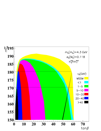
Figure 8: Top quark mass as a function of $\tan\beta$ for different values of the R–Parity violating parameter $v_{3}$. Bottom quark and tau lepton Yukawa couplings are unified at $M_{GUT}$. The horizontal lines correspond to the $1\sigma$ experimental $m_{t}$ determination. Points with $t-b-\tau$ unification lie in the diagonal band at high $\tan\beta$ values. We have taken $M_{SUSY}=m_{t}$.

The dependence of our results on $\alpha_{s}$ and $m_{b}$ is totally analogous to what happens in the MSSM. The upper bound on $\tan\beta$, which is $\tan\beta\raise 1.29167pt\hbox{$\;<$\kern-7.5pt\raise-4.73611pt\hbox{$\sim\;$}}61$ for $\alpha_{s}=0.118$, increases with $\alpha_{s}$ and becomes $\tan\beta\raise 1.29167pt\hbox{$\;<$\kern-7.5pt\raise-4.73611pt\hbox{$\sim\;$}}63$ (59) for $\alpha_{s}=0.122$ (0.114). The top mass value for which unification is achieved for any $\tan\beta$ value within the perturbative region increases with $\alpha_{s}$, as in the MSSM. As for the dependence on $m_{b}$, if we consider $m_{b}(m_{b})=4.1$ (4.5) GeV then the upper bound of this parameter is given by $\tan\beta\raise 1.29167pt\hbox{$\;<$\kern-7.5pt\raise-4.73611pt\hbox{$\sim\;$}}64$ (58). In addition, the MSSM region is narrower (wider) at high $\tan\beta$ compared with the $m_{b}(m_{b})=4.3$ GeV case. The line at high $\tan\beta$ values corresponds to points where $t-b-\tau$ unification is achieved. Since the region with $|v_{3}|<5$ GeV overlaps with the MSSM region, it follows that $t-b-\tau$ unification is possible in this model for values of $|v_{3}|$ up to about 5 GeV, instead of 50 GeV or so, which holds in the case of bottom-tau unification.

References

• [1] OPAL Collaboration, L3 Collaboration, DELPHI Collaboration, ALEPH Collaboration, LEP Electroweak Working Group, and SLD Heavy Flavor Group, preprint CERN-PPE/97-154.
• [2] S. Weinberg, Phys. Rev. Lett. 19 (1967) 1264; A. Salam, in ”Elementary Particle Theory”, ed. N. Svartholm, p. 367, Stockholm (1968); S.L. Glashow, J. Iliopoulos, and L. Maiani, Phys. Rev. D2 (1970) 1285.
• [3] CDF Collaboration, F. Abe et al., Phys. Rev. Lett. 75 (1995) 1028; D0 Collaboration, S. Abachi et al., Phys. Rev. Lett. 77 (1997) 3303; Phys. Rev. Lett. 78 (1997) 3634.
• [4] ALEPH Collaboration, R. Barate et al., Phys. Lett. B422 (1998)) 369; DELPHI Collaboration, P. Abreu it al., Phys. Lett. B397 (1997) 158; Phys. Lett. B423 (1998) 194; L3 Collaboration, M. Acciari et al. Phys. Lett. B403 (1997) 168; Phys. Lett. B413 (1997) 176; OPAL Collaboration, K. Ackerstaff et al. Phys. Lett. B397 (1997) 147; Eur. Phys. J. C2 (1998) 597.
• [5] H.P. Nilles, Phys. Rep. 110 (1984) 1; H. E. Haber and G.L. Kane, Phys. Rep. 117 (1987) 75.
• [6] H. Haber et al., , Phys. Rev. Lett. 66 (1991) 1815; R. Barbieri et al., , Phys. Lett. B258 (1991) 395; J. Ellis, G. Ridolfi and F. Zwirner, Phys. Lett. B262 (1991) 477.
• [7] V Barger, G F Giudice, T Han, Phys. Rev. D40 (1989) 2987; H Dreiner and G G Ross, Oxford preprint OUTP-91-15P.
• [8] C Aulakh, R Mohapatra, Phys. Lett. B119 (1983) 136; A Santamaria, J W F Valle, Phys. Lett. B195 (1987) 423; Phys. Rev. Lett. 60 (88) 397; Phys. Rev. D39 (1989) 1780
• [9] A Masiero, J W F Valle, Phys. Lett. B251 (1990) 273
• [10] P Nogueira, J C Romão, J W F Valle, Phys. Lett. B251 (1990) 142
• [11] M C Gonzalez-Garcia, Y Nir, Phys. Lett. B232 (90) 383; P Nogueira, J C Romão, Phys. Lett. B234 (1990) 371.
• [12] J. C. Romão, C. A. Santos, and J. W. F. Valle, Phys. Lett. B288 (1992) 311.
• [13] J. C. Romão and J. W. F. Valle, Phys. Lett. B272 (1991) 436; Nucl. Phys. B381 (1992) 87.
• [14] S. Bertolini and G. Steigman, Nucl. Phys. B387 (1990) 193; M. Kawasaki et al, Nucl. Phys. B402 (1993) 323; Nucl. Phys. B419 (1994) 105; S. Dodelson, G. Gyuk and M.S. Turner, Phys. Rev. D49 (1994) 5068.
• [15] A. D. Dolgov, S. Pastor, J.C. Romão and J. W. F. Valle, Nucl. Phys. B496 (1997) 24.
• [16] J C Romão, N Rius and J W F Valle, Nucl. Phys. B363 (1991) 369.
• [17] A Jodidio et al., , Phys. Rev. D34 (1986) 1967; MARK II Collaboration, Phys. Rev. Lett. 55 (1985) 1842; Argus Collaboration, Nucl. Phys. B246 (1990) 278.
• [18] A Lopez-Fernandez, J. Romão, F. de Campos and J. W. F. Valle, Phys. Lett. B312 (1993) 240; Proceedings of Moriond ’94. pag.81-86, edited by J. Tran Thanh Van, Éditions Frontiéres, 1994.
• [19] J. C. Romão, Proceedings da International Workshop on Elementary Particle Physics Present and Future, Valencia (Spain), pags 282-294, edited by J. W. F. Valle and A. Ferrer, World Scientific 1996.
• [20] J. C. Romão, F. de Campos, M. A. Garcia-Jareno, M. B. Magro and J. W. F. Valle, Nucl. Phys. B482 (1996) 3.
• [21] F. Campos, O. Éboli, J. Rosiek and J. Valle, Phys. Rev. D55 (1997) 1316.
• [22] J. C. Romão, A. Ioannissyan and J. W. F. Valle, Phys. Rev. D55 (1997) 427.
• [23] F. de Campos, M.A. García-Jareño, A.S. Joshipura, J. Rosiek, and J.W.F. Valle, Nucl. Phys. B451 (1995) 3; R. Hempfling, Nucl. Phys. B478 (1996) 3, and hep-ph/9702412; F. Vissani and A.Yu. Smirnov, Nucl. Phys. B460 (1996) 37; H.P. Nilles and N. Polonsky, Nucl. Phys. B484 (1997) 33; B. de Carlos, P.L. White, Phys. Rev. D55 (1997) 4222; S. Roy and B. Mukhopadhyaya, Phys. Rev. D55 (1997) 7020; A.S. Joshipura and M. Nowakowski, Phys. Rev. D51 (1995) 2421.
• [24] M. A. Díaz, J. C. Romão, and J. W. F. Valle, Nucl. Phys. B524 (1998) 23.
• [25] A. Akeroyd, Marco A. Díaz and J. W. F. Valle, Phys. Lett. B441 (1998) 224.
• [26] A. Akeroyd, Marco A. Díaz, J. Ferrandis, M. A. García-Jareño, and J. W. F. Valle, Nucl. Phys. B529 (1998) 3.
• [27] M. A. Díaz, J. C. Romão, J. Ferrandis, and J. W. F. Valle, hep-ph/9801391.