Gauge Lattice Simulation of the soft QGP Dynamics

in Ultra-Relativistic Heavy-Ion Collisions

W. Pöschl and B. Müller

Department of Physics, Duke University, Durham, NC 27708-0305, USA

Abstract

In a fully relativistic approach, a RLSM description of nuclei colliding at ultra-relativistic energies can be formulated within the framework of a classical transport theory. The valence quarks of the nucleons are described through collections of classical point-like particles moving in the continuum. They are coupled to soft gluon fields which are described through the Yang Mills equations on a gauge lattice. In a first step, we focus on the range of low-$p_{t}$ interactions. Results from numerical model simulations of pure gluonic nucleus-nucleus collisions on SU(2) gauge lattices in 3+1 dimensions are presented. They show an effect which we call the glue burst.

The state of super-dense nuclear matter called the quark gluon plasma is expected to occur in the central kinematic region of ultra-relativistic heavy-ion collisions. In view of upcoming experiments at the RHIC in Brookhaven and the LHC at CERN, it is one of the most challenging topics in the physics of ultra-relativistic heavy-ion collisions to develop a coherent description of the formation of the quark gluon plasma state. Many of the descriptions which have been developed over the past years are based on the idea of a perturbative scattering of partons within transport models. One of the problems in these descriptions concerns the initial state of the colliding nuclei. The transport equations start from probability distributions of partons in the phase space. In reality however, the states of the nuclei are described by coherent parton wave functions. The incoherent parton description becomes inadequate at exchanges of small transverse momenta. A four years ago McLerran and Venugopalan proposed [1] that the proper solution of these difficulties is the perturbative expansion not around the empty QCD vacuum but around a vacuum of the mean color fields which accompany the quarks in the colliding nuclei. This idea motivates a combination of the parton cascade model [2] with a mean field description of the color fields. Before this can be done successfully, it is important to study the non-perturbative dynamics of the color mean-fields themselves.

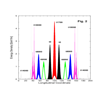
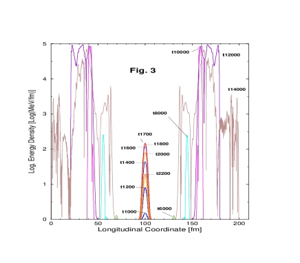
Figure 1: Transverse energy densities $w_{T}(t,x_{3})$ are displayed for selected time steps $t_{n}$

In Fig. 1, a typical scenario of a collision is displayed for times shortly before and after the collision. The figure depicts the basic idea behind our model of a combined particle-gauge lattice system. The collision describes a scenario in which two media are involved: The valence quarks, described through collections of point-like color charged particles (solid lines) and the gluon fields (helical lines). While the quarks interact essentially only through the exchange of gluons, the gluon fields are self-coupled.

     

The right-hand part of Fig. 1 displays the basic concept of our gauge lattice transport model [3]. The soft color fields are represented on a SU(2) gauge lattice in three dimensional Euclidean space and are described by the Yang-Mills equations. The quarks are represented as collections of color charged particles moving in the continuous background in position space. Their trajectories are solutions of the Wong equations. The particles are coupled with the lattice by energy and color exchange mechanisms. In SU(2) a nucleon initially is represented through a pair of quarks with opposite momenta and opposite color charge. In principle the model allows the inclusion of collision terms to describe the hard collisions between the particles. This idea has recently been submitted [3].

In recent simulations of a central collision of two nuclei with the above described model [4] it turned out that in addition to large transverse gluon radiation there exists a contribution to the transverse dynamics from “soft glue field scattering”. This leads to the question, how important is really the mean field dynamics for the transverse dynamics. Due to non-linear effects, the gluon mean field might contribute more to the transverse momenta than naively expected. We, therefore, go first one step back and focus on the pure gluon mean field dynamics in the non-perturbative regime and leave out the particles.

In short denotation the homogeneous Yang-Mills equations read ${\cal D}_{\mu}{\cal F}^{\mu\nu}=0$. An lattice version of the continuum Yang Mills equations is constructed by expressing the field amplitudes as elements of the corresponding Lie algebra, i.e. ${\cal E}_{{\vec{x}},k},{\cal B}_{{\vec{x}},k}\,\in$ LSU(2) at each lattice site $\vec{x}$. We choose the temporal gauge $A_{0}=0$ and define the following variables.

$${\cal U}_{{\vec{x}},l}=\exp(-iga_{l}{\cal A}_{l}(x))\,\,=\,\,{\cal U}^{\dagger}_{{\vec{x}}+l,-l}\qquad{\cal U}_{{\vec{x}},kl}={\cal U}_{{\vec{x}},k}\,{\cal U}_{{\vec{x}}+k,l}\,{\cal U}_{{\vec{x}}+k+l,-k}\,{\cal U}_{{\vec{x}}+l,-l}$$ (1)

In adjoint representation the color electric and color magnetic fields are expressed in terms of the above defined link variables ${\cal U}_{{\vec{x}},l}$ and plaquette variables ${\cal U}_{{\vec{x}},kl}$ in the following way.

$${\cal E}_{{\vec{x}},j}={{1}\over{iga_{j}}}\,\dot{\cal U}_{{\vec{x}},j}{\cal U}^{\dagger}_{{\vec{x}},j}\qquad{\cal B}_{{\vec{x}},j}={{i}\over{4ga_{k}a_{l}}}\,\epsilon_{jkl}\,\bigl{(}{\cal U}_{{\vec{x}},kl}-{\cal U}^{\dagger}_{{\vec{x}},kl}\bigr{)}.$$ (2)

The lattice constant in the spatial direction $l$ is denoted by $a_{l}$. We choose ${\cal U}_{{\vec{x}},i}$ and ${\cal E}_{{\vec{x}},i}$ as the basic dynamic field variables and numerically solve the following equations of motion.

$$\dot{\cal U}_{{\vec{x}},k}(t) = i\,g\,a_{k}\,{\cal E}_{{\vec{x}},k}(t)\,{\cal U}_{{\vec{x}},k}(t)\qquad\qquad\qquad\qquad\qquad$$ (3)

$$\dot{\cal E}_{{\vec{x}},k}(t) = {i\over{2ga_{1}a_{2}a_{3}}}\sum\limits^{3}_{l=1}\Bigl{\{}{\cal U}_{{\vec{x}},kl}(t)-{\cal U}^{\dagger}_{{\vec{x}},kl}(t)\,\Bigr{.}-\Bigl{.}{\cal U}^{\dagger}_{{\vec{x}}-l,l}(t)\,\Bigl{(}{\cal U}_{{\vec{x}}-l,kl}(t)-{\cal U}^{\dagger}_{{\vec{x}}-l,kl}(t)\Bigr{)}\,{\cal U}_{{\vec{x}}-l,l}(t)\,\Bigr{\}}.$$ (4)

We first study the collision of plane wave packets which have initially constant amplitude in the planes transverse to the wave vector. We choose periodic boundary conditions implying the topology of a 3-torus for our lattice. The size is chosen as 10x10x2000 lattice points. For a collision, we initially arrange two Gaussian wave packets with average momenta $(0,0,\pm\overline{k}_{z})$ and width $\Delta k_{l}$ between the maximal and minimal momenta on the lattice: $k_{l}^{min}\,\ll\,\Delta k_{l}\,\ll\,\overline{k}_{l}\,\ll\,k_{l}^{max}$ The polarization in color space is defined through the unit vectors $\vec{n}_{L}^{c}$ for the left and $\vec{n}_{R}^{c}$ for the left (L) and right (R) moving wave packet, respectively.

We express the initial conditions through the gauge fields [5]

$$A_{R/L}^{c}=\delta_{l1}{\vec{n}}^{c}_{L/R}\phi(\mp t,z-Z_{R/L})$$ (5)

where the scalar factor $\phi(t,z)$ defines the initial wave packet

$$\phi(t,x_{3}) := \phi_{0}\exp{\bigl{(}-{1\over 2}\Delta k_{3}^{2}(t+x_{3})^{2}\bigr{)}}\cos{\bigl{(}\overline{k}_{3}(t+x_{3})\bigr{)}}.$$ (6)

The amplitude factor is defined as $\phi_{0}:=\sqrt{{(2\Delta k_{3})}/({\sqrt{\pi}\sigma\overline{k}_{3}})}$ where the parameter $\sigma$ denotes the transverse area per quantum contained in the wave field. We choose the polarizations in color space $\vec{n}_{R}=\vec{n}_{L}=(0,0,1)$ for the Abelian case and $\vec{n}_{R}=(0,0,1),\,\vec{n}_{L}=(0,1,0)$ for the non-Abelian case. Once the initial fields are mapped on the lattice, the time evolution of the collision starts from the superposed initial conditions

$${\cal U}^{(0)}_{{\vec{x}},l}={\cal U}^{(0)}_{{\vec{x}},l,L}\cdot{\cal U}^{(0)}_{{\vec{x}},l,R},\qquad{\cal E}^{(0)}_{{\vec{x}},l}={\cal E}^{(0)}_{{\vec{x}},l,R}+{\cal E}^{(0)}_{{\vec{x}},l,L},$$ (7)

respectively. A linear superposition of solutions obeys the Yang-Mills equations only if these solutions have overlap zero. Therefore, the initial separation $\Delta Z$ of the wave packets may not be chosen to small.

The calculation contains four parameters. The relative isospin polarization which is parameterized through the angle $\theta_{C}$. The average momentum of the wave packets $\overline{k}$ and their width $\Delta k_{3}$ and the coupling constant g which can be rewritten in terms of the parameter $\sigma$ as $g^{\prime}=g/\sqrt{\sigma}$ by simultaneously rescaling the field ${\cal A}$ as ${\cal A}^{\prime}=\sqrt{\sigma}{\cal A}$. Consequently, the system shows the same dynamics for different values of g and $\sigma$, as long as the ratio $g^{\prime}=g/\sqrt{\sigma}$ is kept fixed.

In the following we present results from a simulated collision in the non-Abelian case with the parameters $\overline{k}_{3}=\pi/(2a_{3})$, $\Delta k_{3}=\pi/(100a_{3})$, $g=1$, $\sigma=1$. Further, we used $a_{l}=0.1\,{\rm fm}$ and $\Delta t=0.01\,{\rm fm}$. Subsequently, we refer to the direction of the collision axis (the z-axis) as the ”longitudinal direction” and to directions perpendicular to the collision axis as the ”transverse directions”. Accordingly, we define the transverse and longitudinal energy densities of the color electric field and the transverse and longitudinal energy flow distributions

$$w_{T}^{(E)}(t,z)=\sum\limits_{x,y}a_{1}a_{2}\sum\limits_{l=1}^{2}Tr\bigl{(}{\cal E}_{{\vec{x}},l}{\cal E}_{{\vec{x}},l}\bigr{)},\qquad w_{L}^{(E)}(t,z)=\sum\limits_{x,y}a_{1}a_{2}Tr\bigl{(}{\cal E}_{{\vec{x}},3}{\cal E}_{{\vec{x}},3}\bigr{)}$$ (8)

Fig. 2 displays $w_{T}^{(E)}(t_{n},z)$ plotted over the z-coordinate at various time steps $t_{n}$ as indicated on top of the curves.

         

At initial time $t_{0}$ the curves $w_{T}^{(E)}(t_{0},z)$ of the wave packets are completely filled indicating the strong oscillations according to $\overline{k}_{3}=\pi/(2a_{3})$. After 1700 time steps the wave packets are colliding and have reached maximum overlap. The smooth white zone at the bottom indicates the appearance of long wavelength modes in the Fourier spectrum of the common field. These low frequent modes have been excited in the penetration time. At time step $t_{6000}$, almost all the energy which has originally been carried by short wavelength modes around $\overline{k}_{3}$ is transmitted into long wavelength modes. This can be seen from the high frequent oscillations on the surface of the big white zones in the two receding humps. At time step $t_{8000}$ however it seems that energy is transmitted back into high frequent modes and finally the wave packets start to decay around time step $t_{10000}$. Simultaneously, we display the corresponding longitudinal energy densities $w_{L}^{(E)}(t,z)$ in Fig. 3 for the same time steps $t_{n}$ but on a logarithmic scale.

We remember that the wave packets were initially polarized into the transverse $x$-direction and consequently $w_{L}^{(E)}$ has to be zero as long as the wave packets propagate freely. However, when the two colliding wave packets of different color start overlapping, we observe an increasing longitudinal energy density in the overlap region around the center of collision at $z=100\,{\rm fm}$. Fig. 3 clearly shows that $w_{L}^{(E)}(t,z)$ grows rather fast from time step $t_{1000}$ until time step $t_{1700}$ where it reaches a maximum and has grown exponentially by more than two orders of magnitude. For larger times the hump decreases and practically disappears at $t_{3000}$. Around $t_{6000}$, however, the longitudinal energy density grows again at the positions of the receding wave packets. After 10000 time steps $w_{L}^{(E)}(z)$ has increased by five orders of magnitude. Now the question arises whether the energy deposit in longitudinal links can be associated with fields propagating into transverse directions. The transverse and longitudinal energy flow densities displayed in Fig. 4 and Fig. 5 are defined by the Poynting vector

$${\vec{\cal S}}=c\,\vec{\cal E}\times\vec{\cal B},\qquad s_{T}(t,z):=2\sum\limits_{l=1}^{2}\sum\limits_{x,y}a_{1}a_{2}\big{|}\mbox{\rm Tr}\bigr{(}\mbox{\cal S}_{l}(t,x,y,z)\bigr{)}\big{|},\qquad s_{L}(t,z):=2\sum\limits_{x,y}a_{1}a_{2}\big{|}\mbox{\rm Tr}{\cal S}_{3}(t,x,y,z)\big{|}.$$ (9)

         

A direct comparison of Fig. 4 with Fig. 3 shows that the transverse energy flow distribution $s_{T}(t,z)$ behaves very similar as compared to the longitudinal energy distributions. We call the phenomenon resulting in the strong increase of the transverse energy flow at large times the ”glue burst”. The most interesting feature is the time delay extending from time step $t_{1600}$ up to $t_{6000}$. Repeating the calculation for increasing g-values, we found that it scales with $g^{-2}$. The explanation can be found through a carefull analysis of the Yang-Mills equations. The growing peak in the center of collision clearly shows that the wave packets interact strongly due to the non-linearity of the Yang Mills equations. The wave packets, however, are restored after they have passed through each other and look for a while almost unchanged. Suddenly, around time step $t_{6000}$ they start to decay. At time step $t_{10000}$ the transverse energy flow density has grown by three orders of magnitude in comparison to the one at time step $t_{6000}$. Afterwards the energy flow density shows no further increase. A calculation for the Abelian case with same parameters shows no fragmentation of the wave packets, no transverse energy currents and no peak-like structure in the overlap region.

Fig. 5 displays the corresponding longitudinal energy current densities $s_{L}(t,z)$. As a function of time they behave similarly as the transverse energy densities $w_{T}^{(E)}(t,z)$ shown in Fig. 2. The graphs in Fig. 4 do not appear to be completely symmetrical. Matinyan et al. have shown, that the Yang Mills equations are sensitive to small perturbations. The difference in shape of the right moving and left moving energy flow distribution reveals a small difference in the initial conditions by reading them slightly asymmetrically on the lattice. This effect is enhanced in our example because we have chosen a very short initial wavelength $\overline{k}_{3}=\pi/(2a_{3})$. At high oscillations in position space, slight phase shifts can strongly change the shape of the density distribution. Nevertheless, the total integrated energies of both wave packets agree exactly. Fig. 2 to Fig. 5 are created from data obtained in one run of our computer code. A comparison of Fig. 5 with Fig. 2 shows that the asymmetry comes from the B-fields which seem to be more sensitive to perturbations. Further, a comparison of Fig. 4 with Fig. 5 shows that $s_{L}(t,z)$ in Fig. 5 decreases when $s_{T}(t,x_{3})$ in Fig. 4 increases. At time step $t_{14000}$ a sizable fraction of the longitudinal energy flow is converted into transverse energy flow. We have repeated the calculations at $\overline{k}_{3}=\pi/(100a_{3})$ and found qualitatively the same results. Here, however we demonstrate that our results are even found at the critical average longitudinal wavelength of $4a_{3}$ which is just twice as long as the shortest wavelength of $2a_{2}$ at the lattice cut-off. We also observe that the transverse energy current increases for larger $\overline{k}_{3}$.

In a study of colliding wave packets of finite extension into one transverse direction we use the same initial conditions as in the case of plane waves but multiply the function $\phi$ in Eq. (6) with a factor $\exp{\bigl{(}-(\Delta k_{y}y)^{\lambda})}$. In the simulation of the collision shown in Fig. 6 below we used the parameter values $\Delta k_{y}=1/(40a_{2})$ and $\lambda=8$ on a 4x200x800 lattice. The coupling constant was taken $g=6.0$ in order to reduce the time delay. The large value of $\lambda$ leads to a width of $8\,{\rm fm}$ in the y-direction leaving a space of $6\,{\rm fm}$ on each side of the initial wave packet. Similar results as for colliding plane waves were found. The induced transverse energy currents, however, were much larger. Fig. 6 shows the transverse energy distribution at the time steps $t100$, $t1500$, $t3500$, $t4000$, $t5000$, and $t6000$. The glue burst occurs around time step $t4000$. The full explanation of this phenomenon will be published elsewhere.

Note: The Fig. 6 exceeds the size accepted at the lanl-server and was therefore omitted. We recommend to download the postscript file from the web page http://www.phy.duke.edu/~poeschl/ under “Rsearch Related Links” and “Preprints”.

References

- [1] L. McLerran and R. Venugopalan, Phys. Rev. D49, 2233 and 3352 (1994)
- [2] K. Geiger and B. Müller, Nucl. Phys. B369, 600 (1992)
- [3] S.A. Bass, B. Müller, and W. Pöschl, Duke University preprint DUKE-TH-98-168 (nucl-th/9808011).
- [4] W. Pöschl, B. Müller, Duke University preprint DUKE-TH-98-169 (nucl-th/9808031).
- [5] C.R. Hu, et al., Phys. Rev. D 52, 2402 (1995).