Pomeron Flux Factor and Diffractive W and Jet Rates

Abstract

Experimental rates of W and dijets diffractively produced at the Tevatron Collider have recently become available. We use parametrizations of the pomeron structure function obtained from HERA data by two different schemes to compare theoretical expectations with the measured rates.

1 Introduction

The Ingelman-Schlein (IS) model [1], the first approach proposing the idea of hard diffraction, predicted that dijets could be produced in $\bar{p}p$ diffractive interactions. This kind of reaction was supposed to occur as a two-step process in which:

1) a pomeron is emitted from the quasi-elastic vertex;

2) partons of the pomeron interact with partons of the incoming proton producing jets.

One notes that the first step refers to a soft process while the second one is typically hard. In the expression proposed to calculate the dijet diffractive cross-section, the interplay between the soft and hard parts is simply conceived as a product. One assumes that factorization applies to these two steps so that

$$\frac{d^{2}\sigma_{jj}}{dtdx_{\bf I\!P}}=\frac{d^{2}\sigma_{sd}}{dtdx_{\bf I\!P}}\ \frac{\sigma_{p\bf I\!P\rightarrow jj}}{\sigma_{p\bf I\!P\rightarrow X}},$$ (1)

where $d^{2}\sigma_{sd}/{dtdx_{\bf I\!P}}$ is the cross section for single diffraction with $x_{\bf I\!P}=M^{2}_{X}/s$.

The soft term in Eq.(1), $(d^{2}\sigma_{sd}/dtdx_{\bf I\!P})(1/\sigma_{p\bf I\!P\rightarrow X}),$ has become known as the pomeron flux factor and is usually obtained from the Triple Pomeron Model [2] while $\sigma_{p\bf I\!P\rightarrow jj}$, the cross section pomeron-proton leading to dijets, is calculated from the parton model and QCD. In order to perform these calculations one has to know the pomeron structure function. This is the subject of Section 2.

The idea of hard diffractive production proposed by the IS model gave rise to a new branch of hadron physics, inspiring a lot of phenomenological studies as well as motivating projects of new experiments. On the phenomenological side, this concept was extended to processes like diffractive production of heavy flavours, $W$, $Z$, Drell-Yan pairs (see, for instance, refs.[3, 4]). In [4] appears the suggestion of the flux factor as a “distribution of pomerons in the proton”. A particular form of the standard flux is given there by

$$f(x_{\bf I\!P},t)=\frac{9b^{2}}{4\pi^{2}}[F_{1}(t)]^{2}x_{\bf I\!P}^{1-2\alpha(t)},$$ (2)

which is usually referred to as Donnachie-Landshoff flux factor.

Most of these processes were incorporated at the events generator POMPYT created by Bruni and Ingelman [5]. A more recent analysis of diffractive dijets and W production can be found in [6, 7].

As for experimental results, the UA8 Collaboration has recorded the first observations of diffractive jets [8]. This success has inspired other experimental efforts in this direction. However, subsequent analysis revealed a disagreement between data and theoretical predictions which was referred to as “discrepancy factor”.

Goulianos has suggested [9] that this discrepancy factor observed in hard diffraction has to do with the well known unitarity violation that occurs in soft diffractive dissociation and that it is caused by the flux factor given by the Triple Pomeron Model. In order to overcome this difficulty, he proposed a procedure [9] which consists of the flux factor “renormalization”, that is, the renormalized flux is defined as

$$f_{N}(x_{\bf I\!P},t)=\frac{f(x_{\bf I\!P},t)}{N(x_{\bf I\!P_{min}})},$$ (3)

where

$$N(x_{\bf I\!P_{min}})=\int_{x_{\bf I\!P_{min}}}^{x_{\bf I\!P_{max}}}dx_{\bf I\!P}\int^{t=0}_{t=-\infty}f(x_{\bf I\!P},t)dt.$$ (4)

Meanwhile, new data coming from HERA experiment has put the problem of the pomeron structure function in much more precise basis by measuring the diffractive structure function, i.e. the proton structure function tagged with rapidity gaps [10] - [12]. More recently yet, new diffractive production rates has become available from experiments performed at the Tevatron by the CDF and D0 collaborations [13] - [16].

This paper consists of a phenomenological analysis in which theoretical predictions of dijets and W diffractively produced are presented and compared to the experimental rates. These predictions take for the pomeron structure function results of an analysis performed previously [17] by using HERA data. In such an analysis both possibilities of flux factor, standard and renormalized, are considered.

2 Pomeron Structure Function from HERA

The measurements of diffractive deep inelastic scattering performed by the H1 and the ZEUS collaborations [10, 11] at HERA experiment are given in terms of the diffractive cross section

$$\frac{d^{4}\sigma_{ep\rightarrow epX}}{dxdQ^{2}dx_{\bf I\!P}dt}=\frac{4\pi\alpha^{2}}{xQ^{4}}[1-y+\frac{y^{2}}{2[1+R^{D}(x,Q^{2},x_{\bf I\!P},t)]}]F^{D(4)}_{2}(x,Q^{2},x_{\bf I\!P},t),$$ (5)

where $F^{D(4)}_{2}(x,Q^{2},x_{\bf I\!P},t)$ is the diffractive structure function (details on the notation and kinematics can be found in [17]). In these measurements $R^{D}$ was neglected and $t$ was not measured, so that the obtained data were given in terms of

$$F^{D(3)}_{2}(Q^{2},x_{\bf I\!P},\beta)=\int{F^{D(4)}_{2}(Q^{2},x_{\bf I\!P},\beta,t)\ dt}.$$ (6)

The diffractive pattern exhibited by the $F^{D(3)}_{2}$ data [10, 11] strongly suggested that the following factorization would apply,

$$F_{2}^{D(3)}=g(x_{\bf I\!P})\ F_{2}^{\bf I\!P}(\beta,Q^{2}).$$ (7)

This property is not revealed by data obtained more recently in a extended kinematical region by the H1 Collab. [12], but in such a case the violation of factorization basically takes place in the region not covered by the previous measurements and can be attributed to the existence of other contributions besides the pomeron.

Based on the IS model, one can interpret the quantities given in the above equation as $g(x_{\bf I\!P})$, the integrated-over-$t$ flux factor, and $F_{2}^{\bf I\!P}$, the pomeron structure function.

Our procedure to extract $F_{2}^{\bf I\!P}$ from HERA data is basically the following [17]:

• We assume that the factorized expression (7) (and, consequently, pomeron dominance) applies to the kinematical range covered by data given in [10, 11];

• For the integrated flux factor, that is for $g(x_{\bf I\!P})=\int f(x_{\bf I\!P},t)\ dt$, both forms, the standard (2) and the renormalized one (3), are considered;

• The pomeron structure function is given by $F_{2}^{\bf I\!P}(\beta,Q^{2})=\sum_{i}e_{i}^{2}\ \beta q(\beta,Q^{2})=2/9\ S(\beta,Q^{2})$, where $S(\beta,Q^{2})=\sum_{i=u,d,s}\ [q_{i}(\beta,Q^{2})+{\bar{q}_{i}}(\beta,Q^{2})]$ with $q_{u,{\bar{u}}}=q_{d,{\bar{d}}}=q_{s,{\bar{s}}}$;

• The quark and gluon distribution are evolved in $Q^{2}$ from a initial scale by the DGLAP equations;

• For the distributions at initial scale $Q^{2}_{0}=4$ GeV², three possibilities were considered:

1) hard-hard:

$$S(\beta,Q^{2}_{0}) = a_{1}\ \beta\ (1-\beta)$$

$$g(\beta,Q^{2}_{0}) = b_{1}\ \beta\ (1-\beta)$$

2) hard-free:

$$S(\beta,Q^{2}_{0}) = a_{1}\ \beta\ (1-\beta)$$

$$g(\beta,Q^{2}_{0}) = b_{1}\ \beta^{b_{2}}\ (1-\beta)^{b_{3}}$$

3) free-delta:

$$S(\beta,Q^{2}_{0}) = a_{1}\ \beta^{a_{2}}\ (1-\beta)^{a_{3}}$$

$$g(\beta,Q^{2}_{0}) = b_{1}\ \delta(1-\beta).$$

The detailed description of these fits and results can be found in [17]. Since for the case of renormalized flux it was difficult to establish the gluon component, a fourth possibility was used in which the initial distribution of gluons was supposed to be null. Four of these fits were selected from [17] to perform the calculation of the diffractive rates presented here. The parameters used in such calculations are shown in Table 1.

	D&L	D&L	REN	REN
	hard-hard	free-delta	hard-hard	free-zero
$a_{1}$	2.55	1.51	5.02	2.80
$a_{2}$	1	0.51	1	0.65
$a_{3}$	1	0.84	1	0.58
$b_{1}$	12.08	2.06	0.98	$-$
$b_{2}$	1	$-$	1	$-$
$b_{3}$	1	$-$	1	$-$

Table 1: Fit parameters for the pomeron structure function. The procedure used to establish these parametrizations can be found in [17].

3 Diffractive Parton Model

In this section, we present the expressions we have used to calculate the rates for diffractive production of W and jets. From the parton model, the generic expression for the cross section of these processes is

$$d\sigma_{W/jj}=f_{A}(x_{a},Q^{2})dx_{a}\ f_{B}(x_{b},Q^{2})dx_{b}\ (d{\hat{\sigma}}_{ab})_{W/jj}$$ (8)

where the parton a of the hadron A interacts with the parton b of the hadron B to give a W or a pair of partons $(c,d)$ in the case of dijets.

3.1 W production

With the elementary cross section

$${\hat{\sigma}_{ab\rightarrow W}}=\frac{2}{3}\pi{g_{W}}^{2}\ \delta(x_{a}\ x_{b}\ s-M^{2}_{W})$$ (9)

in equation (8), the integrated cross section is given by

$$\sigma(AB\rightarrow W^{\pm})=\frac{2}{3}\pi\frac{{g_{W}}^{2}}{s}\sum_{a,b}\int_{x_{a_{min}}}^{1}\frac{dx_{a}}{x_{a}}f_{A}(x_{a})\ f_{B}(x_{b}).$$ (10)

with $x_{b}={M^{2}_{W}}/{x_{a}\ s}$. For $W^{+}$ production, the interacting partons are $a=u$ and $b={\bar{d}}_{\theta_{C}}$, and for $W^{-}$ production, $a=\bar{u}$ and $b=d_{\theta_{C}}$, with $d_{\theta_{C}}=d\cos{\theta_{C}}+s\sin{\theta_{C}}$ where $\theta_{C}$ is the Cabbibo angle ($\theta_{C}\cong 13^{o}$). The kinematical limit is determined by $x_{a}\ x_{b}\ s=\hat{s}=M^{2}_{W}$, that is $x_{a_{min}}={M^{2}_{W}}/{s}$.

3.2 Dijets production

In the case of dijets generated from partons c and d, their transversal energy is

$$E_{T}=|p_{c}|\sin{\theta_{c}}=|p_{d}|\sin{\theta_{d}}.$$ (11)

By using the definition of rapidity,

$$y=\frac{1}{2}\ln{\frac{E+E_{L}}{E-E_{L}}}$$

one can get

$$e^{-y}=\frac{E_{T}}{|p_{c}|(1+\cos{\theta_{c}})}\ \ \ \ {\rm and}\ \ \ \ e^{-y^{\prime}}=\frac{E_{T}}{|p_{d}|(1+\cos{\theta_{d}})}.$$ (12)

Defining the Mandelstam variables for the parton system as

$$\hat{s}=x_{a}x_{b}s$$ (13)

and

$$\hat{t}=-2p_{a}.p_{c} = -x_{a}\ \sqrt{s}\ E_{T}\ e^{-y}=-x_{b}\ \sqrt{s}\ E_{T}\ e^{y^{\prime}},$$

one can write the Bjorken variables $x_{a}$ and $x_{b}$ as

$$x_{a}=\frac{E_{T}}{\sqrt{s}}(e^{y}\ +\ e^{y^{\prime}})\ \ \ \ {\rm and}\ \ \ \ x_{b}=\frac{E_{T}}{\sqrt{s}}(e^{-y}\ +\ e^{-y^{\prime}}).$$ (14)

Now, making use of the transformation $dx_{a}\ dx_{b}\ d\hat{t}\rightarrow 2E_{T}\ dE_{T}\ x_{a}\ x_{b}\ dy^{\prime}\ dy$ in Eq. (8), one obtains

$$\frac{d\sigma}{dy}=\sum_{a,b}\int_{E_{T_{min}}}^{E_{T_{max}}}dE_{T}^{2}\int_{y^{\prime}_{min}}^{y^{\prime}_{max}}dy^{\prime}x_{a}f_{A}(x_{a},Q^{2})x_{b}f_{B}(x_{b},Q^{2})(\frac{d\hat{\sigma}}{d\hat{t}})_{jj}.$$ (15)

In this case, the kinematical limits are

$$\ln{\frac{E_{T}}{\sqrt{s}-E_{T}\ e^{-y}}}\leq y^{\prime} \leq\ln{\frac{\sqrt{s}-E_{T}\ e^{-y}}{E_{T}}},$$

$$E_{T_{min}}=experimental\ cut \ \ \ \ {\rm and}\ \ \ \ E_{T_{max}}=\frac{\sqrt{s}}{e^{-y}+e^{y}}.$$

3.3 Diffractive Dijets and W production

In order to calculate the diffractive cross sections, we use the Pomeron structure function defined as

$$xf_{\bf I\!P}(x,Q^{2})=\int dx_{\bf I\!P}\int d\beta\ g(x_{\bf I\!P})\ \beta f_{\bf I\!P}(\beta,Q^{2})\delta(\beta-\frac{x}{x_{\bf I\!P}}).$$ (16)

Introducing this expression in Eq.(15), we obtain the cross section for diffractive dijet production,

$$\frac{d\sigma}{dy}=\sum_{a,b}\int_{E_{T_{min}}}^{E_{T_{max}}}dE_{T}^{2}\int_{y^{\prime}_{min}}^{y^{\prime}_{max}}dy^{\prime}\int_{x_{\bf I\!Pmin}}^{x_{\bf I\!Pmax}}dx_{\bf I\!P}g(x_{\bf I\!P})\ x_{a}f_{p}(x_{a},Q^{2})\ \beta f_{\bf I\!P}(\beta,Q^{2})\ (\frac{d\hat{\sigma}}{d\hat{t}})_{jj},$$ (17)

where the scale is given by $Q^{2}=E_{T}^{2}$.

As for diffractive W production, the expression obtained is

$$\sigma(p\bar{p}\rightarrow W^{\pm})=\sum_{a,b}\frac{2}{3}\pi\frac{{g_{W}}^{2}}{s}\int_{x_{\bf I\!Pmin}}^{x_{\bf I\!Pmax}}dx_{\bf I\!P}\int_{\beta_{min}}^{1}\frac{d\beta}{x_{\bf I\!P}\beta}\ g(x_{\bf I\!P})f_{\bf I\!P}(\beta,Q^{2})f_{p}(\frac{\tau}{x_{\bf I\!P}\beta},Q^{2}),$$ (18)

where $\tau=M^{2}_{W}/s$ , $\beta_{min}=\tau/x_{\bf I\!P}$ and $Q^{2}=M^{2}_{W}$.

In all of these calculations, the parametrizations used for the proton structure function were taken from ref.[18].

4 Results and discussion

The experimental rate for diffractive production of W is [13] $R_{W}\ =\ (1.15\pm 0.55)\ \%$. Table 2 summarizes the experimental data from [14, 15, 16] referring to the diffractive production rates of dijets as well as the kinematical cuts used to obtain these data.

CUTS	CDF (Rap-Gap)	CDF (Roman Pots)	D0 1800	D0 630
rapidity	$-3.5\leq y\leq-1.8$	$-3.5\leq y\leq-1.8$	$-4.1\leq y\leq-1.6$	$-4.1\leq y\leq-1.6$
$x_{\bf I\!P}$	$x_{\bf I\!P}\leq 0.1$	$0.05\leq x_{\bf I\!P}\leq 0.1$	$x_{\bf I\!P}\leq 0.1$	$x_{\bf I\!P}\leq 0.1$
$E_{T}(min)$	$20\ GeV$	$10\ GeV$	$12\ GeV$	$12\ GeV$
RATES	$0.75\pm 0.10$ (2j+3j)	$0.109\pm 0.016$
			$0.67\pm 0.05$	1-2
(%)	1.53* (2j)	(2j)

Table 2: Experimental data of diffractive production of dijets and kinematical cuts. In the first column, the rate includes contribution of a third jet. The number given below indicated with an asterisk is the rate corrected to dijets only.

In Figs.1-4, we present the rapidity distributions of jet cross section obtained with different parametrizations for the pomeron structure function and for both flux factors.

The experimental data are shown again in Table 3 in comparison with the rates obtained from our theoretical calculations. The results obtained with the standard (Donnachie-Landshoff) flux are indicated by D & L, while the columns indicated as REN give the results obtained with the renormalized (Goulianos) flux. By looking at these results, we can note the following:

• The rates obtained with standard flux are much larger than the experimental values, being that these discrepancies are more pronounced for hard gluon distributions;

• Generally speaking, the rates obtained with the renormalized flux are very close to the experimental data;

• The experimental rate for the case of dijets-CDF obtained with rapidity gaps increases when one excludes the contamination with the third jets (see Table 2 , second column); thus we see that the renormalized flux generally underestimates the rates except for the case of jets-CDF obtained with roman pots, in which the contrary happens;

• A lack of W’s is noticed in the renormalized case in spite of the fact that the pomeron structure function for this case implies that the quark component is pratically the double of the gluon component [17].

5 Concluding remarks

The results of W and dijet production rates presented in this paper show that, in order to make the theoretical predictions obtained with the pomeron structure function extracted from HERA data compatible with experimental data of such rates, a renormalization procedure (or something alike) is indispensable. Of course, this conclusion is conditioned by the presumptions that underlie the approach used here, that is the Ingelman-Schlein model.

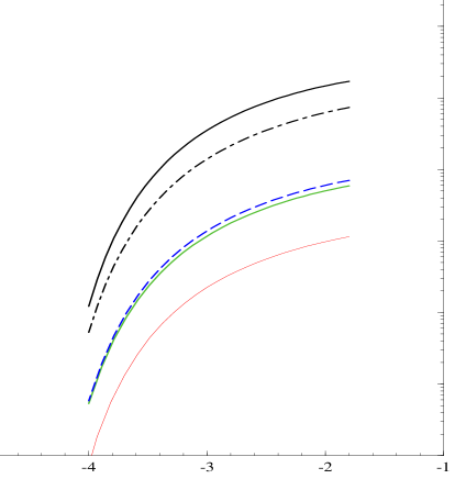
Figure 1: Rapidity distribution of dijet production. Kinematical cuts corresponding to the CDF experiment [14].

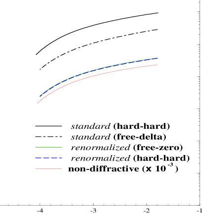
Figure 2: Rapidity distribution of dijet production. Kinematical cuts corresponding to the CDF experiment [15].

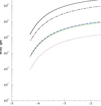
Figure 3: Rapidity distribution of dijet production for 1800 GeV. Kinematical cuts corresponding to the D0 experiment [16].

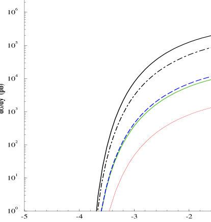
Figure 4: Rapidity distribution of dijet production for 630 GeV. Kinematical cuts corresponding to the D0 experiment [16].

References

• [1] G.Ingelman, P.E.Schlein, Phys. Lett. B 152, 256 (1985).
• [2] P. D. B. Collins, An Introduction to Regge Theory and High Energy Physics, (Cambridge University Press, Cambridge, England, 1977).
• [3] H. Fritzsch, K.-H. Streng, Phys. Lett. B 164, 391 (1985).
• [4] A. Donnachie, P.V.Landshoff, Nucl. Phys. B 303, 634 (1988).
• [5] P.Bruni, G.Ingelman, Phys. Lett. B 311, 317 (1993); preprint DESY 93-187 (1993).
• [6] L.Alvero, J.C.Collins, J. Terron, J.Whitmore, preprint PSU/TH/177 , hep-ph/9805268.
• [7] J. Whitmore, Proceedings of the Workshop on Diffractive Physics LISHEP 98, Rio de Janeiro, February 1998.
• [8] R. Bonino et al. (UA8 Collaboration), Phys. Lett. B 211, 239 (1988).
• [9] K. Goulianos, Phys. Lett. B 358, 379 (1995).
• [10] T. Ahmed et al. (H1 Collaboration), Phys. Lett. B 348, 681 (1995).
• [11] M. Derrick et al. (ZEUS Collaboration), Zeit. Phys. C 68, 569 (1995).
• [12] C. Adloff et al. (H1 Collaboration), Zeit. Phys. C 76, 613 (1997).
• [13] F. Abe et al. (CDF Collaboration), Phys.Rev.Lett. 78, 2698 (1997).
• [14] F. Abe et al. (CDF Collaboration), Phys. Rev. Lett. 79, 2636 (1997).
• [15] M. G. Albrow, Proceedings of the VII Blois Workshop (to be published).
• [16] S. Abachi et al. (D0 Collaboration), paper presented at the 28th Int. Conf. on High Energy Physics (ICHEP 96), Warsaw, Poland (July 1996).
• [17] R.J.M.Covolan, M.S.Soares, Phys. Rev. D 57, 180 (1998).
• [18] M.Gluck, E.Reya, A.Vogt, Zeit. Phys. C 67, 433 (1995).
Refer to caption