Leading particle effect, inelasticity and the connection between average multiplicities in $e^{+}e^{-}$ and $pp$ processes

Abstract

The Regge-Mueller formalism is used to describe the inclusive spectrum of the proton in $pp$ collisions. From such a description the energy dependences of both average inelasticity and leading proton multiplicity are calculated. These quantities are then used to establish the connection between the average charged particle multiplicities measured in $e^{+}e^{-}$ and $pp/{\bar{p}}p$ processes. The description obtained for the leading proton cross section implies that Feynman scaling is strongly violated only at the extreme values of $x_{F}$, that is at the central region ($x_{F}\approx 0$) and at the diffraction region ($x_{F}\approx 1$), while it is approximately observed in the intermediate region of the spectrum.

1 Introduction

It is experimentally well known that the energy dependence of the charged particle multiplicities in $e^{+}e^{-}$ and $pp/{\bar{p}}p$ processes exhibit a quite similar behavior. In the late 70’s, experiments analysing $pp$ collisions at the CERN ISR Collider [1] have shown that not the total center-of-mass energy $\sqrt{s}$ is used for particle production; instead, a considerable fraction of the available energy is carried away by the leading proton. These experiments have shown that a more adequate way of comparing average multiplicities from different reactions is in terms of the amount of energy effectively used for multiparticle production. The problem is how to determine this quantity.

Observations like these have inspired several attempts to describe ${\langle n_{ch}\rangle}_{e^{+}e^{-}}$ and ${\langle n_{ch}\rangle}_{pp}$ by an universal function. In ref.[2], for instance, two corrections are made to compare these quantities: the energy variable for ${\langle n_{ch}\rangle}_{pp}$ is corrected by removing the portion referring to the elasticity (the fraction of the energy taken by the leading particle) and then the average leading proton multiplicity is subtracted. A similar idea is followed in ref.[3] where attempts are made to establish this universal behavior by fitting.

In the present paper, we analyze the same subject by following an analagous point of view, but rephrasing the procedure in the following way. It is assumed that, if in $e^{+}e^{-}$ collisions the average charged particle multiplicity is given by

$${\langle n_{ch}\rangle}_{e^{+}e^{-}}=N(\sqrt{s}),$$ (1)

then in ${pp}/{\bar{p}}p$ collisons we have

$${\langle n_{ch}\rangle}_{pp}=\langle n_{0}\rangle+N(\langle k_{p}\rangle\sqrt{s}),$$ (2)

where $N(W)$ is an universal function of the energy available for multiparticle production, $W$, $\langle n_{0}\rangle$ is the average leading particle multiplicity, and $\langle k_{p}\rangle$ is the average inelasticity. In [2] and [3], the quantities related to $\langle n_{0}\rangle$ and $\langle k_{p}\rangle$ are supposed to be constant. In particular, in [3] they are determined by a simultaneous fit of ${\langle n_{ch}\rangle}_{e^{+}e^{-}}$ and ${\langle n_{ch}\rangle}_{pp}$ data.

Our procedure, instead, consists in obtainning these quantities ($\langle n_{0}\rangle$ and $\langle k_{p}\rangle$) not from fitting ${\langle n_{ch}\rangle}_{e^{+}e^{-}}$ and ${\langle n_{ch}\rangle}_{pp}$, but in a totally independent way, from the inclusive reaction $pp\rightarrow pX$, paying particular attention to their energy dependence. After doing that, the obtained $\langle n_{0}\rangle$ and $\langle k_{p}\rangle$ are applied to (2) via a parametrization of (1) and the result is compared to data in order to verify to what extent such a hypothesis is acceptable.

This procedure seems to be very well defined and straightforward, but it should be noticed that it drives to some difficult problems. The question is that it requires a previous knowledge about the energy dependence of the inelasticity and about the behavior of the average leading particle multiplicity which constitute themselves problematic subjects. In particular, the energy dependence of the average inelasticity is a very much disputed question since there are opposite claims that this quantity increases [4, 5, 6, 7] or that it decreases [8, 9, 10] with increasing energy at quite different rates. In spite of the of models predicting extreme behaviors, i.e. very fast increase of the inelasticity (like in [6]) or very fast decrease (like in [8]), most of these analyses referred here report the average inelasticity as having a smooth and slowly changing behavior. This is once again verified here in a different way.

The idea of discussing the energy behavior of the average inelasticity in connection with the energy dependence of $\langle n_{0}\rangle$ and $\langle k_{p}\rangle$ is not new. Of particular interest to present work is an analysis with this purpose performed by He [10]. He has extracted values of the average inelasticity by using arguments similar to those given above and obtained results pretty much in agreement with the predictions of ref.[8]. We shall argue below that such an agreement is probably due to the fact that two important effects are missing in his analysis.

Another controversial question involved in the present analysis (but treated here just en passant) is that referred to unitarity violation in diffractive dissociation processes. This is an old-standing problem that has come back to the scene due to the fact that recent measurements on hard diffractive production of jets and W’s revealed a large discrepancy between data and theoretical predictions. In ref. [12], it is proposed that such a discrepancy in hard diffraction has to do with unitarity violation in single diffractive processes. Since we are going to describe the inclusive reaction $pp\rightarrow pX$, we have to face this problem in the region of the spectrum where diffractive processes are dominant.

A by-product of the present analysis is a complete parametrization for the reaction $pp\rightarrow pX$ in the whole phase space. This is obtained basically within the Regge-Mueller approach [13], but including the modifications suggested in [12] for the diffractive contribution.

The paper is organized as follows. In Section 2 we present the theoretical framework used to describe the leading particle sprectrum. Section 3 is devoted to show how this formalism is applied to describe the experimental data. In Section 4 we discuss the connection between ${\langle n_{ch}\rangle}_{e^{+}e^{-}}$ and ${\langle n_{ch}\rangle}_{pp}$. Our main conclusions are summarized in Section 5.

2 Leading particle spectrum

In order to perform our analysis, we need to calculate the quantities

$$\langle n_{0}\rangle=\frac{1}{\sigma_{inel}}\int{\frac{d\sigma}{dx_{F}}\ dx_{F}}$$ (3)

and

$$\langle k_{p}\rangle=1-\langle x_{F}\rangle=1-\frac{1}{\sigma_{incl}}\ \int{x_{F}}\ \frac{d\sigma}{dx_{F}}\ dx_{F}$$ (4)

as a function of energy. We apply the Landshoff parametrization [14] $\sigma_{inel}(s)=56\ s^{-0.56}+18.16\ s^{0.08}\ [mb]$ to represent the inelastic cross section within the energy range where multiplicity data are included, and the inclusive cross section is simply given by $\sigma_{incl}\equiv\int{\frac{d\sigma}{dx_{F}}}\ dx_{F}$. Thus, the whole analysis depend on the knowledge of the leading particle spectrum ${d\sigma}/{dx_{F}}$ and its evolution with energy. The obtainment of this spectrum is detailed in the discussion that follows.

The invariant cross section for the inclusive reaction $ab\rightarrow cX$ is given by

$$E\frac{d^{3}\sigma}{d{\bf p}^{3}}=\frac{2E}{\pi{\sqrt{s}}}\frac{d^{3}\sigma}{dx_{F}\ dp_{T}^{2}}$$ (5)

where $x_{F}=2p_{L}/{\sqrt{s}}$ is the Feynman variable for the produced particle $c$ and $E,\ p_{L},\ p_{T}$ are respectively its energy, longitudinal and tranversal momenta. Particularly in the diffractive region ($x_{F}\approx 1$) such a quantity is usually expressed in terms of

$$E\frac{d^{3}\sigma}{d{\bf p}^{3}}=\frac{s}{\pi}\frac{d^{2}\sigma}{dt\ dM^{2}}=\frac{x_{E}}{\pi x_{F}}\frac{d^{2}\sigma}{dt\ d\xi},$$ (6)

with $x_{E}=2E/{\sqrt{s}}$, $\xi=M^{2}/s=1-x_{F}$ and $-t=m_{c}^{2}\ {(1-x_{F})^{2}}/{x_{F}}+{p_{T}^{2}}/{x_{F}}$. Variable $M^{2}$ is the missing mass squared defined as $M^{2}\equiv(p_{a}+p_{b}-p_{c})^{2}$.

The procedure to calculate the invariant cross section employed here comes from the Regge-Mueller formalism which consists basically of the application of the Regge theory for hadron interactions to the Mueller’s generalized optical theorem. This theorem establishes that the inclusive reaction $ab\rightarrow cX$ is connected to the elastic three-body amplitude $A(ab{\bar{c}}\rightarrow ab{\bar{c}})$ via

$$E\frac{d^{3}\sigma}{d{\bf p}^{3}}(ab\rightarrow cX)\sim\frac{1}{s}Disc_{M^{2}}\ A(ab{\bar{c}}\rightarrow ab{\bar{c}}),$$ (7)

where the discontinuity is taken across the $M^{2}$ cut of the elastic amplitude. It is assumed that this amplitude in turn is given by the Regge pole approach. Different kinematical limits imply in specific formulations for the invariant cross section at the fragmentation and central regions. In the following, we specify the concrete expressions that these formulations assume in such regions (details can be found in [13]).

A. Fragmentation Region

In our description, the invariant cross section for the reaction $pp\rightarrow pX$ at the fragmentation region is compounded of three predominant contributions which are determined within the Triple Reggeon Model (this is the particular formulation that (7) assumes in the beam fragmentation region with the limits $M^{2}\rightarrow\infty$ and $s/M^{2}\rightarrow\infty$ [13]). These contributions, depicted in Fig.2, correspond to pomeron, pion and reggeon exchanges and are referred to as $\rm I\!P\rm I\!P\rm I\!P$, $\pi\pi\rm I\!P$, $\rm I\!R\rm I\!R\rm I\!P$, respectively.

In the diffractive region, the $\rm I\!P\rm I\!P\rm I\!P$ contribution is dominant and (we assume for the reasons given below) is given by

$$\left(\frac{d^{2}\sigma}{dtd\xi}\right)_{\rm I\!P\rm I\!P\rm I\!P}=f_{\rm I\!P,Ren}(\xi,t)\times\sigma_{\rm I\!Pp}(s\xi)$$ (8)

where $f_{\rm I\!P,Ren}(\xi,t)$ is the renormalized pomeron flux factor proposed in [12] with the parameters defined in [15], that is

$$f_{\rm I\!P,Ren}(\xi,t)=\frac{f_{\rm I\!P}(\xi,t)}{N(s)}$$ (9)

with the Donnachie-Landshoff flux factor [16]

$$f_{\rm I\!P}(\xi,t)=\frac{{\beta}_{0}^{2}}{16\pi}F_{1}^{2}(t)\ \xi^{1-2{\alpha}_{\rm I\!P}(t)}$$ (10)

and

$$N(s)=\int_{1.5/s}^{1}\int^{t=0}_{-\infty}f_{\rm I\!P}(\xi,t)\ dt\ d\xi.$$ (11)

In the above expressions, $F_{1}(t)$ is the Dirac form factor,

$$F_{1}(t)=\frac{(4m^{2}-2.79t)}{(4m^{2}-t)}\ \frac{1}{(1-\frac{t}{0.71})^{2}},$$ (12)

the pomeron trajectory is $\alpha_{\rm I\!P}(t)=1+\epsilon+\alpha^{{}^{\prime}}t$ with $\epsilon=0.104$, $\alpha^{{}^{\prime}}=0.25\ GeV^{-2}$ and $\beta_{0}=6.56\ GeV^{-1}$, determined from [17]. In Eq.(8), the pomeron-proton cross section is given by

$$\sigma_{\rm I\!Pp}(M^{2})=\beta_{0}\ g_{\rm I\!P}\ (s\xi)^{\epsilon}$$ (13)

with the triple pomeron coupling determined from data as $g_{\rm I\!P}=1.21\ GeV^{-1}$.

Since this scheme to calculate the diffractive contribution is not the usual one, some comments are in order. The usual derivation of the Triple Pomeron Model gives (10), the standard flux factor, instead of (9), the renormalized one. The problem is that the standard flux factor drives to strong unitarity violation and the renormalization procedure was conceived [12] as an ad hoc way to overcome this difficulty. Although a rigorous demonstration of the renormalized scheme is still missing, it is acceptable in the sense that it provides a good description for the experimental data at the diffractive region (see a detailed discussion in [18]).

The pion contribution ($\pi\pi\rm I\!P$) is given by [19]

$$\left(\frac{d^{2}\sigma}{dtd\xi}\right)_{\pi\pi\rm I\!P}=f_{\pi}(\xi,t)\times\sigma_{\pi p}(s\xi)$$ (14)

where

$$f_{\pi}(\xi,t)=\frac{1}{4\pi}\frac{g^{2}}{4\pi}\ \frac{|t|}{(t-\rho^{2})^{2}}\ e^{b_{\pi}(t-\rho^{2})}\xi^{1-2{\alpha}_{\pi}(t)}$$ (15)

and $\alpha_{\pi}(t)=0.9(t-\rho^{2})$ with $\rho^{2}=m_{\pi}^{2}=0.02\ GeV^{2}$. We follow [20] in fixing the coupling constant in $g^{2}/4\pi=15.0$ and putting $b_{\pi}=0$ (see also [19]). The pion-proton cross section $\sigma_{\pi p}(s\xi)=10.83\ (s\xi)^{0.104}\ +\ 27.13\ (s\xi)^{-0.32}\ [mb]$ is taken from [17].

If one considers only the diffractive and near-to-diffractive regions and low $p_{T}$ ($-t\sim 0.0-0.1\ GeV^{2}$), the contributions outlined above are enough to provide a good description of the available data (see [18]). However, when one wants to consider larger $p_{T}$ and $x_{F}<0.9$, at least a third contribution is required. That is the reason why we introduce the reggeon contribution.

The reggeon contribution ($\rm I\!R\rm I\!R\rm I\!P$) is determined by

$$\left(\frac{d^{2}\sigma}{dtd\xi}\right)_{\rm I\!R\rm I\!R\rm I\!P}=f_{\rm I\!R}(\xi,t)\times\sigma_{\rm I\!Rp}(s\xi)$$ (16)

with

$$f_{\rm I\!R}(\xi,t)=\frac{{\beta}_{0{\rm I\!R}}^{2}}{16\pi}e^{2b_{\rm I\!R}t}\ \xi^{1-2{\alpha}_{{\rm I\!R}}(t)},$$ (17)

and

$$\sigma_{\rm I\!Rp}(s\xi)={\beta}_{0{\rm I\!R}}\ g_{{\rm I\!R}}(s\xi)^{\epsilon}.$$ (18)

In this case, the trajectory is assumed to be $\alpha_{{\rm I\!R}}(t)=0.5+t$ while the constants $\beta_{{\rm I\!R}}\equiv({\beta}_{0{\rm I\!R}}^{3}\ g_{\rm I\!R})$ and $b_{{\rm I\!R}}$ remain to be determined from data.

Thus, with the expressions and parameters given above, the $\rm I\!P\rm I\!P\rm I\!P$ and $\pi\pi\rm I\!P$ contributions are completely specified; only the $\rm I\!R\rm I\!R\rm I\!P$ contribution remains to have the final parameters determined.

B. Central Region

In order to describe the leading particle spectrum in the central region, we use the Double Reggeon Model [13] that gives the invariant cross section as

$$E\frac{d^{3}\sigma}{d{\bf p}^{3}}=\sum_{i,j}\ \gamma_{ij}(m_{T}^{2})\ \left|\frac{t}{s_{0}}\right|^{\alpha_{i}(0)-1}\ \left|\frac{u}{s_{0}}\right|^{\alpha_{j}(0)-1}$$ (19)

where $m_{T}=({p_{T}^{2}+m^{2}_{p}})^{1/2}$ is the transversal mass, and $u=-m_{T}\sqrt{s}\ e^{-y}$ and $t=-m_{T}\sqrt{s}\ e^{y}$ are the Mandelstam variables given in terms of the rapidity $y=ln\frac{(E+p_{L})}{m_{T}}$. Function $\gamma_{ij}(m_{T}^{2})$ corresponds to the product of the three vertices of the diagrams depicted in Fig.3. These diagrams represent the contributions taken into account in the present analysis: $\rm I\!P\rm I\!P$, $\rm I\!P\rm I\!R+\rm I\!R\rm I\!P$, and $\rm I\!R\rm I\!R$ (pion contributions are not considered in this case because they are totally covered by the others).

We assume for the coupling function $\gamma_{ij}(m_{T}^{2})$ a simple gaussian form,

$$\gamma_{ij}(m_{T}^{2})=\Gamma_{ij}\ e^{-a_{ij}m_{T}^{2}}$$ (20)

where $\Gamma_{ij}$ is a constant that already embodies the product of the couplings belonging to the triple and quartic vertices. With these definitions, the invariant cross sections for the three contributions become

$$\left(E\frac{d^{3}\sigma}{d{\bf p}^{3}}\right)_{\rm I\!P\rm I\!P}=\Gamma_{\rm I\!P\rm I\!P}\ e^{-a_{\rm I\!P\rm I\!P}m_{T}^{2}}\ (m_{T}\ \sqrt{s})^{2\epsilon},$$ (21)

$$\left(E\frac{d^{3}\sigma}{d{\bf p}^{3}}\right)_{\rm I\!P{\rm I\!R}+{\rm I\!R}\rm I\!P}=2\ \Gamma_{\rm I\!P{\rm I\!R}}\ e^{-a_{\rm I\!P{\rm I\!R}}m_{T}^{2}}\ (m_{T}\ \sqrt{s})^{\epsilon+\alpha_{{\rm I\!R}}(0)-1}\ cosh[(1+\epsilon-\alpha_{\rm I\!R}(0))y],$$ (22)

and

$$\left(E\frac{d^{3}\sigma}{d{\bf p}^{3}}\right)_{{\rm I\!R}{\rm I\!R}}=\Gamma_{{\rm I\!R}{\rm I\!R}}\ e^{-a_{{\rm I\!R}{\rm I\!R}}m_{T}^{2}}\ (m_{T}\ \sqrt{s})^{2(\alpha_{\rm I\!R}(0)-1)}.$$ (23)

In the above expressions again $\alpha_{\rm I\!R}(0)=0.5$ and $\epsilon=0.104$ [17]. Differently from the fragmentation region where almost all parameters are already established, in this region almost all of them (expect for the intercepts just mentioned) must be fixed from data.

The expressions given above could be enriched by detailing the reggeon exchange in terms of $f$, $\rho$, $\omega$, $a_{2}$, and taking into account all crossed terms, but in fact we are pursuing here a minimal description in which only the dominant and effective contributions are considered. We shall see below that these contributions are enough to provide a good description of the available data.

3 Description of experimental data

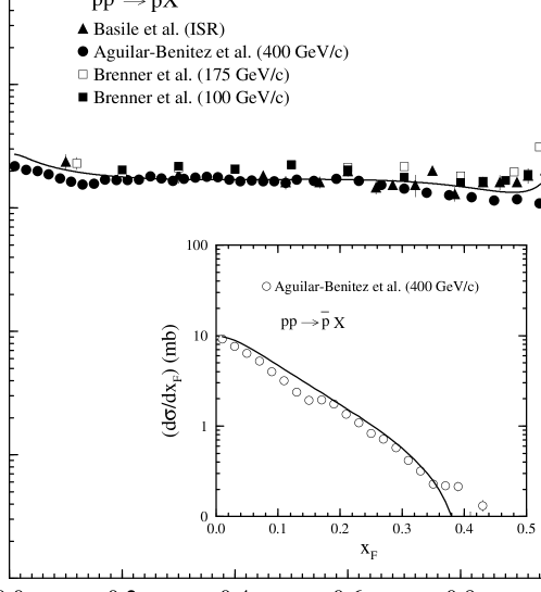
Figure 1: Inclusive spectrum for the reactions $pp\rightarrow pX$ and $pp\rightarrow{\bar{p}}X$ (in the insert). Data from [1, 21, 22]. The solid curves are the results of the fit described in the text calculated for $400\ GeV/c$.

Experimental data on leading particle spectrum are very scarce. A compilation for $pp\rightarrow pX$ is shown in Fig.1 where data from three experiments [1, 21, 22] are put together (the curve and the insert in this figure should be ignored for the moment). As can be seen, a pretty flat spectrum is exhibited, except for $x_{F}\approx 1$ where the typical diffractive peak appears.

The problem that arises when one tries to describe the $pp\rightarrow pX$ reaction in the whole phase space is that the available data are not enough to determine unambigously each one of the contributions outlined above. One may have noted in the previous section that we have summarized all secondary reggeon exchanges (except for the pion) in a single contribution denoted by $\rm I\!R$ and the reason is the following. When one analyzes, for instance, total cross section data (like in [17]), it is possible to establish (to a certain extent) the relative amount of the different contributions. Actually, this is enforced by the changing shape exhibited by the data in different regions. That is not the case here because out of the diffractive region the spectrum is pretty flat and that makes it difficult to discriminate the regions where the different exchange processes contribute the most. Thus, in order to establish how the expressions outlined above are summed up to compose the observed spectrum, we have to follow a particular strategy.

Since our intention was obtainning an acceptable description for $pp\rightarrow pX$ data in the whole phase space, we did not use in our fitting procedure the data shown in Fig.1 which represent only the $x_{F}$-dependence. Instead, we have set those data apart to be used only at the end to check our final results which, in fact, were obtained with distributions giving in terms of both $x_{F}$ and $p_{T}$ dependences.

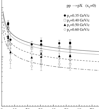
Figure 5: Invariant cross section for the reaction $pp\rightarrow pX$ at $x_{F}=0$. The description is obtained with Eq.(25). Data taken from [24].

Our procedures to determine the contributions at the central and at the fragmentation regions are quite different. The main problem is that these regions overlap each other and thus it is pratically impossible to separate them (or establish clear limits). To overcome this difficulty we assumed that, except for normalization effects, the $x_{F}$ and $p_{T}$ dependences of the proton produced in the central region through the reaction $pp\rightarrow pX$ is the same as for the antiproton produced in $pp\rightarrow{\bar{p}}X$. This assumption was implemented by fitting simultaneously the data shown in Figs. 4 and 5 [23, 24] through the expressions

$$\left(E\frac{d^{3}\sigma}{d{\bf p}^{3}}\right)_{pp->\bar{p}X}^{central}=\left(E\frac{d^{3}\sigma}{d{\bf p}^{3}}\right)_{\rm I\!P\rm I\!P}+\left(E\frac{d^{3}\sigma}{d{\bf p}^{3}}\right)_{\rm I\!P{\rm I\!R}+{\rm I\!R}\rm I\!P}+\left(E\frac{d^{3}\sigma}{d{\bf p}^{3}}\right)_{{\rm I\!R}{\rm I\!R}}$$ (24)

and

$$\left(E\frac{d^{3}\sigma}{d{\bf p}^{3}}\right)_{pp->pX}^{central}=\lambda(s)\ \left(E\frac{d^{3}\sigma}{d{\bf p}^{3}}\right)_{pp->\bar{p}X}^{central}.$$ (25)

The idea is that the data of Fig.4 provide the information on the $x_{F}$ and $p_{T}$ dependences through Eqs. (21)-(24) and relation $x_{F}=2m_{T}sinh(y)/{\sqrt{s}}$, while the connection between $pp\rightarrow{\bar{p}}X$ and $pp\rightarrow pX$ is established by fitting the data of Fig.5 through the function $\lambda(s)$ of Eq.(25). The parameters $\Gamma_{ij}$ and $a_{ij}$ of this fit are given in Table 1 while $\lambda(s)$ is parametrized as  $\lambda(s)=1.0+11.0\ s^{-0.3}$.

The agreement with data of Figs.4 and 5 is not perfect, but that is because we are simplifying the description by considering only a few contibutions, the dominant ones. As stated before, this is enough for the purposes of the present analysis.

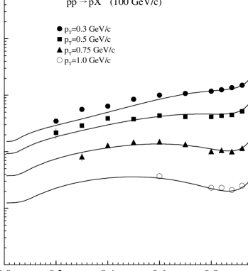
Figure 6: Invariant cross section for the $pp\rightarrow pX$ at the fragmentation region. Curves calculated with Eq.(26). Data from [22].

Now we are able to obtain the total description by adding up central and fragmentation region contributions. As explained before, the contributions dominant at the fragmentation region, Eqs. (8)-(18), are almost completely determined. The parameters $\beta_{{\rm I\!R}}$ and $b_{{\rm I\!R}}$ referring to the $\rm I\!R\rm I\!R\rm I\!P$ contribution are established by fitting the data of Fig.6 (from [22]). This is done by using the expression

$$\left(E\frac{d^{3}\sigma}{d{\bf p}^{3}}\right)_{pp->pX}^{total}=\left(E\frac{d^{3}\sigma}{d{\bf p}^{3}}\right)_{\rm I\!P\rm I\!P\rm I\!P}+\left(E\frac{d^{3}\sigma}{d{\bf p}^{3}}\right)_{\pi\pi\rm I\!P}\ +\left(E\frac{d^{3}\sigma}{d{\bf p}^{3}}\right)_{\rm I\!R\rm I\!R\rm I\!P}+\left(E\frac{d^{3}\sigma}{d{\bf p}^{3}}\right)_{pp->pX}^{central}$$ (26)

where the last term refers to Eq.(25) with the parameters given in Table 1. With this final fit the remaining parameters result to be $\beta_{{\rm I\!R}}=2465.7\ mb\ GeV^{-2}$ and $b_{\rm I\!R}=0.1\ GeV^{-2}$. Fig.7 offers a view of how the different contributions are composed to form the final result and how this picture evolves with $p_{T}$.

The different contributions of the invariant cross section in both regions integrated over $p_{T}$ produce the results of ${d\sigma}/{dx_{F}}$ for both reactions exhibited in Fig.1 (solid curves) for $p_{lab}=400\ GeV/c$. We remind the reader that these data were not used in the fit, but are used now to check the reliability of the whole procedure. From this figure it is possible to see that the final description obtained for the leading proton spectrum is quite reasonable.

4 Connection between ${\langle n_{ch}\rangle}_{e^{+}e^{-}}$ and ${\langle n_{ch}\rangle}_{pp}$

The results obtained above specify completely the behavior of the leading particle spectrum and allow us to calculate $\langle n_{0}\rangle$ and $\langle k_{p}\rangle$ as given by (3) and (4). In Fig.8, we show the energy dependence of these quantities as obtained in the present analysis (solid curves). In the same figure, it is also shown the average inelasticity as predicted by the Interacting Gluon Model (IGM) [8] (dot-dashed curve) for comparison. The average inelasticity obtained from the present analysis is very slowly increasing with energy, close to the behavior predicted by the Minijet Model [7].

With these results we can come back to our original intent which is checking the hypothesis of universal behavior of the multiplicity that is specified by Eqs.(1) and (2). In order to do that, we first establish a parametrization for $N(\sqrt{s})$ through

$$N(\sqrt{s})=a_{1}+a_{2}\ ln(\frac{s}{s_{0}})+a_{3}\ ln^{2}(\frac{s}{s_{0}})$$ (27)

with $s_{0}=1\ GeV^{2}$. However, before performing the fit to experimental data, an additional effect has to be considered. This is because, besides the charged particles produced at the primary vertex, ${\langle n_{ch}\rangle}_{e^{+}e^{-}}$ data include also decay products of $K^{0}_{s}\rightarrow\pi^{+}\pi^{-}$, $\Lambda\rightarrow p\pi^{-}$, and ${\bar{\Lambda}}\rightarrow{\bar{p}}\pi^{+}$. Following [3], we take this contamination into account by computing the ratio $R={\langle n_{ch}\rangle}_{K^{0}_{s},\Lambda,{\bar{\Lambda}}}/{{\langle n_{ch}\rangle}_{e^{+}e^{-}}}$ and by redefining (1) as

$${\langle n_{ch}\rangle}_{e^{+}e^{-}}=\frac{N(\sqrt{s})}{1-R},$$ (28)

with $R=0.097\pm 0.003$. This value was taken from [3] and, besides the references quoted therein, it is in good agreement with experimental data from ref.[25]. No energy dependence for $R$ can be inferred from these data. The fit using (27) and (28) gives $a_{1}=2.392$, $a_{2}=0.024$, and $a_{3}=0.193$.

In Fig.9, we show the above parametrization describing $\langle n_{ch}\rangle_{e^{+}e^{-}}$ data from references quoted in [26] and the calculated curve for $\langle n_{ch}\rangle_{pp}$ in comparison with data from [27]. The agreement with these data enables us to consider that our premises about the universal behavior of ${\langle n_{ch}\rangle}_{e^{+}e^{-}}$ and ${\langle n_{ch}\rangle}_{pp}$ are confirmed. Of course, this conclusion is restricted to the energy dependence of $\langle n_{0}\rangle$ and $\langle k_{p}\rangle$ shown in Fig.8.

The solid curve of the insert in Fig.9 shows what happens when the IGM average inelasticity is applied to the same purposes. One could argue that this last result is conditioned by the use of $\langle n_{0}\rangle$ obtained in the present analysis which increases with energy. However, we note that increase in $\langle n_{0}\rangle$ plays against increase in $\langle k_{p}\rangle$ since these are competitive effects.

Now a comment on the He analysis [10], where the relation

$$n_{ch}^{e^{+}e^{-}}({\sqrt{s_{e^{+}e^{-}}}})=n_{ch}^{pp}(k({\sqrt{s_{pp}}}){\sqrt{s_{pp}}})$$ (29)

is employed. After fitting $n_{ch}^{e^{+}e^{-}}$ and $n_{ch}^{pp}$ independently, He imposes that relation (29) holds and extracts the inelasticity $k$ from this assumption. This is similar to what we have done, but we think that the result of decreasing inelasticity and the agreement with IGM obtained in such an analysis comes from the fact that neither the leading particle multiplicity ($n_{0}$) nor the effect of decay products ($R$) is considered and we see no reason for ignoring such effects.

A surprising outcome of the present analysis is shown in Fig.10 (a) where the normalized cross section $1/{\sigma_{incl}}\ d\sigma/dx_{F}$ is calculated up to the LHC energy. It is shown that, if the present description holds up to such high energies, Feynman scaling is approximately observed in the intermediate fragmentation region, $0.2<x_{F}<0.8$, but is violated in opposite ways at the central and diffractive regions. Fig. 10 (b) shows the same results but in a scale that makes more evident the scaling violation at the central region. This result seems to say that the increase of production activity at the central region occurs at the expenses of a supression of the diffractive processes. However, this is just a speculative observation that should be investigated more thoroughly.

5 Conclusions

We have presented in this paper a description of the inclusive reaction $pp\rightarrow pX$ in the whole phase space within the Regge-Mueller formalism, modified by the renormalization of the diffractive cross section. The average multiplicity and the average inelasticity were obtained from the leading proton spectrum and both of them resulted to be increasing functions of energy, in agreement with [4, 5] and particularly with [7]. The energy dependence of these quantities is such that allows one to accommodate very well the charged particle multiplicities ${\langle n_{ch}\rangle}_{e^{+}e^{-}}$ and ${\langle n_{ch}\rangle}_{pp}$ by an universal function once an appropriate relation is used.

An additional result is that the normalized leading proton spectrum approximately observe Feynman scaling for intermediate $x_{F}$, whereas such scaling is violated at the central and diffractive regions.

$ij$	$\Gamma_{ij}\ (mb\ GeV^{-2})$	$a_{ij}\ (GeV^{-2})$
$\rm I\!P\rm I\!P$	$23.53$	$3.90$
$\rm I\!P{\rm I\!R}$	$-29.8$	$3.45$
${\rm I\!R}{\rm I\!R}$	$13.75$	$1.80$

Table 1: Values of the parameters $\Gamma_{ij}$ and $a_{ij}$.

Figure 2: Triple-reggeon diagrams considered in the present analysis for the reaction $pp\rightarrow pX$. The particles corresponding to the external lines are all as in the first diagram. These diagrams represent the contributions that are dominant in the fragmentation region.

Figure 3: Double-reggeon diagrams considered in the present analysis for the reaction $pp\rightarrow pX$. The particles corresponding to the external lines are all as in the first diagram. These diagrams represent the contributions that are dominant in the central region.

Figure 4: Invariant cross section for the reaction $pp\rightarrow\bar{p}X$ at the ISR energies. The description is obtained with Eqs.(21)-(24) and parameters of Table 1. Data taken from [23].

Figure 7: Invariant cross section and its contributions for $pp\rightarrow pX$ at $\sqrt{s}=53\ GeV$ for two $p_{T}$ values. These plots show how the interplay among the different contributions changes as $p_{T}$ increases.

Figure 8: Energy dependence of (a) average leading proton multiplicity $\langle n_{0}\rangle$ and (b) average inelasticity $\langle k_{p}\rangle$. In the lower figure (b) it is shown $\langle k_{p}\rangle$ obtained in the present analysis (solid curve) compared to the same quantity as predicted by the IGM [8] (dot-dashed curve).

Figure 9: Main figure: average charged particle multiplicities ${\langle n_{ch}\rangle}_{e^{+}e^{-}}$ and ${\langle n_{ch}\rangle}_{pp}$ as a function of the center-of-mass energy. The dot-dashed curve refers to the fit obtained with Eqs.(27) and (28). The solid curve was calculated with Eq.(2) by using $\langle n_{0}\rangle$ and $\langle k_{p}\rangle$ as calculated in the present analysis. Insert: the same as in the main figure, but using the average inelasticity given by the IGM [8].

Figure 10: (a) Normalized leading proton spectrum calculated up to the LHC energy. (b) The same as (a) but with logarithmic scale for $x_{F}$.

References

- [1] M. Basile et al., Phys. Lett. B 95 (1980) 31; N. Cim. 65 A (1981) 400.
- [2] M. Bardadin-Otwinoska, M. Szcekowski and A. K. Wroblewski, Z. Phys. C 13 (1982) 83.
- [3] P. V. Chliapnikov and V. A. Uvarov, Phys. Lett. B 251 (1990) 192.
- [4] J. Bellandi et al., Phys. Lett. B 262 (1991) 102; ibidem 279 (1992) 149; J. Phys. G: Nucl. Part. Phys. 18 (1992) 579; Phys. Rev. D 50 (1994) 6836.
- [5] F. O. Durães, F.S. Navarra and G. Wilk, Phys. Rev. D 47, 3049 (1993); S. Barshay and Y. Chiba, Phys. Lett. B 167 (1986) 449; J. Dias de Deus, Phys. Rev. D 32 (1985) 2334; A. B. Kaidalov and K. A. Ter-Martyrosian, Phys. Lett. B 117 (1982) 247.
- [6] B. Z. Kopeliovich et al., Phys. Rev. D 39 (1989) 769.
- [7] T. K. Gaisser et al., Proc. 21st Int. Cosmic Ray Conf. (Adelaide, 1990) vol. 8, p. 55 (ed. R. J. Protheroe); T. K. Gaisser and T. Stanev, Phys. Lett. B 219, 375 (1989).
- [8] G. N. Fowler et al., Phys. Rev. D 40, 1219 (1989).
- [9] Y. Hama and S. Samya, Phys. Rev. Lett. 78, 3070 (1997); J. Dias de Deus and A. B. Pádua, Phys. Lett. B 315, 188 (1993); Yu. M. Shabelski et al., J. Phys. G: Nucl. Part. Phys. 18, 1281 (1992); M. T. Nazirov and P. A. Usik, J. Phys. G: Nucl. Part. Phys. 18, L7 (1992); C. E. Navia et al., Prog. Theor. Phys. 88, 53 (1992); G. N. Fowler et al., Phys. Rev. D 35 (1987) 870.
- [10] Y. D. He, J. Phys. G: Nucl. Part. Phys. 19, 1953 (1993).
- [11] J. Bellandi, J. R. Fleitas and J. Dias de Deus, N. Cim. A 111 (1998) 149.
- [12] K. Goulianos, Phys. Lett. B 358 (1995) 379.
- [13] P. D. B. Collins, An Introduction to Regge theory and high energy physics, Cambridge University Press, Cambridge (1977); P. D. B. Collins and A. D. Martin, Hadron Interactions, Adam Hilger Ltd, Bristol (1984).
- [14] P. V. Landshoff, Nucl. Phys. B 12 (Proc. Suppl.) (1990) 397.
- [15] R. J. M. Covolan and M. S. Soares, Phys. Rev. D 57 (1998) 180.
- [16] A. Donnachie and P. V. Landshoff, Nucl. Phys. B 303, 634 (1988).
- [17] R. J. M. Covolan, J. Montanha, K. Goulianos, Phys. Lett. B 389, 176 (1996).
- [18] K. Goulianos and J. Montanha, Factorization and Scaling in Hadronic Diffraction, Rockefeller University Preprint: RU 97/E-43; hep-ph/9805496.
- [19] R. D. Field and G. C. Fox, Nucl. Phys. B 80 (1974) 367
- [20] B. Robinson et al., Phys. Rev. Lett. 34 (1975) 1475.
- [21] M. Aguilar-Benitez et al., Z. Phys. C 50 (1991) 405.
- [22] A. E. Brenner et al., Phys. Rev. D 26 (1982) 1497.
- [23] P. Capiluppi et al., Nucl. Phys. B 79 (1974) 189.
- [24] A. M. Rossi and G. Vannini, Nucl. Phys. B 84 (1975) 269.
- [25] TASSO Collab., M. Althoff et al., Z. Phys. C 22, 307 (1984); ibidem 27, 27 (1984); ibidem C 45, 209 (1989); L3 Collab., M. Acciarri et al., Phys. Lett. B 328, 223 (1994).
- [26] ADONE Collab., C. Bacci et al., Phys. Lett. B 86 (1972) 234; PLUTO Coll., Berger et al., Phys. Lett. B95 (1980) 313; LENA Collab., B. Niczypomk et al., Z. Phys. C 9 (1981) 1; MARKI Collab., J.L. Siegnst et al., Phys. Rev. D 26 (1982) 969; TASSO Collab., M. Althoff et al., Z. Phys. C 22 (1984) 307; AMY Collab., H.W. Zeng et al., Phys. Rev. D 42 (1990) 737; A. De Angelis, Report at the Proceedings of the XXVI Internacional Symposium on Multiparticle Dynamics, Faro (1996).
- [27] V. Blobel et al., Nucl. Phys. B 69 (1974) 454; H. Boggild et al., Nucl. Phys. B 27 (1971) 285; V. V. Ammosov et al., Phys. Lett. B 42 (1972) 519; C. Bromberg et al., Phys. Rev. D 15 (1977) 64; W. M. Morse et al., Phys. Rev. D 15 (1977) 66; D. Brick et al., Phys. Rev. D 25 (1982) 2794; A. Firestone et al., Phys. Rev. D 10 (1974) 2080; UA5 Collab., G. J. Alner et al., Phys. Lett. B 167 (1986) 476; UA5 Collab. K. Alpgard et al., Phys. Lett. B 121 (1983) 209.